the Creative Commons Attribution 4.0 License.
the Creative Commons Attribution 4.0 License.
 | 10 Jan 2022
Demistify: a large-eddy simulation (LES) and single-column model (SCM) intercomparison of radiation fog
Wayne Angevine
Jian-Wen Bao
Thierry Bergot
Ritthik Bhattacharya
Andreas Bott
Leo Ducongé
Richard Forbes
Tobias Goecke
Evelyn Grell
Adrian Hill
Adele L. Igel
Innocent Kudzotsa
Christine Lac
Bjorn Maronga
Sami Romakkaniemi
Juerg Schmidli
Johannes Schwenkel
Gert-Jan Steeneveld
Benoît Vié
An intercomparison between 10 single-column (SCM) and 5 large-eddy simulation (LES) models is presented for a radiation fog case study inspired by the Local and Non-local Fog Experiment (LANFEX) field campaign. Seven of the SCMs represent single-column equivalents of operational numerical weather prediction (NWP) models, whilst three are research-grade SCMs designed for fog simulation, and the LESs are designed to reproduce in the best manner currently possible the underlying physical processes governing fog formation. The LES model results are of variable quality and do not provide a consistent baseline against which to compare the NWP models, particularly under high aerosol or cloud droplet number concentration (CDNC) conditions. The main SCM bias appears to be toward the overdevelopment of fog, i.e. fog which is too thick, although the inter-model variability is large. In reality there is a subtle balance between water lost to the surface and water condensed into fog, and the ability of a model to accurately simulate this process strongly determines the quality of its forecast. Some NWP SCMs do not represent fundamental components of this process (e.g. cloud droplet sedimentation) and therefore are naturally hampered in their ability to deliver accurate simulations. Finally, we show that modelled fog development is as sensitive to the shape of the cloud droplet size distribution, a rarely studied or modified part of the microphysical parameterisation, as it is to the underlying aerosol or CDNC.
- Article
(7969 KB) - Full-text XML
- BibTeX
- EndNote


Most operational numerical weather prediction (NWP) centres will list errors in fog forecasting amongst their top model problems, with the requirement for improvement considered high priority (Hewson, 2019). The key customer driving this is the aviation sector, with ≈ 40 % of all delays (≈ 50 % of weather-related delays) at busy airports (such as London Heathrow, Paris CDG, San Francisco, and New Delhi) being due to low-visibility events. In the best case, these delays are inconvenient for passengers and expensive for airline operators (Cook and Tanner, 2015; Kulkarni et al., 2019). However, in the worst case, fog can also be a significant danger and is the second most likely cause of weather-related accidents (Gultepe et al., 2019; Leung et al., 2020).
Despite this importance, there is no international community working together on improving fog modelling. The Global Atmospheric System Studies (GASS) panel facilitates projects which draw together researchers from around the globe to work on specific and targeted process studies. Utilising large-eddy simulation (LES) and single-column (SCM) versions of NWP models, previous projects (including under GABLS and GCSS) have made significant advances in the understanding, and modelling of stable boundary layers (Beare et al., 2006; Cuxart et al., 2006), turbulent clouds (van der Dussen et al., 2013; Neggers et al., 2017), and aerosol–cloud interactions (Hill et al., 2015). A new GASS project related to fog modelling therefore presents an opportunity to form a community and address the challenges together, building on the previous understanding of the multitude of processes at play in radiation fog.
A previous intercomparison of radiation fog in SCM models (Bergot et al., 2007) demonstrated that even before fog onset there were considerable differences between models, and it found the model skill to be low. The current intercomparison considers a new generation of NWP SCM models, with more complex physical parameterisations, and for the first time will compare LES models for the same radiation fog event. The key questions to be considered include the following:
-
How well can models simulate the development of radiation fog?
-
What are the key processes governing the development of radiation fog, i.e. aerosol, cloud microphysics, radiation, turbulence, dew deposition, something else?
-
Which of these processes are mostly responsible for the biases seen in current NWP models?
-
What level of complexity is required from NWP models to adequately simulate these processes?
The initial phase of work, documented in this paper, will constrain the surface properties and focus primarily on the atmospheric development of fog. This will document the current state of LES and NWP fog modelling within the community and provide guidance on opportunities for improvements applicable to many models. Further stages of the project will then consider feedbacks through the land surface, more complicated cases with non-local forcing, and the representation of fog in climate models, something which has rarely been looked at in the literature.
The first intensive observational period (IOP1) of the Local and Non-local Fog Experiment (LANFEX; Price et al., 2018) presented a relatively simple case of fog forming in a nocturnal stable boundary layer, developing over several hours into turbulent, optically thick fog. However, NWP modelling of this event (Boutle et al., 2018) showed significant errors in the structure and evolution of the fog. Therefore we base the intercomparison around a slightly idealised version of IOP1. The case is based at the Met Office observational site at Cardington, UK (52.1015∘ N, 0.4159∘ W), and occurred on the night of 24–25 November 2014. Models are initialised from the 17:00 UTC radiosonde profile and forced throughout the night by the observed surface skin temperature (measured with an infra-red radiation thermometer; Price et al., 2018). No other forcing is used to keep the case simple and allow for maximum participation amongst modelling centres. This makes the case identical to the LES case presented in Boutle et al. (2018), which showed good agreement with a 3D NWP model, and testing has shown little difference to SCM results from applying advective forcing derived from the radiosondes (not shown). Forcing with surface temperature also constrains the problem to an atmospheric one, focussing on the cloud, radiation, and turbulence interaction. In reality, patchy fog began to form around 18:00 UTC, with persistent fog and visibilities around 100 m from 20:00 UTC for 12 h before clearance. The real clearance was driven by a bank of overlying cloud cover arriving at the site, which we do not attempt to represent in the simplified case.
Because of the sensitivity to cloud and aerosol processes previously discussed in Boutle et al. (2018), we request two simulations from all participants. For models which do not represent aerosol processing, the cloud droplet number concentration (CDNC) should be prescribed (if possible) as follows:
-
c10: fixed cloud droplet number concentration of 10 cm−3
-
c50: fixed cloud droplet number concentration of 50 cm−3.
For models which do represent aerosol processing, the accumulation mode aerosol should be prescribed as follows:
-
a100: initial accumulation mode (0.15 µm diameter, σ=2) aerosol of 100 cm−3
-
a650: initial accumulation mode (0.15 µm diameter, σ=2) aerosol of 650 cm−3.
Experiments c10 and a100 will be referred to as “low” aerosol/CDNC simulations, whilst c50 and a650 will be referred to as “high” aerosol/CDNC simulations. The aerosol set-up is complicated slightly, as some of the more sophisticated aerosol processing models also require specification of the Aitken and coarse mode aerosols, which are prescribed (as in Boutle et al., 2018) as 1000 cm−3 with a mean diameter of 0.05 µm and 2 cm−3 with a mean diameter of 1 µm. Vié et al. (2022) discuss how it is only really sensible to impose these additional aerosols in models which represent prognostic supersaturation of liquid water; otherwise excessive activation of the Aitken mode aerosol into cloud droplets occurs.
Although the surface temperature is specified, many models still require some parameterisation of the surface characteristics (to estimate the turbulent fluxes into the atmosphere), which is set as a flat, homogeneous, grass surface with the following parameters:
-
momentum roughness length (z0 m): 0.1 m
-
heat roughness length (z0 h): 0.001 m
-
leaf area index: 2
-
albedo: 0.25
-
emissivity: 0.98.
This set-up is derived from the characteristics of the Cardington site (Price et al., 2018). Evapotranspiration should be unrestricted (i.e. like a sea surface) to avoid complexities associated with soil moisture and land-surface models, although in practice the observed fluxes are into the surface for most of the night, and so this simplification should be of limited importance if the models can reproduce this behaviour.
Bott et al. (1990)Bott and Trautmann (2002)Angevine et al. (2018)Cotton et al. (2003)Bašták Ďurán et al. (2021)Ahlgrimm and Forbes (2014)Tonttila et al. (2017)Baldauf et al. (2011)Maronga et al. (2020)Bush et al. (2020)Dearden et al. (2018)Lac et al. (2018)Lac et al. (2018)Firl et al. (2020)Duynkerke (1991)Table 1Modelling centres, lead participants, models, and model simulations submitted. The * denotes the SCMs that have the physics package and vertical resolution of operational NWP models.
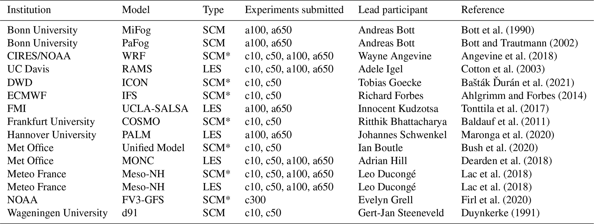
Table 2LES model details: horizontal (dx) and vertical (dz) grid length, type of aerosol processing, microphysics parameterisation details, and type of sub-grid turbulence scheme (TKE = turbulent kinetic energy closure).
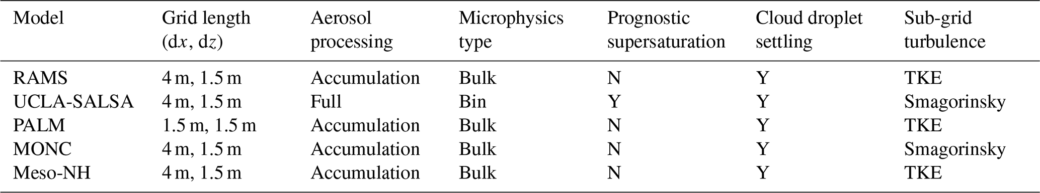
Table 3SCM model details: height of lowest model level and number of levels below 150 m, type of aerosol processing, microphysics parameterisation details, and type of sub-grid turbulence scheme (EDMF = eddy-diffusivity mass-flux closure, K1 = local first order closure, NL = non-local/counter-gradient transport, and * = modified for SCM as in Buzzi et al., 2011).
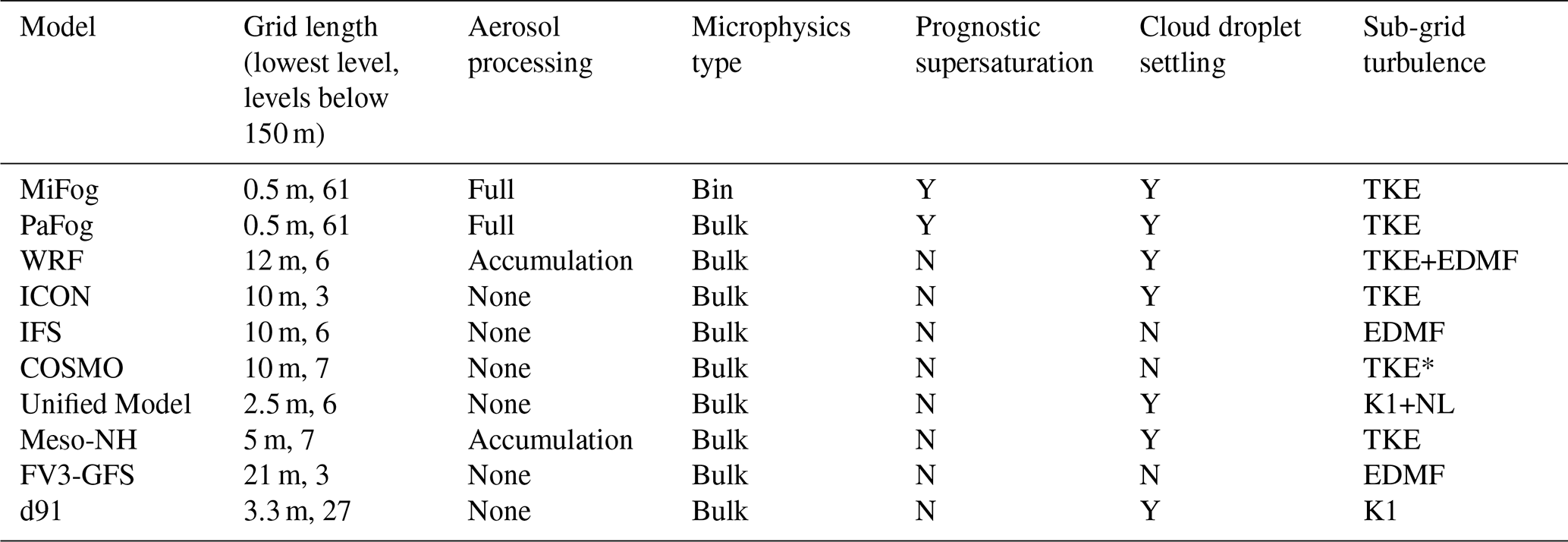
Table 1 shows the model configurations that have been submitted and are analysed in this paper, whilst Tables 2 and 3 give some further relevant details about the set-ups of the LES and SCM models respectively.
3.1 Liquid water path evolution
Figure 1 presents an initial view of the submitted models, separated by their class (LES or SCM) and aerosol or CDNC (low or high). As there is no higher-level cloud in any of the simulations, any non-zero liquid water path is attributable to fog. This is consistent with the observations until 08:00 UTC, when the upper level cloud arrived at the site and is responsible for the sharp increase in liquid water path (LWP) after this time (which should not be reproduced by the simulations). The first thing to note is that all models do at least form fog, but beyond this there is very little consistency between models.
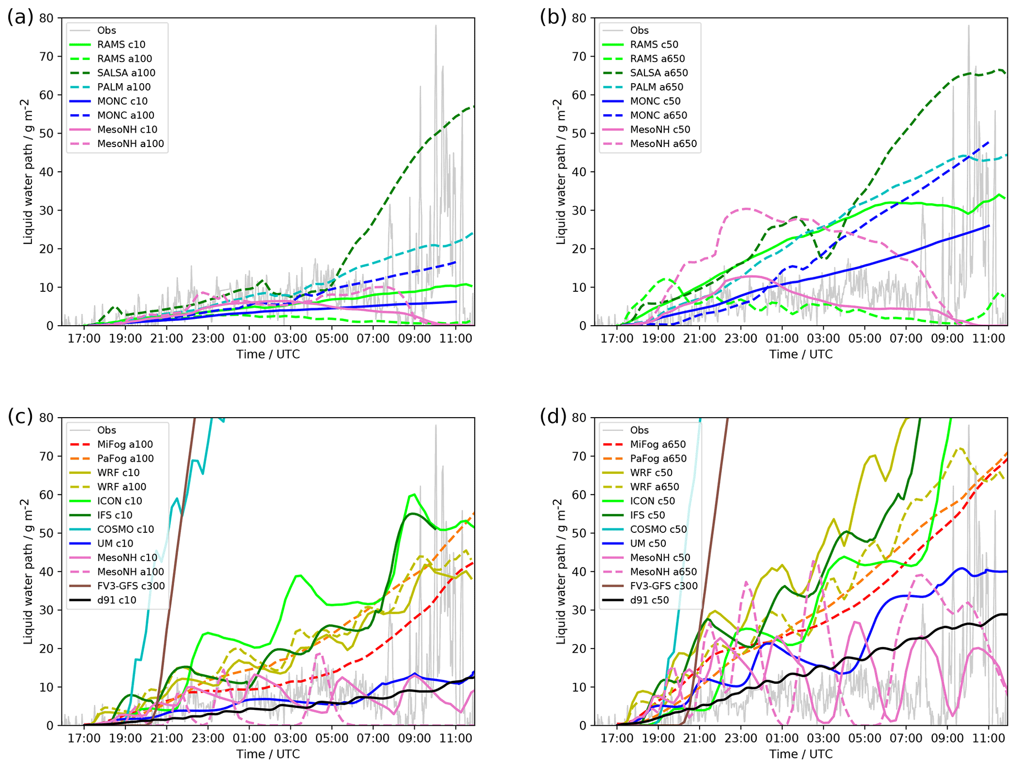
Figure 1Liquid water path observed and modelled by (a) low aerosol/CDNC LES, (b) high aerosol/CDNC LES, (c) low aerosol/CDNC SCMs, and (d) high aerosol/CDNC SCMs.
The observations are most consistent with the low aerosol/CDNC set-up. For the SCM runs, only MiFog, Meso-NH, UM, and d91 have liquid water path (LWP) evolution in line with the observations, although PaFog, IFS, and WRF are only just outside the observational range. The other models considerably overestimate the LWP. In general, the LES runs are in closer agreement with each other and the observations, but considerable spread exists between them for the high aerosol/CDNC runs. With the exception of ICON and FV3-GFS (which does not represent variable CDNC), all models show substantial variation between the low and high aerosol/CDNC set-ups, producing higher LWP with greater aerosol/CDNC.
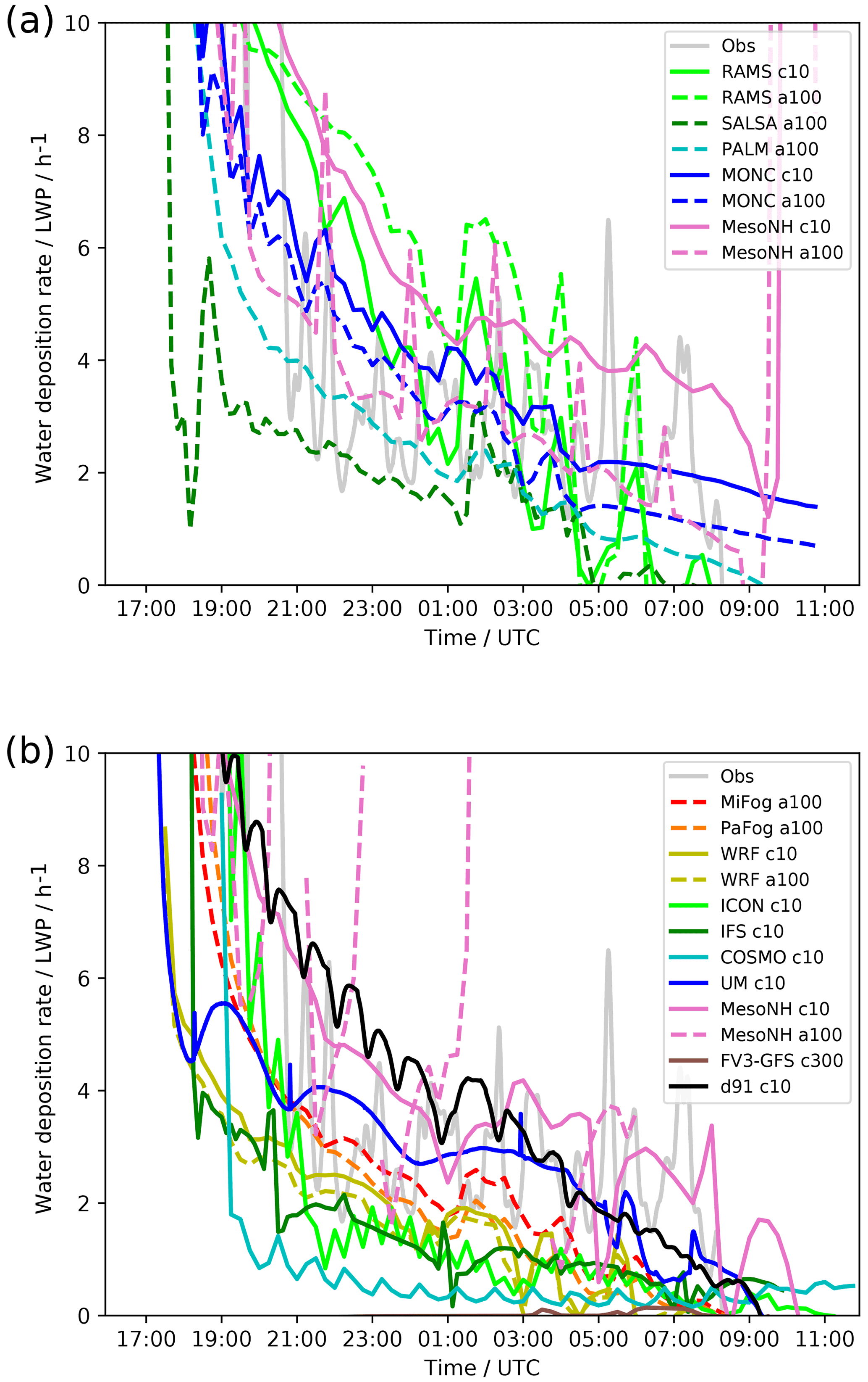
Figure 2Water deposition rate divided by liquid water path observed and modelled by (a) low aerosol/CDNC LES and (b) low aerosol/CDNC SCMs.
To leading order, the dominant factor in determining the LWP evolution of all models is the rate at which water is deposited from the atmosphere to the surface. The observations (see Boutle et al., 2018, Fig. 4a) are broadly constant at around 20 g m−2 h−1 throughout the night, and most models achieve this value despite the wildly varying LWP (possibly because the water deposition is constrained by the long-wave cooling of the atmosphere). Because the water deposition rate is strongly affected by the LWP, we must therefore normalise it before comparing the models, which is shown in Fig. 2. This shows a clear link between the deposition rate and LWP – models which do not deposit enough water onto the surface end up with LWP values which are too high, and models which deposit too much water onto the surface end up with LWP values which are too low.
The reasons for the varying water deposition rate are very model dependent, although we can try to summarise some consistent themes in the SCMs:
-
Models which do not represent cloud droplet sedimentation. These models (FV3-GFS, COSMO, IFS) are significantly hampered by their lack of this process, which is likely to be the dominant mechanism of water removal in reality. IFS is able to compensate to a certain extent by autoconverting significant amounts of fog into precipitation and removing it that way, which explains its lower LWP than COSMO or FV3-GFS, which are unable to do this. Improvements here should be easy to achieve via modifications to the microphysical parameterisation.
-
Models which produce excessive positive surface latent heat flux (Fig. 5). These models (WRF, COSMO) will always struggle to deposit enough water through microphysical processes because it is being constantly replenished via evaporation from the surface. Understanding the mechanisms behind this error can be tricky, as it may not simply be an issue with the turbulent exchange parameterisations but could also be a feedback. For example, as discussed in Boutle et al. (2018), forming fog which is slightly too optically thick can drive an erroneous positive flux, which in turn leads to further development of thicker fog.
-
The precise nature of the microphysical parameterisations responsible for water deposition. Even models which represent all processes and maintain a low latent heat flux (ICON, UM, Meso-NH) can have large discrepancies because of how the different water deposition rates feed back onto model evolution. This suggests that more work is required on the basic observations, understanding and modelling of water deposition. For example Meso-NH is the only model to represent turbulent deposition of droplets in addition to sedimentation, giving it one of the highest deposition rates.
The LES models may be closer in their behaviour but still show some similar traits to the SCMs. In particular, the models with the highest deposition rates tend to have the lowest LWP, and visa-versa. However, the mechanism by which this is achieved can be considerably different between the models. RAMS-c10 for example has a significant positive latent heat flux which is balanced by a larger cloud droplet sedimentation rate than any other LES to give an overall water deposition rate and LWP comparable to the other models. Differences like this show why it is difficult to use the LES as process models because although they are producing more consistent behaviour, the processes by which they achieve it are not consistent.
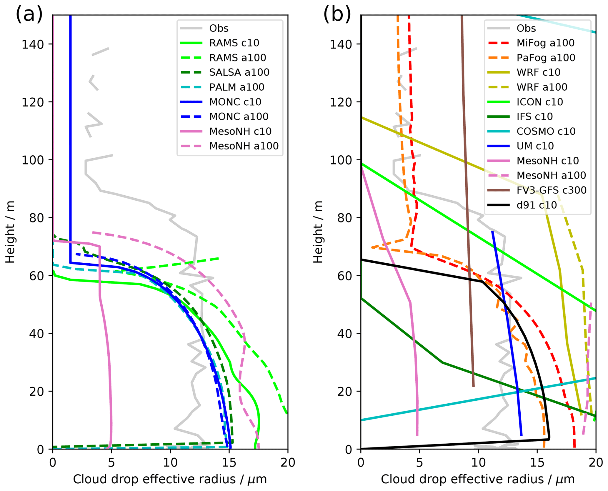
Figure 3Effective radius observed and simulated by the low aerosol/CDNC (a) LES and (b) SCMs at 00:00 UTC.
The one LES (and indeed SCM) model which does not appear to follow the pattern is Meso-NH-c10, which has one of the highest water deposition rates of any of the models, yet manages to achieve a reasonable fog simulation in all cases. This arises because it simulates a very low effective radius (Fig. 3), resulting in very strong absorption and emission from the fog layer, helping the fog to grow despite the high water deposition. The reason for the low effective radius appears to be the use of the Martin et al. (1994) parameterisation with a default “land” set-up; i.e. it is using a high (300 cm−3) assumed CDNC value in the effective radius parameterisation, rather than the actual CDNC used by the microphysical parameterisation. The Meso-NH-a100 simulation, which has a consistent link between cloud droplet number and effective radius, shows a response more consistent with the other models. This highlights the importance of using consistent assumptions between radiation and microphysical parameterisations.
The RAMS-a100 simulation has almost the opposite effect, with a high effective radius resulting in a very low LWP. This however arises because the model rapidly depletes all of the aerosol in the atmosphere and therefore has nothing to activate into cloud droplets. As a consequence, after the initial fog formation, no new small droplets are formed, but the droplets which do exist grow in size and sediment out, resulting in a very low liquid water path. This is particularly noticeable in the RAMS-a650 simulation, which has the lowest LWP of any model in the “high” experiment. Figure 4b shows that this is linked to a very low CDNC, despite the high initial aerosol concentration, because most of the aerosol has been depleted. Figure 4b also shows an interesting clustering between the full aerosol processing models, which predict CDNC values in the range 40–60 cm−3, and the accumulation only models which predict CDNC values in the range 70–90 cm−3. This shows that even though the latter group are only considering a subset of the full aerosol distribution, they may still be overestimating the activation occurring in the fog layer. However, Fig. 1b and d show that this clustering in the CDNC value does not equate to a clustering in the LWP evolution, demonstrating that there are larger differences between the models than the predicted CDNC value.
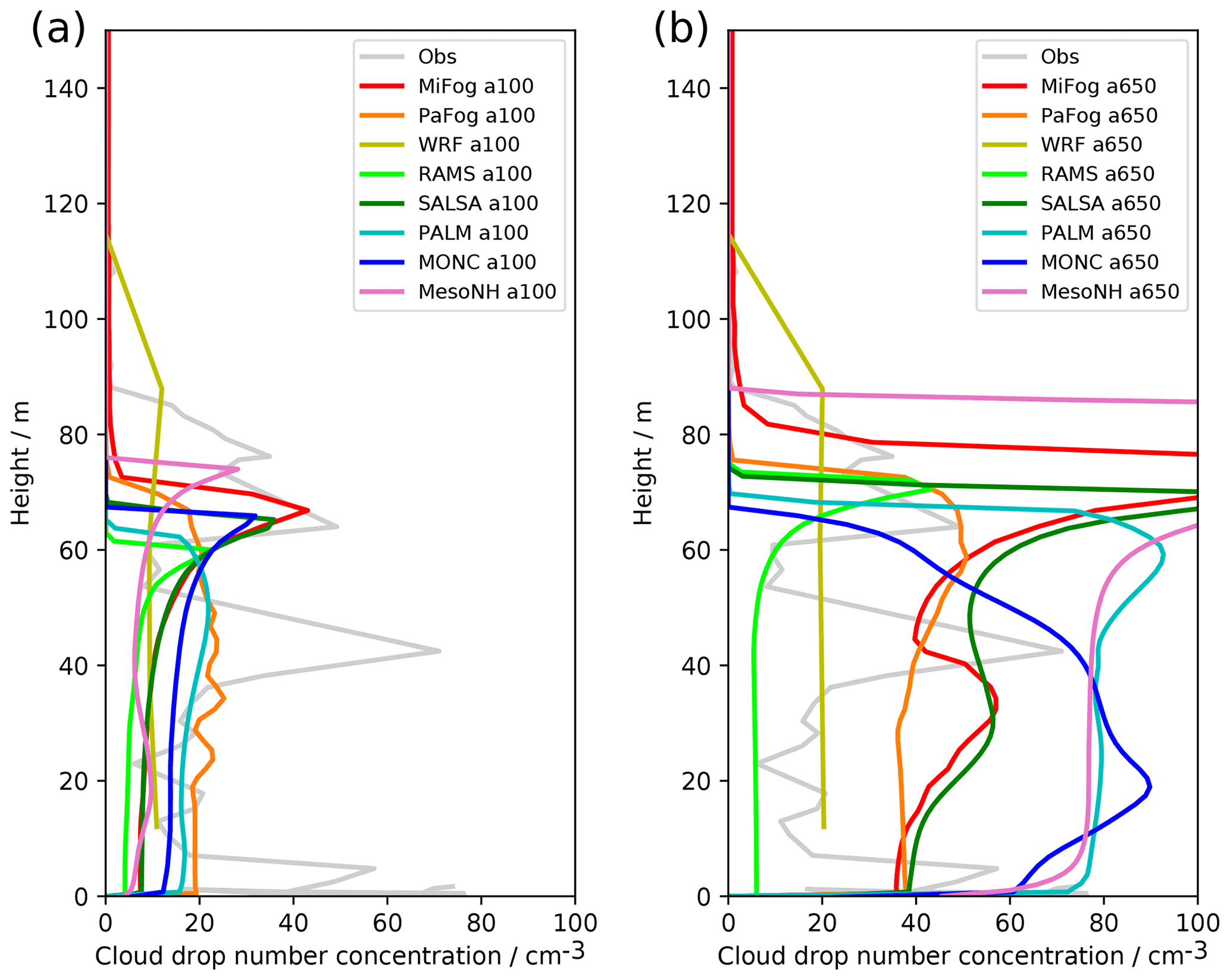
Figure 4CDNC observed and from the aerosol processing models at 00:00 UTC for (a) low aerosol and (b) high aerosol.
It is worth briefly discussing the oscillations in LWP seen in the SCM models. This is a known feature of fog SCM simulations and has been discussed previously by Tardif (2007). Long-wave (LW) cooling from the fog top is the key driver of the fog layer deepening. However, with the coarse vertical grid of the SCM models, the fog can only deepen in discrete units, when the top grows by a single model level. The LWP therefore erodes, by loss of moisture and heating from the surface, until such time as the fog can jump up a level, leading to a large increase in LWP as the water vapour in the level above is available for condensation. Hence the oscillations are created. All of the SCMs with coarse vertical grids show some oscillations, although the severity of them differs significantly. By far the simulation to suffer most is Meso-NH-a, which appears to have a further complicating feedback from the microphysics. When the fog top jumps up a level, the increase in LWP triggers significant precipitation formation, which quickly removes a large amount of water from the atmosphere. This microphysical feedback does not disappear when running Meso-NH-a at higher vertical resolution, whereas the oscillations in Meso-NH-c do (not shown) due to its use of different microphysical parameterisations.
3.2 Surface fluxes and boundary layer structure
A key feature of this fog event, and indeed many fog events, is the slow transition from a stable boundary layer with optically thin fog to a well-mixed boundary layer with optically thick fog. How this transition evolves is of key interest from a forecasting perspective as it will determine the depth and intensity of the fog layer and ultimately its duration into the following morning.

Figure 5Sensible (a, c) and latent (b, d) heat flux observed and modelled by (a, b) low aerosol/CDNC LES and (c, d) low aerosol/CDNC SCMs.
Interestingly, the LES models show greater variability in the surface sensible heat flux (Fig. 5a) than they did for the liquid water path. Whilst there is some hint towards the expected trend that models which are optically thickest (PALM, Meso-NH-c10) will generate a positive sensible heat flux and well-mixed fog layer first, RAMS-c10 sits as a clear outlier here generating the strongest positive sensible heat flux whilst having one of the thinnest (optically and physically) fog layers. It achieves this by forming a shallow but well-mixed layer in which the fog exists (Fig. 6a), capped by a strong inversion. RAMS does indeed have a higher downwelling LW radiation, which would promote development of a well-mixed fog layer. However, why it keeps this layer shallow and does not grow deeper like it does in Meso-NH is interesting, suggesting lower entrainment across the inversion. The result is that RAMS has the lowest fog top of all the LES models (Fig. 7a).
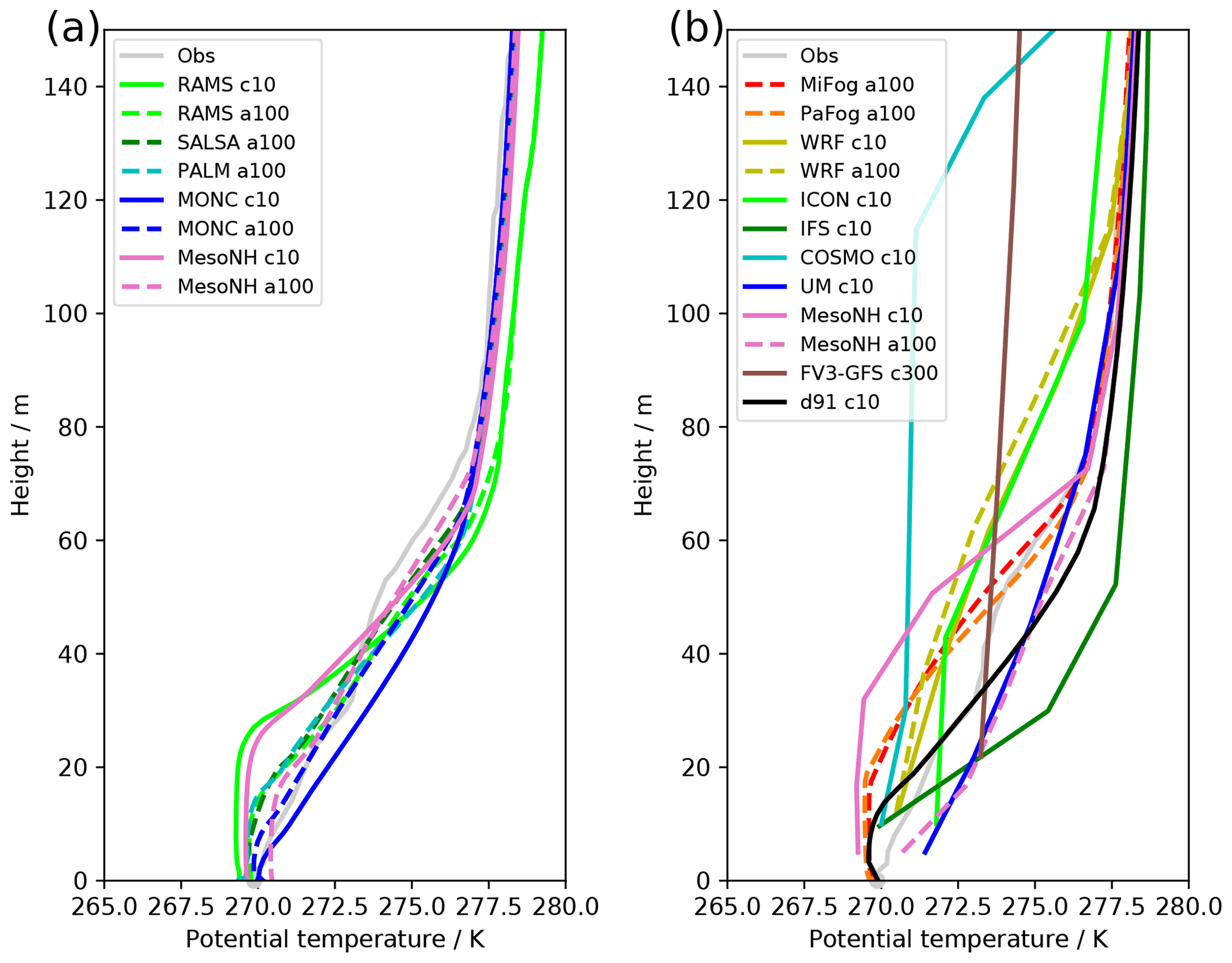
Figure 6Potential temperature observed and simulated by (a) the low aerosol/CDNC LES models and (b) the low aerosol/CDNC SCMs at 00:00 UTC.
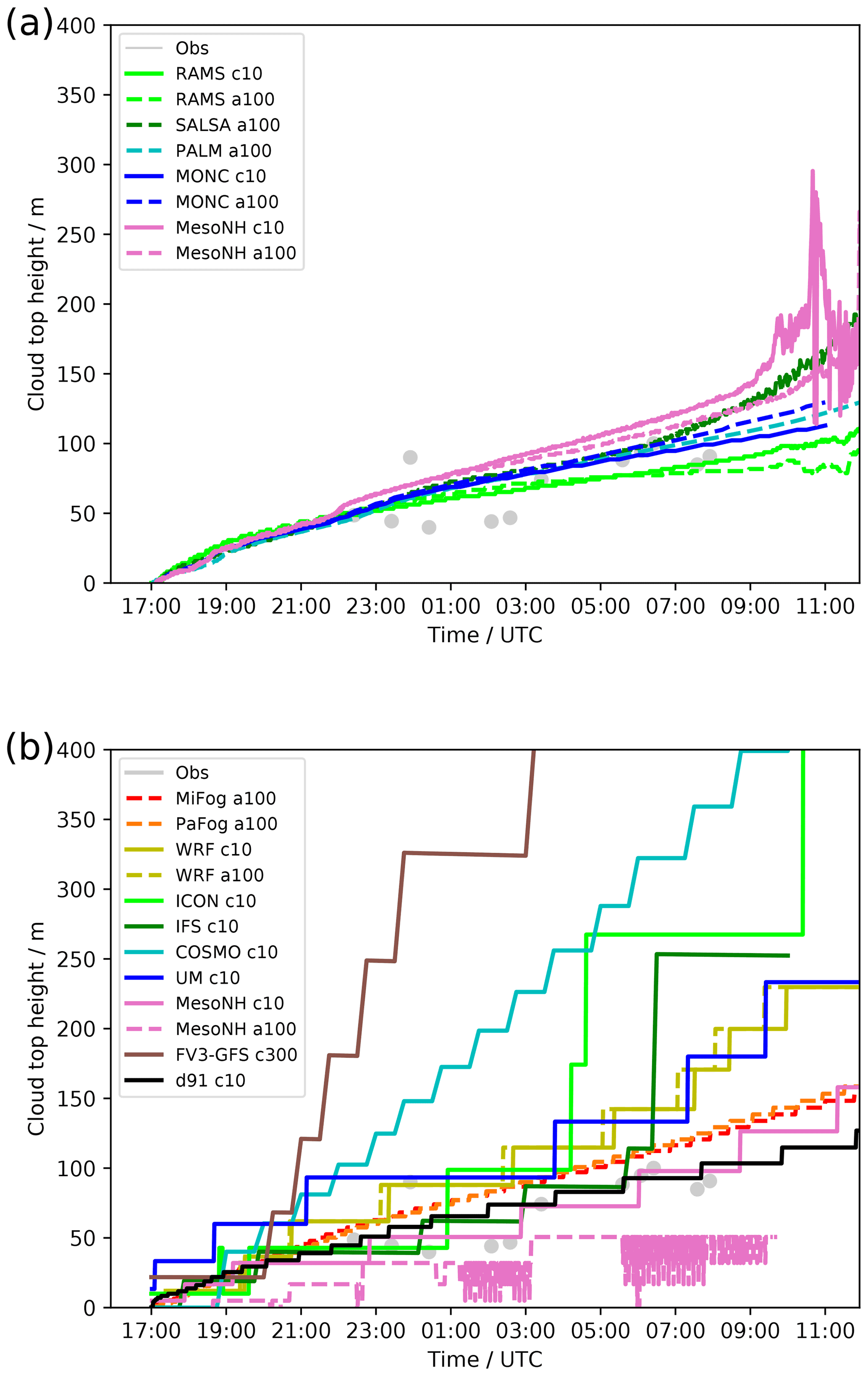
Figure 7Fog top height observed and modelled by (a) low aerosol/CDNC LES and (b) low aerosol/CDNC SCMs.
The SCMs show a similar trend to the LES models, with many producing a positive surface sensible heat flux and well-mixed boundary layer structure (Figs. 5c and 6b). However, those SCMs with close to zero sensible heat flux do maintain a stable potential temperature profile throughout the fog layer. As always, there are interesting outliers. The IFS in particular appears to manage a stable profile with a positive sensible heat flux. However, this is likely a consequence of the low vertical resolution as there are only two vertical levels within the fog layer at this stage, the first of which is well-mixed and the second is stabilised by cloud top entrainment. It is also worth discussing FV3-GFS, which is the only model which produces a negative sensible heat flux. This is possibly due to its poor vertical resolution, with the lowest model level being approximately double the height of any other model, meaning the lowest-level temperature is very warm relative to the surface. In its default set-up, FV3-GFS also produced a very negative latent heat flux, which prevented any fog formation. Therefore a lower limit of zero on the latent heat flux was imposed in their simulations to enable fog to form.
3.3 Forecasting considerations
In terms of fog impact, particularly to the aviation sector, correctly modelling fog clearance after sunrise is key to forecasting airfield clearance time and allowing full take off/landing rates to resume. There are a number of aspects of the intercomparison which complicate the simulation of the morning transition. Firstly, the unrestricted evaporation is unrealistic for a true land surface – soil moisture availability and resistance to evapotranspiration in grass will always result in less latent heat flux than our idealised set-up will produce. Secondly, the observed surface temperature warming is representative of fog which has dissipated in reality for a number of reasons not simulated by the LES and SCMs (particularly overlying cloud cover, which is responsible for the observed increase in LWP after 08:00 UTC). However, comparison between how the models deal with this situation can still provide some useful insights. As shown in Fig. 1, MesoNH-LES is the only model which completely dissipates the fog during the morning. Most models' fog evolution seems broadly unaffected by the increasing surface temperature and short-wave radiation, except for SALSA, in which it drives a large increase in LWP. There are essentially two competing mechanisms at work here. The increase in surface temperature will drive a strong positive surface moisture flux, promoting fog development. However, direct short-wave heating of the fog layer and heating due to the rise in surface temperature and positive surface heat flux will counteract this. The consequences for fog development are therefore model dependent, based on the relative importance of these processes.

Figure 8Surface downwelling short-wave radiation observed and modelled by (a) low aerosol/CDNC LES and (b) low aerosol/CDNC SCMs.
If the surface temperature was not prescribed, the key quantity driving dissipation would be the downwelling short-wave radiation (as this would drive the surface heating), which is shown in Fig. 8. The figure shows that the degree of variation between models is large (over 250 W m−2), with similar uncertainty between the LES and SCM models. To leading order, the key reason for differences in the downwelling short-wave (SW) is the LWP at sunrise – the models with the highest LWP have the lowest downwelling SW and vice versa. Optical properties of the fog appear to be much less significant here – for example comparing the UM and Meso-NH-c10 SCM simulations; Meso-NH-c10 only has a slightly smaller LWP, which offsets against its much smaller effective radius to result in almost identical downwelling SW evolution. What is clear is that there is a huge range in potential fog evolution and dissipation times driven by differences in the fog development during the night-time. Having knowledge of how realistic a model forecast of fog development through the night-time is (e.g. via real-time observations) may enable a forecaster to understand how reliable the forecast for morning dissipation is. For example, real-time equivalents of many of the observations presented here, such as radiosonde profiles, liquid water path measurement, surface heat, moisture, and radiation fluxes, would enable a much better assessment of how the fog is developing than traditional screen-level observations can provide. A comparison of these to model diagnostics will enable an assessment of whether the model is over- or under-developing fog (optically or physically) and therefore whether it is likely to dissipate earlier or later in the morning than forecast.

Figure 9Cloud base height modelled by (a) low aerosol/CDNC LES and (b) low aerosol/CDNC SCMs.
Another forecasting consideration is whether the fog will indeed dissipate or whether it will lift into low stratus. In reality, this is governed by many factors not included in this intercomparison, such as non-local advective effects or overlying cloud cover. However, some features such as fog depth and entrainment at the fog top should be captured. Figure 9 shows the cloud base height (qc>0.01 g kg−1) during the morning period for the LES and SCM models, demonstrating that there is significant variety in model simulation of this behaviour. Whilst most models keep the fog firmly on or near the ground, Meso-NH LES and COSMO SCM lift the cloud base significantly, with cloud base height exceeding 60 m (the threshold typically used by aviation for instigating low-visibility procedures) by 08:00–09:00 UTC. The difference here (and elsewhere) between Meso-NH LES and SCM is of particular interest because the physics package of both models is identical, meaning that differences must arise because of the lower vertical resolution in SCM, or because the 1D parameterised turbulence in the SCM is acting differently to the 3D resolved turbulence in the LES. In general, the dissipation results appear much more closely tied to individual models rather than characteristics of the set-up or development of the fog during the night. All models which provide both interactive and non-interactive aerosol set-ups do the same thing in both set-ups, and whilst for most this is to not break the fog, for Meso-NH it is to lift the fog. Similarly, for models which produce excessive LWP during the night, most do not break it, whilst COSMO lifts it. A more focussed intercomparison on the dissipation phase is likely required to fully understand this model-dependent behaviour and link it to physical processes.
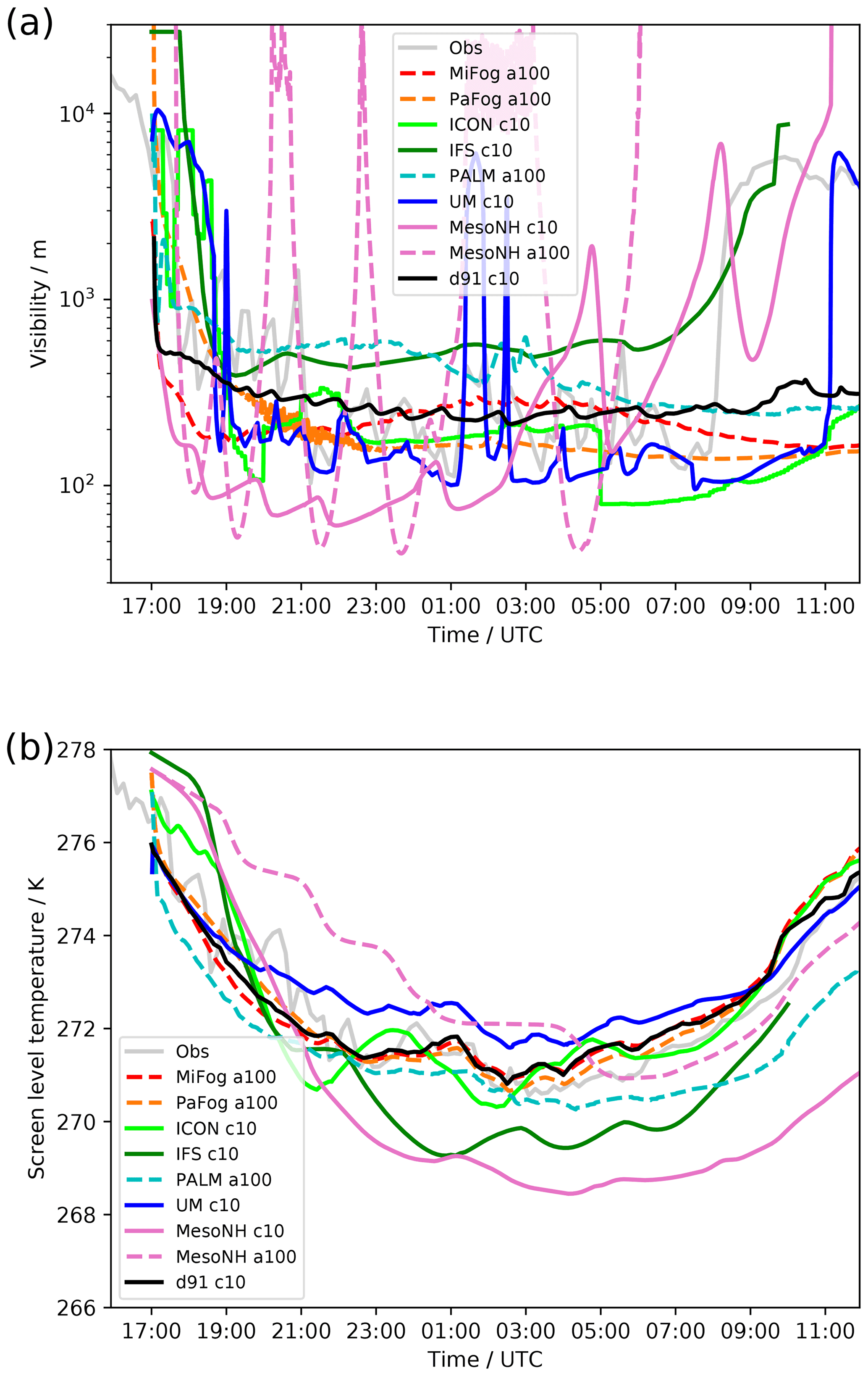
Figure 10(a) Visibility and (b) screen level temperature, observed and predicted by all models including a specific visibility parameterisation.
Finally, we discuss some of the typical metrics used by decision makers when forecasting fog events. Figure 10a shows the visibility as predicted by all models incorporating a visibility parameterisation. The visibility parameterisation is model dependent, with those used listed in Table 4. Some parameterisations utilise a direct empirical link between cloud water content and visibility, whilst others attempt to calculate the extinction coefficient directly based on the aerosol distribution and atmospheric humidity. Models for which the vertical resolution does not give a grid level at the screen-level height (1.5–3 m) either use values at the lowest model level (Table 4) or first produce input variables to the visibility parameterisation at this level via interpolation. Given the differences seen elsewhere in the fog evolution, the level of agreement between models here is somewhat surprising. Most models are forecasting visibility in the 100–300 m range for most of the night, in line with observations. IFS and PALM are forecasting slightly larger visibilities (≈ 500 m) but still below the thresholds typically used by aviation decision makers (600 m), whilst only Meso-NH produces visibilities below 100 m. Most models also retain low visibilities well into the morning period, with only Meso-NH, IFS, and eventually the UM forecasting a clearance in this metric. The consistent behaviour may, in part, be due to the tight linkage between screen-level and surface variables in many models, as with the surface temperature prescribed, the screen-level temperature does not deviate far from the observations (Fig. 10b). However, it also raises caution against the use and interpretation of such variables if they can seemingly produce such similar results despite such obvious differences in the actual simulation of fog within the models. To truly understand and interpret an NWP fog forecast requires much more than simply looking at the predicted visibility, especially in more marginal cases than this one.
Bott (2021)Bott (2021)Kunkel (1984)Gultepe et al. (2006)Gultepe et al. (2006)Clark et al. (2008)Kunkel (1984)Bott (2021)Kunkel (1984)Table 4Selected forecasting metrics for each model, as observed, and the mean and range of results for the LES and SCM models combined. Fog onset/dissipation is defined by liquid water below 60 m, whilst typical airfield low-visibility procedures (LVPs) are defined by visibility <600 m and cloud base <60 m. “>12” denotes models which did not dissipate fog by the end of the simulation.
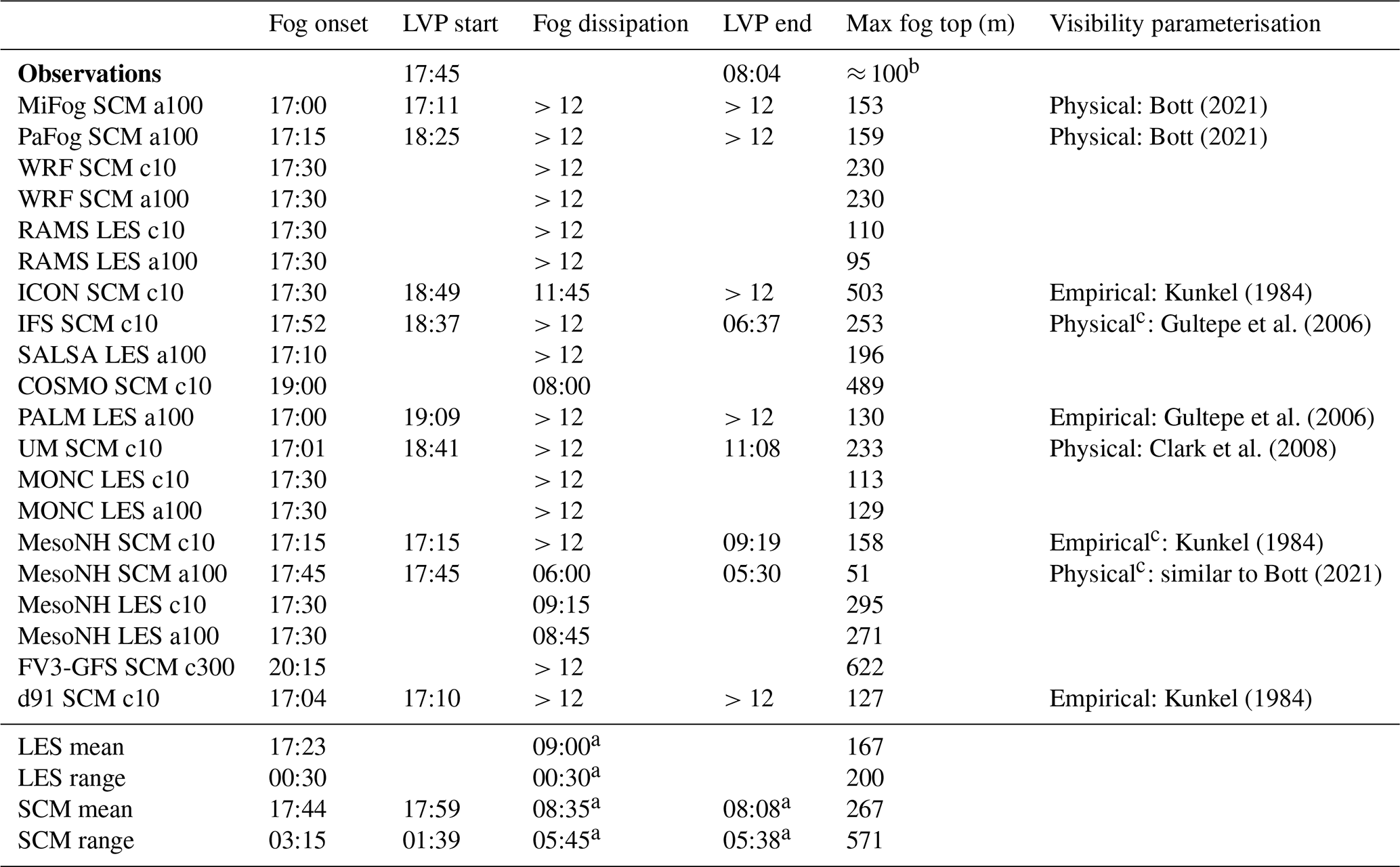
a Dissipation statistics are only calculated from the models which dissipated fog during the morning. b Recorded around 08:00 UTC just before the fog dissipated. c Parameterisations are applied at the lowest model level (Table 3) rather than the screen level.
Table 4 shows for all models the onset and dissipation time of the fog event and the maximum height reached by the fog layer. This summarises many of the themes discussed so far in the paper. The initiation of fog is handled well by all models, with the initiation happening between 17:00 and 18:00 UTC in all but two of the models. Many models show that low visibility (LVP) occurs some time after fog onset, demonstrating that the models are able to capture an initial period of thin fog where visibility remains good. The dissipation phase is much poorer, with most models persisting fog until the end of the simulation. Only a minority of models break the fog during the morning period and with no consistency in how this is done – some lifting it into stratus, whilst others clear it entirely. Whilst a few models do thin the fog sufficiently for LVP to end, it would clearly be very difficult to provide guidance to customers based on this ensemble set. The mean fog depth simulated by the SCMs is approximately 100 m higher than that from the LES and at the very top end of the LES range. This is symptomatic of the SCM behaviour in producing fog which is too thick, a characteristic that will likely lead to fog persisting for too long into the daytime.
To explore some of the themes and relationships shown in Sect. 3.1, in this section we focus on two SCMs (COSMO and UM) and one LES (MONC), modifying several parameterisations to confirm the speculated reasons for fog differences. The first and most simple test, using the UM, is to switch off cloud droplet sedimentation entirely (similar to COSMO, FV3-GFS, or IFS). This is shown in Fig. 11.
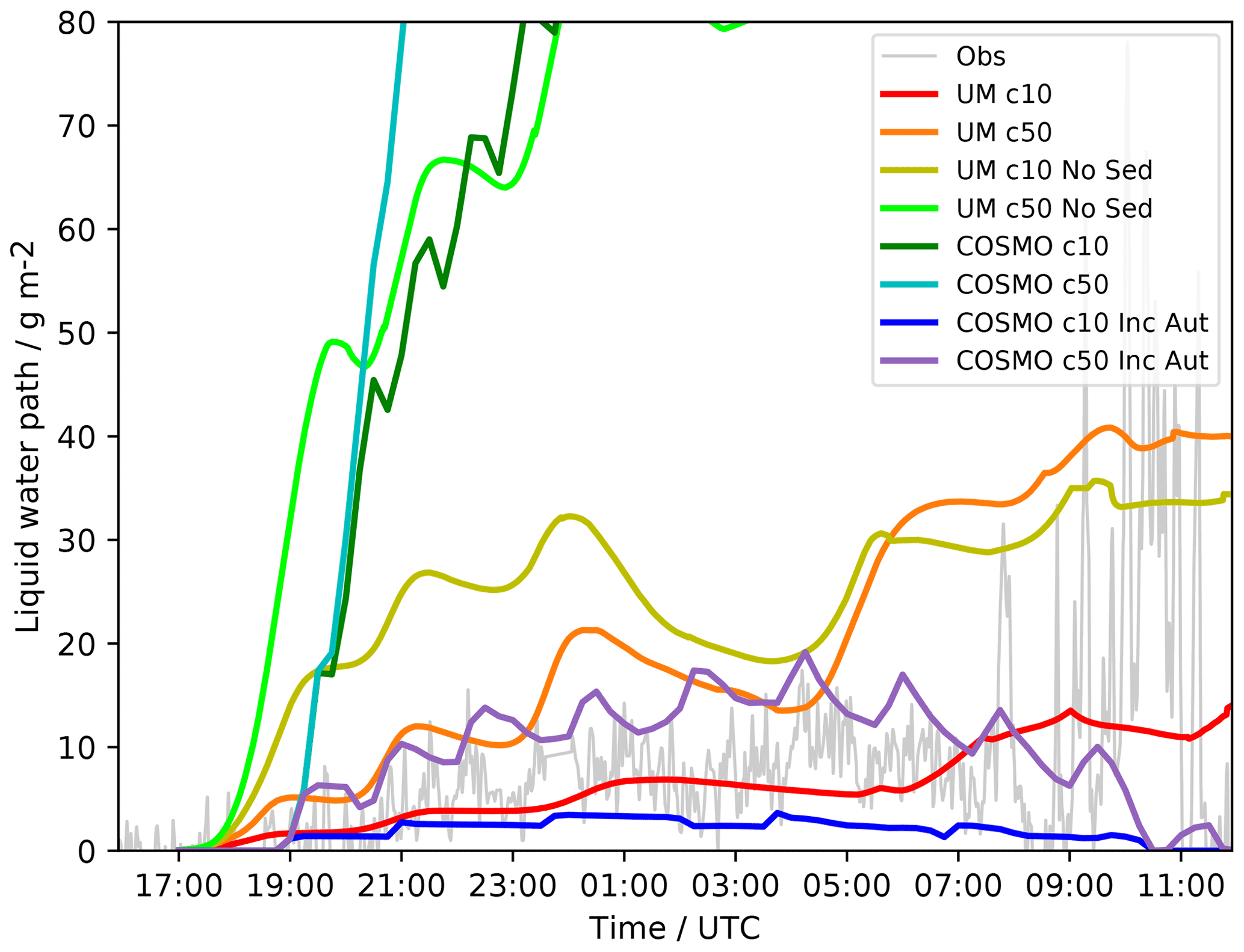
Figure 11Liquid water path observed and modelled with low and high CDNC values, from the UM with or without cloud droplet sedimentation and COSMO with low and high autoconversion rates (see caption).
The removal of cloud droplet sedimentation leads to large increases in the liquid water path for both CDNC values. Clearly the presence or absence of cloud drop sedimentation is more important than the prescription of CDNC value. This also confirms why models which do not represent this process produce a fog layer which is too thick.
Whilst implementing cloud droplet sedimentation in models which do not have it is ultimately the most physically realistic way of improving fog simulation, we can also investigate, using COSMO, how simulations might be improved with the parameterisations at hand. The autoconversion in COSMO (Seifert and Beheng, 2001) is proportional to the 4th power of cloud water content and therefore produces very little autoconversion at low water contents. Reducing the power (to 3.1) allows the autoconversion rate to be increased at low water contents. As shown in Fig. 11, the consequence of this is a much improved fog simulation, again confirming that the rate of water loss from the atmosphere is the dominant mechanism governing the fog LWP. This also shows why IFS, which uses the autoconversion (power 2.47) of Khairoutdinov and Kogan (2000), is able to produce lower and more realistic LWP evolution without cloud droplet sedimentation. It is worth clarifying again that this is not a realistic model improvement we would suggest implementing – fog droplets are small, and the collision-coalescence process is rare; therefore autoconversion should not be happening.
For models which do simulate cloud droplet sedimentation, how sensitive is the fog development to the precise details of the parameterisation? This is explored with the MONC LES by varying the shape parameter, μ, used in the cloud droplet size distribution:
where N is the number of drops of diameter D, N0 is the intercept parameter, and λ is the slope parameter. Miles et al. (2000) have shown that μ in the range 2–5 is most commonly found in stratiform clouds, but values in the range 0–25 have been found in observations. The default value used in MONC is μ=2.5, and Fig. 12 shows a sensitivity study varying μ between 0 and 10.

Figure 12Liquid water path observed and modelled by MONC with low and high CDNC values, with varied values of the shape parameter μ (see caption).
Once again, this relatively minor change to part of the microphysical parameterisation can have a similar sized effect on fog evolution to the prescribed CDNC value, showing the importance of fundamental parameterisation development. It is also interesting to note that with the reduction of μ, which increases droplet sedimentation rates, it is actually possible to produce a fog layer which is too thin – no other model has shown this so far. This acts to highlight why even when all processes are represented within a model, large differences in fog evolution can still be seen because the fog evolution is so sensitive to small parameterisation changes.
This section has shown that even for a highly constrained scenario, the microphysics of fog remains a very uncertain process. We could, for example, recommend that future field campaigns focus on ascertaining with better accuracy the parameters of bulk microphysics parameterisations (for example μ). However, existing observations show that frequently size distributions are bimodal in nature (Wendisch et al., 1998; Price, 2011), and therefore we should question whether microphysics parameterisations imposing a Gamma distribution are even the appropriate tool for fog simulation. Bin microphysics parameterisations (such as that employed in SALSA or MiFog) offer a better ability to simulate the evolution of the size distribution, and certainly these models are among the best performing in this intercomparison. Recently, Schwenkel and Maronga (2020) demonstrated the use of a Lagrangian cloud model (LCM) for fog simulation and found (consistent with this work) that the LCM tended to produce greater sedimentation rates and lower liquid water paths than a bulk scheme due to its evolution of the size distribution. However, bin schemes and LCMs are likely to be prohibitively expensive for operational implementation, and therefore how to best represent this behaviour in operational models remains an open question. They also contain many more degrees of freedom, and thus it is important that future observational campaigns focus not just on the mean value of microphysical parameters but also the time and space variability of the full size distribution to allow accurate evaluation of bin schemes and LCMs.
If nothing else, this paper has highlighted why fog remains such a difficult forecasting challenge. The level of comparability between our most detailed process models – LES – is much lower than has been seen in previous intercomparison studies of other boundary-layer or cloud regimes (Beare et al., 2006; van der Dussen et al., 2013). This is largely due to the huge role microphysics plays in fog development and uncertainties inherent in the representation of a process which is still entirely parameterised in LES. However, there were also strong differences seen in the surface fluxes and turbulent structure within the LES models. Whilst throughout the bulk of the fog layer the simulations were well enough resolved, near the surface the sub-filter-scale flux clearly becomes dominant and provides an additional source of uncertainty not seen with higher-level clouds. This effectively means that LES cannot be considered an adequate baseline (or truth) against which to compare NWP models. Therefore our first recommendation must be for continued investment in observational understanding of real fog events, particularly to understand the high-frequency (in time and space) variability that exists in fog. This must be linked to continued development of LES models to a state at which they can provide an adequate substitute for real observations.
For the SCMs, it is clear that improvements have been made since the previous intercomparison of Bergot et al. (2007) as a very good consistency between models in the fog onset phase was achieved. However, after onset the NWP SCMs are of highly variable quality, but there appears to be a general trend for the overdevelopment of fog; i.e. models produce fog which is too physically and optically thick, too quickly. There are some simple improvements (such as the inclusion of cloud droplet sedimentation) which should be applied to some models, but further improvements could require some significant parameterisation development. This work has given some guidance as to where that work should be focussed as we have shown that fundamental parameterisations (such as cloud microphysics) are as uncertain and important in simulating fog development as implementing new feedback processes (such as aerosol interaction). However, there are still fundamental questions on the interaction between cloud, radiation, and turbulence in fog which require further investigation. Additionally, these conclusions are only drawn for a single case, and therefore it is important to continue the intercomparison of models on a wider range of cases, in different geographic locations, and with different forcings.
Regarding forecasting applications, this work has shown that the early stages of fog development crucially impact its decay phase the following morning. This suggests that if real-time comparison of NWP forecast to observations can be conducted during the night-time, it could be used to help determine how accurate the NWP dissipation forecasts will be, allowing them to be manually adapted to give the best guidance to customers. Success has been seen with techniques like this in the past (Bergot, 2007), and with new and emerging observational platforms (such as UAVs), more detailed measurements of the fog properties (e.g. real-time droplet spectra) could further improve customer guidance.
The data are available from the authors upon request.
IB analysed the submitted results and wrote the manuscript. IB, WA, RB, AB, LD, RF, TG, EG, AH, AI, IK, JoS, and GJS ran the model simulations. All authors contributed to the discussion, understanding and presentation of results, as well as the preparation of the manuscript.
The contact author has declared that neither they nor their co-authors have any competing interests.
Publisher’s note: Copernicus Publications remains neutral with regard to jurisdictional claims in published maps and institutional affiliations.
Wayne Angevine thanks Greg Thompson of NCAR for help in understanding and setting parameters in the Thompson microphysics schemes in WRF.
Juerg Schmidli was supported by the Hans Ertel Centre for Weather Research of DWD (The Atmospheric Boundary Layer in Numerical Weather Prediction) grant number 4818DWDP4. Ritthik Bhattacharya was supported by MeteoSwiss (project number 123001738). This work used resources of the Deutsches Klimarechenzentrum (DKRZ) granted by its Scientific Steering Committee (WLA) under project ID bb1096. Innocent Kudzotsa and Sami Romakkaniemi were supported by the Horizon 2020 Research and Innovation Programme (grant no. 821205). Johannes Schwenkel was supported by the German Research Foundation (grant no. MA 6383/1-2).
This paper was edited by Johannes Quaas and reviewed by Robert Tardif and one anonymous referee.
Ahlgrimm, M. and Forbes, R.: Improving the representation of low clouds and drizzle in the ECMWF model based on ARM observations from the Azores, Mon. Weather Rev., 142, 668–685, 2014. a
Angevine, W. M., Olson, J., Kenyon, J., Gustafson, W. I., Endo, S., Suselj, K., and Turner, D. D.: Shallow Cumulus in WRF Parameterizations Evaluated against LASSO Large-Eddy Simulations, Mon. Weather Rev., 146, 4303–4322, https://doi.org/10.1175/MWR-D-18-0115.1, 2018. a
Baldauf, M., Seifert, A., Förstner, J., Majewski, D., Raschendorfer, M., and Reinhardt, T.: Operational Convective-Scale Numerical Weather Prediction with the COSMO Model: Description and Sensitivities, Mon. Weather Rev., 139, 3887–3905, https://doi.org/10.1175/MWR-D-10-05013.1, 2011. a
Bašták Ďurán, I., Köhler, M., Eichhorn-Müller, A., Maurer, V., Schmidli, J., Schomburg, A., Klocke, D., Göcke, T., Schäfer, S., Schlemmer, L., and Dewani, N.: The ICON Single-Column Mode, Atmosphere, 12, 906, https://doi.org/10.3390/atmos12070906, 2021. a
Beare, R. J., MacVean, M. K., Holtslag, A. A. M., Cuxart, J., Esau, I., Golaz, J.-C., Jimenez, M. A., Khairoutdinov, M., Kosovic, B., Lewellen, D., Lund, T. S., Lundquist, J. K., McCabe, A., Moene, A. F., Noh, Y., Raasch, S., and Sullivan, P.: An Intercomparison of Large-Eddy Simulations of the Stable Boundary Layer, Bound.-Lay. Meteorol., 118, 247–272, https://doi.org/10.1007/s10546-004-2820-6, 2006. a, b
Bergot, T.: Quality assessment of the Cobel-Isba numerical forecast system of fog and low clouds, Pure Appl. Geophys., 164, 1265–1282, https://doi.org/10.1007/978-3-7643-8419-7_10, 2007. a
Bergot, T., Terradellas, E., Cuxart, J., Mira, A., Liechti, O., Mueller, M., and Nielsen, N. W.: Intercomparison of Single-Column Numerical Models for the Prediction of Radiation Fog, J. Appl. Meteorol. Climatol., 46, 504–521, https://doi.org/10.1175/JAM2475.1, 2007. a, b
Bott, A.: Comparison of a spectral microphysics and a two-moment cloud scheme: Numerical simulation of a radiation fog event, Atmos. Res., 262, 105787, https://doi.org/10.1016/j.atmosres.2021.105787, 2021. a, b, c
Bott, A. and Trautmann, T.: PAFOG – a new efficient forecast model of radiation fog and low-level stratiform clouds, Atmos. Res., 64, 191–203, https://doi.org/10.1016/S0169-8095(02)00091-1, 2002. a
Bott, A., Sievers, U., and Zdunkowski, W.: A Radiation Fog Model with a Detailed Treatment of the Interaction between Radiative Transfer and Fog Microphysics, J. Atmos. Sci., 47, 2153–2166, https://doi.org/10.1175/1520-0469(1990)047<2153:ARFMWA>2.0.CO;2, 1990. a
Boutle, I., Price, J., Kudzotsa, I., Kokkola, H., and Romakkaniemi, S.: Aerosol–fog interaction and the transition to well-mixed radiation fog, Atmos. Chem. Phys., 18, 7827–7840, https://doi.org/10.5194/acp-18-7827-2018, 2018. a, b, c, d, e, f
Bush, M., Allen, T., Bain, C., Boutle, I., Edwards, J., Finnenkoetter, A., Franklin, C., Hanley, K., Lean, H., Lock, A., Manners, J., Mittermaier, M., Morcrette, C., North, R., Petch, J., Short, C., Vosper, S., Walters, D., Webster, S., Weeks, M., Wilkinson, J., Wood, N., and Zerroukat, M.: The first Met Office Unified Model–JULES Regional Atmosphere and Land configuration, RAL1, Geosci. Model Dev., 13, 1999–2029, https://doi.org/10.5194/gmd-13-1999-2020, 2020. a
Buzzi, M., Rotach, M. W., Holtslag, M., and Holtslag, A. A.: Evaluation of the COSMO-SC turbulence scheme in a shear-driven stable boundary layer, Meteor. Z., 20, 335–350, https://doi.org/10.1127/0941-2948/2011/0050, 2011. a
Clark, P. A., Harcourt, S. A., Macpherson, B., Mathison, C. T., Cusack, S., and Naylor, M.: Prediction of visibility and aerosol within the operational Met Office Unified Model. I: Model formulation and variational assimilation, Q. J. Roy. Meteorol. Soc., 134, 1801–1816, https://doi.org/10.1002/qj.318, 2008. a
Cook, A. J. and Tanner, G.: The cost of passenger delay to airlines in Europe – consultation document, available at: https://westminsterresearch.westminster.ac.uk/item/q4qq5/the-cost-of-passenger-delay-to-airlines-in-europe-consultation-document (last access: 1 January 2022), 2015. a
Cotton, W. R., Pielke Sr., R. A., Walko, R. L., Liston, G. E., Tremback, C. J., Jiang, H., McAnelly, R. L., Harrington, J. Y., Nicholls, M. E., Carrio, G. G., and McFadden, J. P.: RAMS 2001: Current status and future directions, Meteorol. Atmos. Phys., 82, 5–29, https://doi.org/10.1007/s00703-001-0584-9, 2003. a
Cuxart, J., Holtslag, A. A. M., Beare, R. J., Bazile, E., Beljaars, A., Cheng, A., Conangla, L., Ek, M., Freedman, F., Hamdi, R., Kerstein, A., Kitagawa, H., Lenderink, G., Lewellen, D., Mailhot, J., Mauritsen, T., Perov, V., Schayes, G., Steeneveld, G.-J., Svensson, G., Taylor, P., Weng, W., Wunsch, S., and Xu, K.-M.: Single-Column Model Intercomparison for a Stably Stratified Atmospheric Boundary Layer, Bound.-Lay. Meteorol., 118, 273–303, https://doi.org/10.1007/s10546-005-3780-1, 2006. a
Dearden, C., Hill, A., Coe, H., and Choularton, T.: The role of droplet sedimentation in the evolution of low-level clouds over southern West Africa, Atmos. Chem. Phys., 18, 14253–14269, https://doi.org/10.5194/acp-18-14253-2018, 2018. a
Duynkerke, P. G.: Radiation Fog: A Comparison of Model Simulation with Detailed Observations, Mon. Weather Rev., 119, 324–341, https://doi.org/10.1175/1520-0493(1991)119<0324:RFACOM>2.0.CO;2, 1991. a
Firl, G., Carson, L., Bernardet, L., Heinzeller, D., and Harrold, M.: Common Community Physics Package Single Column Model v4.0 User and Technical Guide, available at: https://dtcenter.org/GMTB/v4.0/scm-ccpp-guide-v4.pdf (last access: 1 January 2022), 2020. a
Gultepe, I., Muller, M. D., and Boybeyi, Z.: A New Visibility Parameterization for Warm-Fog Applications in Numerical Weather Prediction Models, J. Appl. Meteorol. Climatol., 45, 1469–1480, https://doi.org/10.1175/JAM2423.1, 2006. a, b
Gultepe, I., Sharman, R., Williams, P. D., Zhou, B., Ellrod, G., Minnis, P., Trier, S., Griffin, S., Yum, S. S., Gharabaghi, B., Feltz, W., Temimi, M., Pu, Z., Storer, L. N., Kneringer, P., Weston, M. J., Chuang, H.-y., Thobois, L., Dimri, A. P., Dietz, S. J., Franca, G. B., Almeida, M. V., and Neto, F. L. A.: A Review of High Impact Weather for Aviation Meteorology, Pure Appl. Geophys., 176, 1869–1921, https://doi.org/10.1007/s00024-019-02168-6, 2019. a
Hewson, T.: Use and Verification of ECMWF Products in Member and Co-operating States (2018), ECMWF Technical Memoranda, https://doi.org/10.21957/jgz6nh0uc, 2019. a
Hill, A. A., Shipway, B. J., and Boutle, I. A.: How sensitive are aerosol-precipitation interactions to the warm rain representation?, J. Adv. Model. Earth Syst., 7, 987–1004, https://doi.org/10.1002/2014MS000422, 2015. a
Khairoutdinov, M. and Kogan, Y.: A New Cloud Physics Parameterization in a Large-Eddy Simulation Model of Marine Stratocumulus, Mon. Weather Rev., 128, 229–243, 2000. a
Kulkarni, R., Jenamani, R. K., Pithani, P., Konwar, M., Nigam, N., and Ghude, S. D.: Loss to Aviation Economy Due to Winter Fog in New Delhi during the Winter of 2011–2016, Atmosphere, 10, 198, https://doi.org/10.3390/atmos10040198, 2019. a
Kunkel, B. A.: Parameterization of Droplet Terminal Velocity and Extinction Coefficient in Fog Models, J. Appl. Meteorol. Climatol., 23, 34–41, https://doi.org/10.1175/1520-0450(1984)023<0034:PODTVA>2.0.CO;2, 1984. a, b, c
Lac, C., Chaboureau, J.-P., Masson, V., Pinty, J.-P., Tulet, P., Escobar, J., Leriche, M., Barthe, C., Aouizerats, B., Augros, C., Aumond, P., Auguste, F., Bechtold, P., Berthet, S., Bielli, S., Bosseur, F., Caumont, O., Cohard, J.-M., Colin, J., Couvreux, F., Cuxart, J., Delautier, G., Dauhut, T., Ducrocq, V., Filippi, J.-B., Gazen, D., Geoffroy, O., Gheusi, F., Honnert, R., Lafore, J.-P., Lebeaupin Brossier, C., Libois, Q., Lunet, T., Mari, C., Maric, T., Mascart, P., Mogé, M., Molinié, G., Nuissier, O., Pantillon, F., Peyrillé, P., Pergaud, J., Perraud, E., Pianezze, J., Redelsperger, J.-L., Ricard, D., Richard, E., Riette, S., Rodier, Q., Schoetter, R., Seyfried, L., Stein, J., Suhre, K., Taufour, M., Thouron, O., Turner, S., Verrelle, A., Vié, B., Visentin, F., Vionnet, V., and Wautelet, P.: Overview of the Meso-NH model version 5.4 and its applications, Geosci. Model Dev., 11, 1929–1969, https://doi.org/10.5194/gmd-11-1929-2018, 2018. a, b
Leung, A. C. W., Gough, W. A., and Butler, K. A.: Changes in Fog, Ice Fog, and Low Visibility in the Hudson Bay Region: Impacts on Aviation, Atmosphere, 11, 186, https://doi.org/10.3390/atmos11020186, 2020. a
Maronga, B., Banzhaf, S., Burmeister, C., Esch, T., Forkel, R., Fröhlich, D., Fuka, V., Gehrke, K. F., Geletič, J., Giersch, S., Gronemeier, T., Groß, G., Heldens, W., Hellsten, A., Hoffmann, F., Inagaki, A., Kadasch, E., Kanani-Sühring, F., Ketelsen, K., Khan, B. A., Knigge, C., Knoop, H., Krč, P., Kurppa, M., Maamari, H., Matzarakis, A., Mauder, M., Pallasch, M., Pavlik, D., Pfafferott, J., Resler, J., Rissmann, S., Russo, E., Salim, M., Schrempf, M., Schwenkel, J., Seckmeyer, G., Schubert, S., Sühring, M., von Tils, R., Vollmer, L., Ward, S., Witha, B., Wurps, H., Zeidler, J., and Raasch, S.: Overview of the PALM model system 6.0, Geosci. Model Dev., 13, 1335–1372, https://doi.org/10.5194/gmd-13-1335-2020, 2020. a
Martin, G. M., Johnson, D. W., and Spice, A.: The Measurement and Parameterization of Effective Radius of Droplets in Warm Stratocumulus Clouds, J. Atmos. Sci., 51, 1823–1842, https://doi.org/10.1175/1520-0469(1994)051<1823:TMAPOE>2.0.CO;2, 1994. a
Miles, N. L., Verlinde, J., and Clothiaux, E. E.: Cloud Droplet Size Distributions in Low-Level Stratiform Clouds, J. Atmos. Sci., 57, 295–311, https://doi.org/10.1175/1520-0469(2000)057<0295:CDSDIL>2.0.CO;2, 2000. a
Neggers, R. A. J., Ackerman, A. S., Angevine, W. M., Basile, E., Beau, I., Blossey, P. N., Boutle, I. A., de Bruijn, C., Cheng, A., van der Dussen, J., Fletcher, J., dal Gesso, S., Jam, A., Kawai, H., Kumar, S., Larson, V. E., Lefebvre, M.-P., Lock, A. P., Meyer, N. R., de Roode, S. R., de Rooy, W., Sandu, I., Xiao, H., and Xu, K.-M.: Single-column model simulations of subtropical marine boundary-layer cloud transitions under weakening inversions, J. Adv. Model. Earth Syst., 9, 2385–2412, https://doi.org/10.1002/2017MS001064, 2017. a
Price, J.: Radiation Fog. Part I: Observations of Stability and Drop Size Distributions, Bound.-Lay. Meteorol., 139, 167–191, https://doi.org/10.1007/s10546-010-9580-2, 2011. a
Price, J., Lane, S., Boutle, I., Smith, D., Bergot, T., Lac, C., Duconge, L., McGregor, J., Kerr-Munslow, A., Pickering, M., and Clark, R.: LANFEX: a field and modelling study to improve our understanding and forecasting of radiation fog, Bull. Amer. Meteor. Soc., 99, 2061–2077, https://doi.org/10.1175/BAMS-D-16-0299.1, 2018. a, b, c
Schwenkel, J. and Maronga, B.: Towards a Better Representation of Fog Microphysics in Large-Eddy Simulations Based on an Embedded Lagrangian Cloud Model, Atmosphere, 11, 466, https://doi.org/10.3390/atmos11050466, 2020. a
Seifert, A. and Beheng, K. D.: A double-moment parameterization for simulating autoconversion, accretion and selfcollection, Atmos. Res., 59–60, 265–281, https://doi.org/10.1016/S0169-8095(01)00126-0, 2001. a
Tardif, R.: The Impact of Vertical Resolution in the Explicit Numerical Forecasting of Radiation Fog: A Case Study, Pure Appl. Geophys., 164, 1221–1240, https://doi.org/10.1007/s00024-007-0216-5, 2007. a
Tonttila, J., Maalick, Z., Raatikainen, T., Kokkola, H., Kühn, T., and Romakkaniemi, S.: UCLALES–SALSA v1.0: a large-eddy model with interactive sectional microphysics for aerosol, clouds and precipitation, Geosci. Model Dev., 10, 169–188, https://doi.org/10.5194/gmd-10-169-2017, 2017. a
van der Dussen, J. J., de Roode, S. R., Ackerman, A. S., Blossey, P. N., Bretherton, C. S., Kurowski, M. J., Lock, A. P., Neggers, R. A. J., Sandu, I., and Siebesma, A. P.: The GASS/EUCLIPSE model intercomparison of the stratocumulus transition as observed during ASTEX: LES results, J. Adv. Model. Earth Syst., 5, 483–499, https://doi.org/10.1002/jame.20033, 2013. a, b
Vié, B., Ducongé, L., Lac, C., Bergot, T., and Price, J.: LES simulations of LANFEX IOP1 radiative fog event: prognostic vs. diagnostic supersaturation for CCN activation, Q. J. Roy. Meteorol. Soc., in preparation, 2022. a
Wendisch, M., Mertes, S., Heintzenberg, J., Wiedensohler, A., Schell, D., Wobrock, W., Frank, G., Martinsson, B. G., Fuzzi, S., Orsi, G., Kos, G., and Berner, A.: Drop size distribution and LWC in Po Valley fog, Contr. Atmos. Phys., 71, 87–100, 1998. a