the Creative Commons Attribution 4.0 License.
the Creative Commons Attribution 4.0 License.
 | 04 Mar 2022
An interactive stratospheric aerosol model intercomparison of solar geoengineering by stratospheric injection of SO2 or accumulation-mode sulfuric acid aerosols
Daniele Visioni
Henning Franke
Ulrike Niemeier
Sandro Vattioni
Gabriel Chiodo
Thomas Peter
David W. Keith
Studies of stratospheric solar geoengineering have tended to focus on modification of the sulfuric acid aerosol layer, and almost all climate model experiments that mechanistically increase the sulfuric acid aerosol burden assume injection of SO2. A key finding from these model studies is that the radiative forcing would increase sublinearly with increasing SO2 injection because most of the added sulfur increases the mass of existing particles, resulting in shorter aerosol residence times and aerosols that are above the optimal size for scattering. Injection of SO3 or H2SO4 from an aircraft in stratospheric flight is expected to produce particles predominantly in the accumulation-mode size range following microphysical processing within an expanding plume, and such injection may result in a smaller average stratospheric particle size, allowing a given injection of sulfur to produce more radiative forcing. We report the first multi-model intercomparison to evaluate this approach, which we label AM-H2SO4 injection. A coordinated multi-model experiment designed to represent this SO3- or H2SO4-driven geoengineering scenario was carried out with three interactive stratospheric aerosol microphysics models: the National Center for Atmospheric Research (NCAR) Community Earth System Model (CESM2) with the Whole Atmosphere Community Climate Model (WACCM) atmospheric configuration, the Max-Planck Institute's middle atmosphere version of ECHAM5 with the HAM microphysical module (MAECHAM5-HAM) and ETH's SOlar Climate Ozone Links with AER microphysics (SOCOL-AER) coordinated as a test-bed experiment within the Geoengineering Model Intercomparison Project (GeoMIP). The intercomparison explores how the injection of new accumulation-mode particles changes the large-scale particle size distribution and thus the overall radiative and dynamical response to stratospheric sulfur injection. Each model used the same injection scenarios testing AM-H2SO4 and SO2 injections at 5 and 25 Tg(S) yr−1 to test linearity and climate response sensitivity. All three models find that AM-H2SO4 injection increases the radiative efficacy, defined as the radiative forcing per unit of sulfur injected, relative to SO2 injection. Increased radiative efficacy means that when compared to the use of SO2 to produce the same radiative forcing, AM-H2SO4 emissions would reduce side effects of sulfuric acid aerosol geoengineering that are proportional to mass burden. The model studies were carried out with two different idealized geographical distributions of injection mass representing deployment scenarios with different objectives, one designed to force mainly the midlatitudes by injecting into two grid points at 30∘ N and 30∘ S, and the other designed to maximize aerosol residence time by injecting uniformly in the region between 30∘ S and 30∘ N. Analysis of aerosol size distributions in the perturbed stratosphere of the models shows that particle sizes evolve differently in response to concentrated versus dispersed injections depending on the form of the injected sulfur (SO2 gas or AM-H2SO4 particulate) and suggests that prior model results for concentrated injection of SO2 may be strongly dependent on model resolution. Differences among models arise from differences in aerosol formulation and differences in model dynamics, factors whose interplay cannot be easily untangled by this intercomparison.
- Article
(4451 KB) - Full-text XML
- BibTeX
- EndNote


Deliberate modification of Earth's albedo has been proposed to counteract some of the longwave radiative forcing from increased concentrations of CO2 and other greenhouse gases (GHGs) caused by human emissions (Budyko, 1974; Crutzen, 2006). In light of the complexity of the climate system and the inherent risks of climate manipulation, the effects of hypothesized solar radiation modification (SRM) are being studied with Earth system models to examine the potential benefits and possible adverse effects (e.g. Aquila et al., 2014; Richter et al., 2017; Tilmes et al., 2017), while simultaneously improving our knowledge of climate interactions and feedback processes. The most studied SRM proposals involve a deliberate enhancement of the Earth's stratospheric sulfuric acid aerosol layer by injection of sulfur-bearing gases or sulfuric acid aerosol into the stratosphere. Potential SRM scenarios could help to mitigate climate change risks by slowing the rate of change of climate over decades to a century, allowing time for emission mitigation, adaptation or GHG removal.
Many SRM model experiments have used alteration of the solar constant as a simple proxy for exploring the climate response to a geoengineering-enhanced stratospheric aerosol layer (Kravitz et al., 2015; Kalidindi et al., 2015). Of the global climate model (GCM) studies that have explicitly simulated alteration of stratospheric aerosols, almost all have either injected SO2 or directly prescribed an increase in the sulfuric acid aerosol burden (IPCC, 2001). Simulations of SO2 injection are motivated, in part, from an analogy to volcanoes, which are found to cool the surface climate and warm the stratosphere as a result of the increase in stratosphere aerosol loading (Robock, 2000). Volcanic injections and their effects on climate have been a major motivation for the inclusion of stratospheric sulfuric acid aerosols in global climate models. Yet, stratospheric solar geoengineering scenarios differ from volcanic aerosol injections because emissions will be continuous in time, producing different microphysical behaviour (Heckendorn et al., 2009; Niemeier and Timmreck, 2015).
It is well established (e.g. Pinto et al., 1989) that greater emission of SO2 leads to larger sulfuric acid aerosol particles with shorter residence times in the stratosphere. Studies of SRM by injection of gas-phase SO2 have found limitations including (1) reduced radiative efficacy at higher loading due to larger particles (less efficient shortwave scattering) and shortened aerosol residence time with possible limitations on achievable radiative forcing (Niemeier and Timmreck, 2015; Kleinschmitt et al., 2018), (2) depletion of stratospheric ozone (Tilmes et al., 2009; Pitari et al., 2014), (3) stratospheric heating which also perturbs stratospheric circulation and water vapour (Ferraro et al., 2011; Aquila et al., 2014; Richter et al., 2017; Niemeier and Schmidt, 2017; Franke et al., 2021), (4) enhanced diffuse light at the Earth's surface (Kravitz et al., 2012) and (5) impacts on upper tropospheric ice clouds (Kuebbeler et al., 2012; Visioni et al., 2018a). Limitations (3) and (4) might be addressed through use of various solid aerosol particles for SRM (e.g. Pope et al., 2012; Weisenstein et al., 2015); alternatively, limitation (1) may be addressed with geoengineering strategies designed to achieve a sulfuric acid aerosol layer with a size distribution that optimizes shortwave scattering.
Aerosol particle residence time is decreased with increased SO2 injection because most of the added sulfur increases the mass of existing particles rather than forming new accumulation-mode particles. Pierce et al. (2010) proposed that addition of accumulation-mode particles could be used to steer the overall large-scale aerosol size distribution towards the size range that produces the most radiative forcing per unit mass of injected sulfur (termed radiative efficacy). New particles would be formed when H2SO4 or SO3 vapour is released into an aircraft wake; coagulation within the confined plume would result in a distribution of sulfuric acid particles in the accumulation size range (0.05–0.2 µm radius). Injecting SO3 or H2SO4 vapour into the stratosphere presents technical challenges not encountered in the release of SO2 gas (Smith et al., 2018; Janssens et al., 2020) and would require engineering studies as well as atmospheric modelling. The global impact of this proposed methodology was tested in a global three-dimensional model of aerosol microphysics by English et al. (2012), who found larger stratospheric aerosol burdens with injection of accumulation-mode particles rather than equivalent emissions of SO2 or gas-phase H2SO4. Later, Vattioni et al. (2019) used a three-dimensional interactive chemistry–climate–aerosol model and found improved radiative efficacy of SRM by accumulation-mode sulfuric acid aerosol injection over that of SO2 injection.
The Geoengineering Model Intercomparison Project (GeoMIP) was formed in 2011 to coordinate a common set of experiments for the purpose of assessing climate model responses and sensitivities to solar radiation management (Kravitz et al., 2011, 2015). GeoMIP scenarios have included uniform reductions in solar radiation as well as specified injections of SO2 into the tropical stratosphere or globally specified aerosol distributions (Tilmes et al., 2015). This study represents a GeoMIP test-bed experiment in which three of the participating GeoMIP models ran identical scenarios exploring the impacts of controlled accumulation-mode sulfuric acid aerosol injection, which we refer to as AM-H2SO4 injection, into GCMs.
The evolution of aerosol particles after injection of H2SO4 into the stratosphere would include the initial formation of nucleation-mode particles by homogeneous nucleation of H2SO4 gas and the subsequent formation of accumulation-mode particles by coagulation of the nucleation mode. Our study does not address these plume-scale microphysical processes. We simply specify a size distribution of H2SO4 aerosol that is delivered at the scale of each model's numerical grid. The constant size distribution used by the models in the coordinated modelling simulations is consistent with Pierce et al. (2010) and Benduhn et al. (2016), who modelled plume microphysics and found that sulfuric acid aerosol size distributions in the 0.1–0.15 µm radius size range could potentially be produced. Detailed modelling of potential plume-scale evolution under a full range of stratospheric physical, chemical and microphysical conditions awaits further studies. For the temporal and spatial scale beyond plume models, global GCMs such as those participating in the Interactive Stratospheric Aerosol Model Intercomparison Project (ISA-MIP; Timmreck et al., 2018) have the functionality to explore how the stratospheric aerosol layer responds with global dispersion of the geoengineering injections. Those models with microphysical aerosol schemes can also address the key issue of how the particle size distribution evolves, this being a key determinant of subsequent global aerosol burden and radiative forcing. As input, the global models would take a mass flux of particles with the size distributions generated by aircraft plume model studies, or any hypothetical source of particles at a specified rate. The input size distribution is simplified here by using a lognormal distribution with a constant mode radius and mode width for all injection grid points and times.
Three GCMs with interactive aerosol microphysics participated in this experiment: the National Center for Atmospheric Research (NCAR) Community Earth System Model (CESM2) with the Whole Atmosphere Community Climate Model (WACCM) atmospheric configuration, the Max-Planck Institute's middle atmosphere version of ECHAM5 with the HAM microphysical module (MAECHAM5-HAM) and the SOlar Climate Ozone Links model with AER microphysics (SOCOL-AER) version 2 model developed at ETH Zurich and Physikalisch-Meteorologisches Observatorium Davos (PMOD). These three models are participants in both the GeoMIP and ISA-MIP model intercomparisons. The CESM2 and MAECHAM5-HAM models employ a modal scheme to prescribe the aerosol size distributions, while the SOCOL-AER model uses a size-resolving sectional scheme. The CESM2 and SOCOL-AER models interactively couple the aerosol and ozone through photochemistry and heterogeneous reactions, whereas the MAECHAM5-HAM model uses prescribed and precalculated ozone and OH concentrations when calculating sulfur chemistry to predict aerosol. The MAECHAM5-HAM and CESM2 models internally generate a quasi-biennial oscillation (QBO), while the SOCOL-AER model uses nudging to simulate QBOs. As this study focuses on stratospheric responses to the sulfur injections, all were run with specified sea surface temperatures, simplifying the interpretation of inter-model differences. Section 2 includes a description of these models and of the scenario calculations, while Sect. 3 presents results and Sect. 4 a summary and discussion.
All three models in this intercomparison are three-dimensional dynamic general circulation models. All include sulfur chemistry and interactive microphysics for prognostically calculating the size distribution of stratospheric aerosol. All models allow radiative heating from aerosols to alter dynamics and thus the transport of aerosols and trace gases. Table 1 summarizes the most relevant aspects of the models. The CESM2 (Donabasoglu et al., 2016) and MAECHAM5-HAM (Stier et al., 2005) models employ a modal representation of the aerosol size distributions, utilizing three (for CESM2) or four (for MAECHAM5-HAM) lognormal modes to describe the size range of sulfuric acid aerosols from nanometre to micrometre scale. CESM2 includes four modes total but only three modes represent sulfuric acid aerosol (Liu et al., 2016), omitting the nucleation mode included in MAECHAM5-HAM. CESM2 generates new particles according to nucleation rates from Sihto et al. (2006), which are adjusted according to a parameterization from Kerminen and Kumala (2002) and added to the Aitken mode. The two modal schemes also differ in the size ranges and assumed lognormal widths, σ, of the modes, with the CESM2 model utilizing a coarse mode with radius greater than 0.5 µm, whereas the MAECHAM5-HAM model considers the coarse mode with radius greater than 0.2 µm. The CESM2 modal scheme used here, unlike previous versions of the same scheme, allows for growth of sulfuric acid aerosols also in the coarse mode for a more proper representation of stratospheric processes (Mills et al., 2016). The SOCOL-AER version 2 model (Feinberg et al., 2019; Sheng et al., 2015) employs a sectional aerosol scheme that calculates size distributions in 40 bins for sulfuric acid aerosols representing dry radii from 0.39 nm to 3.2 µm with no a priori assumptions on the distribution shape. Both schemes have been shown to be capable of prognostically generating realistic aerosol distributions (Weisenstein et al., 2007; Kokkola et al., 2009), though modal schemes require a priori assumptions on the width of the lognormal modes which may differ for background and perturbed conditions. Sectional schemes generate numerical diffusion in size space (Wu and Biswas, 1998), though this numerical diffusion has been significantly reduced in SOCOL-AERv2 relative to SOCOL-AERv1 (Feinberg et al., 2019).
Table 1Models used in this study, their horizontal resolution, number of levels and model top height, aerosol formulation, dynamical core, chemical interactivity and QBO interactivity.

The MAECHAM5-HAM (Niemeier et al., 2020; Niemeier and Timmreck, 2015; Stier et al., 2005) and SOCOL-AER models (Feinberg et al., 2019; Stenke et al., 2013) share the same dynamical core from MAECHAM5 (Roeckner et al., 2003, 2006) and used the same horizontal resolution (T42 or in longitudes and latitudes) and model top (0.01 hPa or approximately 80 km). However, the MAECHAM5-HAM model uses 90 vertical levels and internally generates a quasi-biennial oscillation (QBO), which has been found in several studies to modify the effects of geoengineering injections (Aquila et al., 2014; Richter et al., 2017; Niemeier et al., 2020, Franke et al., 2021). The SOCOL-AER model uses 39 vertical levels and employs nudging to reproduce a QBO that does not vary with geoengineering scenario. The CESM2 model (Donabasoglu et al., 2016) in the WACCM6 configuration (Gettelman et al., 2019) uses a finer horizontal resolution ( in longitude and latitude) than the other models and has a higher model top ( hPa or approximately 130 km) with 70 vertical levels. The vertical resolution of CESM2 allows for an internally generated QBO.
SOCOL-AER employs fully interactive chemistry from MEZON (Stenke et al., 2013), while the MAECHAM5-HAM model includes SO2 oxidation chemistry only with OH, NO2 and O3 concentrations prescribed and invariant between the baseline and geoengineering scenarios, thus missing potential chemical–dynamical feedbacks due to geoengineering injections. The version of CESM2 used here has a reduced set of tropospheric reactions but full interactive chemistry in the stratosphere, mesosphere and lower thermosphere (known as the middle atmosphere version) with 98 chemical species simulated and with prognostic stratospheric aerosols. The SOCOL-AER model simulates 90 chemical species.
Boundary conditions for GHGs and ozone-depleting substances (ODSs) use the 2040 projection values from the SSP5-8.5 scenario (O'Neill et al., 2016). All the models used a configuration with annually repeating monthly mean climatological sea surface temperatures (SSTs) and sea ice boundary conditions derived from an average of the years 1988–2007 of the CMIP5 PCMDI-AMIP-1.1.0 SST/Sea Ice dataset (Taylor et al., 2000). We used prescribed SSTs because not all models used in this intercomparison can utilize a coupled ocean and because prescribing SSTs allows shorter integration times to achieve a given signal-to-noise ratio. This also simplifies interpretation of changes in radiative forcing and stratospheric temperature, since it removes differences due to the model's climate sensitivity. The combination of SSTs averaged from 1988 to 2007 and GHGs from 2040 was selected so that, with radiative forcing from increased GHG roughly cancelled by the sulfuric acid aerosol burden of a 5 Tg(S) yr−1 injection, the overall model disequilibrium between atmosphere and sea surface was minimal.
Models were run for 10 years (13 years for SOCOL-AER) for each scenario, with the first 2 years (5 years for SOCOL-AER) considered spin-up and the final 8 years averaged and used in our analysis. The 2-year spin-up was found to be adequate for all scenarios presented here except for the 25 Tg yr−1 injection scenarios using AM-H2SO4 for which a 4- to 5-year spin-up would have been more appropriate. However, the difference in averaged quantities (comparing averaging the final 5 or 6 years versus averaging the final 8 years of the 10-year simulations) is only 2 %–3 % and does not affect our analysis or conclusions. Our choice of 8-year averages was a balance between the need to remove interannual variability (i.e. QBO) and to provide adequate statistics while avoiding the spin-up period.
The calculations performed for this intercomparison include a baseline or reference scenario with 2040 GHGs and SSTs as described above but without geoengineering and 8–12 perturbation scenarios including stratospheric sulfur injection. The perturbation scenario parameters chosen are shown in Table 2. Sulfur was injected in one of two forms, either as SO2 gas or as accumulation-mode H2SO4 (AM-H2SO4) aerosol particles of specified size. The sectional model SOCOL-AER assumed a lognormal distribution for the injected AM-H2SO4 with dry mode radius of 0.1 µm, wet mode radius 0.12 µm and mode width σ of 1.5. The modal models (CESM2 and MAECHAM5-HAM) input the AM-H2SO4 particles into their accumulation-mode: for the CESM2 model, the input size distribution has a dry mode radius of 0.1 µm and wet mode radius of 0.12 µm with σ=1.5, while MAECHAM5-HAM has an input dry mode radius of 0.075 µm and wet mode radius of 0.1 µm with σ=1.59.
Table 2Each model ran a total of 8 (or 12) geoengineering scenarios, plus a reference scenario with no geoengineering. The geoengineering scenarios included two injection forms (SO2 gas or AM-H2SO4 particulate) and two geographical distributions of injection mass for each of two or three injection rates.
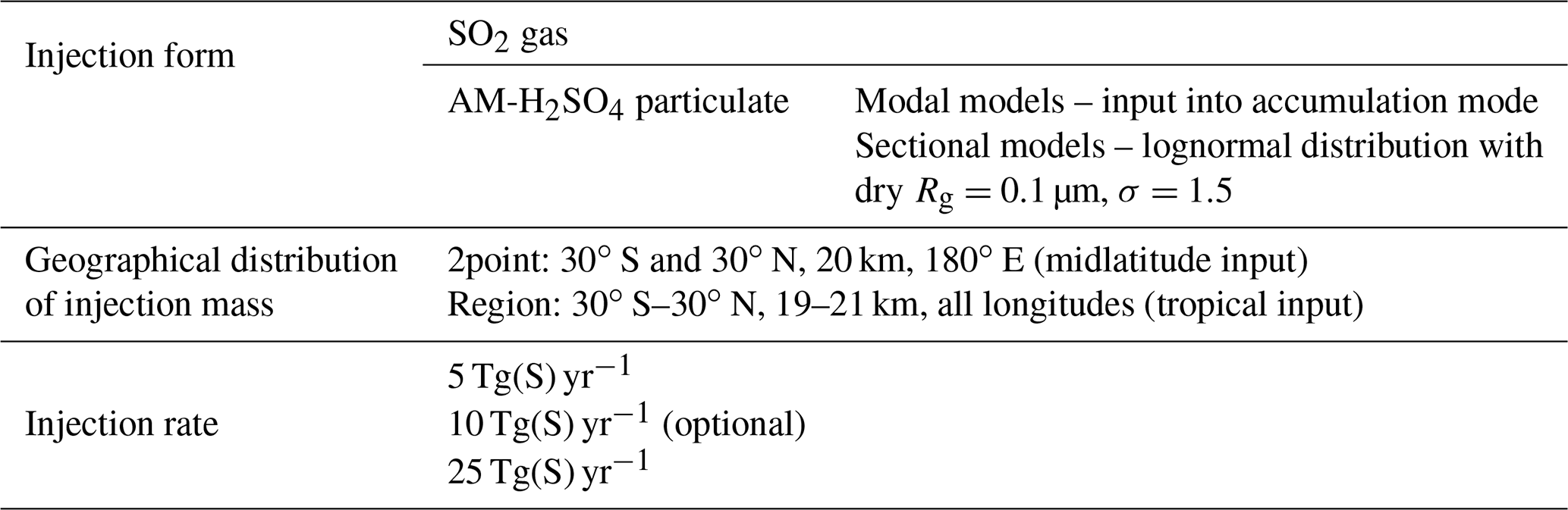
Two different geographical distributions of injection mass were chosen: either uniformly distributed in a broad tropical region between 30∘ S and 30∘ N, with a 2 km thickness centred around 20 km, and across all longitudes (hereinafter called regional injections), or narrowly injected at two model grid points located at 30∘ S and 30∘ N, at 20 km (CESM2 and SOCOL-AER) or 18–20 km (MAECHAM5-HAM) and at 180∘ E longitude (hereinafter called 2point injections) outside the tropics. The regional injections are designed to utilize the Brewer–Dobson circulation to distribute emissions globally and maximize their residence time, as has been observed for volcanic aerosol clouds (Dyer and Hicks, 1968; Grant et al., 1996). The 2point injections occur outside the tropical stratospheric reservoir (Grant et al., 1996; Tilmes et al., 2017) and are meant to concentrate geoengineering impacts at higher latitudes and to explore microphysical differences when injections are more concentrated spatially. All models simulated injections of 5 and 25 Tg(S) yr−1, and the MAECHAM5-HAM and SOCOL-AER models also simulated a 10 Tg(S) yr−1 injection. The combination of two injection forms, two geographical distributions of injection mass and two (or three) injection rates yielded 8 (or 12) perturbation scenarios. The same set of model calculations (excluding SOCOL-AER due to lack of an internally generated QBO) has been analysed for changes in the QBO by Franke et al. (2021).
We analyse changes in global aerosol properties and radiative forcing to determine whether the use of AM-H2SO4 can increase (compared to SO2) the radiative efficacy per unit of material injected across a range of models. If so, can this be attributed to increased stratospheric lifetime of the aerosols, improved scattering efficacy or some other factor? What contributes to inter-model differences, and what can these differences tell us about uncertainty in the response to the aerosol injections? Finally, we examine some of the side effects of increasing stratospheric aerosol and explore how they differ with AM-H2SO4 versus SO2 injection and with geographical distribution of injection mass.
3.1 Changes in global aerosol properties
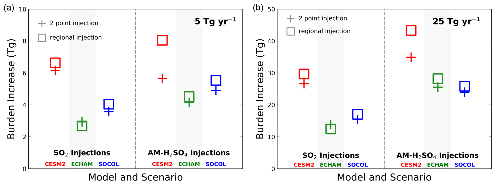
Figure 1Global sulfuric acid aerosol burden increase (90∘ S–90∘ N; stratosphere and troposphere) in Tg of sulfur due to geoengineering injection of (a) 5 Tg(S) yr−1 and (b) 25 Tg(S) yr−1. Panels (a) and (b) show the three models, CESM2 in red, MAECHAM5-HAM (labelled ECHAM) in green and SOCOL-AER in blue, with the left side of each panel representing injection as SO2 and the right side of each panel representing injection as accumulation-mode H2SO4. Square symbols represent injection into a region around the Equator from 30∘ S to 30∘ N, 19–21 km and all longitudes. Plus symbols represent injection into two model grid points at 30∘ S and 30∘ N, 20 km and 180∘ E longitude.
We start by examining the aerosol burden using the global (troposphere and stratosphere) rather than stratospheric burden to reduce uncertainties that would arise from inconsistent diagnoses of tropopause height and because the troposphere represents less than 10 % of the total burden increase in our scenarios. Injections of 5 Tg(S) yr−1 in the form of SO2 yield increases in the global aerosol burden of 2.7 to 6.6 Tg of sulfur while injections of 5 Tg(S) yr−1 as AM-H2SO4 yield increases in aerosol burden of 4.2 to 8.1 Tg of sulfur (Fig. 1). Accumulation-mode particle injection produces a larger burden increase than SO2 injection in all cases except for the CESM2 model using 2point injections of 5 Tg(S) yr−1. Inter-model differences are roughly a factor of 2 larger than difference between SO2 and AM-H2SO4. Differences arise in part from dynamics including the QBO which may influence microphysics by changing tropical confinement (Visioni et al., 2018b). The CESM2 model in all cases shows the highest burden increases and the MAECHAM5-HAM model the lowest in most cases. The SOCOL-AER model, with the same dynamical core as the MAECHAM5-HAM model, produces burden increases closer to that model than to CESM2. For 25 Tg(S) yr−1 injections, most results scale proportionately, though in this case the MAECHAM5-HAM model produces a larger burden than SOCOL-AER with AM-H2SO4 injections. A previous intercomparison of geoengineering results between the MAECHAM5-HAM and CESM2 models (Niemeier et al., 2020) found significantly larger aerosol burden increases for equatorial injection of SO2 with CESM2 than with MAECHAM5-HAM and attributed the greater CESM2 burden to greater vertical advection in the CESM2 model. Differences in global aerosol burden due to the chosen geographical distribution (2point or region) are modest except with the CESM2 model injecting AM-H2SO4. In most cases, regional injections produce slightly greater global burdens.
Figure 2 shows the zonal mean of vertically integrated aerosol mass increase (troposphere and stratosphere) as a function of latitude relative to the reference scenario for each model. Significant increases in aerosol column burden are seen at all latitudes for all scenarios; however, the latitudinal pattern is different for regional and 2point injections. Regional injections which evenly spread the injection mass in a region centred around the Equator between 30∘ S and 30∘ N result in aerosol column burden peaks over the Equator and at 45∘ N and 45∘ S, and minima at 30∘ S and 30∘ N at the subtropical barrier zone (see, e.g. Strahan and Douglas, 2004). The 2point injections at 30∘ S and 30∘ N show minimal increases in aerosol column burden at the Equator and maximum aerosol column increases at about 45–50∘ S and 45–50∘ N. The hemispheres differ due to the stronger polar vortex in the Southern Hemisphere that inhibits mixing of midlatitude and polar air resulting in a strong contrast between the two regions in this hemisphere. Of these two geographical distributions of injection mass, the regional injections (30∘ S–30∘ N) yield more uniform global distributions of aerosol, whereas the 2point injections at 30∘ S and 30∘ N concentrate more aerosol at midlatitudes and high latitudes which could concentrate geoengineering effects toward the high latitudes which are warming fastest. Figure 2 explains the significant differences in total burden between the 2point and regional injections of AM-H2SO4 seen in the CESM2 model in Fig. 1 as a strong subtropical barrier minimizing the impact of extratropical injections on the tropics and tropical upwelling enhancing the impact of tropical injections in the same region. Because SO2 injections yield larger particle sizes, the tropical upwelling has less impact on the aerosol burden in that case. The MAECHAM5-HAM and SOCOL-AER models, which share the same dynamical core, have weaker subtropical barriers.
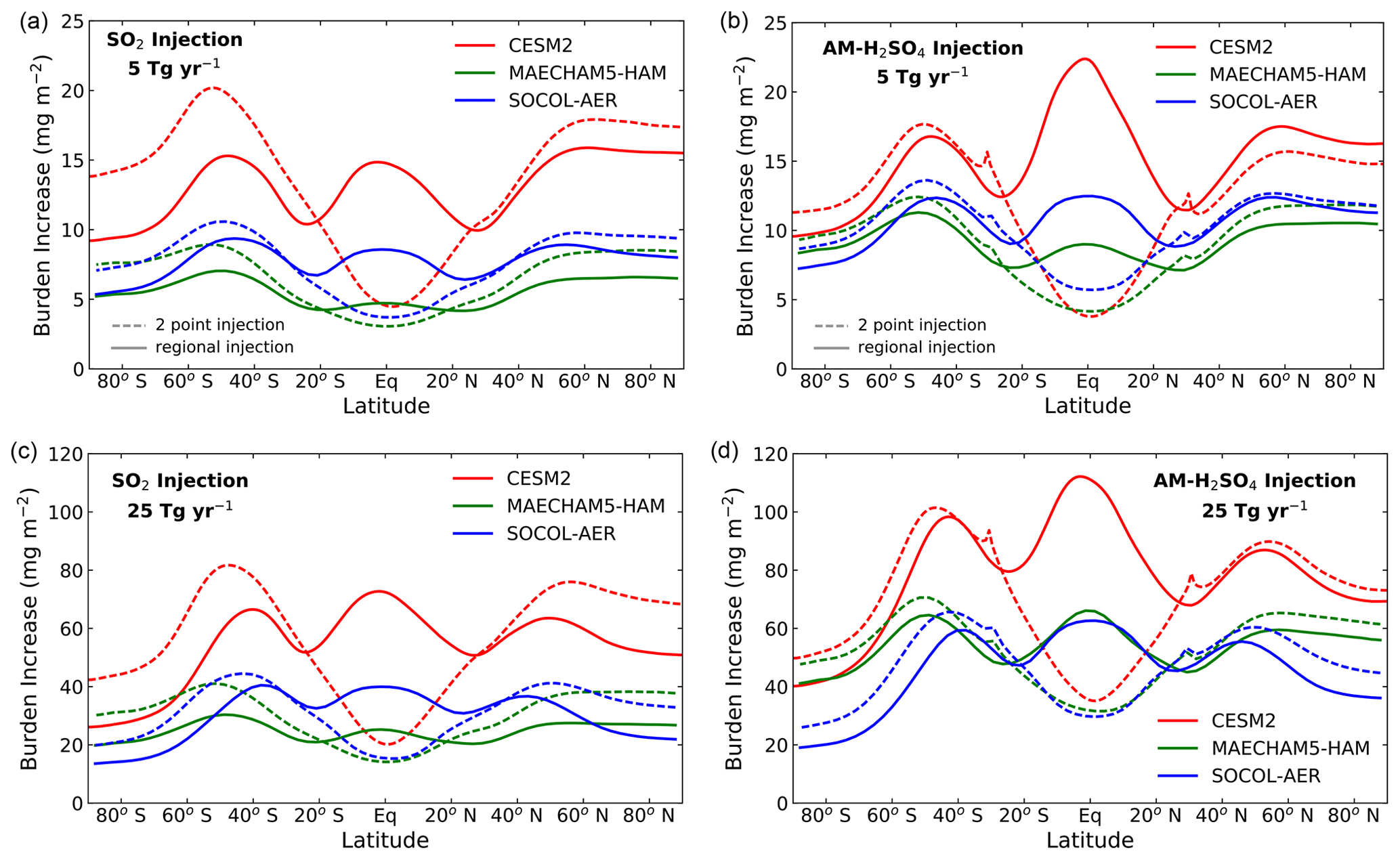
Figure 2Zonal mean aerosol column burden increase above background (mg m−2) with 5 Tg(S) yr−1 injections (a, b) and 25 Tg(S) yr−1 injections (c, d) as a function of latitude for SO2 injections (a, c) and AM-H2SO4 injections (b, d). Regional injections are shown with solid lines and 2point injections with dashed lines.
The global aerosol burdens normalized by the injection rate are shown in Fig. 3 as a function of injection rate. The normalized burden has units of time and can be considered the residence time of injected sulfur, which varies from 0.5 to 1.3 years for SO2 injections and from 0.8 to 1.7 years for AM-H2SO4 injections. Regional injections have longer residence time than 2point injections in most cases. The CESM2 model shows longer residence times than the other models, consistent with its greater burdens. The SO2 injections (Fig. 3, left panel) all show decreasing residence time with increasing injection rate. This is consistent with other studies (Niemeier and Timmreck, 2015; Heckendorn et al., 2009) showing decreasing injection efficiency with increasing injection amount, which has been found to result from substantial increases in mean particle size and thus sedimentation rates. However, injections of AM-H2SO4 (Fig. 3, right panel) show increasing residence time with increasing injection for the CESM2 and MAECHAM5-HAM models. The AM-H2SO4 scenarios were designed to minimize the growth in average particle size as a function of injection rate, since sulfur is added to each grid box as particles of approximately 0.1 µm radius which grow mainly by coagulation. In addition, aerosol heating in the tropical lower stratosphere increases the strength of the Brewer–Dobson circulation, resulting in greater lofting in the tropical stratosphere. For accumulation mode and smaller particles, (Niemeier et al., 2020), lofting can prolong the residence time for 25 Tg(S) yr−1 injections relative to 5 Tg(S) yr−1 injections, though the details of this process are model dependent and include changes in the QBO for the CESM2 and MAECHAM5-HAM models (Franke et al., 2021). The SOCOL-AER model, which uses a sectional aerosol scheme, may transfer aerosol mass into larger particle sizes more efficiently than the two modal models and thus yield more sedimentation at higher loadings.
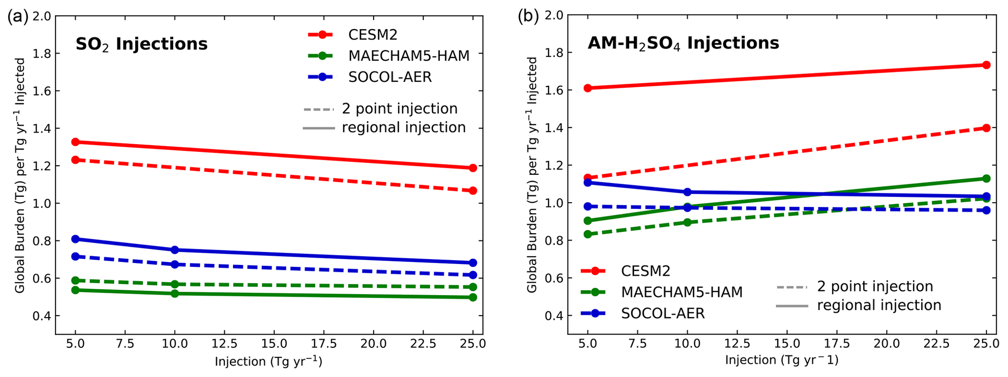
Figure 3Increase in global sulfuric acid aerosol burden normalized by geoengineering injection rate in units of Tg(S) per (Tg(S) yr−1) as a function of injection rate. The y axis also represents the residence time in years of injected sulfur as aerosol. SO2 injections (a) show decreasing residence time with increasing injection rate, whereas AM-H2SO4 injections (b) show increasing residence time with increasing injection rate for the CESM2 and MAECHAM5-HAM models. Regional injections (solid lines) show longer residence times than 2point injections (dashed lines) in most cases.
Globally averaged effective wet radius (Reff) at 60 hPa near the injection region and where these values maximize is shown in Fig. 4 (left panel) for background conditions and for injections of 5 and 25 Tg(S) yr−1 of SO2 or AM-H2SO4. The effective radius at 60 hPa after continuous injection of AM-H2SO4 results in Reff from 0.27 to 0.39 µm with 5 Tg(S) yr−1 injections, whereas SO2 injections yield Reff of 0.40 to 0.52 µm for the same annual sulfur injection. The SO2 injections consistently yield larger average particles than the AM-H2SO4 injections. As has been seen in other studies (English et al., 2012; Vattioni et al., 2019), injection of SO2 results in substantial particle size growth since most of the injected sulfur condenses onto the larger existing particles or nucleates and preferentially coagulates onto the larger background particles. The assumed lognormal size of the input AM-H2SO4 particles in our scenarios is equivalent to a wet Reff of 0.18 µm (0.16 for MAECHAM5-HAM) and the additional particle growth is due to coagulation with both background and other injected particles. For 5 Tg(S) yr−1 injections of AM-H2SO4 particles, the resulting global averaged Reff at 60 hPa is within or smaller than the optimal Reff for scattering (blue band in the figure), whereas the Reff resulting from SO2 injections is larger than optimal for scattering, particularly for regional injections. Increasing the injection rate from 5 to 25 Tg(S) yr−1 results in larger mean particles in all cases, with the SO2 injection scenarios responding more strongly than the AM-H2SO4 scenarios. The MAECHAM5-HAM model shows only small increases in Reff for the AM-H2SO4 scenarios as a function of injection rate. The SO2 injection scenarios all produce larger Reff with regional injections, while the AM-H2SO4 injection scenarios produce larger Reff with 2point injections. Based on injection location and aerosol lifetime alone, we would expect the regional injections into the tropical stratospheric reservoir to produce larger particles in all cases.
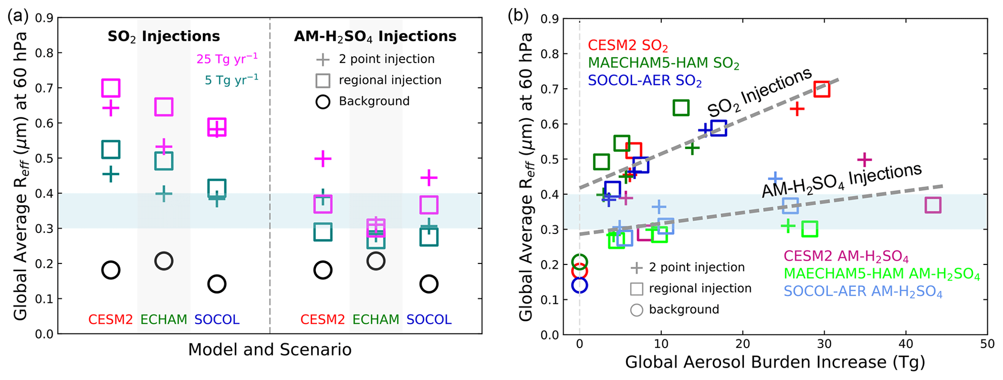
Figure 4Global average effective radius (µm) at 60 hPa (a) for the three models with SO2 injections of 5 and 25 Tg(S) yr−1 (left side) and with AM-H2SO4 injections of 5 and 25 Tg(S) yr−1 (right side). Scatter plot of global average effective radius (µm) at 60 hPa plotted against the global increase in aerosol burden in Tg(S) (b). Regression lines are shown for both SO2 (R2=0.74) and AM-H2SO4 (R2=0.34) injections. Injections into regions are shown by open squares, while injections at two points are shown with plus symbols and for background conditions with open circles. The light blue shaded region represents the optimal effective radius for scattering of solar radiation assuming a lognormal distribution and σ between 1.1 and 1.8 (John Dykema, personal communication, 2019).
Figure 4 (right panel) shows the same Reff parameter at 60 hPa plotted against the increase in global aerosol burden for each case, including the 5, 10 and 25 Tg(S) yr−1 scenarios. Linear regression lines are plotted for SO2 injections and AM-H2SO4 injections (equal weighting of plotted points for all models), showing that the relationship between burden and Reff is close to linear though more steeply sloped for SO2 injections. R2 values are 0.74 for SO2 injection and 0.34 for the AM-H2SO4 injections. SO2 injection cases all lie above the AM-H2SO4 injection cases, with the latter yielding smaller Reff and larger burden for the same annual injection amount and even greater burdens with similar Reff values. The MAECHAM5-HAM model exhibits a somewhat flatter regression slope than the other models with AM-H2SO4 injections (smaller sensitivity of Reff to burden) and an upward offset on the regression line with SO2 for regional injections.
Particle size distributions for the 30∘ S–30∘ N region at 60 hPa are shown in Fig. 5 for SO2 injections (left panels) and AM-H2SO4 injections (right panels) of 5 Tg(S) yr−1. Note that the CESM2 model includes only three sulfuric acid aerosol modes, omitting the nucleation mode and transferring the mass of freshly nucleated particles into the Aitken mode. The SO2 injection scenarios result in an increase in nucleation-mode particles relative to background levels (dotted lines in Fig. 5) in the MAECHAM5-HAM model, particularly with regional injections in the tropics and a decrease in the nucleation mode in the SOCOL-AER model. In these scenarios, the SOCOL-AER model results reflect a predominance of condensation, while the MAECHAM5-HAM results reflect a larger role for nucleation. An analysis with the SOCOL-AER model revealed that concentrations of nucleation-mode particles are sensitive to the order of calculation of nucleation and condensation, the time-splitting scheme and the time step, though this does not affect conclusions concerning the overall differences between SO2 and AM-H2SO4 injections.

Figure 5Size distributions (dd10log R, particles cm−3 µm−1) averaged between 30∘ S and 30∘ N at 60 hPa for the three models with SO2 (a, c) and AM-H2SO4 (b, d) injections of 5 Tg(S) yr−1 and with 2point injections (a, b) and regional injections (c, d). Background size distributions are shown as dotted lines.
Large increases in the accumulation mode and coarse mode are seen for all models with SO2 injection. The coarse modes have mode radii values (Rg) of 0.4 to 0.7 µm, with MAECHAM5-HAM having the smallest coarse mode Rg but also the smaller background distribution in the coarse mode. AM-H2SO4 injections decrease the nucleation-mode and Aitken-mode particles as many of these particles are scavenged by the injected accumulation-mode particles. Coagulation with background particles and with other injected particles moves the accumulation-mode particle size distribution from an Rg of 0.1–0.12 µm upon injection to 0.2–0.3 µm for the CESM2 and SOCOL-AER models with 2point injections, while the MAECHAM5-HAM model retains a mode at 0.1 µm and also grows the coarse mode at 0.3 µm. The size distributions with regional injections of AM-H2SO4 tend to maintain a mode close to the accumulation-mode injection size.
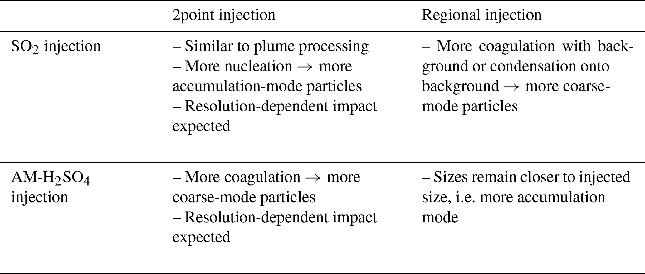
The size distributions respond differently to 2point rather than regional injections depending on whether SO2 gas or AM-H2SO4 particulate is injected. These results suggest the way aerosol microphysics drives differences between AM-H2SO4 and SO2 injection scenarios (see Table 3). For AM-H2SO4, 2point injections produce larger Reff (Fig. 4) and smaller global burdens (Fig. 1) than regional injections. The regional AM-H2SO4 injection cases have size distributions (see Fig. 4) which remain closer to their injected size distributions. We expect that injection of AM-H2SO4 into points increases the coalescence rate, driving the radius up and the lifetime down due to sedimentation of large particles. In contrast, SO2 regional injections yield larger coarse-mode particle sizes than the 2point injections, resulting in a larger Reff. The 30 d conversion time from SO2 to H2SO4 leads to H2SO4 condensation onto existing background particles that favours coarse-mode growth, particularly with dispersed regional injections. Small freshly nucleated particles in this scenario preferentially coagulate with the larger background particles, also favouring coarse-mode growth. Point injections of SO2 are more likely to create locally high densities of nucleation-mode particles that would coagulate among themselves, thus lowering the average size relative to regional injections. This effect is somewhat akin to injections into an aircraft plume but on a very different scale. We expected this effect will be strongly dependent on model resolution which may partly explain the model discrepancies. Given our chosen scenarios, some of the differences between regional and 2point injections are likely due to the interaction of dynamics with injection location – injections outside the tropics will less efficiently be transported in the upward branch of the Brewer–Dobson circulation, which could lead to faster stratospheric removal and lower global burdens for 2point injections.
Table 3Matrix explaining 2point vs. regional injection effects.
3.2 Changes in radiative forcing and stratospheric temperature

Figure 6Globally averaged change in net top-of-atmosphere shortwave and longwave radiative forcing (W m−2) due to geoengineering injection of (a) 5 Tg(S) yr−1 and (b) 25 Tg(S) yr−1. Colours and symbols are as in Fig. 1.
Changes in the top-of-atmosphere (TOA) radiative forcing (RF) of shortwave (SW, solar) and longwave (LW, thermal) bands combined are shown in Fig. 6 for our simulations with 5 and 25 Tg(S) yr−1 injections under all-sky conditions. RF changes range from −0.9 to −2.5 W m−2 with SO2 injections of 5 Tg(S) yr−1 and from −1.6 to −3.8 W m−2 with AM-H2SO4 injections of 5 Tg(S) yr−1. For comparison, approximately −4 W m−2 forcing would be needed to offset a doubling of CO2 (Etminan et al., 2016). Inter-model differences encompass a factor of 3 and are larger than differences due to injection form (AM-H2SO4 vs. SO2) and geographical distribution of injection mass (2point vs. regional) in the 5 Tg(S) yr−1 case (left panel), but differences due to injection form are of a similar magnitude as inter-model differences with 25 Tg(S) yr−1 (right panel). The efficacy (RF reduction per Tg of sulfur injected annually) is shown in Fig. 7 as a function of injection rate. The efficacy is reduced with increasing injection rate for SO2 injection scenarios, a consequence of the larger particles generated at high injection rates that both increase sedimentation and decreases the shortwave scattering efficiency, which is consistent with previous studies (Heckendorn et al., 2009; Kleinschmitt et al., 2018). Efficacy is also reduced with increasing injection rate for AM-H2SO4 injections with the SOCOL-AER model but stays roughly constant with injection rate in the CESM2 (2point injection only) and MAECHAM5-HAM models. Even though the normalized aerosol burden increases with increasing AM-H2SO4 injection rate for these models (Fig. 2), the RF efficacy is insensitive to injection rate, possibly due to the offsetting effects of aerosol heating on circulation and stratospheric water vapour and more modest changes in particle size.
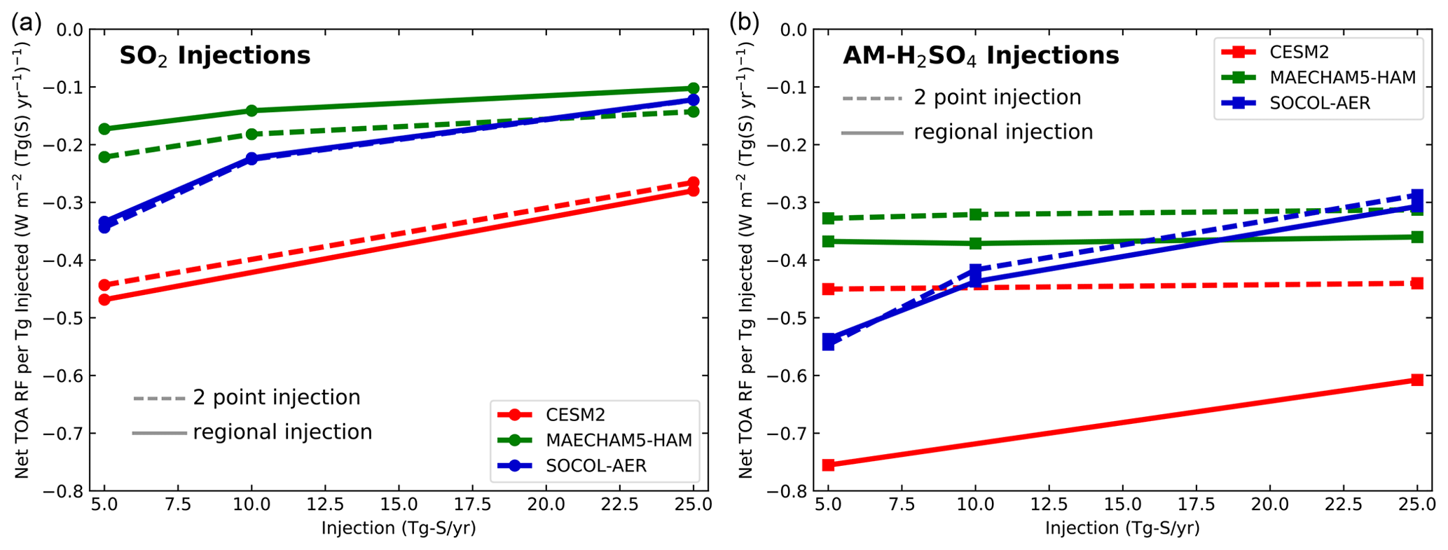
Figure 7Globally averaged change in net top-of-atmosphere shortwave and longwave radiative forcing (W m−2) per unit annual injection (Tg(S) yr−1) due to geoengineering injection as a function of injection rate for (a) SO2 injections and (b) AM-H2SO4 injections.
Figure 8 shows a scatter plot of the change in SW and LW TOA RF plotted against the increase in global aerosol burden. The upper left panel of Fig. 8 expands the region from 0 to 18 Tg(S) burden increase. Linear regression lines for the SO2 injections and AM-H2SO4 injections are shown, with R2 values greater than 0.9 in both cases, indicating that global burden is a good predictor of change in TOA RF. For the same burden increase, the AM-H2SO4 injection scenarios show somewhat greater RF changes than the SO2 injection scenarios, which we can attribute to a more optimal size distribution after AM-H2SO4 injections. Model differences in RF are, for the most part, contained in the differences in calculated burdens, with differences in size distributions yielding different linear fits for SO2 vs. particulate injection, consistent with results for Reff.
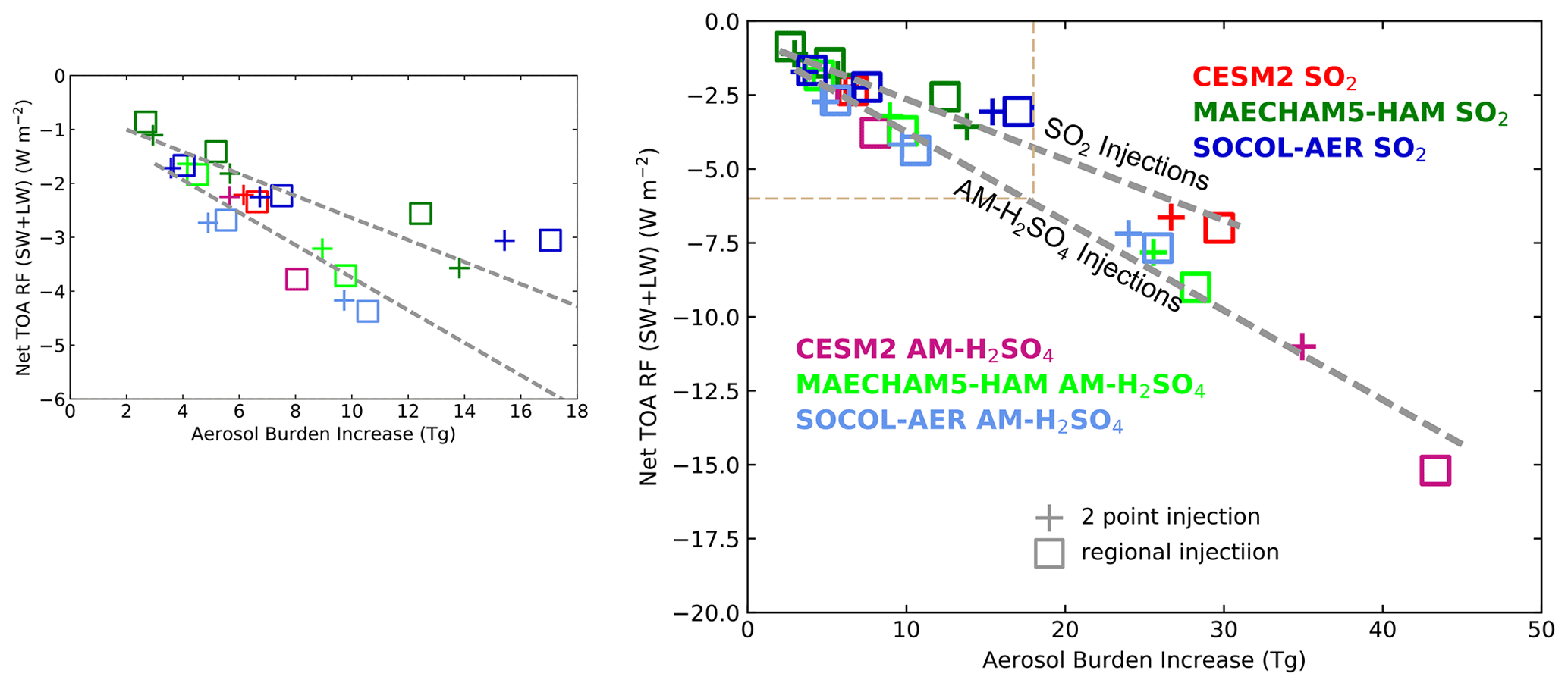
Figure 8Scatter plot of globally averaged net top-of-atmosphere shortwave and longwave radiative forcing (W m−2) due to geoengineering injection relative to the corresponding increase in global aerosol burden (Tg(S)). The smaller left panel is a finer scale for the upper left corner of the main plot. Regression lines are shown for SO2 injections (R2=0.93) and for AM-H2SO4 injections (R2=0.98).
Figure 9 shows the latitudinal variation in net TOA SW and LW radiative forcing for both 5 and 25 Tg(S) yr−1 injections. The MAECHAM5-HAM model shows less variability of RF with latitude than the other models, while the CESM2 model shows much more variability. The SOCOL-AER model shows near-zero RF change, and sometimes positive RF change, in the high latitudes. The 2point injections in most cases produce greater RF change at midlatitudes and high latitudes as expected, while the regional injections produce a much greater impact on RF in the tropics. Compared to latitudinal changes in aerosol burden (Fig. 3), changes in RF exhibit more small-scale variability, a result of the high variability in tropospheric cloudiness.
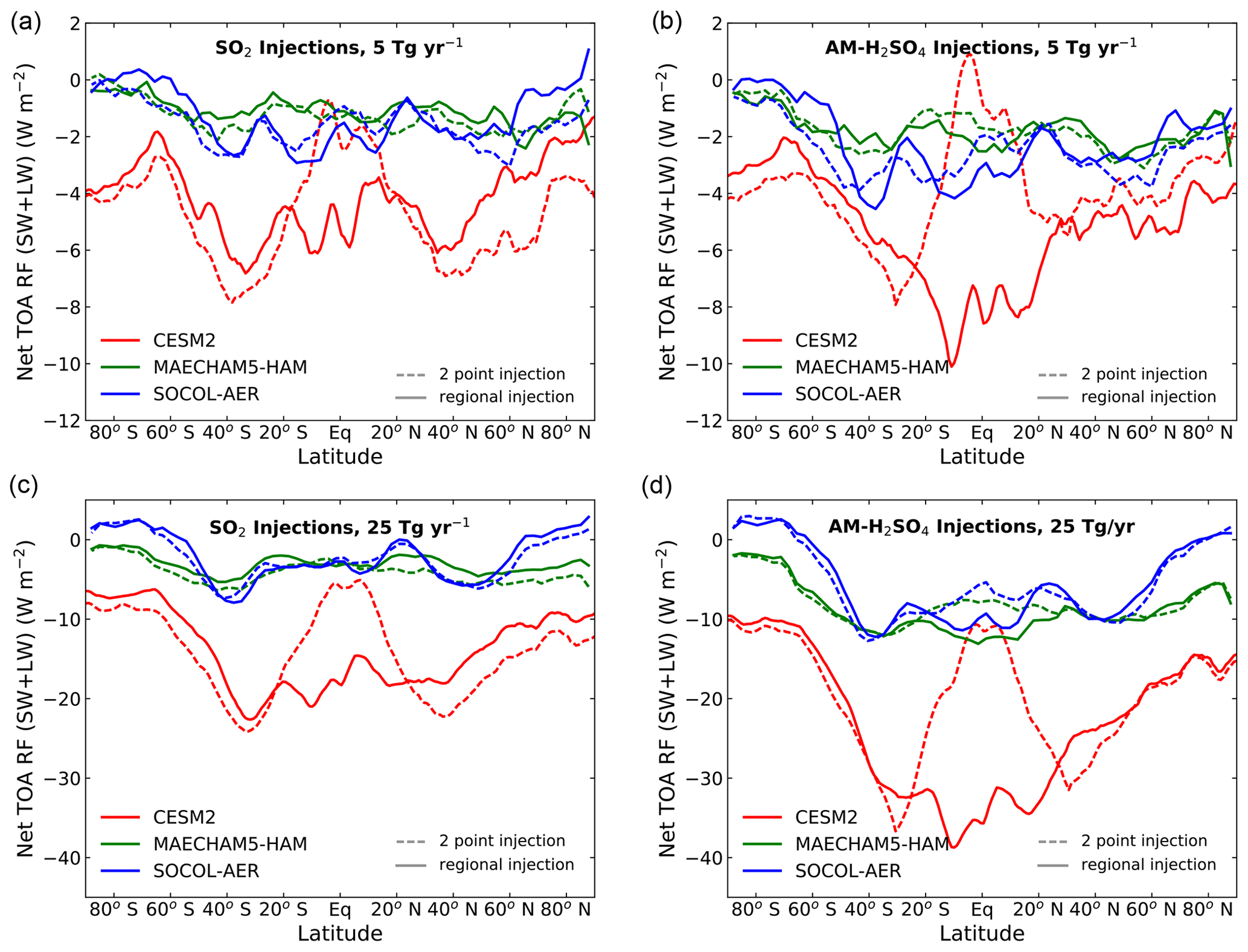
Figure 9Zonal mean net top-of-atmosphere shortwave and longwave radiative forcing (W m−2) with 5 Tg(S) yr−1 injections (a, b) and 25 Tg(S) yr−1 injections (c, d) as a function of latitude for SO2 injections (a, c) and AM-H2SO4 injections (b, d).
Next, we look at the vertical profiles of changes in tropical temperature (30∘ S–30∘ N) in Fig. 10. Sulfuric acid aerosols absorb in the longwave and lead to atmospheric heating, which would lead to an enhancement in the Brewer–Dobson circulation and to increased transport of H2O into the stratosphere. Increased stratospheric water vapour could lead to ozone losses via an enhanced HOx cycle in the upper stratosphere (Tilmes et al., 2018). Thus, aerosol heating in the tropical lower stratosphere is considered a serious risk of geoengineering. Previous studies indicate that such stratospheric changes could impact tropospheric climate (Simpson et al., 2019; Jiang et al., 2019), though we do not explore that here. Maximum model-calculated temperature changes in this region range from 1.7 K for the MAECHAM5-HAM model to 5.3 K for the CESM2 model with SO2 injections of 5 Tg(S) yr−1. With AM-H2SO4 injections of the same magnitude, model-calculated tropical temperature changes range from 2.1 to 6.4 K for the same two models. The SOCOL-AER model results are similar to the CESM2 model results with SO2 injections of the same magnitude and geographic distribution (2point vs. region), though this similarity does not extend to AM-H2SO4 injections. The larger temperature changes with AM-H2SO4 likely reflect the greater stratospheric burden for the same sulfur injection amount, a result seen in all three models (Fig. 1).
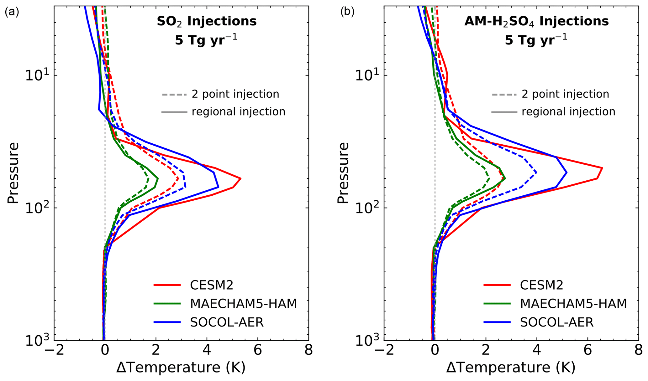
Figure 10Change in atmospheric temperature (K) averaged between 30∘ S and 30∘ N due to 5 Tg(S) yr−1 of geoengineering injection as a function on height for (a) injections of SO2 and (b) injections of AM-H2SO4.
In Fig. 11, we look at the changes in H2O and changes in temperature at 90 hPa in the tropics, shown as a scatter plot including injections of 5, 10 and 25 Tg(S) yr−1. A value of 90 hPa is close to the cold-point temperature which determines H2O concentration entering the stratosphere, though the actual cold point could vary from model to model and from low to high injection rates. MAECHAM5-HAM results are not shown as H2O was not calculated diagnostically in this model. Plotting H2O against temperature shows that 90 hPa tropical water vapour mixing ratio is determined by 90 hPa tropical temperature, though with different relationships for the SOCOL-AER and CESM2 models. Since we plot these quantities averaged over time and spatial volumes, they do not follow the Clausius–Clapeyron equation but fall below it. Compared to control runs with H2O values of about 4 ppmv in the tropics at this altitude, injections of 25 Tg(S) yr−1 of SO2 or AM-H2SO4 yield H2O increases of 3.7 to 12 ppmv, which represents increases of factors of 2–4. The SOCOL-AER model has larger increases in 90 hPa water vapour per degree of heating than the CESM2 model. As the H2O vapour crossing the 90 hPa surface in the tropics largely determines H2O concentrations throughout the stratosphere, this would be expected to significantly perturb stratospheric chemistry and ozone.

Figure 11Scatter plot of water vapour change (ppmv) relative to change in temperature (K) at 90 hPa and averaged between 30∘ S and 30∘ N for injections of 5, 10 and 25 Tg(S) yr−1 of SO2 or AM-H2SO4. Results from CESM2 and SOCOL-AER only are shown, as the MAECHAM5-HAM model used fixed H2O.
3.3 Chemical changes
Increases in stratospheric water vapour concentration are expected to modify OH concentration in the stratosphere as well. However, OH chemistry is complex and HOx cycles interconnect with those of NOx, ClOx and BrOx. The CESM2 and SOCOL-AER models show significant increases in tropical OH concentration above 50 hPa, up to a 15 % increase for SOCOL-AER and a 10 % increase for CESM2 with 5 Tg(S) yr−1 injection. These relative increases in OH are consistent with relative increases in H2O at 90 hPa. Analysis of our SO2 injection scenarios shows that 7 %–10 % of the additional global sulfur (SO2 + H2SO4) burden remains as SO2 in the SOCOL-AER model, 5 %–8 % in the CESM2 model and 20 %–22 % for MAECHAM5-HAM. Derived residence times of the excess SO2 burden (burden/SO2 injection rate) are 18–28 d for SOCOL-AER, 25–37 d for CESM2 and 50–60 d for MAECHAM5-HAM. The long residence time for the MAECHAM5-HAM model results from the prescribed OH field employed in these calculations. SO2 residence times in all models change very little with injection rate from 5 to 25 Tg(S) yr−1, indicating that OH is not depleted by these large continuous injections of SO2, as this effect is counterbalanced by increases in stratospheric H2O due to heating of the tropical tropopause region.
Next, we evaluate the impacts on ozone, which are shown as zonal mean total ozone column (TOC) changes as a function of latitude in Fig. 12 for the 5 Tg(S) yr−1 case for the two models which include HOx chemistry (SOCOL-AER and CESM2). In agreement with previous studies (Pitari et al., 2014; see their Fig. 14c), we find that SO2 injections lead to a TOC decrease, which maximizes in midlatitudes and high latitudes. However, we find larger polar losses in the Southern Hemisphere (20–30 DU) because of the larger sulfur injections in our study (5 vs. 2.5 Tg(S) yr−1 in their study). Most of the column depletion occurs because of changes in the lower stratosphere, where the primary mechanism is N2O5 hydrolysis and consequent formation of nitric acid (HNO3), thus decreasing ozone loss due to NOx cycles and increasing it due to ClOx and HOx cycles. In addition, chlorine is activated via heterogeneous reaction of ClONO2 and H2O on stratospheric aerosols, contributing to most of the ozone depletion in polar latitudes. Both chemical pathways are enhanced via enhanced aerosol burden and consequently greater surface area density (SAD). The impact of chlorine on ozone is a function of the simulation year (2040) and future projection chosen, with our 2040 simulations containing 2.4 ppbv of total chlorine. Changes in dynamics, such as increased tropical upwelling (and consequent tropical lower stratospheric ozone decreases), modified stratosphere–troposphere exchange and chemical changes such as OH increases (and consequent enhancement of HOx depletion cycles), also contribute to ozone changes.

Figure 12Change in zonal average column ozone (Dobson units) due to geoengineering injection as a function of latitude for (a) 5 Tg(S) yr−1 of SO2 injection and (b) 5 Tg(S) yr−1 of AM-H2SO4 injection.
Ozone decreases in the lower stratosphere are partly offset by ozone increases in the middle stratosphere (10–50 hPa), due to weakened NOx depletion cycles, in agreement with other studies (Heckendorn et al., 2009). As atmospheric chlorine concentrations decrease into the future and N2O emissions continue, NOx-mediated depletion will become dominant (Ravishankara et al., 2009) and the impact of increasing sulfuric acid aerosol on ozone is expected to become predominantly positive. The CESM2 model, in fact, shows increases in total ozone poleward of 30∘ N with regional injections of SO2 in 2040. AM-H2SO4 injections lead to a very similar TOC pattern as SO2 injections in both models, although depletions are slightly larger (by 10 %–20 %) with AM-H2SO4 due to larger sulfuric acid aerosol burdens (Fig. 1) with smaller mean particle size and consequently larger SAD throughout the stratosphere. Hence, more surface area is available for heterogeneous reactions, leading to larger ozone depletion in the case of AM-H2SO4 rather than SO2 injections, consistent with previous findings (Vattioni et al., 2019). Note that while the CESM2 model has larger increases in aerosol burden than the SOCOL-AER model, it nevertheless shows smaller changes in total ozone.
Geoengineering by stratospheric sulfur injection can have a strong impact on Arctic and Antarctic ozone depletion (Tilmes et al., 2009). However, this effect is generally less severe in the Arctic and is strongly modulated by interannual variations in the polar vortex strength. Both models produce Antarctic ozone depletion of 20–35 DU, while the Arctic shows smaller depletion (up to 18 DU) for SOCOL-AER. The CESM2 model shows minimal Arctic ozone depletion (up to 8 DU) for most cases but an increase in Arctic column ozone with SO2 regional injections where positive changes in the middle stratosphere dominate negative changes in the lower stratosphere. Longer simulations than those considered here (8 years) would be needed to robustly detect dynamical and chemical effects on the Arctic stratosphere.
Figure 13 shows the correlation between global ozone change and global aerosol burden (left panel) or net TOA RF (right panel). Changes in total ozone column are a mix of both positive and negative local changes, and the global average includes large depletions in the Antarctic and small-to-moderate depletions elsewhere. The correlations with burden and net TOA RF are fairly compact for the SOCOL-AER model (R2=0.95 for burden, 0.90 for RF) but less so for the CESM2 model (R2=0.58 for burden, 0.72 for RF) which is much more sensitive to injection form and location. Regression lines for the SOCOL-AER model are much steeper than those for the CESM2 model, indicating different ozone sensitivities in the two models. A −4 W m−2 change in net TOA RF corresponds to global ozone changes of from −1.5 % to −5 % among our two models and four injection scenarios, indicating large model uncertainties in ozone response to SRM.
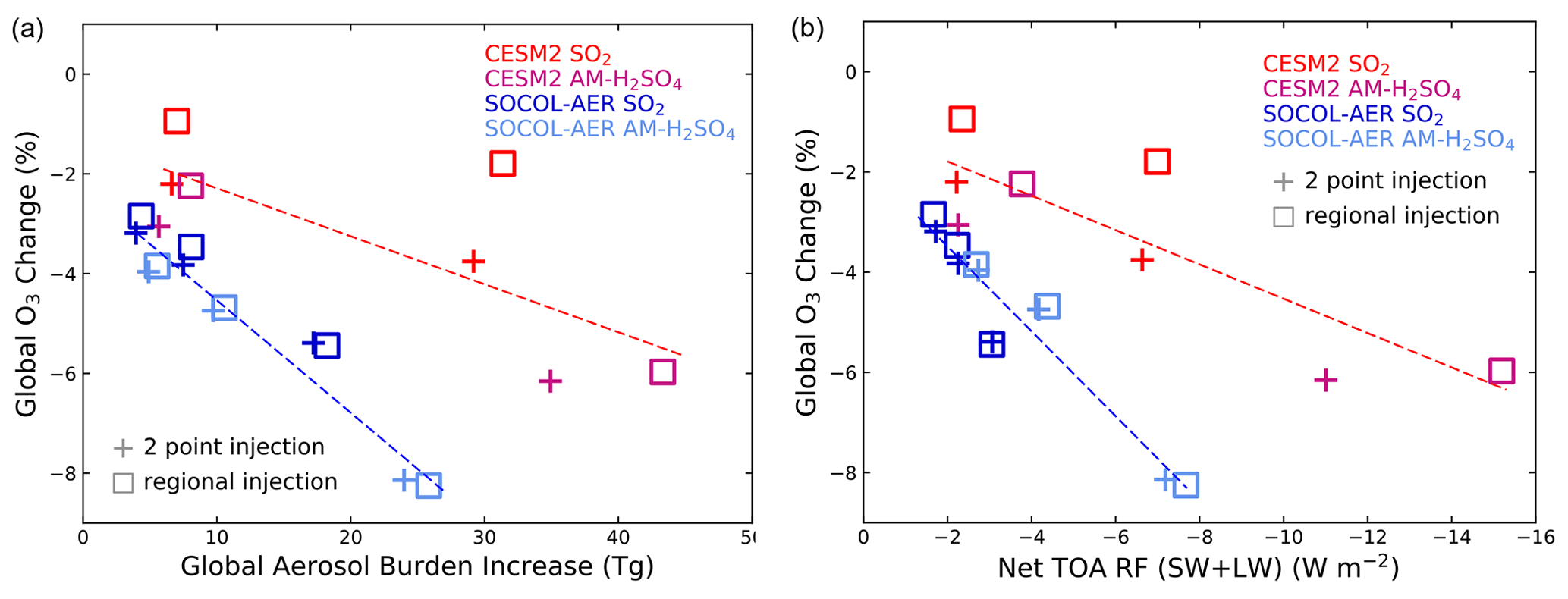
Figure 13Global average change in column ozone (%) due to geoengineering injection plotted against (a) the global average aerosol burden increase (Tg(S)) and (b) the global average change in SW and LW radiative forcing (W m−2). Regression lines are shown for each model with R2 values of 0.95 and 0.90 for SOCOL-AER (burden and RF, respectively) and 0.58 and 0.72 for CESM2.
Most obviously, the fact that all three models show that use of AM-H2SO4 particles can aid in controlling the large-scale particle size distribution strengthens the case that this method might be useful for sulfuric acid aerosol SRM. Improved control of particle size can, in turn, allow use of less sulfur to achieve the same radiative forcing, or it could allow higher levels of radiative forcing with less nonlinear saturation. Our three-model intercomparison increases the confidence in this general result while simultaneously demonstrating the significant uncertainty that arises from differences in model dynamics and model treatment of aerosol microphysics and chemistry. We note first there are large inter-model differences in both absolute quantities such as aerosol burden and radiative forcing and in derivative quantities such as aerosol lifetime and the change in radiative forcing with injection rate. Nevertheless, the intra-model differences in the impact of SO2 vs. AM-H2SO4 show systematic agreement among the models. The inter-model differences in radiative forcing and Reff are consistent with the inter-model differences in aerosol burden as diagnosed by the compact relationships among these quantities. And the significant difference in correlation slopes between SO2 and AM-H2SO4 injection scenarios indicates that the different size distributions resulting from the different injection forms also play a significant role in determining the radiative forcing and radiative forcing per unit of injected mass flux, i.e. RF efficacy.
Perhaps the most interesting result is the systematic differences in radiative efficacy achieved over the 2×2 matrix of cases formed by the choice of SO2 vs. AM-H2SO4 and regional vs. 2point injections, which are summarized in Table 3. These results hint at the limitations that come from the unresolved spatial scales between the injection plume and the model grid boxes, limitations that are common to these three models along with all other global models that have been used for studying SRM. For AM-H2SO4, 2point injections produce larger particles and lower radiative efficacies than regional injections. This is consistent with the expectation that point injections will drive up coagulation rates producing larger particles.
Results are less consistent for SO2. All models find that 2point injections decrease particle size relative to regional injections, but the models do not agree on the sign of the difference in radiative efficacy between 2point and regional injections. The decrease in particle size may be due to point injections in the GCMs providing the same physical mechanism that is simulated in plume models in which new accumulation-mode particles are created by high densities of SO2 and subsequently H2SO4 gas and locally high densities of nucleation-mode particles. But while the physical mechanism is similar, the length scales and timescales differ by many orders of magnitude from the plume scale (timescale of minutes and horizontal length scale of tens of metres). If SO2 were actually injected from aircraft, it would form high aspect ratio plumes that observations suggest remain coherent for timescales of at least a week, and these plumes might have chemical and microphysical dynamics that are quite different from those simulated on the scale of a typical model grid box. This illustrates the limits of uniformly gridded Eulerian models in simulating the range of scales from injection plume to global circulation.
The most surprising and puzzling result is the increase in aerosol burden per unit AM-H2SO4 injected with increasing injection rate for two of the models (CESM2 and MAECHAM5-HAM). This may reflect the balance between increased tropical upwelling due to aerosol heating and increased sedimentation as a function of particle size and may be influenced by interactive changes in the QBO. This result, however, may depend on the initial size distribution of the AM-H2SO4 input to the GCMs as well as details of the model's resolution and transport processes and their interaction with aerosol microphysics. The SOCOL-AER model, which employs a sectional aerosol scheme, may remove the largest particles by sedimentation more efficiently than the modal schemes employed in the other models, thus leading to a decrease in aerosol burden per unit AM-H2SO4 injected with increasing injection rate in this model.
We have examined two side effects of geoengineering in this study: changes in lower stratospheric tropical temperature and changes in ozone. The use of AM-H2SO4 injections rather than SO2 injections does not ameliorate these side effects when comparing equal injection amounts by sulfur weight. Yet we do find that the total aerosol mass burden needed to achieve a given RF is reduced by ∼35 % with AM-H2SO4 rather than SO2 (Fig. 8). This may mean that, for the same RF, AM-H2SO4 injections would produce less stratospheric heating than SO2 injections. For ozone the inter-model differences are larger than any systematic difference between AM-H2SO4 and SO2 injection (Fig. 13).
This study is a step towards systematic study of the effectiveness and limitations of using AM-H2SO4 to influence the particle size distribution during a hypothetical deployment of SRM. Yet it is only one small step, and our results are subject to significant limitations including the following:
-
The treatment of aerosol microphysics is inconsistent in that two of the models used a modal scheme (CESM2 and MAECHAM5-HAM) and one of them used a sectional scheme (SOCOL-AER). And the size boundary between accumulation mode and coarse mode differs between the two modal models. We find these model differences to be especially problematic in the large size tail of the size distribution that most influences the overall sedimentation rate.
-
Results undoubtedly depend on resolution, and resolution varied significantly across models used here (see Table 2). CESM2 has a much finer horizontal resolution than the other two models, and the SOCOL-AER model was noticeably coarser in vertical resolution. The coarse vertical resolution of SOCOL-AER precluded interactive QBOs that are known to influence SRM simulation results (Niemeier and Schmidt, 2017; Franke et al., 2021).
-
Our results on AM-H2SO4 aerosols depend on the aerosol size distribution we provided as input to the models. This distribution is intended to represent the distribution that would arise following processing within an aircraft plume and dispersal of that plume into a well-mixed grid box. But that process is not resolved in these models and is deeply uncertain. We do not know how that distribution would depend on the specifics of injection including location, local temperature and turbulence, injection rate and aircraft characteristics and the aerosol size distribution in the background air. Finally, this distribution implicitly assumes that the AM-H2SO4 is introduced by an aircraft plume.
-
Observations (Murphy et al., 1998) suggest that the actual composition of lower stratospheric aqueous aerosols is not purely sulfuric acid but may contain a significant amount of secondary organics and minor amounts of meteoritic and other materials. The presence of secondary organic aerosols may be expected to change both chemical and optical properties of sulfuric acid aerosols. These processes are not accounted for in any of our models and are likely to vary spatially and seasonally.
-
All these models may suffer from limitations in stratospheric dynamics and mixing (Linz et al., 2017; Niemeier et al., 2020; Dietmüller et al., 2018). For example, we expect substantial differences between mixing dynamical processes in the relatively low-vertical-resolution SOCOL-AER and the high-resolution CESM2.
Improved understanding of the effectiveness of stratospheric sulfur injection and the role of plume-scale formation of accumulation-mode particles may require use of modelling methods such as plume-in-grid or adaptive mesh to better capture the multi-scale problem from injection plume to the global circulation. Such methods may allow future interactive stratospheric aerosol model experiments to link directly with plume-scale model experiments and seek to realistically represent potential alternative deployment scenarios. Nonlinear interactions between aerosols and chemical species need to be explored across spatial scales. Small-scale field studies of aerosol dispersion and growth in the stratosphere under various conditions could reduce uncertainty. However, uncertainties will remain in predicting the performance and impact of any solar geoengineering technology.
Data from this study are available at https://dataverse.harvard.edu/dataverse/AM-H2SO4_Intercompare_Data (Weisenstein et al., 2021).
DWK originally proposed the study. All authors discussed the idea of the study and mutually agreed to the model boundary conditions and geoengineering injection parameters. DV performed the CESM2 simulations. HF and UN performed the MAECHAM5-HAM simulations. SV and GC performed the SOCOL-AER simulations. Significant scientific guidance on the overall project was provided by TP. DKW produced the plots and performed the model comparisons with input from other authors. DKW drafted the majority of the manuscript, with DWK and GC drafting sections, and all authors contributed to the final manuscript.
The contact author has declared that neither they nor their co-authors have any competing interests.
Publisher’s note: Copernicus Publications remains neutral with regard to jurisdictional claims in published maps and institutional affiliations.
Henning Franke would like to thank UN and Stefan Bühler (University of Hamburg, Germany) for enabling him to work on this very exciting master's thesis project and for excellent supervision. Daniele Visioni would like to thank Simone Tilmes, Michael J. Mills and Jadwiga Richter for assistance with running CESM2(WACCM) and the high-performance computing support from Cheyenne (https://doi.org/10.5065/D6RX99HX) provided by NCAR's Computational and Information Systems Laboratory, sponsored by the National Science Foundation. Sandro Vattioni and Debra K. Weisenstein thank Eric J. Klobas of Harvard University for assistance compiling and debugging SOCOL-AER on the Harvard computer system. Gabriel Chiodo and Sandro Vattioni would like to thank Andrea Stenke and Timofei Sukhodolov for technical support with SOCOL-AER and discussion of the results.
The Harvard University Solar Geoengineering Research Program supported Debra K. Weisenstein and David W. Keith. Support for Daniele Visioni was provided by the Atkinson Center for a Sustainable Future at Cornell University. Ulrike Niemeier obtained support from the German DFG-funded Research Unit VollImpact FOR2820 (grant no. 398006378). MAECHAM5-HAM simulations used resources of the Deutsches Klimarechenzentrum (DKRZ) granted by its Scientific Steering Committee (WLA) under project ID bm0550. Support for Gabriel Chiodo was provided by the Swiss Science Foundation within the Ambizione grant no. PZ00P2_180043. Support for Sandro Vattioni was provided by the ETH Research grant no. ETH-17 19-2.
This paper was edited by Anja Schmidt and reviewed by Sandip Dhomse and two anonymous referees.
Aquila, V., Garfinkel, C. I., Newman, P. A., Oman, L. D., and Waugh, D. W.: Modifications of the quasi-biennial oscillation by a geoengineering perturbation of the stratospheric aerosol layer, Geophys. Res. Lett., 41, 1738–1744, https://doi.org/10.1002/2013GL058818, 2014.
Benduhn, F., Schallock, J., and Lawrence, M. G.: Early growth dynamical implications for the steerability of stratospheric solar radiation management via sulfur aerosol particles, Geophys. Res. Lett., 43, 9956–9963, https://doi.org/10.1002/2016GL070701, 2016.
Budyko, M. I., Climate and Life, edited by: Miller, D. H., Academic Press, New York, USA, 508 pp., ISBN: 0121394506, 1974.
Crutzen, P. J.: Albedo enhancement by stratospheric sulfur injections – A contribution to resolve a policy dilemma?, Climatic Change, 77, 211–219, 2006.
Dietmüller, S., Eichinger, R., Garny, H., Birner, T., Boenisch, H., Pitari, G., Mancini, E., Visioni, D., Stenke, A., Revell, L., Rozanov, E., Plummer, D. A., Scinocca, J., Jöckel, P., Oman, L., Deushi, M., Kiyotaka, S., Kinnison, D. E., Garcia, R., Morgenstern, O., Zeng, G., Stone, K. A., and Schofield, R.: Quantifying the effect of mixing on the mean age of air in CCMVal-2 and CCMI-1 models, Atmos. Chem. Phys., 18, 6699–6720, https://doi.org/10.5194/acp-18-6699-2018, 2018.
Donabasoglu, G., Lamarque, J.-F., Bacmeister, J., Bailey, D. A., DuVivier, A. K., Edwards, J., et al.: The Commuity Earth System Model Version 2 (CESM2), J. Adv. Model. Earth. Sy., 12, e2019MS001916, https://doi.org/10.1029/2019MS001916, 2020.
Dyer, A. J. and Hicks, B. B.: Global spread of volcanic dust from the Bali eruption of 1963, Q. J. Roy. Meteor. Soc., 94, 545–554, https://doi.org/10.1002/qj.49709440209, 1968.
Dykema, J. D., Keith, D. W., and Keutch, F. N.: Improved aerosol radiative propertie as a foundation for solar geoengineering risk assessment, Geophys. Res. Lett., 43, 7758–7766, https://doi.org/10.1002/2016GL069258, 2016.
English, J. M., Toon, O. B., and Mills, M. J.: Microphysical simulations of sulfur burdens from stratospheric sulfur geoengineering, Atmos. Chem. Phys., 12, 4775–4793, https://doi.org/10.5194/acp-12-4775-2012, 2012.
Etminan, M., Myhre, G., Highwood, E. J., and Shine, K. P.: Radiative forcing of carbon dioxide, methane, and nitrous oxide: A significant revision of the methane radiative forcing, Geophys. Res. Lett., 43, 12614–12623, https://doi.org/10.1002/2016GL071930, 2016.
Feinberg, A., Sukhodolov, T., Luo, B.-P., Rozanov, E., Winkel, L. H. E., Peter, T., and Stenke, A.: Improved tropospheric and stratospheric sulfur cycle in the aerosol–chemistry–climate model SOCOL-AERv2, Geosci. Model Dev., 12, 3863–3887, https://doi.org/10.5194/gmd-12-3863-2019, 2019.
Ferraro, A. J., Highwood, E. J., and Charlton-Perez, A. J.: Stratospheric heating by potential geoengineering aerosols, Geophys. Res. Lett., 38, L24706, https://doi.org/10.1029/2011GL049761, 2011.
Franke, H., Niemeier, U., and Visioni, D.: Differences in the quasi-biennial oscillation response to stratospheric aerosol modification depending on injection strategy and species, Atmos. Chem. Phys., 21, 8615–8635, https://doi.org/10.5194/acp-21-8615-2021, 2021.
Gettelman, A., Mills, M. J., Kinnison, D. E., Garcia, R. R., Smith, A. K., Marsh, D. R., et al.: The whole atmosphere community climate model version 6 (WACCM6), J. Geophys. Res.-Atmos., 124, 12380–12403, https://doi.org/10.1029/2019JD030943, 2019.
Grant, W. B., Browell, E. V., Long, C. S., Stowe, L. L., Grainger, R. G., and Lambert, A.: Use of volcanic aerosols to study the tropical stratospheric reservoir, J. Geophys. Res., 101, 3973–3988, https://doi.org/10.1029/95JD03164, 1996.
Heckendorn, P., Weisenstein, D., Fueglistaler, S., Luo, B. P., Rozanov, E., Schraner, M., Thomason, L. W., and Peter, T.: The impact of geoengineering aerosols on stratospheric temperature and ozone, Environ. Res. Lett., 4, 045108, https://doi.org/10.1088/1748-9326/4/4/045108, 2009.
IPCC: Climate Change 2021: The Physical Science Basis. Contribution of Working Group I to the Sixth Assessment Report of the Intergovernmental Panel on Climate Change, edited by: Masson-Delmotte, V., Zhai, P., Pirani, A., Connors, S. L., Péan, C., Berger, S., Caud, N., Chen, Y., Goldfarb, L., Gomis, M. I., Huang, M., Leitzell, K., Lonnoy, E., Matthews, J. B. R., Maycock, T. K., Waterfield, T., Yelekçi, O., Yu, R., and Zhou, B., Cambridge University Press, in press, 2021.
Janssens, M., de Vries, I. E., Hulshoff, S. J., and DSE 16-02: A specialised delivery system for stratospheric sulphate aerosols: design and operation, Climatic Change, 162, 67–85, https://doi.org/10.1007/s10584-020-02740-3, 2020.
Jiang, J., Cao, L., MacMartin, D. G., Simpson, I. R., Kravitz, B., Cheng, W., Visioni, D., Tilmes, S., Richter, J. H., and Mills, M. J.: Stratospheric sulfate aerosol geoengineering could alter the high-latitude seasonal cycle, Geophys. Res. Lett., 46, 14153–14163, https://doi.org/10.1029/2019GL085758, 2019.
Kalidindi, S., Bala, G., Modak, A., and Caldeira, K.: Modeling of solar radiation management: a comparison of simulations using reduced solar constant and stratospheric sulphate aerosols, Clim. Dynam., 44, 2909–2925, https://doi.org/10.1007/s00382-014-2240-3, 2015.
Kerminen, V.-M. and Kulmala, M.: Analytical formulae connecting the “real” and the “apparent” nucleation rate and the nuclei number concentration for atmospheric nucleation events, J. Aerosol Sci., 33, 609–622, https://doi.org/10.1016/S0021-8502(01)00194-X, 2002.
Kokkola, H., Hommel, R., Kazil, J., Niemeier, U., Partanen, A.-I., Feichter, J., and Timmreck, C.: Aerosol microphysics modules in the framework of the ECHAM5 climate model – intercomparison under stratospheric conditions, Geosci. Model Dev., 2, 97–112, https://doi.org/10.5194/gmd-2-97-2009, 2009.
Kravitz, B., MacMartin, D. G., and Caldeira, K.: Geoengineering: Whiter skies?, Geophys. Res. Lett., 39, L11801, https://doi.org/10.1029/2012GL051652, 2012.
Kravitz, B., Robock, A., Boucher, O., Schmidt, H., Taylor, K. E., Stenchikov, G., and Schulz, M.: The Geoengineering Model Intercomparison Project (GeoMIP), Atmos. Sci. Lett., 12, 162–167, https://doi.org/10.1002/asl.316, 2011.
Kravitz, B., Robock, A., Tilmes, S., Boucher, O., English, J. M., Irvine, P. J., Jones, A., Lawrence, M. G., MacCracken, M., Muri, H., Moore, J. C., Niemeier, U., Phipps, S. J., Sillmann, J., Storelvmo, T., Wang, H., and Watanabe, S.: The Geoengineering Model Intercomparison Project Phase 6 (GeoMIP6): simulation design and preliminary results, Geosci. Model Dev., 8, 3379–3392, https://doi.org/10.5194/gmd-8-3379-2015, 2015.
Kuebbeler, M., Lohmann, U., and Feichter, J.: Effects of stratospheric sulfate aerosol geo-engineering on cirrus clouds, Geophys. Res. Lett., 39, L23803, https://doi.org/10.1029/2012GL053797, 2012.
Linz, M., Plumb, R., Gerber, E., Haenel, F., Stiller, G., Kinnison D. E., Ming, A., and Neu, J.: The strength of the meridional overturning circulation of the stratosphere, Nat. Geosci., 10, 663–667, https://doi.org/10.1038/ngeo3013, 2017.
Liu, X., Ma, P.-L., Wang, H., Tilmes, S., Singh, B., Easter, R. C., Ghan, S. J., and Rasch, P. J.: Description and evaluation of a new four-mode version of the Modal Aerosol Module (MAM4) within version 5.3 of the Community Atmosphere Model, Geosci. Model Dev., 9, 505–522, https://doi.org/10.5194/gmd-9-505-2016, 2016.
Mills, M. J., Schmidt, A., Easter, R., Solomon, S., Kinnison, D. E., Ghan, S. J., Neely III, R. R., Marsh, D. R., Conley, A., Bardeen, C. G., and Gettelman, A.: Global volcanic aerosol properties derived from emissions, 1990–2014, using CESM1(WACCM), J. Geophys. Res., 121, 2332–2348, https://doi.org/10.1002/2015JD024290, 2016.
Murphy, D. M., Thomson, D. S., and Mahoney, M. J.: In situ measurements of organics, meteoritic material, mercury, and other elements in aerosols at 5 to 19 km, Science, 282, 1664–1669, https://doi.org/10.1126/science.282.5394.1664, 1998.
Niemeier, U. and Schmidt, H.: Changing transport processes in the stratosphere by radiative heating of sulfate aerosols, Atmos. Chem. Phys., 17, 14871–14886, https://doi.org/10.5194/acp-17-14871-2017, 2017.
Niemeier, U. and Timmreck, C.: What is the limit of climate engineering by stratospheric injection of SO2?, Atmos. Chem. Phys., 15, 9129–9141, https://doi.org/10.5194/acp-15-9129-2015, 2015.
Niemeier, U., Richter, J. H., and Tilmes, S.: Differing responses of the quasi-biennial oscillation to artificial SO2 injections in two global models, Atmos. Chem. Phys., 20, 8975–8987, https://doi.org/10.5194/acp-20-8975-2020, 2020.
O'Neill, B. C., Tebaldi, C., van Vuuren, D. P., Eyring, V., Friedlingstein, P., Hurtt, G., Knutti, R., Kriegler, E., Lamarque, J.-F., Lowe, J., Meehl, G. A., Moss, R., Riahi, K., and Sanderson, B. M.: The Scenario Model Intercomparison Project (ScenarioMIP) for CMIP6, Geosci. Model Dev., 9, 3461–3482, https://doi.org/10.5194/gmd-9-3461-2016, 2016.
Pierce, J. R., Weisenstein, D. K., Heckendorn, P., Peter, T. and Keith, D. W.: Efficient formation of stratospheric aerosol for climate engineering by emission of condensible vapor from aircraft, Geophys. Res. Lett., 37, L18805, https://doi.org/10.1029/2010GL043975, 2010.
Pinto, J. P., Turco, R. P., and Toon, O. B.: Self-limiting physical and chemical effects in volcanic eruption clouds, J. Geophys. Res., 94, 11165–11174, 1989.
Pope, F. D., Braesicke, P., Grainger, R. G., Kalbere, M., Watson, I. M., Davidson, P. J., and Cox, R. A.: Stratospheric aerosol particles and solar-radiation management, Nat. Clim. Change, 2, 713–719, https://doi.org/10.1038/NCLIMATE1528, 2012.
Ravishankara, A. R., Daniel, J. S., and Portmann, R. W.: Nitrous oxide (N2O): the dominant ozone-depleting substance emitted in the 21st century, Science, 326, 123–125, https://doi.org/10.1126/science.1176985, 2009.
Richter, J. H., Tilmes, S., Mills, M. J., Tribbia, J., Kravitz, B., MacMartin, D. G., Vitt, F., and Lamarque, J. F.: Stratospheric dynamical response and ozone feedbacks in the presence of SO2 injections, J. Geophys. Res., 122, 12557–12573, https://doi.org/10.1002/2017JD026912, 2017.
Robock, A.: Volcanic eruptions and climate, Rev. Geophys., 38, 191–219, https://doi.org/10.1029/1998RG000054, 2000.
Roeckner, E., Bäuml, G., Bonaventura, L., Brokopf, R., Esch, M., Giorgetta, M., Hagemann, S., Kirchner, I., Kornblueh, L., Manzini, E., Rhodin, A., Schlese, U., Schulzweida, U., and Tompkins, A.: The atmospheric general circulation model ECHAM5. Part I. Model description, MPI for Meteorology, Tech. rep. 349, ISSN 0937-1060, 2003.
Roeckner, E., Brokopf, R., Esch, M., Giorgetta, M., Hagemann, S., Kornblueh, L., Manzini, E., Schlese, U., and Schulzweida, U.: Sensitivity of simulated climate to horizontal and vertical resolution in the ECHAM5 atmosphere model, J. Climate, 19, 3771–3791, https://doi.org/10.1175/JCLI3824.1, 2006.
Sheng, J.-X., Weisenstein, D. K., Luo, B.-P., Rozanov, E., Stenke, A., Anet, J., Bingemer, H., and Peter, T.: Global atmospheric sulfur budget under volcanically quiescent conditions: Aerosol-chemistry-climate model predictions and validation, J. Geophys. Res.-Atmos., 120, 256–276, https://doi.org/10.1002/2014JD021985, 2015.
Sihto, S.-L., Kulmala, M., Kerminen, V.-M., Dal Maso, M., Petäjä, T., Riipinen, I., Korhonen, H., Arnold, F., Janson, R., Boy, M., Laaksonen, A., and Lehtinen, K. E. J.: Atmospheric sulphuric acid and aerosol formation: implications from atmospheric measurements for nucleation and early growth mechanisms, Atmos. Chem. Phys., 6, 4079–4091, https://doi.org/10.5194/acp-6-4079-2006, 2006.
Simpson, I., Tilmes, S., Richter, J., Kravitz, B., MacMartin, D., Mills, M., Fasullo, J., and Pendergrass, A.: The regional hydroclimate response to stratospheric sulfate geoengineering and the role of stratospheric heating, J. Geophys. Res., 124, 12587–12616, https://doi.org/10.1029/2019JD031093, 2019.
Smith, J. P., Dykema, J. A., and Keith, D. W.: Production of sulfates onboard an aircraft: Implications for the cost and feasibility of stratospheric solar geoengineering, Earth Space Sci., 5, 150–162, https://doi.org/10.1002/2018EA000370, 2018.
Stenke, A., Schraner, M., Rozanov, E., Egorova, T., Luo, B., and Peter, T.: The SOCOL version 3.0 chemistry–climate model: description, evaluation, and implications from an advanced transport algorithm, Geosci. Model Dev., 6, 1407–1427, https://doi.org/10.5194/gmd-6-1407-2013, 2013.
Stier, P., Feichter, J., Kinne, S., Kloster, S., Vignati, E., Wilson, J., Ganzeveld, L., Tegen, I., Werner, M., Balkanski, Y., Schulz, M., Boucher, O., Minikin, A., and Petzold, A.: The aerosol-climate model ECHAM5-HAM, Atmos. Chem. Phys., 5, 1125–1156, https://doi.org/10.5194/acp-5-1125-2005, 2005.
Strahan, S. E. and Douglass, A. R.: Evaluating the credibility of transport processes in sumulations of ozone recovery using the Global Modeling Initiative three-dimensional model, J. Geophys. Res., 109, D05110, https://doi.org/10.1029/2003JD004238, 2004.
Taylor, K. E., Williamson, D., and Zwiers, F.: The sea surface temperature and sea ice concentration boundary conditions for AMIP II simulations, Program for Climate Model Diagnosis and Intercomparison, Lawrence Livermore National Laboratory, PCMDI Report 60, 25 pp., 2000.
Tilmes, S., Garcia, R. R., Kinnison, D. E., Gettelman, A., and Rasch, P. J.: Impact of geoengineered aerosols on the troposphere and stratosphere, J. Geophys. Res., 114, D12305, https://doi.org/10.1029/2008JD011420, 2009.
Tilmes, S., Mills, M. J., Niemeier, U., Schmidt, H., Robock, A., Kravitz, B., Lamarque, J.-F., Pitari, G., and English, J. M.: A new Geoengineering Model Intercomparison Project (GeoMIP) experiment designed for climate and chemistry models, Geosci. Model Dev., 8, 43–49, https://doi.org/10.5194/gmd-8-43-2015, 2015.
Tilmes S., Richter J. H., Mills M. J., Kravitz B., MacMartin D. G., Vitt F., Tribbia, J. J., and Lamaeque, J.-F., Sensitivity of aerosol distribution and climate response to stratospheric SO2 injection locations, J. Geophys. Res., 122, 12591–12615, https://doi.org/10.1002/2017JD026888, 2017.
Tilmes, S., Richter, J. H., Mills, M. J., Kravitz, B., MacMartin, D. G., Garcia, R. R., Kinnison, D. E., Lamarque, J.-F., Tribia, J., and Vitt, F.: Effect of different stratospheric SO2 injection altitudes on stratospheric chemistry and dynamics, J. Geophys. Res., 123, 4654–4673, https://doi.org/10.1002/2017JD028146, 2018.
Timmreck, C., Mann, G. W., Aquila, V., Hommel, R., Lee, L. A., Schmidt, A., Brühl, C., Carn, S., Chin, M., Dhomse, S. S., Diehl, T., English, J. M., Mills, M. J., Neely, R., Sheng, J., Toohey, M., and Weisenstein, D.: The Interactive Stratospheric Aerosol Model Intercomparison Project (ISA-MIP): motivation and experimental design, Geosci. Model Dev., 11, 2581–2608, https://doi.org/10.5194/gmd-11-2581-2018, 2018.
Vattioni, S., Weisenstein, D., Keith, D., Feinberg, A., Peter, T., and Stenke, A.: Exploring accumulation-mode H2SO4 versus SO2 stratospheric sulfate geoengineering in a sectional aerosol–chemistry–climate model, Atmos. Chem. Phys., 19, 4877–4897, https://doi.org/10.5194/acp-19-4877-2019, 2019.
Visioni, D., Pitari, G., di Genova, G., Tilmes, S., and Cionni, I.: Upper tropospheric ice sensitivity to sulfate geoengineering, Atmos. Chem. Phys., 18, 14867–14887, https://doi.org/10.5194/acp-18-14867-2018, 2018a.
Visioni, D., Pitari, G., Tuccella, P., and Curci, G.: Sulfur deposition changes under sulfate geoengineering conditions: quasi-biennial oscillation effects on the transport and lifetime of stratospheric aerosols, Atmos. Chem. Phys., 18, 2787–2808, https://doi.org/10.5194/acp-18-2787-2018, 2018b.
Weisenstein, D. K., Penner, J. E., Herzog, M., and Liu, X.: Global 2-D intercomparison of sectional and modal aerosol modules, Atmos. Chem. Phys., 7, 2339–2355, https://doi.org/10.5194/acp-7-2339-2007, 2007.
Weisenstein, D. K., Keith, D. W., and Dykema, J. A.: Solar geoengineering using solid aerosol in the stratosphere, Atmos. Chem. Phys., 15, 11835–11859, https://doi.org/10.5194/acp-15-11835-2015, 2015.
Weisenstein, D. K., Visioni, D., Franke, H., Niemeier, U., Vattioni, S., Chiodo, G., Peter, T., and Keith, D. W.: AM-H2SO4 Intercomparison Data, Harvard Dataverse [data set], https://dataverse.harvard.edu/dataverse/AM-H2SO4_Intercompare_Data, last access: 2021.
Wu, C.-Y. and Biswas, P.: Study of numerical diffusion in a discrete-sectional model and its application to aerosol dynamics simulation, Aerosol Sci. Tech., 29, 359–378, https://doi.org/10.1080/02786829808965576, 1998.