the Creative Commons Attribution 4.0 License.
the Creative Commons Attribution 4.0 License.
 | 07 Feb 2022
Data assimilation of volcanic aerosol observations using FALL3D+PDAF
Arnau Folch
Andrew T. Prata
Federica Pardini
Giovanni Macedonio
Antonio Costa
Modelling atmospheric dispersal of volcanic ash and aerosols is becoming increasingly valuable for assessing the potential impacts of explosive volcanic eruptions on buildings, air quality, and aviation. Management of volcanic risk and reduction of aviation impacts can strongly benefit from quantitative forecasting of volcanic ash. However, an accurate prediction of volcanic aerosol concentrations using numerical modelling relies on proper estimations of multiple model parameters which are prone to errors. Uncertainties in key parameters such as eruption column height and physical properties of particles or meteorological fields represent a major source of error affecting the forecast quality. The availability of near-real-time geostationary satellite observations with high spatial and temporal resolutions provides the opportunity to improve forecasts in an operational context by incorporating observations into numerical models. Specifically, ensemble-based filters aim at converting a prior ensemble of system states into an analysis ensemble by assimilating a set of noisy observations. Previous studies dealing with volcanic ash transport have demonstrated that a significant improvement of forecast skill can be achieved by this approach. In this work, we present a new implementation of an ensemble-based data assimilation (DA) method coupling the FALL3D dispersal model and the Parallel Data Assimilation Framework (PDAF). The FALL3D+PDAF system runs in parallel, supports online-coupled DA, and can be efficiently integrated into operational workflows by exploiting high-performance computing (HPC) resources. Two numerical experiments are considered: (i) a twin experiment using an incomplete dataset of synthetic observations of volcanic ash and (ii) an experiment based on the 2019 Raikoke eruption using real observations of SO2 mass loading. An ensemble-based Kalman filtering technique based on the local ensemble transform Kalman filter (LETKF) is used to assimilate satellite-retrieved data of column mass loading. We show that this procedure may lead to nonphysical solutions and, consequently, conclude that LETKF is not the best approach for the assimilation of volcanic aerosols. However, we find that a truncated state constructed from the LETKF solution approaches the real solution after a few assimilation cycles, yielding a dramatic improvement of forecast quality when compared to simulations without assimilation.
- Article
(4803 KB) - Full-text XML
-
Supplement
(3583 KB) - BibTeX
- EndNote


Volcanoes encompass a range of hazardous phenomena that precede, accompany, and follow volcanic eruptions. Fragmented magma and gases released during explosive eruptions rise up to a neutral buoyancy level where volcanic aerosols and ash can be transported thousands of kilometres by upper-level winds. Specifically, volcanic ash clouds jeopardise flight safety, whereas the subsequent ash fallout can affect buildings (e.g. causing structural damage due to excessive ash loading), communication networks, airports, power plants, and water and energy distribution networks (Sulpizio et al., 2012; Wilson et al., 2014; Clarkson et al., 2016). Management of volcanic risk and related strategies for reducing its impacts on aerial navigation can benefit from accurate forecasts of volcanic dispersal produced by volcanic ash transport and dispersion (VATD) models (e.g. Folch, 2012). For example, operational institutions like the Volcanic Ash Advisory Centers (VAACs) rely on VATD models to deliver volcanic ash forecasts to aviation stakeholders, civil protection agencies, and governmental bodies (e.g. Beckett et al., 2020). VATD models aim at simulating the main processes involved in the life cycle of atmospheric ash and gas species released during volcanic eruptions: emission, atmospheric transport, and ground deposition.
The accuracy of forecasts depends on multiple factors involving model spatial resolution, underlying meteorological driver, model physics and related parameterisations, or uncertainties on eruption source parameters (ESPs), e.g. column height, mass eruption rate, particle size distribution, and vertical mass distribution. In fact, uncertainties in ESPs are known to be first-order contributors to model errors (Costa et al., 2016b; Poulidis and Iguchi, 2021). Additionally, in order to properly define the emission source term for complex plume dynamics, models require time-varying ESPs (e.g. Suzuki et al., 2016b), which are typically poorly constrained during eruptive scenarios.
It is long recognised that forecasting of volcanic clouds using VATD models can benefit from remote sensing observations (Bonadonna et al., 2012). The emergence of near-real-time geostationary satellite measurements with high spatial and temporal resolutions provides the opportunity to improve the accuracy of operational forecasts. With last-generation satellite instrumentation, observations can be available every 10–15 min at 2–4 km pixel size. For example, the Spinning Enhanced Visible and InfraRed Imager (SEVIRI) on board the Meteosat Second Generation (MSG) platform provides observations of the full disk with 3 km resolution at the sub-satellite point for all channels (except for the high-resolution visible channel) in observation intervals of 15 min for a full disk (Schmetz et al., 2002). Similarly, the Advanced Himawari Imager (AHI) instrument aboard the Himawari-8 geostationary satellite (Bessho et al., 2016) samples the Earth's full disk every 10 min with a spatial resolution of 2 km at the sub-satellite point for the infrared channels.
Numerous attempts have been made to determine the eruptive source using inverse modelling techniques and satellite retrievals (e.g. Eckhardt et al., 2008; Kristiansen et al., 2010; Zidikheri and Lucas, 2020, 2021a). Typically, inversion techniques consider a simple formulation of the source term suitable to represent a single discrete eruptive event. However, multi-phase volcanic eruptions with complex emission patterns and varying temporal and spatial scales cannot be described in terms of just a few source parameters. In cases where eruption source parameters are highly uncertain, data insertion becomes an interesting alternative to include information from satellite retrievals in numerical models (Wilkins et al., 2015, 2016a, b; Prata et al., 2021). In this case, instead of defining the volcanic source, numerical models are initialised directly from an initial state derived from satellite observations. Unfortunately, satellite retrievals also contain errors and missing data because of the limitations related to retrieval methods and measurement techniques. The inclusion of retrievals errors in numerical models is one of the major drawbacks of data insertion since errors will be propagated forward in time.
Sequential data assimilation (DA) is one of the most effective ways to reduce forecast errors through the incorporation of observation data into numerical models (e.g. Kalnay, 2003). In an assimilation step, a forecast is used as a first guess to obtain an improved estimate of the system state by incorporating the available observations along with the corresponding measurement errors. The estimate of an initial state to start a forecast system applying DA techniques is a well-established practice in numerical weather prediction, widely used in research (e.g. Anderson et al., 2009) and operations (e.g. Whitaker et al., 2008; Kleist et al., 2009; Bonavita et al., 2016). Specifically, the ensemble Kalman filter (EnKF) has been widely used in oceanographic and atmospheric sciences for performing 4D data assimilation (Evensen, 2003). Ensemble data assimilation attempts to represent the error statistics using an ensemble of model states instead of storing the full covariance matrix (e.g. Carrassi et al., 2018).
Previous work has already demonstrated that a substantial improvement of quantitative ash forecasts can be achieved by using ensemble-based data assimilation methods. Broadly speaking, two types of approaches have been proposed: ensemble Kalman filter methods (Fu et al., 2015, 2016, 2017a, b; Osores et al., 2020; Pardini et al., 2020) and ensemble particle filter methods (Zidikheri and Lucas, 2021a, b). Additionally, four-dimensional variational data assimilation (4D-Var) methods have been proposed for the reconstruction of the vertical profile of volcanic eruptions (Lu et al., 2016a, b). However, transfer of DA techniques into operational environments is yet limited, partly because these approaches require multiple model runs to generate an ensemble of forecasts, making high-resolution modelling challenging under time-constrained operational contexts, particularly if computational resources are limited.
Recently, the FALL3D code (Folch et al., 2009) has been redesigned and rewritten in the framework of the EU Center of Excellence for Exascale in Solid Earth, ChEESE. The code version 8.0 (Folch et al., 2020; Prata et al., 2021) is tailored to extreme-scale computing requirements and presents substantial improvements on code scalability, computational efficiency, memory management, and overall capability to handle much larger problems. In addition, the code version 8.1 (Folch et al., 2021) implemented ensemble forecast capabilities and validation metrics. New developments have led to improved quality of forecasts, enabled the quantification of model uncertainties, and laid the foundations for the incorporation of ensemble-based DA techniques into future releases of FALL3D.
This work presents a new data assimilation system based on the coupling between FALL3D and the Parallel Data Assimilation Framework (PDAF; Nerger et al., 2005, 2020), available in the last code release (version 8.2) of FALL3D. The proposed methodology can be efficiently implemented in operational environments by exploiting high-performance-computing (HPC) resources. The FALL3D+PDAF system can run in parallel and supports online-coupled DA, which allows an efficient data transfer management through parallel communications among the ensemble members. The main objective of this paper is to present and validate an ensemble-based data assimilation system suitable for efficient implementation in operational workflows by exploiting HPC capabilities. The proposed methodology aims at producing a substantial improvement in quantitative forecasting of volcanic aerosols, taking advantage of high-resolution retrievals from the new generation of satellite instrumentation. The evaluation of the DA system comprises two numerical experiments using the local ensemble transform Kalman filter (LETKF; Ott et al., 2004; Hunt et al., 2007). Firstly, we propose a twin experiment using a dataset of synthetic observations based on an idealised volcanic eruption. In this case, the observational dataset is defined using noisy mass loading (i.e. total column mass per unit area) data of volcanic ash. Secondly, we simulate the 2019 Raikoke volcanic eruption considering satellite-retrieved mass loading of SO2 for assimilation purposes.
The paper is organised as follows. Section 2 gives an overview of the different ensemble-based data assimilation methods, and some fundamental definitions are introduced. A description of the FALL3D+PDAF modelling system is outlined in Sect. 3. The numerical experiments conducted to evaluate the performance of the modelling system are described in Sect. 4, and the results obtained under different configurations are presented. Results of the experiments are discussed in Sect. 5, and recommendations are made concerning future studies. Conclusions are drawn in the final Sect. 6.
Data assimilation (DA) techniques are extensively used to study and forecast geophysical systems and can be applied to a broad range of operational and research scenarios (Carrassi et al., 2018). Generally speaking, DA techniques aim at obtaining an optimal state of a dynamical system by combining model forecasts with observations using sequential or variational methods. In sequential schemes, the assimilation process is characterised by a sequence of steps involving a forecast step and a subsequent analysis in which the a posteriori estimate is obtained from the a priori forecast state by incorporating observational information.
The Kalman filter (KF), for example, is a sequential DA method that provides an optimal solution for linear models and linear observation operators under certain assumptions (Kalman, 1960). In addition to linearity, the KF also assumes Gaussian distributions for model errors and observation noise. As a result, the multivariate Gaussian prior density function is described by two moments, i.e. a mean vector and a covariance matrix. The original KF provides algebraic formulas for the update of the mean and the covariance matrix (see Appendix A). If the background (i.e. the prior estimate of the state of a physical system) is represented by a mean vector of size n and the error covariance matrix associated with this background is , the analysis step of the KF consists in determining an analysis state estimate and its associated covariance matrix Pa given a vector of observations y∈ℝp (see Appendix A for further details).
The ensemble Kalman filter (EnKF) is a family of methods providing a practical method to deal with high-dimensional geophysical problems by means of a low-dimensional approximation of the background error covariance. The state estimate of the system is represented by an ensemble of system states that actually provide a Monte Carlo approximation of the KF (Evensen, 1994). A forward model is used to generate an ensemble of trajectories of the model dynamics. One of the most important practical advantages of ensemble-based techniques is the independence of the filter algorithm from the specific forward model. Given an ensemble of size m, consisting of m model realisations (ensemble members) characterised by the vectors xi () at a certain time, the state estimate in the EnKF is given by the ensemble mean
and the original covariance matrix is replaced by the ensemble-based covariance matrix :
which is expressed here in terms of the matrix of (normalised) ensemble perturbations defined as
Given an ensemble of background states sampled from the prior PDF and a set of observations represented by the vector y∈ℝp, the analysis step consists in determining an ensemble of analyses consistent with the original KF equations but formulated in terms of the ensemble-based mean and covariance matrix. In this work, the ensemble mean is updated using the ensemble-based matrix for the Kalman gain, Ke:
where is the observation operator that translates a model state x into the observation space and that Kalman gain is given by
where we defined Y=HXb, and is the observation error covariance matrix. In this way, the best estimate of the current state is determined in the analysis step through a weighted linear combination of the prior ensemble perturbations.
Different EnFK methods vary depending on how the ensemble analysis is defined. Most formulations can be divided into two major categories, the stochastic (e.g. the perturbed observation-based EnKF formulation from Burgers et al., 1998) and the deterministic approaches (Houtekamer and Zhang, 2016). The latter group includes the so-called square-root filters that uses deterministic algorithms to generate the analysis ensemble (Nerger et al., 2012). The ensemble transform Kalman filter (ETKF; Bishop et al., 2001) is a popular square-root filter formulation that will be considered in this work. A detailed description of this method is provided in Appendix A.
The application of ensemble filters in geophysical systems can lead to spurious correlations and underestimations of the ensemble spread due to a limited size of the ensemble, sampling errors, and model errors (Anderson and Anderson, 1999). The problem of variance underestimation (filter collapse) is usually addressed by using inflation methods, whereas localisation is adopted to suppress spurious correlations. In particular, we consider a multiplicative factor λ>1 to inflate the covariance matrix Pe→λ2Pe, which is equivalent to multiplying Xb by λ. This inflation-controlling parameter has to be experimentally tuned.
The localised version of the ETKF (i.e. LETKF) proposed by Hunt et al. (2007) is a practical method for data assimilation suitable for high-dimensional systems, relatively easy to implement, and computationally efficient. A step-by-step procedure to implement the LETKF algorithm can be found in Hunt et al. (2007). In this case, a local analysis is performed by computing a separate analysis for each local domain and considering only observations within a defined radius, as explained in detail in Sect. 3. The localisation radius is denoted by LR and referred to as local radius or local range throughout this work. This is an input parameter required by the data assimilation algorithm.
Both ETKF and LETKF methods have been implemented in the FALL3D+PDAF modelling system. However, LETKF is a more general and powerful approach as ETKF represents a particular case of LETKF in which the localisation radius is large, i.e. LR→∞. This work focuses exclusively on the LETKF technique, which provides more realistic results than its global counterpart ETKF for volcanic aerosols, as shown in Sect. 4.1.1.
An online DA system has been implemented in the latest version release of FALL3D (v8.2), an open-source code with an active community of users worldwide. FALL3D is an Eulerian model for atmospheric passive transport and deposition based on the so-called advection–diffusion–sedimentation (ADS) equation (Folch et al., 2020). The code has been redesigned and rewritten from scratch in the framework of the EU Center of Excellence for Exascale in Solid Earth (ChEESE) in order to overcome legacy issues and allow for successive optimisations in the preparation towards extreme-scale computing. The new versions include significant improvements from the point of view of model physics, numerical algorithmic methods, and computational efficiency. In addition, the capabilities of the model have been extended by incorporating new features such as the possibility of running ensemble forecasts and dealing with multiple atmospheric species (i.e. volcanic ash and gases, mineral dust, and radionuclides). Efforts to implement ensemble capabilities on the previous release of FALL3D (v8.1) not only made it possible to quantify model uncertainties and improve forecast quality (Folch et al., 2021) but also paved the way for efficient integration of ensemble-based data assimilation techniques into subsequent versions of FALL3D.
3.1 FALL3D+PDAF
The new release of FALL3D includes ensemble-based DA techniques based on a sequential scheme. Figure 1 shows a diagram of the steps involved in the modelling workflow when data assimilation is enabled. Initially, model parameters, such as emission source parameters (ESPs), and input data (e.g. meteorological fields) are sampled from a given probability density function (PDF) in order to define an ensemble of model instances. In the first step, initial model conditions are defined through a set of state vectors: , with m being the ensemble size. Initial conditions can be arbitrarily defined (e.g. using data insertion). However, in this paper simulations are assumed to be started from a zero initial concentration (xi=0).
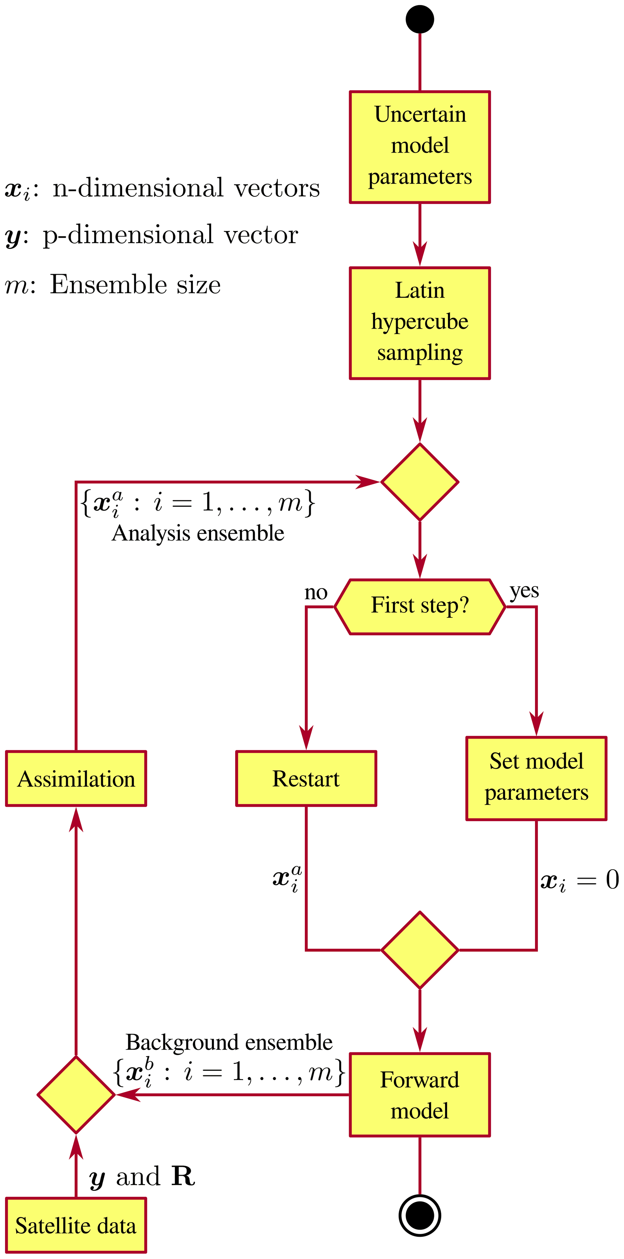
Figure 1Diagram of the modelling workflow used by FALL3D+PDAF when data assimilation (DA) is enabled. Assimilation is performed by means of an ensemble-based DA technique based on a sequential scheme.
For each assimilation cycle, the analysis step requires a background ensemble . The background states are produced by means of a forward model by evolving the ensemble of system states until a time with valid observations. At this point, a dataset of observations (including error observations) is incorporated to produce an ensemble of analyses . The corresponding analysis for each ensemble member is used as the model initial condition for the next cycle, and the forward model is restarted from the observation time. Finally, the assimilation cycle is repeated until the end of the simulation. It should be noted that model parameters are defined before simulation starts, and these parameters are not resampled during subsequent assimilation cycles.
In this work, the model state for each ensemble member is propagated by the FALL3D dispersal model. The DA system builds upon an efficient implementation by coupling FALL3D and the Parallel Data Assimilation Framework (PDAF), an open-source software environment for ensemble data assimilation providing fully implemented and optimised data assimilation algorithms, including ensemble Kalman filters (KFs) such as EnKF, ETKF, and LETKF (Nerger et al., 2005, 2020, see also Sect. 2). PDAF supports an efficient use of parallel computers and facilitates its implementation by combining an existing numerical model with a group of DA algorithms with minimal changes in the model code. We used the PDAF version 1.14 that, in addition to KF algorithms, also includes an ensemble square root filter for nonlinear data assimilation, referred to as the nonlinear ensemble transform filter (NETF; Tödter and Ahrens, 2015), and a particle filter (PF; e.g. Gordon et al., 1993).
The FALL3D+PDAF system can be run in parallel and supports online-coupled DA, enabling the workflow to be executed in a single step and with an efficient data transfer management through parallel communications. This avoids the creation of extremely large files that would be required to store the full system state in case of an offline approach. The implementation uses a two-level parallelisation scheme based on MPI (message passing interface) and can benefit from high-performance computing (HPC) resources. The two-level parallelisation scheme is sketched in Fig. 2. During the ensemble forecast phase, m instances of FALL3D, referred to as model tasks, are run concurrently as an embarrassingly (or perfectly) parallel workflow to evolve the member states in time (level 1). In other words, the problem is separated into a number of parallel tasks running independently that require no communication or dependency between ensemble members. In turn, each model task is executed by a single parallel instance of FALL3D, which uses a three-dimensional domain decomposition with nx, ny, and nz sub-domains along each direction (level 2). Consequently, the ensemble forecast requires a total of MPI processes. Multiple intra-member (level 1) communications are required during each assimilation step in order to collect and distribute the state vectors between different parallel tasks. Specifically, model tasks communicate with the master model task (i.e. the first model task in Fig. 2) during the analysis stage, and filter operations required to produce the analyses are performed exclusively by the MPI processes corresponding to the master model task.
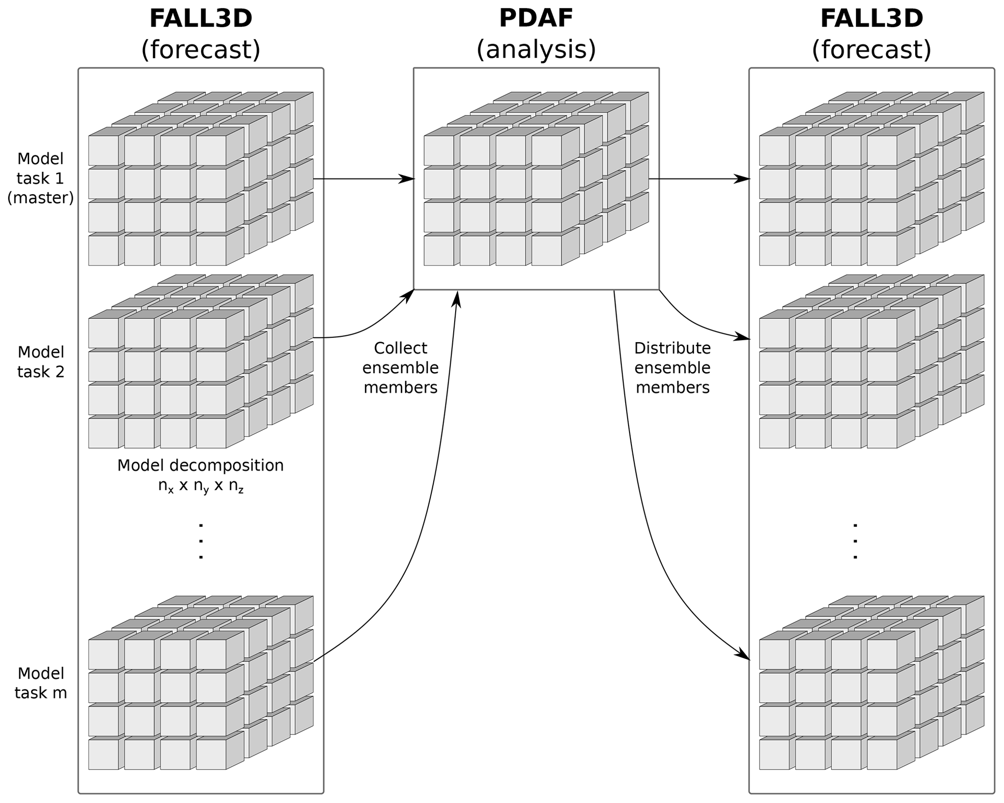
Figure 2Scheme of the ensemble-based data assimilation system implemented in the FALL3D dispersal model. The system builds upon an efficient implementation by coupling FALL3D and the Parallel Data Assimilation Framework (PDAF) and uses a two-level parallelisation scheme based on MPI (message passing interface).
3.2 Data assimilation setting
Two ensemble Kalman filter algorithms have been implemented in the FALL3D+PDAF system: ETKF and LETKF. As stated in Sect. 2, we will focus exclusively on the localised version of the ETKF proposed by Hunt et al. (2007), i.e. LETKF. Localisation in LETKF is performed by partitioning the state vector into a number of local domains defined by the vertical column corresponding to a single cell of the horizontal model grid and includes all bin species contributing to the observed column mass. Local analysis is performed by computing a separate analysis for each local domain and considering only observations within a volume defined by a cylinder of radius LR. No vertical localisation is used since observations are column integrated (see Sect. 3.4). A separate analysis is then generated for each model grid point in the local domain. By default, a uniform weight (unit weight) is assumed for all observations contributing to the local analysis. Alternatively, the influence of observations can also decay exponentially with the distance r from the analysis location according to a weight with the dependency , where the exponential decay radius, LSR, is a user-defined input.
Table 1 lists the parameters required by the FALL3D input file to configure the data assimilation system. In addition to start–end time and frequency of assimilation, local range (LR) and inflation factor (λ) can be defined in this block (see Sect. 2). Note that the covariance inflation factor is expressed here in terms of the so-called forgetting factor, defined as (Nerger et al., 2012). Other parameters include satellite filename, type of observation weighting, and cut-off diameter for volcanic ash (i.e. maximum particle diameter to compute mass loading). The parameter TRANSFORMATION specifies how the Λ matrix, defined in Appendix A by Eq. (A7), is computed conforming to two possible transformation options: identity matrix (DETERMINISTIC) or random rotation (RANDOM_ROTATION). As explained below in Sect. 3.3, the parameter SQRT_TRANSFORMATION allows the user to specify whether a nonlinear transformation should be applied to the model state variable.
Table 1List of input parameters required by the data assimilation block in the FALL3D input configuration file.
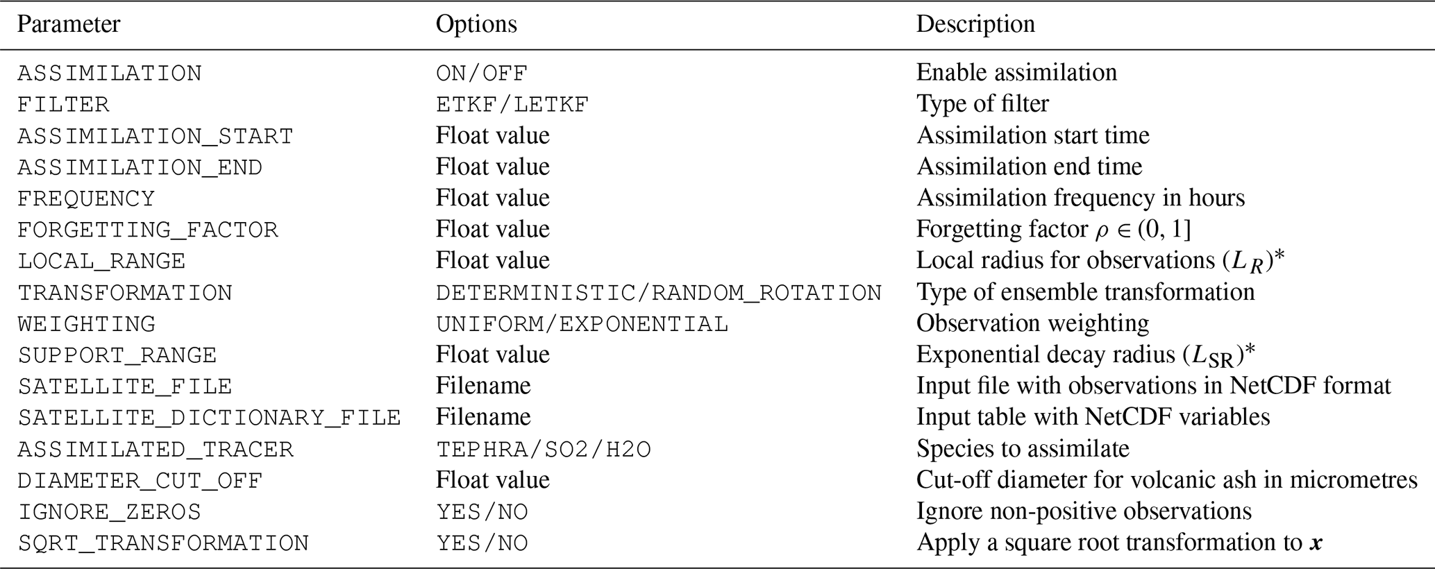
∗ LR and LSR are defined in units of the model grid size.
Alternative ensemble-based techniques provided by PDAF, such as PF and NETF (see Sect. 3.1), will be implemented in future releases of FALL3D. While the ensemble Kalman filters implicitly assume that the prior state and the observation errors are Gaussian, NETF and PF methods are not restricted by the assumptions of linearity or Gaussian noise. In contrast, PF and NETF are exposed to weight collapse due to the so-called curse of dimensionality (e.g. Carrassi et al., 2018). In addition, Kalman filters are expected to outperform NETF and PF in a linear and Gaussian problem (e.g. see Tödter and Ahrens, 2015). FALL3D solves an almost linear problem with weak non-linearity effects (e.g. due to gravity current, wet deposition, or aggregation). However, as discussed next, the Gaussian hypothesis is not fulfilled, leaving open the question of which is the best approach to deal with the assimilation of volcanic aerosols.
3.3 Model state
The DA algorithm requires a model state vector x∈ℝn, which is corrected in the analysis step. The state vector is constructed from the three-dimensional concentrations at the assimilation time t for the bin species i (). As concentration is a positive-semidefinite variable, the prior PDF associated with the ensemble forecast tends to show a right-skewed distribution. To illustrate this aspect, the two-dimensional histogram in Fig. 3a shows the skewness (i.e. , the third standardised moment) of the prior PDF computed for each grid cell at the first assimilation time for the Raikoke experiment (see Sect. 4.2). Note that a positive skewness () predominates in all points, with the most probable value () occurring when the mean-to-sigma ratio (i.e. , the mean-to-standard deviation ratio) approaches zero. Interestingly, the relationship (solid red line) defines a lower boundary which is satisfied for almost all points (). The skewness of the a priori PDF tends to the expected value for a normal distribution () only for large values of . However, values of above 0.5 are extremely unlikely to occur, and, in general, skewness values satisfy . This has important implications, as the Gaussian hypothesis assumed by the Kalman filter theory is not satisfied. As a result, the analysis step can yield an unrealistic posterior estimate, including negative concentrations.
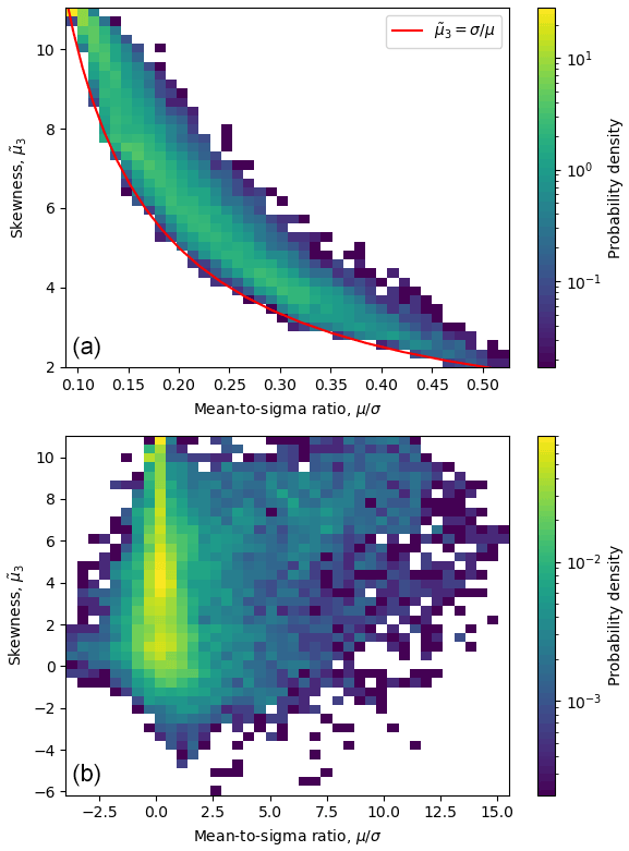
Figure 3Two-dimensional histogram plot for the prior (a) and analysis (b) distributions showing the probability density for skewness () and mean-to-sigma ratio () values, where μ refers to ensemble mean and σ to standard deviation. Results correspond to the first assimilation cycle of the Raikoke experiment.
This is illustrated in Fig. 3b, which shows the two-dimensional histogram plot for the posterior distributions resulting from the LETKF. Clearly, the statistics of the analysis ensemble tend to become Gaussian, and, as a result, the algorithm generates an unrealistic ensemble which is not consistent with the non-Gaussian Bayes' theorem, introducing artificial negative values for both ensemble mean and skewness.
In this work, we follow a simple approach to partially fix this problem by removing negative concentrations (a zero value is assigned). This truncated state is no longer a solution of the original Kalman filter problem, and the ability of this method to produce an improved state should be explicitly demonstrated. The probability of obtaining nonphysical solutions increases with the local radius for observations (LR) and with the number of observations close to zero. For these reasons, global filters such as ETKF are not considered here. On the other hand, only observations with positive column mass exceeding a given threshold, related to the detection limit of satellite sensors, are assimilated.
In addition to removing negative data, we also explored an alternative definition of the vector state x in terms of some nonlinear transformation x=T(C), so that background concentration values close to zero are stretched out. A logarithmic function or the square root are two obvious options for T. In this way, the filtering process occurs in the transformed space, and, after the analysis, concentration can be recovered by applying the inverse transformation, i.e. ). This “transformed state” approach failed with a logarithmic mapping due to the existence of few outliers leading to extremely large concentrations when the inverse transformation was applied. In contrast, the square root transformation resulted in reasonable results and a stable filter. In practice, the square root transformation can be enabled by the user through the FALL3D input parameter SQRT_TRANSFORMATION, as indicated in Table 1.
3.4 Observation operator
The DA system supports assimilation of satellite-retrieved mass loading (i.e. the vertical column mass per unit area) of volcanic ash and gases (SO2 and H2O). As a consequence, the objective is to reconstruct the three-dimensional concentration field of each species i from a two-dimensional observational dataset. The observation operator H, which projects a model state x∈ℝn onto the observation space, entails a vertical integration of concentration, a sum over different species (if multi-species observations are being assimilated), and, finally, the interpolation to the observation coordinates. Note that, if the vector state x represents mass concentration, H is a linear operator. This is the main advantage of focusing on mass loading rather than on other observable physical quantities, e.g. aerosol optical depth, which would lead to a nonlinear observation operator.
The observation operator acting over the analysis vector defines a vector ya∈ℝp of analysed mass loading:
where is the assimilated state vector (analysis).
In order to facilitate the visualisation and enable a direct comparison with observations, the analysed mass loading, ya, will be shown in the following figures. However, if not explicitly stated otherwise, the full analysis state, i.e. , will be used to compute the evaluation metrics (see Sect. 3.7).
3.5 Ensemble generation
In order to generate a set of m background states, FALL3D automatically perturbs eruption source parameters (ESPs) and horizontal wind components from a reference value using either uniform or truncated normal distributions (Folch et al., 2021). A Latin hypercube sampling (LHS; McKay et al., 1979) is used to efficiently sample the parameter space. Table 2 lists the perturbed parameters in the twin and Raikoke DA experiments that are considered in this work (see Sect. 4).
Table 2Ensemble configuration for the twin and Raikoke experiments. In order to generate the ensemble, eruption source parameters (ESPs) and wind components were perturbed around a reference value using either uniform or truncated normal distributions. The Latin hypercube sampling (LSH) method is used to sample the parameter space. The perturbed ESPs are eruption start time (Ti), source duration (ΔT), eruption column height (H), mass emission rate (MER), parameters As and λs of the Suzuki vertical mass distribution, and top-hat thickness (ΔZ).
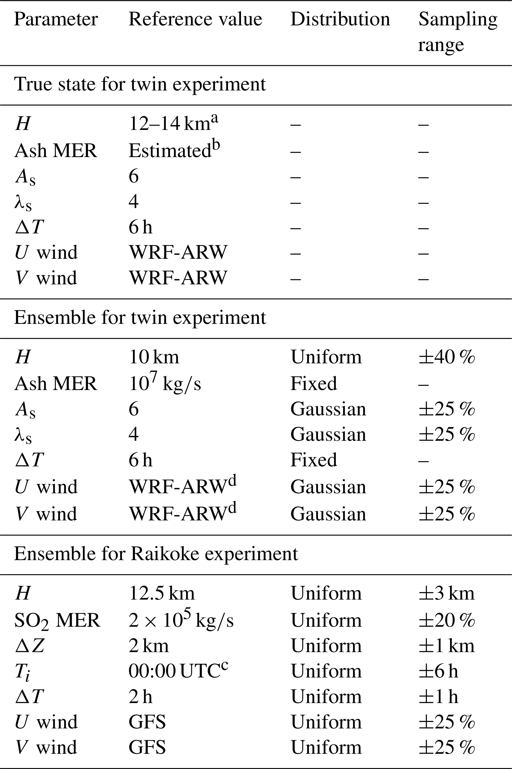
a Variable column height as in Fig. 4. b Parameterisation from Degruyter and Bonadonna (2012). c On 22 June 2019. d Weather Research and Forecasting-Advanced Research WRF.
3.6 Satellite retrievals
The satellite retrievals used for the Raikoke DA experiment are SO2 mass loading retrievals derived from AHI/Himawari-8 measurements. Details of the retrieval method are described in Appendix B of Prata et al. (2021). The retrieval is based on the strong absorption of SO2 near the 7.3 µm wavelength and is generally only sensitive to upper-level (≳ 4 km) SO2 due to the masking effect of water vapour absorption at lower levels in the atmosphere (Prata et al., 2004). A conservative estimate of the relative uncertainty on these mass loading retrievals is 30 %.
3.7 Evaluation metrics
When the true state xtr∈ℝn is known (e.g. experiments with synthetic observations as in Sect. 4.1), the difference between the ensemble mean and the truth can be directly quantified using the average root-mean-square error:
In contrast, for the case involving real observations (see Sect. 4.2), the root-mean-square error is computed in the observation space according to
where y∈ℝp represents a vector with p observations, and ya is the analysed mass loading vector defined by Eq. (6).
A measure of the uncertainty of the ensemble is given by the ensemble spread, σe. The domain-averaged spread can be defined in terms of the ensemble-based covariance matrix as
where Pe is the ensemble-based matrix for the covariance defined by Eq. (2), and tr(Pe) denotes the trace of Pe. Note that the true state is not involved in this definition, meaning that this metric is independent of xtr.
Additionally, we also consider categorical metrics defined for model and observations from the exceedance (or not) of a given threshold. For example, in the case of categorical metrics for the total column mass loading, a true positive means that both model and observation exceed a given threshold value. The true positive rate or probability of detection (POD) is defined as the number of true positives (n+) divided by the number of false negatives (n−) plus the number of true positives (n+):
The POD ranges from 0 to 1 (optimal), and, geometrically, it can be interpreted as the area of the intersection between the modelled and observed column mass contours, normalised by the area of the observation contour (Folch et al., 2021).
This section presents results from two numerical experiments aiming at evaluating the performance of the FALL3D+PDAF DA system under different filter configurations. The first experiment (twin experiment) is described in Sect. 4.1, and the second experiment (Raikoke experiment) is described in Sect. 4.2. Table 3 summarises the model configuration defined for each experiment.
Table 3Model configuration parameters for the numerical experiments considered in this work.
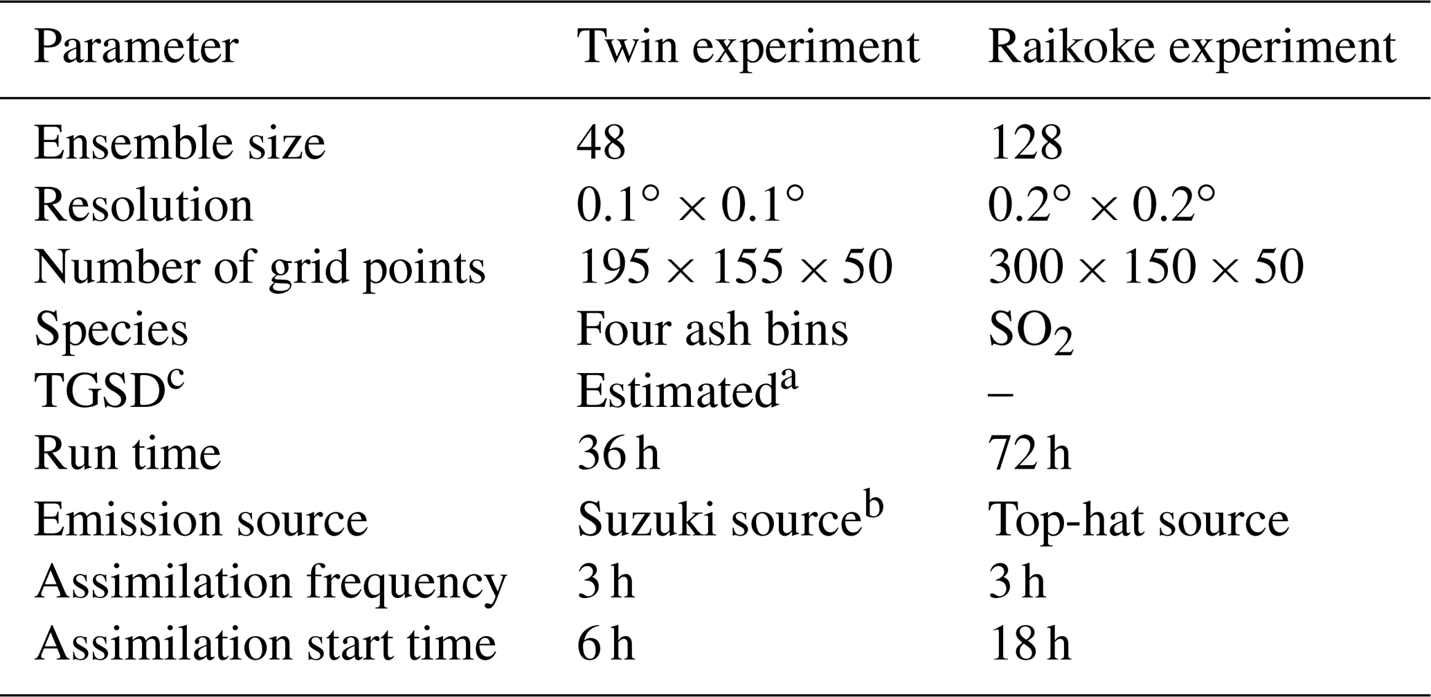
a Costa et al. (2016a). b Pfeiffer et al. (2005). c Total grain size distribution.
A critical aspect in operational workflows is the computational cost required by the ensemble forecasting system. FALL3D has been proven to have a good strong scalability (above 90 % of parallel efficiency) up to several thousands of processors (Folch et al., 2020). As the ensemble forecasting task is embarrassingly parallel, major constraints on computing time probably come from the analysis step. Simulations were conducted on the Joliot-Curie supercomputer at the CEA's Very Large Computing Center (TGCC, France) using 1152 processors for the twin experiment (ensemble size: 48) and 3072 processors for the Raikoke experiment (ensemble size: 128). The typical computing times were of around 200 s (twin experiment) and 375 s (Raikoke experiment).
4.1 Twin experiment
Twin experiments are commonly used to evaluate DA methods. In this case, the truth state is generated by a model run in order to obtain a reference vector state. Synthetic observations are generated by adding random perturbations, which represent non-correlated observation errors, to the true state. An ensemble forecast is then produced by perturbing a state estimate (different from the truth), and synthetic observations are assimilated. The performance of the ensemble filter can be evaluated by comparing the assimilation results with the true state.
The twin case study considers a fictitious eruption from Etna driven by WRF-ARW meteorological data in order to produce realistic atmospheric conditions. As stated in Table 3, a 36 h numerical simulation was performed considering an eruption lasting 6 h with a mass emission rate (MER) estimated from the eruptive column height (H) according to Degruyter and Bonadonna (2012). The (synthetic) time evolution of column height is shown in Fig. 4.
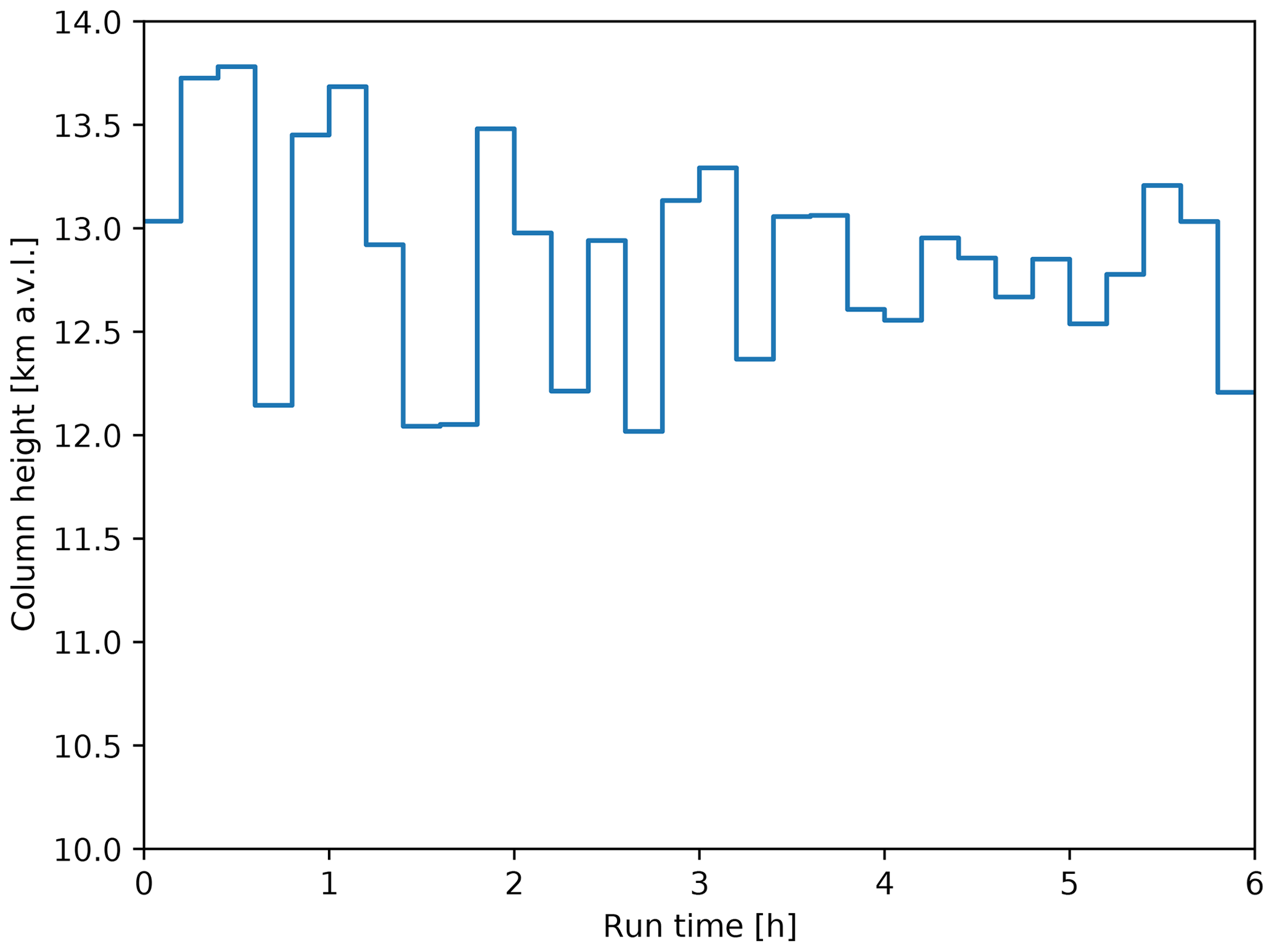
Figure 4Time evolution of the eruption column height used to define the twin experiment true state. The 6 h duration eruption is characterised by multiple eruptive phases with a duration of 20 min and column height randomly sampled within the range 12–14 km above the vent.
In a previous study including several cases, Costa et al. (2016b) found a maximum column height variability of 30 % for weak plumes and 10 % for strong plumes. Moreover, Suzuki et al. (2016a, b) showed that a variability of up to ∼ 20 % can simply be due to internal plume dynamics. Correspondingly, the twin experiment in this work considers multiple eruptive phases with a duration of 20 min and a column height sampled from a uniform probability distribution within the range 12–14 km above the vent (15.3–17.3 km a.s.l.). Such a time-varying source term can result in complex cloud dynamics and represents a challenge for dispersion models and DA. The Suzuki plume option was adopted for the vertical distribution of mass (Pfeiffer et al., 2005), and the total grain size distribution was estimated from the time-varying column height following the parameterisation proposed by Costa et al. (2016a) assuming a magma viscosity of η=105 Pa s. The computational domain has a horizontal resolution of 0.1∘ and a domain size of grid cells. Simulations involve four fine ash bins (nb=4) with particle diameters d<10 µm, and, consequently, the dimension of the state vector x used in the assimilation cycle is .
Synthetic observations were generated by adding a Gaussian noise to the column mass loading computed from the true state. As in Pardini et al. (2020), a conservative relative error of 40 % is considered for both the synthetic observations and the Raikoke SO2 retrievals. In order to represent a realistic scenario where the range of valid measurements is restricted by the instrumental detection limit, we assume mass loading observations are above a given threshold. For example, Prata and Prata (2012) suggested a detection limit of 0.2 g m−2, approximately, for SEVIRI retrievals of ash mass loading. On the other hand, Mingari et al. (2020) found a good correlation between MODIS airborne ash detection products and the 0.1 g m−2 mass loading contours simulated by FALL3D. In this work, synthetic observations were defined assuming a mass loading threshold of 0.15 g m−2.
The twin experiment considers a 48-member ensemble and two types of simulations: (i) a free run without assimilation and (ii) a set of LETKF runs, where observations were incorporated with an assimilation frequency of 3 h beginning at t=6 h after the simulation start (the total simulation time was 36 h). To generate the ensemble, the column height was uniformly sampled around a reference value of 10 km with a perturbation range of 40 % and assuming a fixed mass flow rate of 107 kg s−1 (see Table 2). Since both eruption column height and eruption rate are assumed to be constant here, no single member can actually reproduce the true state by itself because the control run was defined from a time-varying source term (Fig. 4). Furthermore, the ensemble central column height (H=10 km) tends to underestimate the true column height. Consequently, the ensemble was not optimally constructed to mimic a realistic situation in an operational forecasting workflow in which the exact column height is unknown.
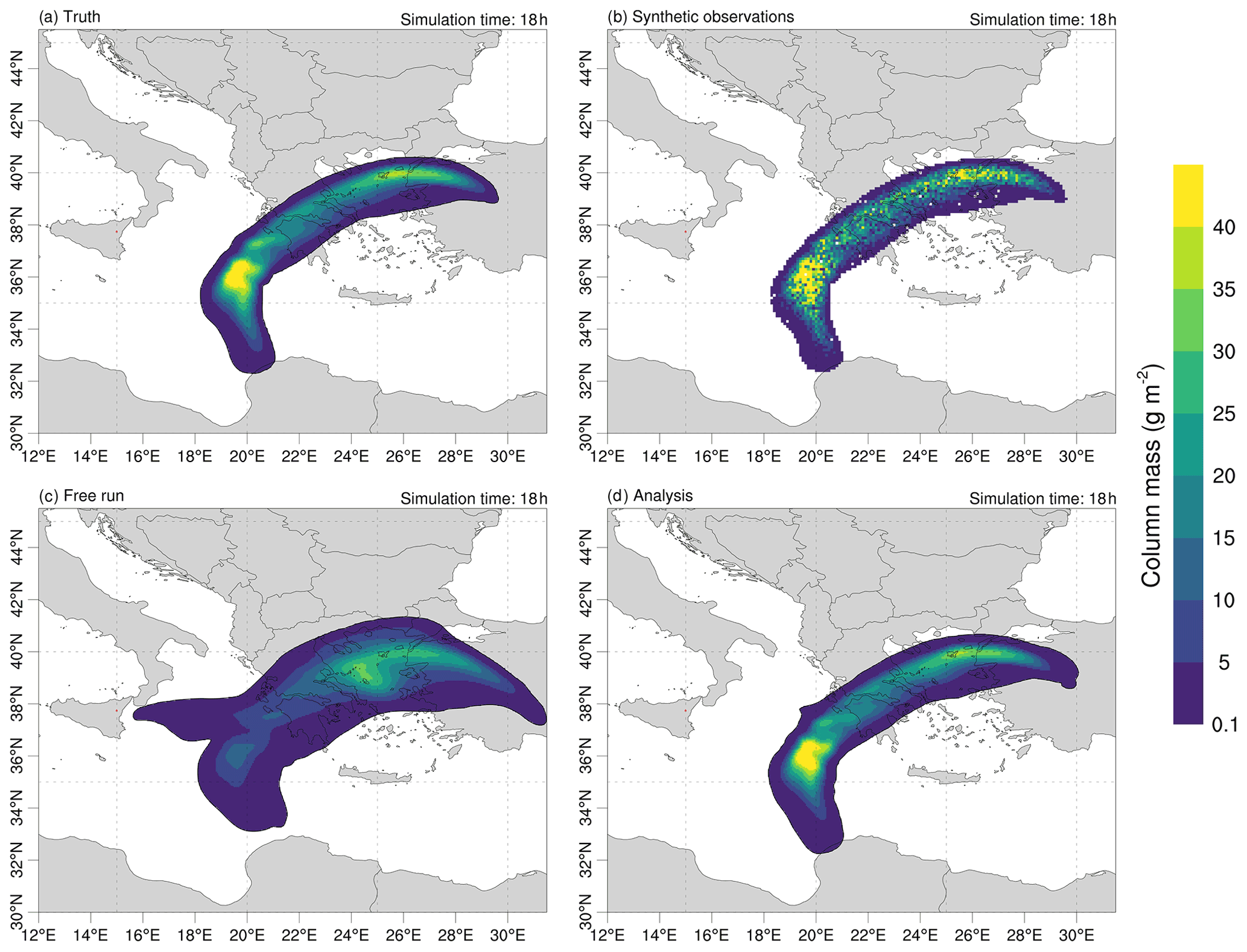
Figure 5Spatial distribution of ash mass loading for the twin experiment at t=18 h after eruption start. The true state (a) given by a single run assumes a time-varying emission. Synthetic observations (b) are generated from the truth by adding a Gaussian noise and assuming an observation error variance of 40 %. The impact of the LETKF DA becomes evident by comparing results from the free ensemble run without assimilation (c) with the analysed mass loading (d).
4.1.1 Twin experiment results
The spatial distribution of mass loading is shown in Fig. 5 at simulation time t=18 h after the eruption start time according to the true state (Fig. 5a), synthetic observations (Fig. 5b), ensemble free run without assimilation (Fig. 5c), and LETKF analysis (Fig. 5d). In all cases, the ash cloud for this idealised eruption is transported eastwards by upper-level winds. As expected, the free run case shows a broader spatial distribution than the true state due to the ensemble spread. Moreover, the free run incorrectly predicts the location of the column mass maximum occurring over the northern region of the cloud. In contrast, the analysed mass loading field approaches the true state after a few assimilation cycles (Fig. 5d).
To quantify the impact of DA, the RMSE and ensemble spread were computed using Eqs. (7) and (9). Figure 6a shows the time-averaged (over the whole simulated period) RMSE for different localisation radii and two multiplicative inflation factors of λ=1 (black triangles) and λ=1.2 (red circles). Simulations were repeated three times to inspect the impact of the random noise, and the resulting metrics were averaged (solid lines). Despite the large scattered data, optimal localisation radius seems to be between and (20 to 40 grid cells), with a notorious degradation of performance for (see Fig. 6a). Increasing the inflation factor from λ=1.0 to λ=1.2 resulted in slightly smaller RMSE in most of the ensemble realisations (Fig. 6a).
Hourly time series of the evaluation metrics are shown in Fig. 6b for the free and LETKF runs (analysis times are indicated by star symbols). The optimal parameters and λ=1.2 were used here to configure the LETKF run. As expected for a diffusive process without sources, the RMSE decreases from t=6 h, when the eruption ends. Clearly, the LETKF simulation outperforms the free run. The impact of DA becomes more apparent by looking at the relative RMSE, i.e. the LETKF-to-free ratio of RMSE. In the first assimilation cycle at t=6 h, the relative RMSE decreases abruptly from 1 down to ∼0.2. During successive assimilation cycles this ratio decreases further, suggesting that the analysis is converging to the true state.
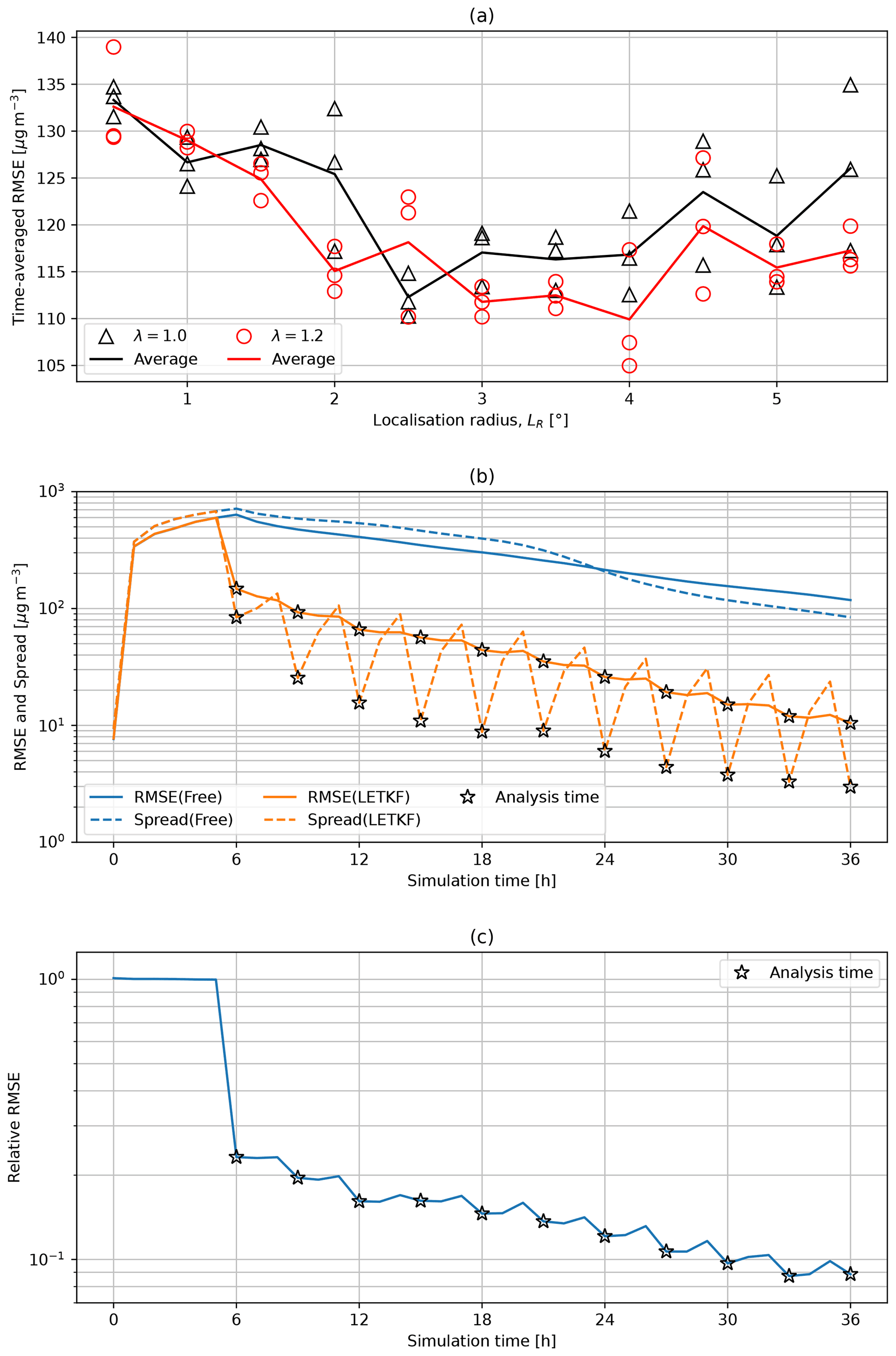
Figure 6Evaluation metrics used for the twin experiment are as follows. (a) Time-averaged RMSE computed for different filter configurations and three ensemble realisations. Best performance was obtained for localisation radius, LR, in the range 2–4∘and an inflation factor of λ=1.2. (b) Temporal evolution of ensemble spread and RMSE for the free and LETKF runs. (c) Time series of LETKF-to-free ratio of RMSE. Assimilation times are denoted by star symbols.
The ensemble spread should be close to the analysis error since under-dispersive ensembles are prone to filter divergence. As depicted in Fig. 6b, a steep decrease in spread occurs at each assimilation time, which is compensated for by the ensemble variability introduced during each forecast period. The 3 h assimilation frequency turned out to be sufficient to keep spread just above the RMSE during each assimilation cycle, meaning that uncertainties are correctly represented by the ensemble.
In conclusion, the twin experiment shows that it is possible to reconstruct the original 3D model state of concentration field from an incomplete dataset of 2D measurements subject to uncertainty. A good filter performance was achieved despite the fact that column mass data below 0.15 g m−2 were discarded, i.e. the fact that only a fraction of the available column mass data were actually assimilated.
4.2 The 2019 Raikoke eruption
On 21 June 2019, the Raikoke volcano (48.292∘ N, 153.25∘ E) in the Kuril Islands (Russia) had a significant eruption that disrupted major flight routes across the North Pacific (Prata et al., 2021). The eruption injected ash and gases into the atmosphere in a sequence of around 10 eruptive pulses, from the initial explosive phase at 18:00 UTC on 21 June until 10:00 UTC on 22 June (Muser et al., 2020). The eruption sequence was captured by the Himawari-8 satellite at both IR and visible wavelengths. A remarkable amount of SO2 was injected into the atmosphere during these explosive phases, producing a long-range transport of SO2 that could be detected by satellite instrumentation.
In order to simulate this event, the FALL3D computational domain was configured using a horizontal resolution of 0.2∘ and a domain size of grid cells. In this case, the state vector x includes only SO2 and has a size of . For this experiment, 72 h numerical simulations were conducted starting on 21 June 2019 at 18:00 UTC using 128 ensemble members. A free run without DA and several LETKF runs were performed for comparative purposes. Assimilation starts on 22 June 2019 at 12:00 UTC with a frequency of 3 h for the successive assimilation cycles. The top-hat option was adopted for the vertical mass distribution in the source term; i.e. the source term is defined by a uniform mass distribution along a layer of thickness ΔZ and top at height H. Both parameters were perturbed with central values of ΔZ=2 km and H=12.5 km above sea level. In addition, mass emission rate (MER), start time and duration of eruption, and wind components were also perturbed. Specifically, the emission start time was uniformly sampled between 18:00 UTC on 21 June and 06:00 UTC on 22 June, assuming a duration of h for each ensemble member. Note that the eruption total time for Raikoke was around 14 h, meaning that each ensemble member represents a possible eruptive phase lasting a fraction of the total eruption time. This approach was adopted in order to reproduce a multi-phase eruptive scenario with a complex time-varying emission source term. In this case, the real state involves a mixture of multiple ensemble members with weights to be determined by the analysis step.
The list of model parameters used to generate the ensemble is detailed in Table 2, and Table 3 summarises the general model configuration used in the Raikoke experiment. The dispersal model was driven by meteorological data from the Global Forecast System (GFS) model instead of using reanalysis data in order to replicate an operational forecasting environment.
4.2.1 Raikoke experiment results
Figure 7 compares the spatial distribution of SO2 mass loading according to the satellite retrievals (left panel), free run (central panel), and analysis (right panel) at three time instants. On 22 June, the volcanic plume is influenced by upper-level zonal winds and moves eastwards crossing the 180th meridian. From 23 June, the plume of sulfur dioxide gets trapped within the cyclonic circulation of the Aleutian low, causing the airborne material to spiral anticlockwise for several days (Kloss et al., 2021).
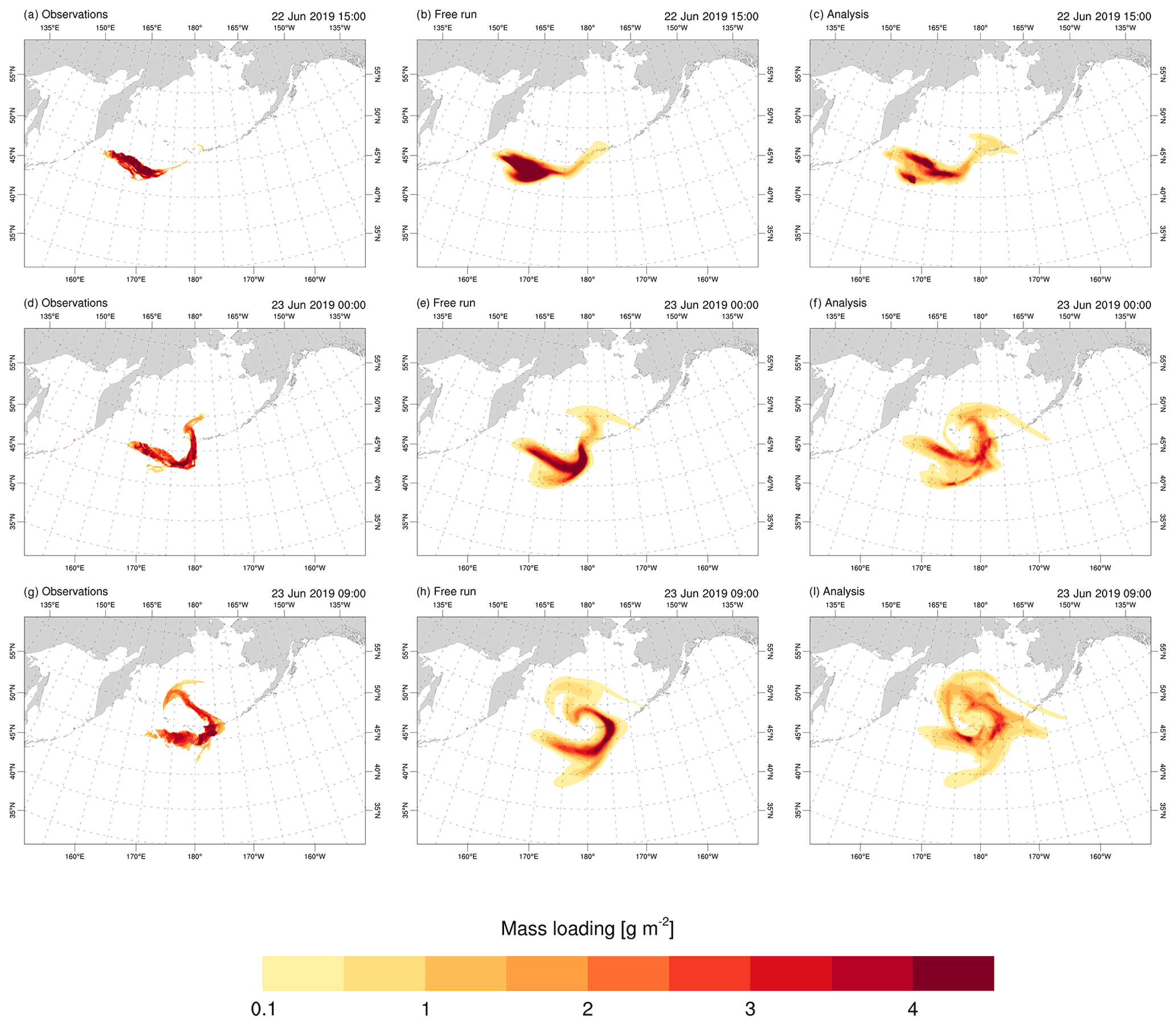
Figure 7Spatial distribution of SO2 mass loading at different time instants: (a–c) 22 June at 15:00 UTC, (d–f) 23 June at 00:00 UTC and (g–i) 23 June at 09:00 UTC. The column panels show observations (left panel), free run (central panel) and analysed mass loading (right panel). Panels in the central and right columns correspond to ensemble means.
In order to assess the filter performance, two quantitative metrics defined in Sect. 3.7 will be considered below. First, the root-mean-square error (RMSEo) is computed in the observation space using Eq. (8). Figure 8a shows the RMSEo for all the analysis states using different localisation radius (LR=2, 4 and 6∘). Despite the occurrence of nonphysical solutions (grid cells with negative concentrations) during the first assimilation cycle, the truncated LETKF solutions outperform the free run in all cases. After successive assimilation cycles, the ensemble analysis becomes closer to a Gaussian distribution, and the probability of obtaining nonphysical solutions diminishes. Results in Fig. 8 also show that RMSEo decreases with the localisation radius. Specifically, the time-averaged RMSEo (Fig. 8b) decreased from 1.08 g m−2 () to 0.87 g m−2 (). Overall, the analysis errors were decreased by more than 50 % relative to the free run errors. However, it is important to highlight that it is not possible to infer the filter performance was improved by decreasing the localisation radius as no true state is now available to compute the actual RMSE (see Sect. 4.1). Finally, Fig. 8b also shows results for the LETKF (sqrt) simulations, where the option SQRT_TRANSFORMATION was enabled (see Sect. 3.3), meaning the vector state was constructed from the square root of the concentration. This approach resulted in a slightly smaller RMSEo, but the impact does not appear to be significant.
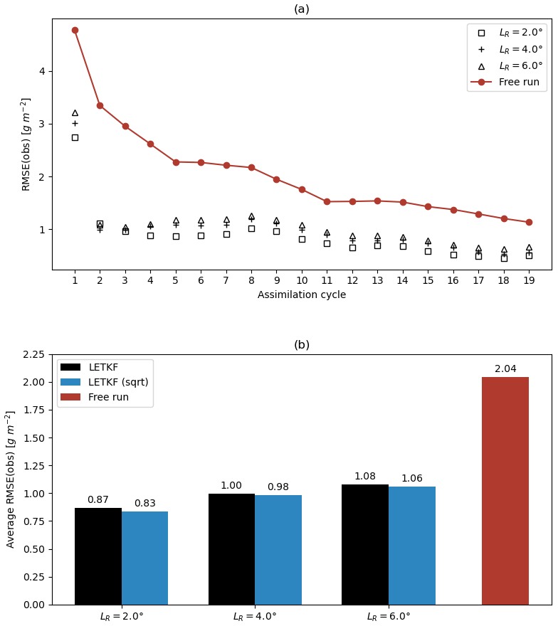
Figure 8RMSEo computed in the observation space for the Raikoke experiment: (a) time series of RMSEo at analysis times for the free (red line) and LETKF runs for different localisation radii (, and ) and (b) the same with time-averaged values.
While the free run results show a very poor correlation between observed and modelled SO2 mass loading, a clear correlation emerges after a few assimilation cycles in the LETKF simulations. As an example, Fig. 9 shows a comparison between the observed and analysed mass loading at the fourth assimilation cycle. A systematic bias, likely caused by the characteristics of the ensemble distribution, was found at each assimilation cycle, and analysis tends to underestimate observations. In this particular cycle, for instance, an average bias of 0.41 g m−2 was found.
The spatial distribution of observed and analysed mass loading for the SO2 cloud on 23 June at 12:00 UTC is shown in Fig. 10 along with the cloud top height derived from the analysed state. A complete sequence of the temporal evolution for this figure can be found in the Supplement. The cloud top height is defined as the upper height of a given iso-concentration contour (50 µg m−3 was assumed here). The model can correctly capture the position of the SO2 plume for mass loading contours above 1 g m−2. However, no observations are available below 0.5 g m−2 (e.g. see Fig. 9), making the comparison for low mass loading values challenging. Specifically, the analysed mass loading indicates the existence of a low-level cloud in the southern region that could not be detected by the satellite retrievals.
Finally, we computed categorical metrics based on the 1 g m−2 contour of SO2 mass loading. The resulting maps are shown in Fig. 11 for three time instants. The complete time sequence can be found in the Supplement. The plume dynamics according to the free run (top panel) follows a similar pattern to that found in previous simulations by Prata et al. (2021). Specifically, the free run (solid red line) and observed contours (green shaded area) diverge after a few time steps. In contrast, the contours corresponding to simulations with data assimilation evolve concurrently with observations for all simulated times (Fig. 11, bottom panel).

Figure 9Comparison of SO2 mass loading observations and the analysis state at the fourth assimilation cycle. In general, analysis underestimates observations. In this case, an average bias of 0.41 g m−2 was found.
The performance of the simulations can be quantified through the POD categorical metric (Eq. 10), which can be interpreted geometrically as the ratio between the intersection area delimited by both the observation and model contours and the total area of the observation contour. Figure 12 shows the temporal evolution of the POD. After a forecast time of around t=18 h, this metrics tends to decrease monotonically for the free run, whereas it remains close to the optimal value (POD = 1) along all time steps when data assimilation is enabled. A sudden increase in this metric occurs at each assimilation cycle (square symbols), clearly visible from Fig. 12, which prevents this metric from degrading significantly. In conclusion, POD remains in the range around 0.8–0.9.
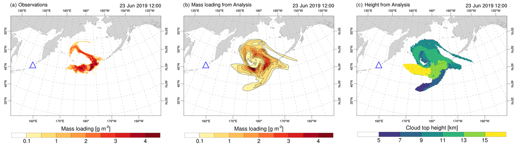
Figure 10SO2 cloud for the 2019 Raikoke eruption on 23 June at 12:00 UTC. Observed (a) and modelled (b) mass loadings are compared at the same instant of time. In addition, the cloud top height (c) derived from the analysed state is also shown. The LETKF run was configured assuming a localisation radius of and an assimilation frequency of 3 h, starting on 22 June 2019 at 12:00 UTC.

Figure 11Maps of 1 g m−2 contour of SO2 mass loading according to observations (green shaded area) and model (solid red line) for different instants of time: (a) 00:00 UTC on 23 June 2019, (b) 18:00 UTC on 23 June 2019 and (c) 12:00 UTC on 24 June 2019. Model results corresponding to the free run (top panel) and the analysis (bottom panel) are compared. A localisation radius of was defined for the data assimilation method.
In this work, a localised version of the ensemble Kalman filter LETKF has shown to be a promising alternative for assimilation of volcanic aerosols. Despite the limitations of this method, resulting in suboptimal filter performance, our findings do nevertheless show that a significant improvement of evaluation metrics was achieved.
Ensemble Kalman filters give an optimal state estimate under the following implicit assumptions: (i) the distribution of the background is Gaussian, (ii) the observational error has Gaussian distribution, and (iii) the forward model and observation operator are linear. FALL3D is a dispersal model with weak nonlinear terms, and modelling complex multi-phase eruptions entails the contribution of multiple ensemble members to properly represent the model state. However, in this work it has been shown that skewness is a significant issue, and the condition (i) is largely violated, resulting in suboptimal behaviour from the EnKF.
Different approaches have been proposed for dealing with non-Gaussianity, including variable transformations (e.g. Zhou et al., 2011; Amezcua and Van Leeuwen, 2014) and Bayesian approaches, such as a particle filter (e.g. van Leeuwen and Ades, 2013) or the nonlinear ensemble transform filter (NETF; Tödter and Ahrens, 2015). Unfortunately, these methods suffer from a series of pitfalls. For instance, variable transformation applied to skewed prior distributions would require highly nonlinear transformations to obtain state variables fulfilling the Gaussianity conditions, again leading to suboptimal states. On the other hand, particle filters and NETF are exposed to weight collapse due to the so-called curse of dimensionality, which would result in a poor performance in complex eruptive scenarios with stochastic time-varying emission source parameters. In addition, although the aforementioned methods may be suitable for problems involving highly nonlinear processes, ensemble-based Kalman filters are expected to work better for linear and Gaussian problems (e.g. Tödter and Ahrens, 2015). In consequence, it is not clear which of these methods would result in a better performance for linear (or weakly nonlinear) and non-Gaussian problems.
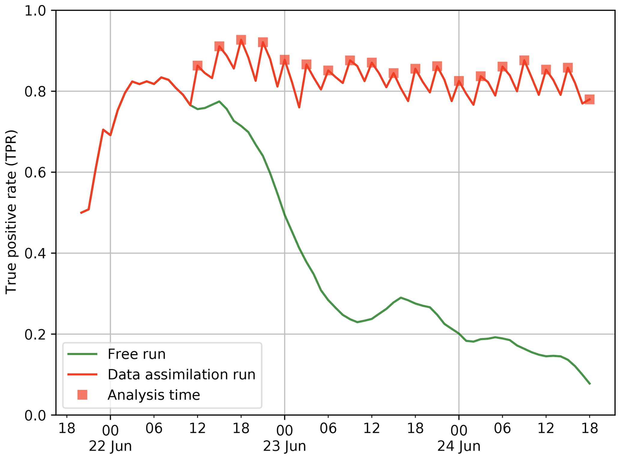
Figure 12Temporal evolution of the probability of detection (POD) metrics according to the free and data assimilation runs for the Raikoke experiment. A localisation radius of was defined for the data assimilation simulation.
Promising results obtained in this work using LETKF suggest that the natural approach for dealing with assimilation of volcanic aerosols in future research should focus on ensemble Kalman filters in which the Gaussian assumption is not made at all. For example, Bishop (2016) proposed an ensemble Kalman filter for highly skewed non-negative uncertainty distributions. This approach allows the EnKF to be generalised with few coding changes and little additional computational expense. Finally, higher-order EnKFs have also been proposed (e.g. Hodyss, 2012; Hodyss and Campbell, 2013) and could potentially address the aforementioned issues.
A detailed study has been conducted in order to assess the feasibility of using ensemble-based Kalman filters for data assimilation (DA) of volcanic aerosol observations. To this purpose, a new DA system based on coupling the FALL3D dispersal model with the Parallel Data Assimilation Framework (PDAF) has been implemented in the latest release of FALL3D (v8.2). The system supports online-coupled DA, can be run in parallel exploiting high-performance computing (HPC) resources and is suitable for an operational workflow. The computing time required by the numerical simulations carried out in this work ranges between 2 (twin experiment) and 6 (Raikoke experiment) minutes.
One of the major assumptions in the (ensemble) Kalman filters is that the prior model errors and the observation noise are Gaussian. However, ensemble forecasts of volcanic aerosols yield to a non-Gaussian prior, with positively skewed distributions. Consequently, the ability of the assimilation technique to produce an improved model state compatible with the available observations requires explicit verification.
We carried out two numerical experiments in which mass loading data were assimilated using the local ensemble transform Kalman filter (LETKF). Both test cases are characterised by complex plume dynamics and time-varying eruptive source parameters (ESPs) that pose a challenge to dispersion models, especially in operational environments. The complexities involved in the definition of the source term were intentionally discarded in the prior ensemble construction in order to replicate an operational environment, where such variations are typically unknown. A constant eruption column height (H) and mass emission rate (MER) were assumed for each ensemble member, meaning that no member can individually reproduce the case study correctly. In the twin experiment, the analysis converged to the true state when observations were continuously assimilated with a frequency of 3 h. In the second experiment, involving the SO2 plume produced by the 2019 Raikoke eruption, categorical metrics (POD) also remain close to optimal values as long as observations are continuously assimilated every 3 h.
Even though the results presented here are encouraging, the proposed truncated LETKF methodology is not optimal and should be tested in broader contexts and under different scenarios. We also encourage the community to test and develop more appropriate methodologies for positively skewed, non-Gaussian prior distributions.
The Kalman filter (KF) is a sequential data assimilation (DA) method that provides an optimal solution for linear models with linear observation operators (Kalman, 1960). In addition, KF also assumes Gaussian distributions for model errors and observation noise. If the state of a physical system can be represented by an n-dimensional vector, the analysis step of the KF consists in determining the a posteriori (analysis) state estimate, represented by a vector xa∈ℝn, and its associated covariance matrix , given a vector of observations y∈ℝp and the a priori (background) state estimate xb along with the error covariance matrix Pb. In the analysis step, the state estimate and covariance are updated according to the KF equations:
where is the observation operator that translates a model state x into the observation space and is the so-called Kalman gain matrix given by
where is the observation error covariance matrix. Note that any reference to time indices is omitted here. The Kalman gain matrix assigns relative weights to observations. A high-gain filtering implies more weight to measurements, whereas a low-gain filtering tends to follow the model more closely.
The ensemble Kalman filter (EnKF) is a family of methods in which the state estimate of the system is represented by an ensemble of system states that actually provide a Monte Carlo approximation of the KF and replace the original covariance matrix by a sample covariance matrix Pe computed from the ensemble (Evensen, 1994). Given an ensemble of background states , the analysis step consists in determining an ensemble of analyses in agreement with Eq. (A1a, b) but formulated in terms of the ensemble-based mean vector (Eq. 1) and covariance matrix (Eq. 2). The ensemble mean is updated using the standard KF analysis equation, Eq. (A1a),
with Ke being the ensemble-based Kalman gain matrix:
where we have defined Y=HXb and Xb is given by Eq. (3). Note that, with respect to Eq. (A2), the ensemble-based gain matrix Ke considers the ensemble background perturbations Xb and their projections onto the observation space through the matrix . In this way, the best estimate of the current state is determined in the analysis step through a weighted linear combination of the prior ensemble perturbations.
Different EnFK methods vary depending on how the ensemble analysis is defined so that the update for the ensemble covariance matrix is consistent with the original KF Eq. (A1a, b). Most formulations can be divided into two major categories, the stochastic (e.g. the perturbed observation-based EnKF formulation from Burgers et al., 1998) and the deterministic (Houtekamer and Zhang, 2016) approaches. The latter group includes the so-called square-root filters that use deterministic algorithms to generate the analysis ensemble (Nerger et al., 2012).
The ensemble transform Kalman filter (ETKF; Bishop et al., 2001) is a popular square-root filter formulation that is considered in this work. A square-root filter requires a matrix to transform the ensemble perturbations according to
In order to obtain the ensemble perturbations, the covariance update is required to be consistent with the original KF formulation given by Eq. (A1a, b), leading to (e.g. see Carrassi et al., 2018)
where is the so-called transform matrix, defined by (Nerger et al., 2012). If the square root is denoted by C (i.e. CC⊺=A), the weight matrix W is assumed to be expressed as
where is any orthogonal matrix preserving the ensemble mean (see Sect. 3.1). In this work, the symmetric square root is used to define C according to the symmetric factorisation
using the singular value decomposition: . This definition of the root square matrix ensures that the ensemble mean is preserved (Hunt et al., 2007).
FALL3D-8.2 is available under version 3 of the GNU General Public License (GPL) at https://gitlab.com/fall3d-distribution/v8 (last access: 12 January 2022). The PDAF code (version 1.14 was used here) and full documentation are available at http://pdaf.awi.de (last access: 11 November 2020) (Nerger et al., 2005, 2020).
The supplement related to this article is available online at: https://doi.org/10.5194/acp-22-1773-2022-supplement.
LM designed the research, analysed the data, prepared the figures, and wrote the draft. Simulations were performed by LM. The FALL3D model was developed by AF, AC, GM, and LM. ATP contributed to the Himawari-8 satellite retrievals. FP provided insightful comments about the assimilation technique and the PDAF library. LM wrote the final version of the article with contributions from AF, AC, and ATP. All authors have revised and approved the final version of the paper.
The contact author has declared that neither they nor their co-authors have any competing interests.
Publisher’s note: Copernicus Publications remains neutral with regard to jurisdictional claims in published maps and institutional affiliations.
This article is part of the special issue “Satellite observations, in situ measurements and model simulations of the 2019 Raikoke eruption (ACP/AMT/GMD inter-journal SI)”. It is not associated with a conference.
We acknowledge the Partnership for Advanced Computing in Europe (PRACE) for awarding us access to the Joliot-Curie supercomputer at the CEA’s Very Large Computing Center (TGCC, France). Andrew T. Prata acknowledges funding from the European Commission, H2020 Marie Skłodowska-Curie Actions (STARS (grant no. 754433)). We thank the anonymous reviewers for their insightful comments and suggestions.
This research has been partially funded by the H2020 Center of Excellence for Exascale in Solid Earth (ChEESE) under the grant agreement no. 823844.
This paper was edited by Farahnaz Khosrawi and reviewed by two anonymous referees.
Amezcua, J. and Van Leeuwen, P. J.: Gaussian anamorphosis in the analysis step of the EnKF: a joint state-variable/observation approach, Tellus A, 66, 23493, https://doi.org/10.3402/tellusa.v66.23493, 2014. a
Anderson, J., Hoar, T., Raeder, K., Liu, H., Collins, N., Torn, R., and Avellano, A.: The data assimilation research testbed: A community facility, B. Am. Meteorol. Soc., 90, 1283–1296, 2009. a
Anderson, J. L. and Anderson, S. L.: A Monte Carlo Implementation of the Nonlinear Filtering Problem to Produce Ensemble Assimilations and Forecasts, Mon. Weather Rev., 127, 2741–2758, https://doi.org/10.1175/1520-0493(1999)127<2741:AMCIOT>2.0.CO;2, 1999. a
Beckett, F. M., Witham, C. S., Leadbetter, S. J., Crocker, R., Webster, H. N., Hort, M. C., Jones, A. R., Devenish, B. J., and Thomson, D. J.: Atmospheric Dispersion Modelling at the London VAAC: A Review of Developments since the 2010 Eyjafjallajökull Volcano Ash Cloud, Atmosphere, 11, 352, https://doi.org/10.3390/atmos11040352, 2020. a
Bessho, K., Date, K., Hayashi, M., Ikeda, A., Imai, T., Inoue, H., Kumagai, Y., Miyakawa, T., Murata, H., Ohno, T., et al.: An introduction to Himawari-8/9–Japan's new-generation geostationary meteorological satellites, J. Meteorol. Soc. Jpn., 94, 151–183, https://doi.org/10.2151/jmsj.2016-009, 2016. a
Bishop, C. H.: The GIGG-EnKF: ensemble Kalman filtering for highly skewed non-negative uncertainty distributions, Q. J. Roy. Meteor. Soc., 142, 1395–1412, https://doi.org/10.1002/qj.2742, 2016. a
Bishop, C. H., Etherton, B. J., and Majumdar, S. J.: Adaptive Sampling with the Ensemble Transform Kalman Filter. Part I: Theoretical Aspects, Mon. Weather Rev., 129, 420–436, https://doi.org/10.1175/1520-0493(2001)129<0420:ASWTET>2.0.CO;2, 2001. a, b
Bonadonna, C., Folch, A., Loughlin, S., and Puempel, H.: Future developments in modelling and monitoring of volcanic ash clouds: outcomes from the first IAVCEI-WMO workshop on Ash Dispersal Forecast and Civil Aviation, Bull. Volcanol., 74, 1–10, https://doi.org/10.1007/s00445-011-0508-6, 2012. a
Bonavita, M., Hólm, E., Isaksen, L., and Fisher, M.: The evolution of the ECMWF hybrid data assimilation system, Q. J. Roy. Meteor. Soc., 142, 287–303, https://doi.org/10.1002/qj.2652, 2016. a
Burgers, G., Jan van Leeuwen, P., and Evensen, G.: Analysis Scheme in the Ensemble Kalman Filter, Mon. Weather Rev., 126, 1719–1724, https://doi.org/10.1175/1520-0493(1998)126<1719:ASITEK>2.0.CO;2, 1998. a, b
Carrassi, A., Bocquet, M., Bertino, L., and Evensen, G.: Data assimilation in the geosciences: An overview of methods, issues, and perspectives, WIREs Climate Change, 9, e535, https://doi.org/10.1002/wcc.535, 2018. a, b, c, d
Clarkson, R. J., Majewicz, E. J., and Mack, P.: A re-evaluation of the 2010 quantitative understanding of the effects volcanic ash has on gas turbine engines, Proceedings of the Institution of Mechanical Engineers, Part G: J. Aero. Eng., 230, 2274–2291, https://doi.org/10.1177/0954410015623372, 2016. a
Costa, A., Pioli, L., and Bonadonna, C.: Assessing tephra total grain-size distribution: Insights from field data analysis, Earth Planet. Sc. Lett., 443, 90–107, https://doi.org/10.1016/j.epsl.2016.02.040, 2016a. a, b
Costa, A., Suzuki, Y., Cerminara, M., Devenish, B., Ongaro, T. E., Herzog, M., Eaton, A. V., Denby, L., Bursik, M., de' Michieli Vitturi, M., Engwell, S., Neri, A., Barsotti, S., Folch, A., Macedonio, G., Girault, F., Carazzo, G., Tait, S., Kaminski, E., Mastin, L., Woodhouse, M., Phillips, J., Hogg, A., Degruyter, W., and Bonadonna, C.: Results of the eruptive column model inter-comparison study, J. Volcanol. Geoth. Res., 326, 2–25, https://doi.org/10.1016/j.jvolgeores.2016.01.017, 2016b. a, b
Degruyter, W. and Bonadonna, C.: Improving on mass flow rate estimates of volcanic eruptions, Geophys. Res. Lett., 39, , L16308, https://doi.org/10.1029/2012GL052566, 2012. a, b
Eckhardt, S., Prata, A. J., Seibert, P., Stebel, K., and Stohl, A.: Estimation of the vertical profile of sulfur dioxide injection into the atmosphere by a volcanic eruption using satellite column measurements and inverse transport modeling, Atmos. Chem. Phys., 8, 3881–3897, https://doi.org/10.5194/acp-8-3881-2008, 2008. a
Evensen, G.: Sequential data assimilation with a nonlinear quasi-geostrophic model using Monte Carlo methods to forecast error statistics, J. Geophys. Res.-Oceans, 99, 10143–10162, https://doi.org/10.1029/94JC00572, 1994. a, b
Evensen, G.: The ensemble Kalman filter: Theoretical formulation and practical implementation, Ocean Dynam., 53, 343–367, 2003. a
Folch, A.: A review of tephra transport and dispersal models: Evolution, current status, and future perspectives, J. Volcanol. Geoth. Res., 235, 96–115, https://doi.org/10.1016/j.jvolgeores.2012.05.020, 2012. a
Folch, A., Costa, A., and Macedonio, G.: FALL3D: A computational model for transport and deposition of volcanic ash, Comput. Geosci., 35, 1334–1342, https://doi.org/10.1016/j.cageo.2008.08.008, 2009. a
Folch, A., Mingari, L., Gutierrez, N., Hanzich, M., Macedonio, G., and Costa, A.: FALL3D-8.0: a computational model for atmospheric transport and deposition of particles, aerosols and radionuclides – Part 1: Model physics and numerics, Geosci. Model Dev., 13, 1431–1458, https://doi.org/10.5194/gmd-13-1431-2020, 2020. a, b, c
Folch, A., Mingari, L. and Prata, A. T.: Ensemble-Based Forecast of Volcanic Clouds Using FALL3D-8.1, Front. Earth Sci., 9, 741841, https://doi.org/10.3389/feart.2021.741841, 2021. a, b, c, d
Fu, G., Lin, H., Heemink, A., Segers, A., Lu, S., and Palsson, T.: Assimilating aircraft-based measurements to improve forecast accuracy of volcanic ash transport, Atmos. Environ., 115, 170–184, https://doi.org/10.1016/j.atmosenv.2015.05.061, 2015. a
Fu, G., Heemink, A., Lu, S., Segers, A., Weber, K., and Lin, H.-X.: Model-based aviation advice on distal volcanic ash clouds by assimilating aircraft in situ measurements, Atmos. Chem. Phys., 16, 9189–9200, https://doi.org/10.5194/acp-16-9189-2016, 2016. a
Fu, G., Lin, H. X., Heemink, A., Lu, S., Segers, A., van Velzen, N., Lu, T., and Xu, S.: Accelerating volcanic ash data assimilation using a mask-state algorithm based on an ensemble Kalman filter: a case study with the LOTOS-EUROS model (version 1.10), Geosci. Model Dev., 10, 1751–1766, https://doi.org/10.5194/gmd-10-1751-2017, 2017a. a
Fu, G., Prata, F., Lin, H. X., Heemink, A., Segers, A., and Lu, S.: Data assimilation for volcanic ash plumes using a satellite observational operator: a case study on the 2010 Eyjafjallajökull volcanic eruption, Atmos. Chem. Phys., 17, 1187–1205, https://doi.org/10.5194/acp-17-1187-2017, 2017b. a
Gordon, N. J., Salmond, D. J., and Smith, A. F.: Novel approach to nonlinear/non-Gaussian Bayesian state estimation, in: IEE Proc.-F, Vol. 140, 107–113, 1993. a
Hodyss, D.: Accounting for skewness in ensemble data assimilation, Mon. Weather Rev., 140, 2346–2358, 2012. a
Hodyss, D. and Campbell, W. F.: Square root and perturbed observation ensemble generation techniques in Kalman and quadratic ensemble filtering algorithms, Mon. Weather Rev., 141, 2561–2573, 2013. a
Houtekamer, P. L. and Zhang, F.: Review of the Ensemble Kalman Filter for Atmospheric Data Assimilation, Mon. Weather Rev., 144, 4489–4532, https://doi.org/10.1175/MWR-D-15-0440.1, 2016. a, b
Hunt, B. R., Kostelich, E. J., and Szunyogh, I.: Efficient data assimilation for spatiotemporal chaos: A local ensemble transform Kalman filter, Physica D, 230, 112–126, https://doi.org/10.1016/j.physd.2006.11.008, 2007. a, b, c, d, e
Kalman, R. E.: A New Approach to Linear Filtering and Prediction Problems, Journal of Basic Engineering, 82, 35–45, https://doi.org/10.1115/1.3662552, 1960. a, b
Kalnay, E.: Atmospheric modeling, data assimilation and predictability, Cambridge university press, 2003. a
Kleist, D. T., Parrish, D. F., Derber, J. C., Treadon, R., Wu, W.-S., and Lord, S.: Introduction of the GSI into the NCEP global data assimilation system, Weather Forecast., 24, 1691–1705, 2009. a
Kloss, C., Berthet, G., Sellitto, P., Ploeger, F., Taha, G., Tidiga, M., Eremenko, M., Bossolasco, A., Jégou, F., Renard, J.-B., and Legras, B.: Stratospheric aerosol layer perturbation caused by the 2019 Raikoke and Ulawun eruptions and their radiative forcing, Atmos. Chem. Phys., 21, 535–560, https://doi.org/10.5194/acp-21-535-2021, 2021. a
Kristiansen, N. I., Stohl, A., Prata, A. J., Richter, A., Eckhardt, S., Seibert, P., Hoffmann, A., Ritter, C., Bitar, L., Duck, T. J., and Stebel, K.: Remote sensing and inverse transport modeling of the Kasatochi eruption sulfur dioxide cloud, J. Geophys. Res.-Atmos., 115, D00L16, https://doi.org/10.1029/2009JD013286, 2010. a
Lu, S., Lin, H., Heemink, A., Fu, G., and Segers, A.: Estimation of volcanic ash emissions using trajectory-based 4D-Var data assimilation, Mon. Weather Rev., 144, 575–589, 2016a. a
Lu, S., Lin, H. X., Heemink, A., Segers, A., and Fu, G.: Estimation of volcanic ash emissions through assimilating satellite data and ground-based observations, J. Geophys. Res.-Atmos., 121, 10971–10994, https://doi.org/10.1002/2016JD025131, 2016b. a
McKay, M. D., Beckman, R. J., and Conover, W. J.: A Comparison of Three Methods for Selecting Values of Input Variables in the Analysis of Output from a Computer Code, Technometrics, 21, 239–245, 1979. a
Mingari, L., Folch, A., Dominguez, L., and Bonadonna, C.: Volcanic Ash Resuspension in Patagonia: Numerical Simulations and Observations, Atmosphere, 11, 977, https://doi.org/10.3390/atmos11090977, 2020. a
Muser, L. O., Hoshyaripour, G. A., Bruckert, J., Horváth, Á., Malinina, E., Wallis, S., Prata, F. J., Rozanov, A., von Savigny, C., Vogel, H., and Vogel, B.: Particle aging and aerosol–radiation interaction affect volcanic plume dispersion: evidence from the Raikoke 2019 eruption, Atmos. Chem. Phys., 20, 15015–15036, https://doi.org/10.5194/acp-20-15015-2020, 2020. a
Nerger, L., Hiller, W., and Schröter, J.: PDAF - The Parallel Data Assimilation Framework: Experiences with Kalman filtering, in: Use of High Performance Computing in Meteorology, 63–83, World Scientific, https://doi.org/10.1142/9789812701831_0006, 2005. a, b, c
Nerger, L., Janjić, T., Schröter, J., and Hiller, W.: A Unification of Ensemble Square Root Kalman Filters, Mon. Weather Rev., 140, 2335–2345, https://doi.org/10.1175/MWR-D-11-00102.1, 2012. a, b, c, d
Nerger, L., Tang, Q., and Mu, L.: Efficient ensemble data assimilation for coupled models with the Parallel Data Assimilation Framework: example of AWI-CM (AWI-CM-PDAF 1.0), Geosci. Model Dev., 13, 4305–4321, https://doi.org/10.5194/gmd-13-4305-2020, 2020. a, b, c
Osores, S., Ruiz, J., Folch, A., and Collini, E.: Volcanic ash forecast using ensemble-based data assimilation: an ensemble transform Kalman filter coupled with the FALL3D-7.2 model (ETKF–FALL3D version 1.0), Geosci. Model Dev., 13, 1–22, https://doi.org/10.5194/gmd-13-1-2020, 2020. a
Ott, E., Hunt, B. R., Szunyogh, I., Zimin, A. V., Kostelich, E. J., Corazza, M., Kalnay, E., Patil, D., and Yorke, J. A.: A local ensemble Kalman filter for atmospheric data assimilation, Tellus A, 56, 415–428, https://doi.org/10.3402/tellusa.v56i5.14462, 2004. a
Pardini, F., Corradini, S., Costa, A., Esposti Ongaro, T., Merucci, L., Neri, A., Stelitano, D., and de' Michieli Vitturi, M.: Ensemble-Based Data Assimilation of Volcanic Ash Clouds from Satellite Observations: Application to the 24 December 2018 Mt. Etna Explosive Eruption, Atmosphere, 11, 359, https://doi.org/10.3390/atmos11040359, 2020. a, b
Pfeiffer, T., Costa, A., and Macedonio, G.: A model for the numerical simulation of tephra fall deposits, J. Volcanol. Geoth. Res., 140, 273–294, https://doi.org/10.1016/j.jvolgeores.2004.09.001, 2005. a, b
Poulidis, A. P. and Iguchi, M.: Model sensitivities in the case of high-resolution Eulerian simulations of local tephra transport and deposition, Atmos. Res., 247, 105136, https://doi.org/10.1016/j.atmosres.2020.105136, 2021. a
Prata, A., Rose, W., Self, S., and O'Brien, D.: Global, Long-Term Sulphur Dioxide Measurements from TOVS Data: A New Tool for Studying Explosive Volcanism and Climate, in: Volcanism and the Earth's Atmosphere, edited by: Robock, A. and Oppenheimer, C., American Geophysical Union (AGU), 75–92, https://doi.org/10.1029/139GM05, 2004. a
Prata, A. J. and Prata, A. T.: Eyjafjallajökull volcanic ash concentrations determined using Spin Enhanced Visible and Infrared Imager measurements, J. Geophys. Res.-Atmos., 117, D00U23, https://doi.org/10.1029/2011JD016800, 2012. a
Prata, A. T., Mingari, L., Folch, A., Macedonio, G., and Costa, A.: FALL3D-8.0: a computational model for atmospheric transport and deposition of particles, aerosols and radionuclides – Part 2: Model validation, Geosci. Model Dev., 14, 409–436, https://doi.org/10.5194/gmd-14-409-2021, 2021. a, b, c, d, e
Schmetz, J., Pili, P., Tjemkes, S., Just, D., Kerkmann, J., Rota, S., and Ratier, A.: An introduction to Meteosat Second Generation (MSG), B. Am. Meteorol. Soc., 83, 977–992, https://doi.org/10.1175/1520-0477(2002)083<0977:AITMSG>2.3.CO;2, 2002. a
Sulpizio, R., Folch, A., Costa, A., Scaini, C., and Dellino, P.: Hazard assessment of far-range volcanic ash dispersal from a violent Strombolian eruption at Somma-Vesuvius volcano, Naples, Italy: Implications on civil aviation, Bull. Volcanol., 74, 2205–2218, https://doi.org/10.1007/s00445-012-0656-3, 2012. a
Suzuki, Y., Costa, A., Cerminara, M., Esposti Ongaro, T., Herzog, M., Van Eaton, A., and Denby, L.: Inter-comparison of three-dimensional models of volcanic plumes, J. Volcanol. Geoth. Res., 326, 26–42, https://doi.org/10.1016/j.jvolgeores.2016.06.011, 2016a. a
Suzuki, Y., Costa, A., and Koyaguchi, T.: On the relationship between eruption intensity and volcanic plume height: Insights from three-dimensional numerical simulations, J. Volcanol. Geoth. Res., 326, 120–126, https://doi.org/10.1016/j.jvolgeores.2016.04.016, 2016b. a, b
Tödter, J. and Ahrens, B.: A Second-Order Exact Ensemble Square Root Filter for Nonlinear Data Assimilation, Mon. Weather Rev., 143, 1347–1367, https://doi.org/10.1175/MWR-D-14-00108.1, 2015. a, b, c, d
van Leeuwen, P. J. and Ades, M.: Efficient fully nonlinear data assimilation for geophysical fluid dynamics, Comput. Geosci., 55, 16–27, https://doi.org/10.1016/j.cageo.2012.04.015, 2013. a
Whitaker, J. S., Hamill, T. M., Wei, X., Song, Y., and Toth, Z.: Ensemble data assimilation with the NCEP Global Forecast System, Mon. Weather Rev., 136, 463–482, 2008. a
Wilkins, K., Western, L., and Watson, I.: Simulating atmospheric transport of the 2011 Grímsvötn ash cloud using a data insertion update scheme, Atmos. Environ., 141, 48–59, https://doi.org/10.1016/j.atmosenv.2016.06.045, 2016a. a
Wilkins, K. L., Mackie, S., Watson, M., Webster, H. N., Thomson, D. J., and Dacre, H. F.: Data insertion in volcanic ash cloud forecasting, Ann. Geophys., 57, https://doi.org/10.4401/ag-6624, 2015. a
Wilkins, K. L., Watson, I. M., Kristiansen, N. I., Webster, H. N., Thomson, D. J., Dacre, H. F., and Prata, A. J.: Using data insertion with the NAME model to simulate the 8 May 2010 Eyjafjallajökull volcanic ash cloud, J. Geophys. Res.-Atmos., 121, 306–323, https://doi.org/10.1002/2015JD023895, 2016b. a
Wilson, G., Wilson, T., Deligne, N., and Cole, J.: Volcanic hazard impacts to critical infrastructure: A review, J. Volcanol. Geoth. Res., 286, 148–182, https://doi.org/10.1016/j.jvolgeores.2014.08.030, 2014. a
Zhou, H., Gómez-Hernández, J. J., Hendricks Franssen, H.-J., and Li, L.: An approach to handling non-Gaussianity of parameters and state variables in ensemble Kalman filtering, Adv. Water Res., 34, 844–864, https://doi.org/10.1016/j.advwatres.2011.04.014, 2011. a
Zidikheri, M. J. and Lucas, C.: Using Satellite Data to Determine Empirical Relationships between Volcanic Ash Source Parameters, Atmosphere, 11, 342, https://doi.org/10.3390/atmos11040342, 2020. a
Zidikheri, M. J. and Lucas, C.: A Computationally Efficient Ensemble Filtering Scheme for Quantitative Volcanic Ash Forecasts, J. Geophys. Res.-Atmos., 126, e2020JD033094, https://doi.org/10.1029/2020JD033094, 2021a. a, b
Zidikheri, M. J. and Lucas, C.: Improving Ensemble Volcanic Ash Forecasts by Direct Insertion of Satellite Data and Ensemble Filtering, Atmosphere, 12, https://doi.org/10.3390/atmos12091215, 2021b. a
- Abstract
- Introduction
- Background
- Data assimilation system
- Numerical experiments
- Discussions
- Conclusions
- Appendix A: Ensemble Kalman filter
- Code availability
- Author contributions
- Competing interests
- Disclaimer
- Special issue statement
- Acknowledgements
- Financial support
- Review statement
- References
- Supplement