the Creative Commons Attribution 4.0 License.
the Creative Commons Attribution 4.0 License.
 | 21 Dec 2022
Estimation of OH in urban plumes using TROPOMI-inferred NO2 ∕ CO
Srijana Lama
Sander Houweling
K. Folkert Boersma
Ilse Aben
Hugo A. C. Denier van der Gon
Maarten C. Krol
A new method is presented for estimating urban hydroxyl radical (OH) concentrations using the downwind decay of the ratio of nitrogen dioxide over carbon monoxide column-mixing ratios () retrieved from the Tropospheric Monitoring Instrument (TROPOMI). The method makes use of plumes simulated by the Weather Research and Forecast model (WRF-Chem) using passive-tracer transport, instead of the encoded chemistry, in combination with auxiliary input variables such as Copernicus Atmospheric Monitoring Service (CAMS) OH, Emission Database for Global Atmospheric Research v4.3.2 (EDGAR) NOx and CO emissions, and National Center for Environmental Protection (NCEP)-based meteorological data. NO2 and CO mixing ratios from the CAMS reanalysis are used as initial and lateral boundary conditions. WRF overestimates NO2 plumes close to the center of the city by 15 % to 30 % in summer and 40 % to 50 % in winter compared to TROPOMI observations over Riyadh. WRF-simulated CO plumes differ by 10 % with TROPOMI in both seasons. The differences between WRF and TROPOMI are used to optimize the OH concentration, NOx, CO emissions and their backgrounds using an iterative least-squares method. To estimate OH, WRF is optimized using (a) TROPOMI and (b) TROPOMI-derived XNO2 only.
For summer, both the ratio optimization and the XNO2 optimization increase the prior OH from CAMS by 32 ± 5.3 % and 28.3 ± 3.9 %, respectively. EDGAR NOx and CO emissions over Riyadh are increased by 42.1 ± 8.4 % and 101 ± 21 %, respectively, in summer. In winter, the optimization method doubles the CO emissions while increasing OH by ∼ 52 ± 14 % and reducing NOx emissions by 15.5 ± 4.1 %. TROPOMI-derived OH concentrations and the pre-existing exponentially modified Gaussian function fit (EMG) method differ by 10 % in summer and winter, confirming that urban OH concentrations can be reliably estimated using the TROPOMI-observed ratio. Additionally, our method can be applied to a single TROPOMI overpass, allowing one to analyze day-to-day variability in OH, NOx and CO emission.
- Article
(1754 KB) - Full-text XML
-
Supplement
(2636 KB) - BibTeX
- EndNote


The rapidly growing urbanization has led to an increase in the number of big cities globally. More than 55 % of the global population resides in cities, and this fraction is projected to increase to 68 % in 2050 (United Nations, 2019). The associated rise in consumption of energy and materials leads to severe air pollution that is estimated to have caused premature deaths of 4 to 9 million people globally in 2015 (Sicard et al., 2021; Pascal et al., 2013; Burnett et al., 2018). Air pollution control measures and the application of cleaner technology reduced the NO2 concentrations in developed cities such as Los Angeles and Paris by 1.5 % to 3.0 % yr−1 between 1996 and 2017 (Georgoulias et al., 2019). The CO emission was reduced by 28.8 % to 60.7 % in these cities in the period 2000 to 2008 (Dekker et al., 2017). In developing cities such as Tehran and Baghdad, however, NO2 concentrations increased by 8.6 % yr−1 and 16.9 % yr−1 between 1996 and 2017 (Georgoulias et al., 2019). The CO emission increased by 15 % in New Delhi in the period 2000 to 2008 (Dekker et al., 2017). As a consequence, air pollution monitoring and mitigation in developing cities are becoming increasingly important priorities.
Nowadays, urban air pollution can be studied using a combination of ground-based measurement networks and satellite observations (Sannigrahi et al., 2021; Ialongo et al., 2020). Satellite observations have helped to investigate urban air pollution, particularly in cities without a ground-based monitoring network (Beirle et al., 2019; Borsdorff et al., 2019). In past decades, improvements in the quality and spatial resolution of satellite measurements have allowed the detection of trends in air pollutants and the quantification of urban emissions (Lorente et al., 2019; Verstraeten et al., 2018; Borssdorff et al., 2019). Several studies have focused on NOx, using NO2 observations from the SCanning Imaging Absorption spectroMeter for Atmospheric CartograpHY (SCIAMACHY), the Ozone Monitoring Instrument (OMI) and TROPOMI (Ding et al., 2017; Lorente et al., 2019). At the resolution and sensitivity of TROPOMI, urban NO2 enhancements can be detected readily, even in a single satellite overpass. OMI-derived NO2 data have been used to quantify NOx emissions, as well as the urban lifetime of NO2, as demonstrated by Beirle et al. (2011) using the exponentially modified Gaussian function fit (EMG) method.
In the EMG method, the satellite-observed exponential decay of NO2 downwind of the city center is used to quantify the first-order loss of NO2, which is used to quantify the hydroxyl radical (OH), neglecting other NOx removal pathways. Liu et al. (2016) modified the EMG method for application to complex emission patterns. The quantification of CO emissions from cities is more complicated compared with NO2 because of its longer lifetime and the related importance of CO sources from the surroundings of cities. Nevertheless, a few studies have demonstrated the feasibility of quantifying relative changes in urban CO emission using Measurement of Pollution in the Troposphere (MOPPIT), Infrared Atmospheric Sounding Interferometer (IASI), Atmospheric Infrared Sounder (AIRS) and TROPOMI observations (Borsdorff et al., 2019; Dekker et al., 2017; Pommier et al., 2013).
In recent years, methods have been developed that combine satellite measurements of different trace gases (for example, the combined use of NO2 and CO) to obtain specific information about pollutant sources (Lama et al., 2020; Hakkarainen et al., 2016; Miyazaki et al., 2017; Reuter et al., 2019; Silva and Arellano, 2017). The emission factors of CO and NOx from fuel combustion are uncertain and vary strongly with the combustion efficiency (Flagan and Seinfeld, 1988). The satellite-observed ΔNO2 ΔCO ratio is particularly sensitive to this fuel-burning efficiency, as demonstrated by Lama et al. (2020), and can be used to evaluate emission inventories. However, another important uncertainty arises from the removal of NO2 by OH. OH is an important oxidant in the atmosphere, which determines the lifetime of trace gases such as CO, NOx, sulfur dioxide (SO2) and volatile organic compounds (VOCs) (Monks et al., 2009). OH plays an important role in atmospheric chemistry on scales ranging from urban air pollution to the global residence times of greenhouse gases. The direct measurement of OH is possible using spectroscopic methods, but the spatial representativeness of the data is limited due to its short lifetime (de Gouw et al., 2019). OH estimates from global chemical transport models (CTMs) have an uncertainty of > 50 % (Huijnen et al., 2019). Urban measurement campaigns point to large discrepancies between modeled and observed OH abundances – for example, in Lu et al. (2013), who found a factor 2.6 difference in a campaign in the suburbs of Beijing.
The aim of this study is therefore to estimate the average OH concentration in the urban plume of large cities (hereafter referred to as urban OH) from the downwind decay of the TROPOMI-observed ratio. The proposed method makes use of the Weather Research and Forecast (WRF) model (Grell et al., 2005) to simulate the meteorological fields and atmospheric transport. The TROPOMI instrument (Veefkind et al., 2012), launched on 13 October 2017 on board the Sentinel-5 Precursor satellite, is particularly well suited for this task, as it measures both compounds with high sensitivity and spatial resolution. Our method uses CO because it has a longer lifetime than NO2 (weeks to months compared to a few hours). Therefore, CO can be considered as an inert tracer at the timescale of urban plumes. The difference in the rate of decay between NO2 and CO therefore provides information about the photochemical oxidation of NO2 because atmospheric dispersion is expected to have a very similar impact on both tracers and therefore cancels out in their ratio. The use of the ratio for estimating urban-scale OH is further compared to the EMG method using only satellite-retrieved NO2 (Beirle et al., 2011).
The city of Riyadh (24.63∘ N, 46.71∘ E) is chosen as a test case. Riyadh is an isolated city and a strong source of CO and NO2 pollution (Beirle et al., 2019; Lama et al., 2020). The frequent clear-sky conditions over Riyadh yield a large number of valid TROPOMI CO and NO2 data. The signal to noise in TROPOMI is high enough to detect the enhancement of CO and NO2 over Riyadh in a single overpass (Lama et al., 2020). Model results from the Copernicus Atmospheric Monitoring Service (CAMS) for Riyadh show a distinct seasonality in OH (see Fig. S1 in the Supplement), which we attempt to evaluate using TROPOMI data for summer and winter.
This paper is organized as follows: Sect. 2 describes the TROPOMI NO2 and CO data, the WRF model setup that was used and the optimization method that is used for estimating OH. Optimization results and comparisons between TROPOMI and WRF are presented in Sect. 3, followed by a summary and conclusion of the main findings in Sect. 4. Additional figures and information about the optimization method are provided in the Supplement.
2.1 TROPOMI NO2 tropospheric column
We used the offline TROPOMI level-2 tropospheric column NO2 [mol m−2] data from retrieval versions 1.2.x for 2018 and 1.3.x for 2019, available at https://s5phub.copernicus.eu; http://www.tropomi.eu (last access: 21 September, 2020). NO2 data of versions 1.2.x and 1.3.x have minor processing differences such as removal of negative cloud fraction, better flagging and uncertainty estimation. However, they use the same retrieval algorithm applied to level-1b version 1.0.0 spectra (Babic et al., 2019) recorded by the TROPOMI UV-Vis module in the 405–465 nm spectral range. The TROPOMI NO2 differential optical absorption spectroscopy (DOAS) software, developed at KNMI, is used for the processing of NO2 slant column densities (van Geffen et al., 2019). The improved NO2 DOMINO algorithm of Boersma et al. (2018) has been used to translate slant columns into tropospheric column densities. In this algorithm, stratospheric contributions are subtracted from the slant column densities, and the residual tropospheric slant column density is converted to tropospheric vertical column density using the air mass factor (AMF). The AMF depends on the surface albedo, terrain height, cloud height, cloud fraction and a priori NO2 profiles from the TM5-MP model at (Eskes et al., 2018; Lorente et al., 2017). The comparison of multi-axis differential optical absorption spectroscopy (MAX-DOAS) ground-based measurements in European cities shows that TROPOMI underestimates NO2 columns by 7 % to 29.7 % (Lambert et al., 2019). To reduce the differences between satellite and model, we re-calculated the AMF by replacing the tropospheric AMF based on TM5-simulated vertical NO2 columns with the WRF-Chem equivalent (Lamsal et al., 2010; Boersma et al., 2016; Visser et al., 2019; Huijnen et al., 2010) using the equation provided in Appendix A. After the AMF recalculation, the NO2 vertical profiles are consistent between satellite and model. Furthermore, the use of WRF-Chem has the advantage that it resolves NO2 gradients between urban and downwind regions better than the coarser-resolution TM5-MP model (Russell et al., 2011; McLinden et al., 2014; Kuhlmann et al., 2015). During summer, the AMF recalculation increases TROPOMI NO2 by 5 % to 10 % and by 25 % to 30 % in winter in the urban plume over Riyadh, whereas background areas are less affected (see Fig. S2). The Sentinel-5P Product Algorithm Laboratory (S5P-PAL) reprocessed NO2 data available at https://data-portal.s5p-pal.com/products/no2.html (last access: 1 September 2022) differ by 7.5 % to 10 % in summer (June to October 2018) and 13.5 % to 16 % in winter (November 2018 to March 2019) compared to the AMF-recalculated TROPOMI NO2 data used in this study. These differences have been used to quantify the systematic uncertainty of the NO2 data and its contribution to the uncertainty in the NOx emission and lifetime derived using our method (see Tables S1, S2 and S3 in the Supplement).
2.2 TROPOMI CO
For CO, the offline level-2 CO data product version 1.2.2 has been used, available at https://s5phub.copernicus.eu (last access: 20 September 2020). The Shortwave Infrared Carbon Monoxide Retrieval (SICOR) algorithm is applied to TROPOMI 2.3 µm spectra to retrieve CO total column density [molec. cm−2] (Landgraf et al., 2016). The retrieval method is based on a profile-scaling approach, in which TROPOMI-observed spectra are fitted by scaling a reference vertical profile of CO using the Tikhonov regularization technique (Borsdorff et al., 2014). The reference CO profile is obtained from the TM5 transport model (Krol et al., 2005). The averaging kernel (A) quantifies the sensitivity of the retrieved total CO column to variations in the true vertical profile (ρtrue) as follows Borsdorff et al., 2018a):
where Cretrieval is the retrieved column-average CO mixing ratio, and ∈CO is the retrieval error, statistically represented by the retrieval uncertainty that is provided for each CO retrieval.
The comparison of TROPOMI-derived XCO to the 28 different Total Carbon Column Observing Network (TCCON) ground-based stations suggests that the difference between TCCON and TROPOMI is in the range of 9.1 ± 3.3 % (Shah et al., 2020). Such difference is used to estimate the uncertainty in the emission and lifetime (see Tables S1, S2, S3 and Text S6).
2.3 Satellite data selection and filtering criteria
As NO2 and CO are retrieved from different channels of TROPOMI using different retrieval algorithms, the filtering criteria and spatial resolutions of CO and NO2 are different. The data filtering makes use of the quality assurance value (qa) and is provided with the CO and NO2 retrievals, ranging from 0 (no data) to 1 (high-quality data). We selected NO2 retrievals with qa ≥ 0.75 (clear-sky condition) and CO retrievals with qa ≥ 0.7 (clear sky or low-level cloud), as in Lama et al. (2020). The SICOR algorithm was originally developed for SCIAMACHY to account for the presence of low-elevation clouds, increasing the number of valid measurements (Borsdorff et al., 2018a). In addition, the CO stripe-filtering technique is applied as described by Borsdorff et al. (2018a). Using dry-air column density derived from the surface pressure data in CO and NO2 TROPOMI files, the total CO column and tropospheric NO2 column densities are converted to dry column-mixing ratios XCO (ppb) and XNO2 (ppb). The spatial resolution of the NO2 data is finer compared to the CO data (3.5×7 km2 versus 5.5×7 km2). After the CO and NO2 retrievals pass the filtering criteria, their co-location is approximated by assigning the center coordinates of an NO2 retrieval to the CO footprint in which it is located (Lama et al., 2020).
2.4 Weather Research Forecast model (WRF)
We have used WRF chemistry model (http://www.wrf-model.org/, last access: 22 August 2019), version 3.9.1.1 to simulate NO2 and CO mixing ratios over Riyadh. WRF is a non-hydrostatic model designed by the National Center for Environmental Protection (NCEP) for both atmospheric research and operational forecasting applications. For this study, we have set up three nested domains in the model at resolutions of 27, 9 and 3 km, centered at 24.63∘ N, 46.71∘ E. The first and second domain cover Saudi Arabia and provide the boundary conditions for the nested third domain (see Fig. S3). The analysis in this paper uses the 500×500 km2 sub region around Riyadh in the third domain, containing 161 by 161 grid cells. All domains are extended vertically from the Earth's surface to 50 hPa, using 31 vertical layers, with 17 layers in the lowermost 1500 m. WRF simulations are performed using a time step of 90 s for the period June 2018 to March 2019, using a spin-up time of 10 d.
We have used the Unified Noah land surface model for surface physics (Ek et al., 2003; Tewari et al., 2004), an updated version of the Yonsei University (YSU) boundary layer scheme (Hu et al., 2013) for the boundary layer processes, and the rapid radiative transfer method (RRTM) for shortwave and longwave radiation (Mlawer et al., 1997). Cloud physics is solved with the new Tiedtke cumulus parameterization scheme (Zhang and Wang, 2017). The WRF Single-Moment 6-class scheme is used for microphysics (Hong et al., 2006). The WRF coupling with chemistry (WRF-Chem) allows the simulation of tracer transport and the chemical transformation of trace gases and aerosols. Here, we used the passive tracer transport function instead of the encoded chemistry in WRF to speed up the model simulation and to reduce the computational cost. In addition, the passive-tracer option helps in separating the influences of wind, OH and the rate constant of the NO2+OH reaction (K) on the ratio in the downwind city plume. Compared to previously used methods (Beirle et al., 2011; Valin et al., 2013) which did not use a transport model at all, we consider this an important improvement. The function of different tracers, their acronyms and an explanation of different WRF simulations are provided in Table 1.
The meteorological initial and boundary conditions are based on NCEP data at spatial and 6 h temporal resolutions, available at https://rda.ucar.edu/datasets/ds083.2/ (last access: 10 September 2019). Nitrogen oxides (NOx = NO2+NO) and CO anthropogenic emissions have been taken from the Emission Database for Global Atmospheric Research v4.3.2 (EDGAR) 2012 at spatial resolution (Crippa et al., 2016). The EDGAR 2012 data have been re-gridded to the resolution of the WRF domains, and hourly, weekly and monthly emission variations are taken into account using the temporal emission factors provided by van der Gon et al. (2011). The chemical boundary conditions for CO and NOx are based on the CAMS chemical reanalysis product at spatial and 3 h temporal resolutions (Inness et al., 2019), retrieved from https://ads.atmosphere.copernicus.eu/cdsapp#!/dataset/cams-global-reanalysis-eac4?tab=_form, last access: 1 November 2020). XCO and XNO2 boundary conditions based on CAMS are assumed to be representative as background values within the domain. Since we do not explicitly compute the sources and sinks of background NO2 inside the domain, we decide to transport the boundary conditions as background passive tracers.
Table 1Summary of WRF simulations and the definition of tracers and acronyms used.
The atmospheric transport in WRF causes the influence of NOx and CO emissions from Riyadh on their column-average mixing ratios to be linear. Instead of a simplified photochemistry solver, we make use of a WRF-Chem module for passive tracer transport for transporting NOx. This WRF module has been modified to account for the first order loss of NOx in the reaction of NO2 with OH, using ratios from CAMS to translate NOx into NO2 and CAMS OH fields to compute the chemical transformation of NO2 to HNO3 (see Text S1 for detail).
This is a simplified treatment of the lifetime of NOx as other photochemical pathways play a role, such as
-
the oxidation of NO2 in reaction with organic radicals (RO2) to form the alkyl and multifunctional nitrates (RONO2) (Romer Present et al., 2019);
-
NOx loss due to the formation of dinitrogen pentoxide (N2O5) followed by heterogeneous transformation to HNO3 (Shah et al., 2020);
-
peroxyacetyl nitrate (PAN) formation in equilibrium between NO2 and the peroxyacetyl radical (Moxim, 1996);
-
the dry deposition of NO2 on the surface and plant stomata (Delaria et al., 2020).
The loss of NO2 by OH to HNO3 accounts for 60 % of the global NOx emission (Stavrakou et al., 2013). Macintyre and Evans (2010) showed that the N2O5 pathway reduces NOx concentrations by 10 % in the tropics (30∘ N to 30∘ S) and 40 % at northern latitudes. The NOx loss through N2O5 hydrolysis is largest at northern latitudes during winter (50 % to 150 %), unlike in the tropics where, its seasonality is small. Moreover, the removal of N2O5 is primarily important during nighttime because of its photolysis during daytime, whereas our analysis focuses on the midday overpass time (13:30 LT) of TROPOMI when OH abundances are highest. For these reasons, we consider it safe to neglect the loss of NOx through N2O5 in our analysis for Riyadh. The dry deposition flux is also expected to be low, as it is controlled largely by stomatal uptake, which is assumed to be insignificant for the low vegetation cover of Riyadh. The same is expected to be true for PAN formation because of its thermal decomposition at increasing temperatures. We acknowledge that our OH estimates should be regarded as upper limits due to the neglect of other NOx transformation pathways. A quantification of the combined effect would require full chemistry simulations, which we consider to be outside of the scope of this paper.
Note that, in this study, OH is only applied to the urban NOx emission tracer (XNOx emis). The CAMS NOx background tracer (XNOx Bg) is transported in WRF without OH decay, since it already represents the balance between regional sources and sinks. CAMS hydroxyl radical (OH) data at spatial and 3 h temporal resolutions (Inness et al., 2019), retrieved at https://ads.atmosphere.copernicus.eu/cdsapp#!/dataset/cams-global-reanalysis-eac4?tab=_form, last access: 1 July 2020), are spatially, temporally and vertically interpolated to the WRF grid. The NOx lifetime is derived as follows:
where, K is the International Union of Pure and Applied Chemistry's (IUPAC's) second order rate constant for the reaction of NO2 with OH; “fact” represents the fractional contribution of NO2 to NOx (). This NOx-to-NO2 conversion factor is derived from the CAMS reanalysis and is re-gridded to WRF to account for its spatial and temporal variation. is the lifetime of NOx.
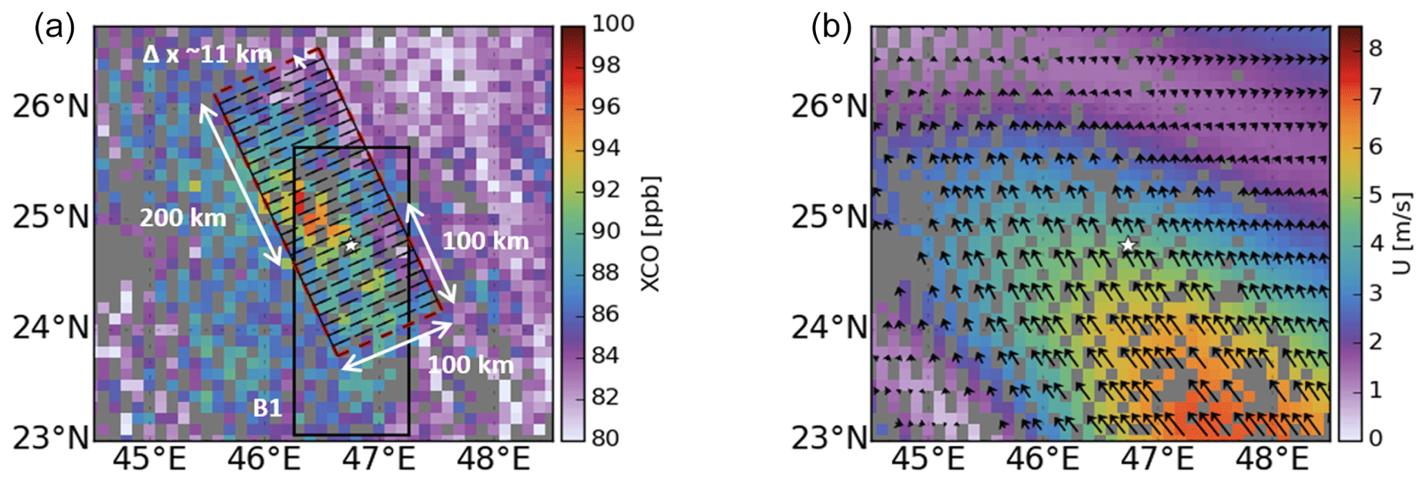
Figure 1TROPOMI-derived XCO (a) and average wind speed and wind direction from the surface to the top of the boundary layer (b) derived from the CAMS global reanalysis eac4 data at the TROPOMI overpass time over Riyadh for 4 August 2018. The white star represents the center of Riyadh. The black box (B1), with a dimension of 300×100 km2, is rotated in the average wind direction at a 50 km radius from the center of Riyadh at the TROPOMI overpass time, resulting in the red box. For the calculation of cross-directional averaged NO2 and CO, the red box is divided into 29 smaller cells with the width (Δx) ∼ 11 km. For this, TROPOMI-derived XCO is gridded at .
The components of NOx (NO and NO2) have short lifetimes during daytime because of the photo-stationary equilibrium exchanging NO and NO2 into each other. For this reason, we estimate the lifetime of their sum (NOx), which is determined largely by the reaction with OH. In earlier work with satellite NO2 data, the Jet Propulsion Laboratory (JPL) high-pressure limit was used as the rate constant to represent the first order loss of NO2 (Beirle et al., 2011; Lama et al., 2020; Lorente et al., 2019). However, we found this approximation to be too crude and therefore apply the full IUPAC-recommended pressure-dependent formula for the second order rate constant. Supplement Fig. S4 shows the difference between the three rate constants, i.e., JPL high-pressure limit, JPL second order and IUPAC second order, confirming the importance of accounting for the pressure dependence.
WRF output for the third domain is interpolated spatially and temporally to the footprints of TROPOMI. The interpolated WRF NOx tracers are converted to NO2 using the conversion factor derived from the CAMS reanalysis, accounting for its spatial and temporal variation (for the names and functions of tracers, see Table 1). The averaging kernel available for each TROPOMI CO and NO2 observation is applied to the WRF output after interpolation to the vertical layers of the TROPOMI retrieval. To compare WRF output to TROPOMI, WRF-derived XNO2(XNO2 WRF) is calculated by combining the NO2 tracer that accounts for the OH effect (XNO2 (emis,OH)) and the CAMS NO2 background (XNO2 Bg) (see Figs. S5 and S6). Similarly, the CO emission tracer (XCOemis) is added to the CAMS CO background (XCOBg) to calculate WRF-simulated XCO (XCOWRF) (see Figs. S7 and S8).
2.5 ratio calculation using box rotation
The variation of the ratio in the downwind city plume is calculated as a function of distance x from the city center in a downwind direction. We select days with an average wind speed (U) in the range of 3.0 m s−1 (Beirle et al., 2011) .5 m s−1 (Valin et al., 2013) within a 50 km radius from the center of Riyadh (24.63∘ N, 46.71∘ E). The horizontal distribution of EDGAR emissions over Riyadh is used within this 50 km radius (Fig. S9). A total of 95 d in summer and 70 d in winter meet the wind speed criteria over Riyadh for the ratio calculation. The boundary layer average wind speed and direction are calculated using the CAMS global reanalysis eac4 (retrieved at https://ads.atmosphere.copernicus.eu/cdsapp#!/dataset/cams-global-reanalysis-eac4?tab=_form, last access: 1 August 2020) at a spatial and 3 h temporal resolution. For this, the CAMS wind vector is spatially and temporally interpolated to the central coordinate of TROPOMI pixels.
To compute the ratio as function of the downwind distance x, TROPOMI and WRF data have been re-gridded at . A box (B1) is selected with a width of 100 km, from 100 km in upwind to 200 km in downwind direction of the city center (see Fig. 1a). The dimension of the box is motivated by multiple TROPOMI overpasses over Riyadh, showing NO2 and CO enhancements advected downwind over a ∼ 200 km distance without other large sources of NO2 and CO within a 100 km radius of the city center (see Fig. 1a). Figure 1b shows the boundary layer averaged wind speed and wind direction over Riyadh, indicating flow towards the northeast on 4 August 2018. The box is rotated for every TROPOMI overpass, depending upon the daily average wind direction within a 50 km radius from the center of Riyadh, as shown in Figs. 1a and S10. The rotated box B1 is divided into N rectangular boxes, orthogonal to the wind direction with length (Δx) ∼ 11 km (see Figs. 1 and S10). The XNO2 and XCO grid cells that fall within the N rectangular boxes are selected to derive zonally averaged XNO2 and XCO for summer and winter.
Unlike the enhancements over the city, ΔXNO2 and ΔXCO become smaller than retrieval uncertainties at large distance from the city, where the ratio ΔXNOXCO becomes ill defined. Therefore, we decided to use the ratio of mean XNO2 and XCO instead of enhancements over the background. To analyze the influence of atmospheric transport and the OH sink on the WRF-derived ratio, two different ratios are derived: (1) , named “ratiowithout OH”, and (2) , named “ratiowith OH” (see Table 1). The CAMS background accounts for the balance between regional source and sink in CTMs, so it is excluded to analyze the influence of atmospheric transport on the ratio. For the comparison between TROPOMI and WRF, the CAMS backgrounds are included in “WRF ratio” () (see Table 1). The comparison of WRF ratio to TROPOMI ratio and the contribution of its components are presented in Sect. 3.2.
2.6 OH estimation: satellite data only
In the EMG method, following Beirle et al. (2011), 2D NO2 column density maps are assigned to eight equal wind sectors, spanning 360∘ for summer and winter; 1D column densities per wind sector are computed by averaging in a cross-wind direction. This way, average NO2 column density functions of the downwind distance to the city center have been constructed for summer and winter (see Fig. S11). Using the EMG method, as in Beirle et al. (2011), the e-folding distance (x0) and NO2 emissions have been estimated. The NO2 lifetime is derived by dividing x0 by the average wind speed (5.46 and 5.24 m s−1 for winter and summer, respectively) and is provided in Table 2. The OH concentration is derived from the inferred NO2 lifetime using the IUPAC second order rate constant (for details, see Text S2 and S3 in the Supplement). Rate constants at the time of TROPOMI overpasses are obtained from WRF by averaging the IUPAC second order rate constant from the surface to the top of the planetary boundary layer (PBL). The PBL height at the time TROPOMI overpass has been taken from WRF. EMG-derived NO2 emissions are also converted to NOx emissions using the CAMS-derived conversion factor. Summer- and winter-averaged CAMS-derived conversion factors for the box of 300 km × 100 km are 1.28 and 1.31, respectively.
2.7 OH estimation: WRF optimization
To jointly estimate the NOx and CO emissions as well as the OH concentration from the TROPOMI data, a least-squares optimization method is used. This method fits the model to the data by minimizing a cost function (J) (see Text S4 for details). The reaction of NO2 with OH introduces a non-linearity in the OH optimization. To account for this non-linearity, we linearize the problem around the a priori starting point using the small perturbations (10 %) Δbackground, Δemission and ΔOH. The non-linear model is fitted to the observations by optimizing scaling factors fBg, femis, fOH to the perturbation functions Δbackground, Δemission and ΔOH, respectively. This process is repeated iteratively, updating the linearization point and re-computing the perturbation functions. The scaling factors femis, foh and fbg represent the modification of the prior in percentage change.
We estimate OH by optimizing WRF with TROPOMI in two ways: (1) optimizing the simulated ratio using TROPOMI-derived ratios, named as “ratio optimization”, and (2) optimizing NO2 and CO separately using TROPOMI-derived XCO and XNO2, named as “component-wise optimization”. First, the ratio optimization is described, followed by the component-wise optimization. Optimized ratios are derived as follows:
Here, FTROPOMI is the TROPOMI-derived ratio, F is the WRF ratio, is the change in F due to an increase in the NO2 emission by 5 % and a decrease in the CO emission by 5 % ( 10 %), is the change in F due to an increase in OH by 10 %, and is the change in F due to an increase in the XNO2 background by 5 % and a decrease in the CO background by 5 %. XNO2 (emis, OH) is the contribution of city NOx emissions to XNO2, accounting for the OH sink. XNO2 Bg is the NO2 background. XCOemis is the contribution of the EDGAR city CO emissions to XCO, and XCOBg is the CO background derived from CAMS. XNO2 WRF and XCOWRF are the WRF-derived XNO2 and XCO, respectively. is the contribution of city NOx emissions to XNO2 after increasing CAMS OH by 10 %. The scaling factors femis, fOH and fBg obtained from the ratio optimization have been divided by 10 because and are defined as the change in F due to modification of emission, OH and background by 10 %.
Although the ratio optimization is sensitive to the emission ratio and the OH sink of NO2, it is not sensitive to the absolute emissions of CO and NO2. Therefore, we performed component-wise optimizations for XCO and XNO2 to optimize absolute emissions. We also compare the OH factor obtained from the ratio optimization and component-wise optimization to test the robustness of the method. The optimized XNO2 is derived using Eq. (12). XCO is optimized using the same equation but without considering the OH sink (see Appendix B).
Here, XNO2 TROPOMI is the TROPOMI-derived XNO2, XNO2 WRF is the WRF XNO2. ΔXNO2 emis is the change in XNO2 due to an increase in emissions by 10 %, ΔXNO2 OH is the change in XNO2 due to an increase in CAMS OH by 10 %, and ΔXNO2 Bg is a change in the background XNO2 by 10 %. The scaling factors femis, fOH and fBg are divided by a factor 10 because ΔXNO2 emis, ΔXNO2 OH and ΔXNO2 Bg are defined as 10 % changes in NOx emission, OH and background level.

Figure 2Comparison between XNO2 (a, c) and XCO (b, d) from TROPOMI and WRF over Riyadh, averaged over June to October 2018. Panels (a) and (b) show TROPOMI data, and panels (c) and (d) show the corresponding co-located WRF results. XNO2 WRF is derived by adding XNO2(emis, OH) and XNO2 Bg. XCOWRF is derived by adding XCOemis and XCOBg. The white star represents the center of the city. TROPOMI and WRF results are gridded at .
3.1 XNO2 and XCO over Riyadh
In this subsection, we compare WRF-derived XCOWRF and XNO2 WRF with TROPOMI for summer (see Fig. 2) and winter (see Fig. S12) over Riyadh. TROPOMI and WRF-derived XCO and XNO2 are averaged from June to October 2018 for summer and November 2018 to March 2019 for winter in a domain of 500×500 km2 centered around Riyadh. The comparison for summer in Fig. 2 shows TROPOMI NO2 after replacing the TM5-based tropospheric AMF with WRF profiles, as described in Visser et al. (2019). The enhancement of XNO2 and XCO over Riyadh due to urban emissions is clearly separated from the background for TROPOMI and WRF, showing that the city of Riyadh is well suited to investigating the use of the ratio to quantify OH in urban plumes. Due to the longer lifetime of CO, the TROPOMI-observed XCO plume extends further in the southeast direction compared to XNO2. Figure 2 shows that our WRF simulations are able to reproduce the TROPOMI-retrieved XNO2 (r2=0.96) and XCO (r2=0.78) plumes, confirming that WRF-derived is suitable for the optimization of CTM-derived OH concentrations using TROPOMI data. XNO2 WRF is higher by 25 % compared to TROPOMI in the city center. In the background, XCOWRF shows a similar spatial distribution as TROPOMI XCO, but the values are higher by 5 % to 10 % (see Fig. 2). Close to the city center, XCOWRF is ∼ 5.7 % higher than TROPOMI XCO. In EDGAR 2011, emission sources are located in the center of Riyadh (see Fig. S9). However, as noted by Beirle et al. (2019), they extend to a larger part of the city in reality. This difference in spatial distribution leads to higher XNO2WRF and XCOWRF close to the center of Riyadh compared to TROPOMI.
In winter, the wind direction is predominantly from the southeasterly sector in WRF and TROPOMI (see Fig. S12). The spatial distribution of XCOWRF (r2=0.73) and XNO2 WRF (r2=0.88) matches quite well with TROPOMI. Therefore, the difference between summer and winter should offer the opportunity to quantify the seasonality in emissions and OH concentrations over Riyadh. In winter, XCOWRF is ∼ 5 % to 10 % higher than TROPOMI, while XNO2WRF is higher by 40 % to 50 %. The difference could either point to uncertainties in the emission ratio, uncertainties in the NO2 lifetime or inaccuracies in the background. By quantifying OH, we can evaluate these explanations (see Sect. 3.3). XNO2 WRF is higher by 20 % in winter than in summer. Contrarily, TROPOMI NO2 is lower by ∼ 30 % in winter (Fig. S12) compared to summer (Fig. 2). Again, to disentangle the role of changing sources and sinks, we need an independent estimate of OH.
3.2 The ratio and OH
Before comparing TROPOMI- and WRF-derived ratios, we first analyze the influence of atmospheric transport and the OH sink on the WRF-derived ratio. To do this, three ratios are used: (1) ratiowithout OH, (2) ratiowith OH, and (3) WRF ratio (see Table 1). As seen in Figs. 3, S13 and S14, WRF is able to reproduce the TROPOMI-observed downwind evolution of XNO2 and XCO in summer and winter. The peak of the XNO2 and XCO plumes is shifted away from the city center due to the balance between the accumulation of urban emissions in the atmospheric column and atmospheric transport (Lorente et al., 2019).
As expected, ratiowithout OH shows an approximately straight line when the background is removed because transport influences NO2 and CO in the same way and therefore cancels out in the ratio (see Fig. 3b). The ratiowith OH however, shows an approximately Gaussian relation with distance due to the influence of the sink on NO2. This comparison demonstrates the sensitivity of the relation between the ratio and downwind distance to the NO2 lifetime, which we want to exploit to quantify OH. When including the background, the shapes of the functions in Fig. 3c change (not shown) because the relative weights of the background and city contributions to the ratio vary with distance from the city center. In summer, the WRF ratio is higher by ∼ 15 % close to the center-of-city TROPOMI due to the overestimation of XNO2 WRF in WRF (see Fig. 3d). However, in the downwind plume, at a distance of 100 km, WRF ratio is higher by 20 % to 50 % compared to TROPOMI.
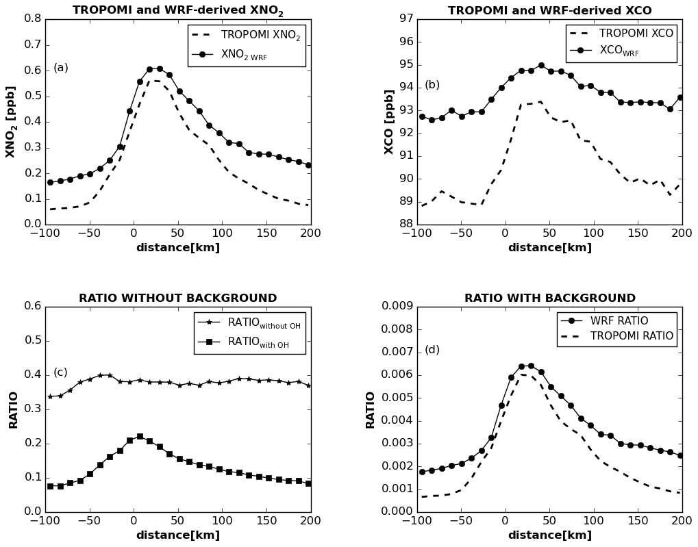
Figure 3Comparison of WRF and TROPOMI averaged across the wind for each small box (a) XNO2, (b) XCO, (c) WRF ratio () without CAMS background and (d) WRF ratio (), with background and TROPOMI as a function of distance to the center of Riyadh for summer (June to October 2018).
In winter, ratiowithout OH and ratiowith OH show relations with downwind distance that are similar to summer, confirming that an OH sink leads to a Gaussian structure of the ratio (see Fig. S14). The winter WRF ratio is 40 % to 60 % higher than TROPOMI due to the overestimation of XNO2 by 40 % to 50 %. The WRF ratio close to the center of the city is also 20 % higher in winter than in summer due to higher winter XNO2 WRF (see Figs. S12 and S15). In contrast, TROPOMI shows a higher ratio in summer compared to winter (see Fig. S15). These differences between TROPOMI- and WRF-derived ratios offer an opportunity to address uncertainties in CTM-computed urban OH and emission inventories, which will be explored next.
3.3 WRF optimization using synthetic data
To translate the discrepancies between TROPOMI- and WRF-derived ratios of Sect. 3.2 into implied differences in emissions, OH and background, the least-squares optimization method has been used as described in Sect. 2.7. Before optimizing WRF using TROPOMI, pseudo-data experiments in WRF have been carried out to test if the optimization method is capable of recovering true emissions and OH levels. To this end, changes in OH concentrations, emissions and background by known scaling factors have been applied to the WRF prior simulation to create a synthetic dataset. This process is repeated multiple times to create thousands of synthetic datasets. Subsequently, the scaling factors are obtained in the inversion procedure. These tests reveal that the estimation errors for femis, fOH and fBg are less than 2.5 % (see Fig. S16). This confirms that the least-squares optimization method works, with two iterations leading to a sufficient accuracy, and can be used to estimate emissions and OH from TROPOMI data. Using TROPOMI data, estimation errors for femis, fOH and fBg are expected to be higher due to atmospheric transport errors, simplified chemistry, and XCO and XNO2 retrieval uncertainties. These errors did not play a role in the pseudo-data experiments, in which perfect transport and sampling were assumed.
To obtain a more realistic estimate of the uncertainty in least-squares-optimized OH, TROPOMI data have been replaced by NO2, CO and the ratio derived from WRF-Chem using the Carbon Bond Mechanism Z (CBM-Z) gas-phase chemical mechanism (Zaveri and Peters, 1999). EDGAR-based VOCs, NOx and CO emissions have been used in combination with boundary conditions for NO, NO2, CO and ozone (O3) from CAMS to run WRF-Chem for 17 August and 18 November 2018, representing a summer and winter day, respectively. For 17 August 2018, the ratio and XNO2 optimization increase the CAMS-based prior OH of 1.19×10⁷ molec. cm−3 by 15.7 % and 13.4 %, respectively (see Fig. S17). In the fully coupled online chemistry with WRF simulation, the boundary layer averaged OH for the box of 300 km × 100 km amounts to 1.33×10⁷ molec. cm−3, which is < 5 % lower than the optimized OH value that is derived using our method. The optimized NOx and CO emissions differ by < 11 % from the emission input used in the full-chemistry-version WRF. In winter, the optimization increases CAMS-based OH of 1.03×10⁷ molec. cm−3 by 19.4 %. The OH derived from WRF with full online chemistry is 1.07×10⁷ molec. cm−3 and lower by 15.2 % than the optimized OH value. The component-wise optimization increases the EDGAR NOx and CO emissions by 23.1 % and 10.5 %, respectively (see Fig. S18). Overall, the uncertainty in optimized NOx, CO emission and OH derived from this test is < 11 % in summer and 10 % to 23 % in winter. Since the lifetime of NOx is determined by other reactions in addition to the oxidation to HNO3 considered in our method, it is expected to overestimate the real OH value. The test using WRF full chemistry confirms that this is indeed the case. The uncertainties for OH, NOx emission and CO emission are in good agreement with the CLASS computations explained in detail in Text S6.
3.4 WRF optimization using seasonally averaged TROPOMI data
The results for summer are summarized in Fig. 4, showing the optimized fit to the TROPOMI data as well as the corresponding scaling factors femis, fOH and fBg that are estimated. The optimized emission, OH and Bg obtained from the second iteration are divided by the prior to derive the femis, fOH and fBg (see Text S5 for details). The convergence of the iterative procedure is shown in Figs. S19 and S20. The estimated uncertainties for the scaling factors femis, fOH and fBg are derived by summing the contribution of wind speed, length and width of the box, NO2 bias, CO bias, and the different pathways of NOx loss in quadrature (see Text S6, Tables S1 and S2). For summer and winter, the uncertainties of the optimized OH concentrations are < 17 % and < 29 %, respectively. For NOx and CO emissions, the uncertainty is < 29 % in summer and winter. Figure 4a shows WRF ratios for summer in comparison to TROPOMI, before and after optimizing the OH concentration. The optimized WRF ratios fit the TROPOMI ratios well, with X2=0.1 (for the derivation of X2, see Text S7). The prior and optimized emission ratios, OH concentrations and background ratios obtained from component and ratio optimizations for summer and winter are provided in Table S4. According to the ratio optimization, the emission ratio and CAMS OH are underestimated by 155 ± 26 % and 32 ± 5.3 %, respectively (see Table S4). The optimized CAMS background ratio is lower by 70 ± 6.5 % compared to prior. It should be realized here that the ratio optimization does not estimate the absolute emission of NO2 and CO, only their ratio.

Figure 4Comparison between TROPOMI and WRF, before and after optimization for summer (averaged over June to October 2018) (a) ratio, (b) XNO2 and (c) XCO in comparison to TROPOMI; fOH, femis and fBg are optimized scaling factors obtained iteratively for OH, emissions and background by the least-squares optimization method; femis, fOH and fBg are derived by accounting the total change in emission, OH and background using the corresponding scaling factors obtained from the first and second iterative steps. The unit of the scaling factor is in percent (%).
To derive the absolute emission, we performed component-wise optimizations of WRF-derived XCOWRF and XNO2 WRF. Optimized XCOWRF and XNO2 WRF fit well to the TROPOMI data (see Fig. 4b and c). In the XNO2 optimization, the EDGAR NOx emission is increased by 42.1 ± 8.4 %, and the CAMs background is reduced by 75.9 ± 10.0 %. CAMS OH is increased by 28.3 ± 3.9 %, which is close to the results obtained from the ratio optimization (see Table S4). In the XCO optimization, EDGAR CO emissions are roughly doubled, and the background is reduced by 4.5 ± 0.7 % compared to CAMS (see Table S4).
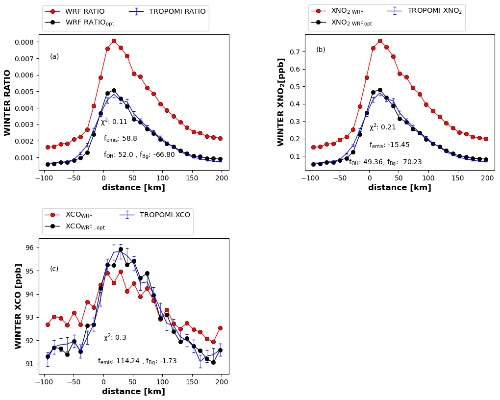
The summer optimized emission ratio derived from the component-wise optimization is 0.55 ± 0.09. The optimized emission ratio from ratio optimization is larger by factor 3.6 compared to component-wise optimization (see Table S4). The difference between two estimates can be explained by different constraints on the solution in the two methods. In particular, the ratio inversion allows emission adjustment in a fixed relation between NO2 and CO emissions, whereas the component-wise has the full flexibility to adjust CO and NO2 emissions. The ratio over a city is the sum of the contributions of the background and the city emissions. The relative weight of the two is determined by the absolute background levels and absolute emissions of CO and NO2. Therefore, the emission ratio estimated by ratio optimization is sensitive to the XNO2 Bg. However, the difference between the two estimates is larger than expected but does not affect the OH estimation. Lama et al. (2020) inferred an emission ratio over Riyadh of 0.47 ± 0.1 for 2018 from TROPOMI, favoring the Monitoring Atmospheric Chemistry and Climate and CityZen (MACCity) emission ratio over that of EDGAR. The optimized emission ratio obtained from component-wise optimization is consistent with Lama et al. (2020) and with MACCity summer emissions. This shows that, for the accurate estimation of the emission and emission ratio, the component-wise optimization method is preferable.
Figure 5 presents optimization results for winter, where optimized WRF is in similar good agreement with TROPOMI as for summer, with X2=0.11. For winter, the ratio optimization increases the emission ratio by 58.8±33 % and OH by 52.0 ± 14 %. The ratio and component-wise optimizations again show similar OH adjustments, demonstrating the robustness of our method. The background ratio is reduced by 66.8 ± 11 %. The XNO2 optimization reduces the EDGAR NOx emission by 15.45 ± 4.1 % and the CAMS background by 70.2 ± 6.1 %. For XCO, the WRF XCOBg is reduced by 1.74 ± 0.1 % in combination with a doubling of the EDGAR CO emission. The optimized emission ratio () derived from component-wise optimization is 0.36, which is 4 times lower than the optimized emission ratio obtained from ratio optimization (see Table S4).
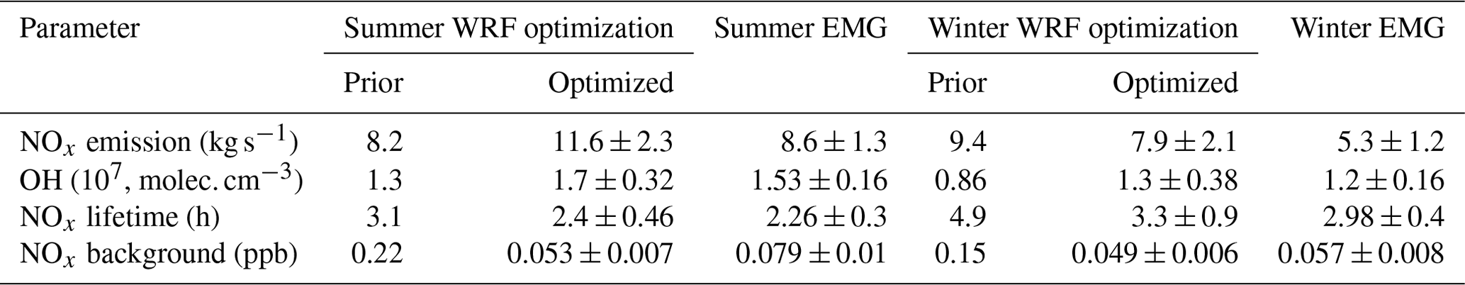
Table 2Overview of WRF-optimized OH and NOx emissions for Riyadh and comparison to the EMG method. The estimated uncertainty for EMG- and WRF-derived NOx emissions and OH concentrations is the sum of the contribution of wind speed, length and width of the box, NO2 bias correction, CO bias, and the different pathways of NOx loss provided in Tables S1, S2 and S3.
3.5 WRF optimization using a single TROPOMI overpass
To demonstrate the application of our WRF optimization method to a single TROPOMI overpass, results are presented in this subsection for 18 August 2018. This date was selected for clear-sky conditions, with most of the TROPOMI NO2 and CO pixels passing the data quality filter. During this day, the urban plume was transported in a southwestern direction over Riyadh. The spatial distribution of XNO2 WRF (r2=0.76) and XCOWRF (r2=0.65) matches quite well with TROPOMI (see Fig. S21). The optimized ratio, XNO2 and XCO for a single day fit well with TROPOMI (X2=0.1, 0.3 and 0.7), comparable to the summer-averaged plumes, indicating that the optimization method can be applied to a single TROPOMI overpass. The ratio optimization increases the emission ratio and CAMS OH by 111 ± 18.4 % and 37.9 ± 6.2 %, respectively, whereas the background is reduced by 51.5 ± 5.2 % (see Fig. S22a). The XNO2 optimization increases the EDGAR NOx emission by 25.5 ± 5.1 % and CAMS OH by 32.3 ± 4.4 %, whereas the NOx background is reduced by 54.4 ± 7.0 % (see Fig. S22b). The CO optimization doubles the EDGAR CO emission and reduces the background by 6.1 ± 0.97 % (see Fig. S20c). The optimized NOx and CO emissions for 18 August are 8.9 ± 1.7 and 18.9 ± 4.0 kg s−1, respectively, and differ by < 25 % from the summer optimized emission (see Tables 2 and S5). The optimized OH derived from a single TROPOMI overpass is 1.73×10⁷ ± 0.3 molec. cm−3 and differs by < 5 % from the summer-averaged OH, i.e., 1.7×10⁷ ± 0.3 molec. cm−3, confirming that the method yields realistic results for a single overpass.
3.6 WRF optimization vs. the EMG method
To investigate the consistency between our method and the EMG method, the derived NOx lifetimes, emissions and OH concentrations using both methods are listed in Table 2 for winter and summer. Our optimization and the EMG method agree well on the seasonal change in NOx emission and OH concentration. Both methods result in higher NOx emissions and shorter lifetimes in summer and lower NOx emissions and longer lifetimes in winter. Riyadh has dry and warm summer days, and the increase in power consumption due to the use of air conditioning contributes to the higher emissions in summer than in winter (Lange et al., 2022). During the summer, EMG and the WRF optimization method both increase the NOx emission and OH concentration compared with the prior. The sizes of the NOx emission and OH concentration increase, obtained using the WRF optimization method, which is higher than the EMG method by 10 % to 29 %. However, the differences between the EMG method and the component optimization method are smaller compared to the uncertainties of the emission and OH concentration derived for the optimization method. For winter, the difference between the EMG and WRF-optimized results are smaller than the difference between the EMG results and the prior. The NOx emission after optimization differs from the EMG method by 33 %. Optimized OH concentration and NOx lifetime differ by < 10 % compared to the EMG method. In general, the difference between the EMG and optimization results is within the uncertainty range of 20 % to 30 %, confirming their consistency and strengthening the confidence in the estimates that are obtained from TROPOMI data. In contrast to the EMG method, the optimization method can be used for a single TROPOMI overpass (see Sect. 3.5) and does not require yearly averaged NO2 data, allowing analysis of day-by-day OH, NOx and CO emissions (see Sect. 3.3). Segregation and averaging of NO2 urban plumes by wind sector is not required in the optimization method. The effect of transport cancels out in taking the ratio, and loss of NO2 is mostly governed by OH during the midday. In this study, NOx emission and OH concentration are estimated iteratively, whereas the EMG method arrives at the solution in a single step. However, since our optimization method requires a WRF model simulation, it is computationally more expensive. Uncertainties in transport may create mismatches with the satellite observations, leading to errors in the optimized fit. This influences the quality of derived emission estimates (Dekker et al., 2017). Therefore, finding a simplified approach using satellite data to derive the emission ratio and to estimate OH concentration in urban plumes will be our focus in the future. In the future, the accuracy of our method can be further improved by accounting for other NOx removal pathways.
3.7 WRF optimized emissions and emission trends
It should be realized that the a priori EDGAR emissions and TROPOMI optimized estimates represent different years (2012 and 2018, respectively). To check whether the emission differences that are found may be explained by trends in emissions, we compare EDGARv5.0 2012 NOx and CO emissions with 2018, accounting for seasonal and diurnal emission variations using temporal emission factors from van der Gon et al. (2011). EDGAR 2018 NOx and CO emissions are derived by linear extrapolation using emissions from 2000 to 2015 (see Fig. S23). For summer, midday NOx emissions, the EDGAR emissions increased by 16.7 % from 2012 to 2018, which is lower than our optimization results. For winter, midday NOx emissions increased in EDGAR by 15.2 % from 2012 to 2018, whereas the WRF optimization yielded reductions of 15.6 %. In EDGAR, summer and winter CO emissions increased from 2012 to 2018 by 38.5 %. However, the WRF optimization suggests that the EDGAR CO emissions for summer and winter need to be doubled (see Table S5). Borsdorff et al. (2018b) mentioned that EDGAR CO emissions have to be increased significantly to match with TROPOMI CO observations over middle eastern cities such as Tehran, Yerevan, Tabriz and Urmia. Overall, this points to a significant uncertainty in the EDGAR emission inventory at the city scale.
To test the accuracy of the linear extrapolation of EDGAR data, we compare the relative change in NOx and CO emissions in 2012 to 2018 using CAMS Global (CAMS-GLOB) anthropogenic v4.2 emission datasets (https://ads.atmosphere.copernicus.eu/cdsapp#!/dataset/cams-global-emission-inventories?tab=overview, last access: 15 June 2021). CAMS-GLOB shows that, for summer and winter, NOx emissions increased by 26 % from 2012 to 2018, which is higher than EDGAR by a factor of 1.7. CAMS-GLOB-based summer and winter CO emissions increase by 20 % from 2012 to 2018, which differs by ∼ 40 % compared to EDGAR. In general, the relative increase in CO and NOx emissions from EDGAR and CAMS-GLOB is much smaller compared to the difference with our optimization method.
The TROPOMI-retrieved ratio is useful for estimating midday OH over isolated localized sources, such as the city of Riyadh, showing a clear contrast between the urban plume and the background. Such TROPOMI-derived OH estimates offer a new opportunity to evaluate urban photochemistry in chemistry transport models. OH depends non-linearly on NOx and VOC emissions, meteorological conditions, etc. (Sillman et al., 1990), which vary substantially between cities that are monitored by TROPOMI. Therefore, the application of our method to the global and multi-year dataset that is available could contribute substantially to the understanding of urban photochemistry and the development of effective pollution mitigation strategies. In addition, the method requires local sources with NO2 and CO emissions that are large enough to be detected by TROPOMI. Especially in European cities with lower CO emission, where TROPOMI cannot detect the CO enhancement along with NO2, this method cannot be applied.
We realize that our method only considers the first order loss of NO2 by OH-forming HNO3. In reality, the NO2 lifetime is influenced by more spatially and temporally varying factors such as temperature, ozone and radiation (Lang et al., 2015; Romer et al., 2018). In cities, the loss of NO2 via the formation of alkyl and multifunctional nitrates (RONO2) is also an important reaction influencing the lifetime of NO2 (Browne et al., 2013; Sobanski et al., 2017). For CO, secondary production from short-lived volatile organic compounds can also play an important role in urban pollution plumes. The application of full chemistry that includes all the sources and losses of NO2 and CO could therefore further improve the accuracy of OH estimates.
For cities at higher latitudes, especially in winter, it becomes more critical to account for the contribution of other pathways of NOx loss than OH oxidation. Isolated tropical and subtropical cities are therefore best suited for application of our current method.
A sensitivity test has been performed in which XNOx, Bg is lost by OH. In this case, the optimized NOx emission and OH for summer and winter differ by < 7 % from the default method, where the background is treated as an inert tracer (see Table S6). Furthermore, a sensitivity test has been performed in which the prior emission has been changed. The optimized emission varied by < 5 %, demonstrating robustness of the method to the choice of prior (see Fig. S24). This also indicates that the optimization method can be used to study emission changes. Figure S25 shows that road transport, power plants and manufacturing industries are the largest pollutant emitter over Riyadh (Beirle et al., 2019). In this study, NOx and CO anthropogenic emissions are introduced at the surface, whereas the emission height of different sources is expected to vary in reality. The different emission heights for NOx and CO emission sources can also influence the result. In the future, realistic emission heights should also be incorporated in WRF for accurate estimation of OH. Moreover, the temporal emission factors that have been used by van der Gon et al. (2011) are based on European countries. The comparison of van der Gon et al. (2011) with the Copernicus Atmosphere Monitoring Service TEMPOral profiles (CAMS-TEMPO) (Guevara et al., 2021) suggests that temporal emission factors for weekend road transport and monthly residential combustion are different in Riyadh compared to European countries. CAMS-TEMPO is expected to provide a more accurate representation of emission variation due to the information on temporal and spatial variations that is included. Road transport CO emissions are the largest contributor by ∼ 75 % to the total emissions over Riyadh, whereas NOx emissions from the road contribute by 24 % to the total NOx emission. Residential combustion has the smallest contribution of ∼ 0.3 % to 0.4 % to total NOx and CO emissions (see Fig. S25). In the future, the application of accurate diurnal emission factors for road transport (see Fig. S26) can further improve the accuracy of urban OH concentrations estimated using TROPOMI-derived ratios. In addition, the seasonality for NOx and CO emissions is different in Riyadh than in Europe, which should also be accounted for in future studies.
In this study, a new method is presented for estimating OH concentrations in urban plumes using TROPOMI-observed ratios in combination with WRF simulations of the downwind pollution plume of large cities. Our new method has been tested for the city of Riyadh using synthetic as well as real TROPOMI data. Seasonal emissions and OH concentrations have been estimated for summer (June to October 2018) and winter (November 2018 to March 2019). WRF is well able to reproduce the spatial distribution of TROPOMI-retrieved XNO2 and XCO plumes over Riyadh during the summer and winter seasons. However, before the optimization, WRF overestimates XNO2 by 15 % to 30 % in summer and 40 % to 50 % in winter compared to TROPOMI. In both seasons, TROPOMI XCO agrees within 10 % with WRF. The WRF-derived ratio is higher by 15 % to 30 % in summer and 40 % to 60 % in winter compared to TROPOMI, explained mostly by differences in XNO2.
The differences between WRF and TROPOMI observations have been used to optimize emissions and the NO2 lifetime. To this end, scaling factors for the city emissions, OH and the background level have been optimized iteratively using a least-squares method. Ratio and component-wise optimizations have been compared to test the overall consistency of the method. In summer, the ratio and XNO2 optimization for XNO2 suggest that the OH prior from CAMS is underestimated by 32 ± 5.3 % and 28.3 ± 3.9 %, respectively . The OH estimates obtained from the ratio and NO2-only optimization differ by < 10 %, demonstrating the robustness of the method. Summertime emissions of NOx and CO from EDGAR are increased by 42.1 ± 8.4 % and 101 ± 21 %. For winter, the ratio and component-wise optimizations increase OH by ∼ 52 ± 14 % to fit TROPOMI-inferred ratios. In the optimization of winter data, NOx emissions are reduced by 15.5 ± 4.1 %, and CO emissions are doubled. In the future, the remaining differences between TROPOMI observations and WRF simulations could be reduced further by the use of precise temporal and monthly emission factors, emission heights and full chemistry to account for secondary sources and sinks of CO and NO2.
TROPOMI-inferred OH concentrations obtained from the least-squares optimization method have been compared to the EMG method. For the summer and winter, the optimized OH concentrations differ by 10 % between the two methods. These results confirm that urban emissions and OH concentrations can be estimated robustly from TROPOMI data. With our method, single TROPOMI overpasses can be used to estimate OH, whereas the EMG method requires averaging of urban NO2 plumes by wind sector. The iterative approach allows one to test the factors, i.e., femis, foh and fbg, obtained from the optimization method, whereas the EMG method does not allow such flexibility.
An important remaining uncertainty is the bias correction of the TROPOMI XNO2 retrieval. Following the recommended procedure, the air mass factor AMF is recalculated by replacing the tropospheric AMF based on TM5, which is provided with the data, with WRF-Chem. The TROPOMI XNO2 bias correction increases the mixing ratio in the urban plume of Riyadh by 5 % to 10 % in summer and 25 % to 30 % in winter. The background is less affected by the bias correction. Without TROPOMI XNO2 bias correction, the uncertainty in the scaling factor for OH can vary up to 20 % and up to 60 % for NOx emissions over Riyadh.
The air mass factor (AMF) used in the retrieval of TROPOMI XNO2 has been re-calculated by replacing the tropospheric AMF, calculated from the NO2 column simulated by TM5, with its WRF-Chem equivalent, as described by Lamsal et al. (2010) and Boersma et al. (2016), using the following Eq. (A1):
where Mtrop,WRF and Mtrop,TM5 are the tropospheric air mass factors derived from WRF and TM5, respectively. Atrop,l is the tropospheric averaging kernel, ranging from the surface to the uppermost layer of the troposphere in the TM5 model (l). xl,WRF is the equivalent NO2 column density in model layer l, based on WRF. Atrop in Eq. (A1) is derived using , where M and Mtrop are the total and tropospheric AMFs, respectively. Finally, the bias-corrected NO2 vertical column density is computed using
where NO2 is the TROPOMI tropospheric NO2 vertical column density, and NO2, bias-corrected is the bias-corrected TROPOMI tropospheric NO2 vertical column density.
The component-wise optimization of XCOWRF to estimate the emission and background of CO uses the following equations:
Here, XCOTROPOMI is TROPOMI XCO, XCOWRF is the WRF-simulated XCO accounting for emissions and background CO, XCOemis is the XCO contribution from the urban CO emission, and XCOBg is the CAMS-derived XCO background. ΔXCOemis is the change in XCO due to emission, and ΔXCOBg is the change in the XCO background level.
TROPOMI CO and NO2 data can be downloaded from https://cophub.copernicus.eu/s5pexp (ESA, 2018). EDGAR emission data are available at https://edgar.jrc.ec.europa.eu/emissions_data_and_maps (last access: 23 June 2021, Crippa et al., 2016). CAMS data can be downloaded from https://ads.atmosphere.copernicus.eu/cdsapp#!/dataset/cams-global-reanalysis-eac4?tab=_form (last access: 1 November 2020, Inness et al., 2019).
WRF simulations outputs are available at https://doi.org/10.5281/zenodo.5752219 (Lama et al., 2021).
The supplement related to this article is available online at: https://doi.org/10.5194/acp-22-16053-2022-supplement.
SL performed the data analysis and data interpretation and wrote the paper. SH supervised the study. SH, FKB, IA, MK and HACDG discussed the results. All co-authors commented on the paper and improved it.
At least one of the (co-)authors is a member of the editorial board of Atmospheric Chemistry and Physics. The peer-review process was guided by an independent editor, and the authors also have no other competing interests to declare.
Publisher's note: Copernicus Publications remains neutral with regard to jurisdictional claims in published maps and institutional affiliations.
We are thankful to the team that designed the TROPOMI instrument, consisting of the partnership between Airbus Defence and Space Netherlands, KNMI, SRON and TNO, commissioned by NSO and ESA. We acknowledge the free availability of the WRF-Chem model (http://www.wrf-model.org/, last access: 22 August 2019). Thanks to SURFSara for making the Cartesius HPC platform available for computations via computing grant no. 17235.
This research has been supported by the Aard- en Levenswetenschappen, Nederlandse Organisatie voor Wetenschappelijk Onderzoek (grant no. 2017.036).
This paper was edited by Bryan N. Duncan and reviewed by two anonymous referees.
Babic, L., Braak, R., Dierssen, R., Kissi-Ameyaw, J., Kleipool, J., Leloux, J., Loots, E., Ludewig, A., Rozemeijer, N., Smeets, S., and Vacanti, G.: Algorithm theoretical basis document for the TROPOMI L01b data processor Erwin Loots Quintus Kleipool, l,: S5P-KNMI-L01B-0009-SD, issue 9.0.0, https://sentinel.esa.int/documents/247904/2476257/Sentinel-5P-TROPOMI-Level-1B-ATBD, (last acess: 3 January 2020), 2019.
Beirle, S., Boersma, K. F., Platt, U., Lawrence, M. G., and Wagner, T.: Megacity emissions and lifetimes of nitrogen oxides probed from space, Science, 333, 1737–1739, https://doi.org/10.1126/science.1207824, 2011.
Beirle, S., Borger, C., Dörner, S., Li, A., Hu, Z., Liu, F., Wang, Y., and Wagner, T.: Pinpointing nitrogen oxide emissions from space, Sci. Adv., 5, 1–7, https://doi.org/10.1126/sciadv.aax9800, 2019.
Boersma, K. F., Vinken, G. C. M., and Eskes, H. J.: Representativeness errors in comparing chemistry transport and chemistry climate models with satellite UV–Vis tropospheric column retrievals, Geosci. Model Dev., 9, 875–898, https://doi.org/10.5194/gmd-9-875-2016, 2016.
Boersma, K. F., Eskes, H. J., Richter, A., De Smedt, I., Lorente, A., Beirle, S., van Geffen, J. H. G. M., Zara, M., Peters, E., Van Roozendael, M., Wagner, T., Maasakkers, J. D., van der A, R. J., Nightingale, J., De Rudder, A., Irie, H., Pinardi, G., Lambert, J.-C., and Compernolle, S. C.: Improving algorithms and uncertainty estimates for satellite NO2 retrievals: results from the quality assurance for the essential climate variables (QA4ECV) project, Atmos. Meas. Tech., 11, 6651–6678, https://doi.org/10.5194/amt-11-6651-2018, 2018.
Borsdorff, T., Hasekamp, O. P., Wassmann, A., and Landgraf, J.: Insights into Tikhonov regularization: application to trace gas column retrieval and the efficient calculation of total column averaging kernels, Atmos. Meas. Tech., 7, 523–535, https://doi.org/10.5194/amt-7-523-2014, 2014.
Borsdorff, T., Andrasec, J., aan de Brugh, J., Hu, H., Aben, I., and Landgraf, J.: Detection of carbon monoxide pollution from cities and wildfires on regional and urban scales: the benefit of CO column retrievals from SCIAMACHY 2.3 µm measurements under cloudy conditions, Atmos. Meas. Tech., 11, 2553–2565, https://doi.org/10.5194/amt-11-2553-2018, 2018a.
Borsdorff, T., aan de Brugh, J., Hu, H., Hasekamp, O., Sussmann, R., Rettinger, M., Hase, F., Gross, J., Schneider, M., Garcia, O., Stremme, W., Grutter, M., Feist, D. G., Arnold, S. G., De Mazière, M., Kumar Sha, M., Pollard, D. F., Kiel, M., Roehl, C., Wennberg, P. O., Toon, G. C., and Landgraf, J.: Mapping carbon monoxide pollution from space down to city scales with daily global coverage, Atmos. Meas. Tech., 11, 5507–5518, https://doi.org/10.5194/amt-11-5507-2018, 2018b.
Borsdorff, T., aan de Brugh, J., Pandey, S., Hasekamp, O., Aben, I., Houweling, S., and Landgraf, J.: Carbon monoxide air pollution on sub-city scales and along arterial roads detected by the Tropospheric Monitoring Instrument, Atmos. Chem. Phys., 19, 3579–3588, https://doi.org/10.5194/acp-19-3579-2019, 2019.
Browne, E. C., Min, K.-E., Wooldridge, P. J., Apel, E., Blake, D. R., Brune, W. H., Cantrell, C. A., Cubison, M. J., Diskin, G. S., Jimenez, J. L., Weinheimer, A. J., Wennberg, P. O., Wisthaler, A., and Cohen, R. C.: Observations of total RONO2 over the boreal forest: NOx sinks and HNO3 sources, Atmos. Chem. Phys., 13, 4543–4562, https://doi.org/10.5194/acp-13-4543-2013, 2013.
Burnett, R., Chen, H., Szyszkowicz, M., Fann, N., Hubbell, B., Pope, C. A., Apte, J. S., Brauer, M., Cohen, A., Weichenthal, S., Coggins, J., Di, Q., Brunekreef, B., Frostad, J., Lim, S. S., Kan, H., Walker, K. D., Thurston, G. D., Hayes, R. B., Lim, C. C., Turner, M. C., Jerrett, M., Krewski, D., Gapstur, S. M., Diver, W. R., Ostro, B., Goldberg, D., Crouse, D. L., Martin, R. V., Peters, P., Pinault, L., Tjepkema, M., Van Donkelaar, A., Villeneuve, P. J., Miller, A. B., Yin, P., Zhou, M., Wang, L., Janssen, N. A. H., Marra, M., Atkinson, R. W., Tsang, H., Thach, T. Q., Cannon, J. B., Allen, R. T., Hart, J. E., Laden, F., Cesaroni, G., Forastiere, F., Weinmayr, G., Jaensch, A., Nagel, G., Concin, H., and Spadaro, J. V.: Global estimates of mortality associated with longterm exposure to outdoor fine particulate matter, P. Natl. Acad. Sci. USA, 115, 9592–9597, https://doi.org/10.1073/pnas.1803222115, 2018.
Crippa, M., Janssens-Maenhout, G., Dentener, F., Guizzardi, D., Sindelarova, K., Muntean, M., Van Dingenen, R., and Granier, C.: Forty years of improvements in European air quality: regional policy-industry interactions with global impacts, Atmos. Chem. Phys., 16, 3825–3841, https://doi.org/10.5194/acp-16-3825-2016, 2016.
de Gouw, J. A., Parrish, D. D., Brown, S. S., Edwards, P., Gilman, J. B., Graus, M., Hanisco, T. F., Kaiser, J., Keutsch, F. N., Kim, S.-W., Lerner, B. M., Neuman, J. A., Nowak, J. B., Pollack, I. B., Roberts, J. M., Ryerson, T. B., Veres, P. R., Warneke, C., and Wolfe, G. M.: Hydrocarbon Removal in Power Plant Plumes Shows Nitrogen Oxide Dependence of Hydroxyl Radicals, Geophys. Res. Lett., 46, 7752–7760, https://doi.org/10.1029/2019GL083044, 2019.
Dekker, I. N., Houweling, S., Aben, I., Röckmann, T., Krol, M., Martínez-Alonso, S., Deeter, M. N., and Worden, H. M.: Quantification of CO emissions from the city of Madrid using MOPITT satellite retrievals and WRF simulations, Atmos. Chem. Phys., 17, 14675–14694, https://doi.org/10.5194/acp-17-14675-2017, 2017.
Delaria, E. R., Place, B. K., Liu, A. X., and Cohen, R. C.: Laboratory measurements of stomatal NO2 deposition to native California trees and the role of forests in the NOx cycle, Atmos. Chem. Phys., 20, 14023–14041, https://doi.org/10.5194/acp-20-14023-2020, 2020.
Ding, J., Miyazaki, K., van der A, R. J., Mijling, B., Kurokawa, J.-I., Cho, S., Janssens-Maenhout, G., Zhang, Q., Liu, F., and Levelt, P. F.: Intercomparison of NOx emission inventories over East Asia, Atmos. Chem. Phys., 17, 10125–10141, https://doi.org/10.5194/acp-17-10125-2017, 2017.
Ek, M. B., Mitchell, K. E., Lin, Y., Rogers, E., Grunmann, P., Koren, V., Gayno, G., and Tarpley, J. D.: Implementation of Noah land surface model advances in the National Centers for Environmental Prediction operational mesoscale Eta model, J. Geophys. Res.-Atmos., 108, 1–16, https://doi.org/10.1029/2002jd003296, 2003.
ESA: https://s5phub.copernicus.eu (last access: 21 September 2020), 2018.
Eskes, H. J., van Geffen, J., Boersma, K. F., Eichmann, K.-U, Apituley, A., Pedergnana, M., Sneep, M., Pepijn, J., and Loyola, D.: Level 2 Product User Manual Henk Eskes, S5P-KNMI-L2-0021-MA, issue 3.0.0, https://earth.esa.int/documents/247904/2474726/Sentinel-5P-Level-2-Product-User-Manual-Nitrogen-Dioxide (last access: 27 March 2019), 2018.
Flagan, R. C. and Seinfeld, J. H.: Fundamentals of Air Pollution Engineering, Prentice-Hall, Inc., Englewood CLiffs, NJ, 580 pp., ISBN 0-13-332537-7, http://resolver.caltech.edu/CaltechBOOK:1988.001 (last access: 23 January 2019), 1988.
Georgoulias, A. K., van der A, R. J., Stammes, P., Boersma, K. F., and Eskes, H. J.: Trends and trend reversal detection in 2 decades of tropospheric NO2 satellite observations, Atmos. Chem. Phys., 19, 6269–6294, https://doi.org/10.5194/acp-19-6269-2019, 2019.
Grell, G. A., Peckham, S. E., Schmitz, R., McKeen, S. A., Frost, G., Skamarock, W. C., and Eder, B.: Fully coupled “online” chemistry within the WRF model, Atmos. Environ., 39, 6957–6975, https://doi.org/10.1016/j.atmosenv.2005.04.027, 2005.
Guevara, M., Jorba, O., Tena, C., Denier van der Gon, H., Kuenen, J., Elguindi, N., Darras, S., Granier, C., and Pérez García-Pando, C.: Copernicus Atmosphere Monitoring Service TEMPOral profiles (CAMS-TEMPO): global and European emission temporal profile maps for atmospheric chemistry modelling, Earth Syst. Sci. Data, 13, 367–404, https://doi.org/10.5194/essd-13-367-2021, 2021.
Hakkarainen, J., Ialongo, I., and Tamminen, J.: Direct space-based observations of anthropogenic CO2 emission areas from OCO-2, Geophys. Res. Lett., 43, 11400–11406, https://doi.org/10.1002/2016GL070885, 2016.
Hong, S.-Y., Kim, J., Lim, J., and Dudhia, J.: The WRF single moment microphysics scheme (WSM), J. Korean Meteorol. Soc., 42, 129–151, 2006.
Hu, X. M., Klein, P. M., and Xue, M.: Evaluation of the updated YSU planetary boundary layer scheme within WRF for wind resource and air quality assessments, J. Geophys. Res.-Atmos., 118, 10490–10505, https://doi.org/10.1002/jgrd.50823, 2013.
Huijnen, V., Eskes, H. J., Poupkou, A., Elbern, H., Boersma, K. F., Foret, G., Sofiev, M., Valdebenito, A., Flemming, J., Stein, O., Gross, A., Robertson, L., D'Isidoro, M., Kioutsioukis, I., Friese, E., Amstrup, B., Bergstrom, R., Strunk, A., Vira, J., Zyryanov, D., Maurizi, A., Melas, D., Peuch, V.-H., and Zerefos, C.: Comparison of OMI NO2 tropospheric columns with an ensemble of global and European regional air quality models, Atmos. Chem. Phys., 10, 3273–3296, https://doi.org/10.5194/acp-10-3273-2010, 2010.
Huijnen, V., Pozzer, A., Arteta, J., Brasseur, G., Bouarar, I., Chabrillat, S., Christophe, Y., Doumbia, T., Flemming, J., Guth, J., Josse, B., Karydis, V. A., Marécal, V., and Pelletier, S.: Quantifying uncertainties due to chemistry modelling – evaluation of tropospheric composition simulations in the CAMS model (cycle 43R1), Geosci. Model Dev., 12, 1725–1752, https://doi.org/10.5194/gmd-12-1725-2019, 2019.
Ialongo, I., Virta, H., Eskes, H., Hovila, J., and Douros, J.: Comparison of TROPOMI/Sentinel-5 Precursor NO2 observations with ground-based measurements in Helsinki, Atmos. Meas. Tech., 13, 205–218, https://doi.org/10.5194/amt-13-205-2020, 2020.
Inness, A., Ades, M., Agustí-Panareda, A., Barré, J., Benedictow, A., Blechschmidt, A.-M., Dominguez, J. J., Engelen, R., Eskes, H., Flemming, J., Huijnen, V., Jones, L., Kipling, Z., Massart, S., Parrington, M., Peuch, V.-H., Razinger, M., Remy, S., Schulz, M., and Suttie, M.: The CAMS reanalysis of atmospheric composition, Atmos. Chem. Phys., 19, 3515–3556, https://doi.org/10.5194/acp-19-3515-2019, 2019.
Krol, M., Houweling, S., Bregman, B., van den Broek, M., Segers, A., van Velthoven, P., Peters, W., Dentener, F., and Bergamaschi, P.: The two-way nested global chemistry-transport zoom model TM5: algorithm and applications, Atmos. Chem. Phys., 5, 417–432, https://doi.org/10.5194/acp-5-417-2005, 2005.
Kuhlmann, G., Lam, Y. F., Cheung, H. M., Hartl, A., Fung, J. C. H., Chan, P. W., and Wenig, M. O.: Development of a custom OMI NO2 data product for evaluating biases in a regional chemistry transport model, Atmos. Chem. Phys., 15, 5627–5644, https://doi.org/10.5194/acp-15-5627-2015, 2015.
Lama, S., Houweling, S., Boersma, K. F., Eskes, H., Aben, I., Denier van der Gon, H. A. C., Krol, M. C., Dolman, H., Borsdorff, T., and Lorente, A.: Quantifying burning efficiency in megacities using the NOCO ratio from the Tropospheric Monitoring Instrument (TROPOMI), Atmos. Chem. Phys., 20, 10295–10310, https://doi.org/10.5194/acp-20-10295-2020, 2020.
Lama, S., Houweling, S., Aben, I., Boersma, K. F., Krol, M. C., and Denier van der Gon, H. A. C.: Estimation of OH in urban plume using TROPOMI inferred NO2/CO, Zenodo [data set], https://doi.org/10.5281/zenodo.5752220, 2021.
Lambert, J.-C., Keppens, A., Hubert, D., Langerock, B., Eichmann, K.-U., Kleipool, Q., Sneep, M., Verhoelst, T.,Wagner, T.,Weber, M., Ahn, C., Argyrouli, A., Balis, D., Chan, K. L., Compernolle, S., De Smedt, I., Eskes, H., Fjæraa, A. M., Garane, K., Gleason, J. F., Goutail, F., Granville, J., Hedelt, P., Heue, K.-P., Jaross,G., Koukouli, ML., Landgraf, J., Lutz, R., Niemejer, S., Pazmiño, A., Pinardi, G., Pommereau, J.-P., Richter, A., Rozemeijer, N., Sha, M.K., Stein Zweers, D., Theys, N., Tilstra, G., Torres, O., Valks, P., Vigouroux, C., and Wang, P.: Sentinel-5 Precursor Mission Performance Centre Quarterly Validation Report of the Copernicus Sentinel-5 Precursor Operational Data Products # 3, July 2018–May 2019, 1–125, http://www.tropomi.eu/sites/default/files/files/publicS5P-MPC-IASB-ROCVR-03.0.1-20190621_FINAL.pdf (last access: 20 August 2020), 2019.
Lamsal, L. N., Martin, R. V., Van Donkelaar, A., Celarier, E. A., Bucsela, E. J., Boersma, K. F., Dirksen, R., Luo, C., and Wang, Y.: Indirect validation of tropospheric nitrogen dioxide retrieved from the OMI satellite instrument: Insight into the seasonal variation of nitrogen oxides at northern midlatitudes, J. Geophys. Res.-Atmos., 115, 1–15, https://doi.org/10.1029/2009JD013351, 2010.
Landgraf, J., aan de Brugh, J., Scheepmaker, R., Borsdorff, T., Hu, H., Houweling, S., Butz, A., Aben, I., and Hasekamp, O.: Carbon monoxide total column retrievals from TROPOMI shortwave infrared measurements, Atmos. Meas. Tech., 9, 4955–4975, https://doi.org/10.5194/amt-9-4955-2016, 2016.
Lang, M. N., Gohm, A., and Wagner, J. S.: The impact of embedded valleys on daytime pollution transport over a mountain range, Atmos. Chem. Phys., 15, 11981–11998, https://doi.org/10.5194/acp-15-11981-2015, 2015.
Lange, K., Richter, A., and Burrows, J. P.: Variability of nitrogen oxide emission fluxes and lifetimes estimated from Sentinel-5P TROPOMI observations, Atmos. Chem. Phys., 22, 2745–2767, https://doi.org/10.5194/acp-22-2745-2022, 2022.
Liu, F., Beirle, S., Zhang, Q., Dörner, S., He, K., and Wagner, T.: NOx lifetimes and emissions of cities and power plants in polluted background estimated by satellite observations, Atmos. Chem. Phys., 16, 5283–5298, https://doi.org/10.5194/acp-16-5283-2016, 2016.
Lorente, A., Folkert Boersma, K., Yu, H., Dörner, S., Hilboll, A., Richter, A., Liu, M., Lamsal, L. N., Barkley, M., De Smedt, I., Van Roozendael, M., Wang, Y., Wagner, T., Beirle, S., Lin, J.-T., Krotkov, N., Stammes, P., Wang, P., Eskes, H. J., and Krol, M.: Structural uncertainty in air mass factor calculation for NO2 and HCHO satellite retrievals, Atmos. Meas. Tech., 10, 759–782, https://doi.org/10.5194/amt-10-759-2017, 2017.
Lorente, A., Boersma, K. F., Eskes, H. J., Veefkind, J. P., van Geffen, J. H. G. M., de Zeeuw, M. B., Denier van der Gon, H. A. C., Beirle, S., and Krol, M. C.: Quantification of nitrogen oxides emissions from build-up of pollution over Paris with TROPOMI, Sci. Rep., 9, 1–10, https://doi.org/10.1038/s41598-019-56428-5, 2019.
Lu, K. D., Hofzumahaus, A., Holland, F., Bohn, B., Brauers, T., Fuchs, H., Hu, M., Häseler, R., Kita, K., Kondo, Y., Li, X., Lou, S. R., Oebel, A., Shao, M., Zeng, L. M., Wahner, A., Zhu, T., Zhang, Y. H., and Rohrer, F.: Missing OH source in a suburban environment near Beijing: observed and modelled OH and HO2 concentrations in summer 2006, Atmos. Chem. Phys., 13, 1057–1080, https://doi.org/10.5194/acp-13-1057-2013, 2013.
Macintyre, H. L. and Evans, M. J.: Sensitivity of a global model to the uptake of N2O5 by tropospheric aerosol, Atmos. Chem. Phys., 10, 7409–7414, https://doi.org/10.5194/acp-10-7409-2010, 2010.
McLinden, C. A., Fioletov, V., Boersma, K. F., Kharol, S. K., Krotkov, N., Lamsal, L., Makar, P. A., Martin, R. V., Veefkind, J. P., and Yang, K.: Improved satellite retrievals of NO2 and SO2 over the Canadian oil sands and comparisons with surface measurements, Atmos. Chem. Phys., 14, 3637–3656, https://doi.org/10.5194/acp-14-3637-2014, 2014.
Miyazaki, K., Eskes, H., Sudo, K., Folkert Boersma, K., Bowman, K., and Kanaya, Y.: Decadal changes in global surface NOx emissions from multi-constituent satellite data assimilation, Atmos. Chem. Phys., 17, 807–837, https://doi.org/10.5194/acp-17-807-2017, 2017.
Mlawer, E. J., Taubman, S. J., Brown, P. D., Iacono, M. J., and Clough, S. A.: Radiative transfer for inhomogeneous atmospheres: RRTM, a validated correlated-k model for the longwave, J. Geophys. Res.-Atmos., 102, 16663–16682, https://doi.org/10.1029/97jd00237, 1997.
Monks, P. S., Granier, C., Fuzzi, S., Stohl, A., Williams, M. L., Akimoto, H., Amann, M., Baklanov, A., Baltensperger, U., Bey, I., Blake, N., Blake, R. S., Carslaw, K., Cooper, O. R., Dentener, F., Fowler, D., Fragkou, E., Frost, G. J., Generoso, S., Ginoux, P., Grewe, V., Guenther, A., Hansson, H. C., Henne, S., Hjorth, J., Hofzumahaus, A., Huntrieser, H., Isaksen, I. S. A., Jenkin, M. E., Kaiser, J., Kanakidou, M., Klimont, Z., Kulmala, M., Laj, P., Lawrence, M. G., Lee, J. D., Liousse, C., Maione, M., McFiggans, G., Metzger, A., Mieville, A., Moussiopoulos, N., Orlando, J. J., O'Dowd, C. D., Palmer, P. I., Parrish, D. D., Petzold, A., Platt, U., Pöschl, U., Prévôt, A. S. H., Reeves, C. E., Reimann, S., Rudich, Y., Sellegri, K., Steinbrecher, R., Simpson, D., ten Brink, H., Theloke, J., van der Werf, G. R., Vautard, R., Vestreng, V., Vlachokostas, C., and von Glasow, R.: Atmospheric composition change – global and regional air quality, Atmos. Environ., 43, 5268–5350, https://doi.org/10.1016/j.atmosenv.2009.08.021, 2009.
Moxim, W. J.: Simulated global tropospheric PAN: Its transport and impact on NOx, J. Geophys. Res.-Atmos., 101, 12621–12638, https://doi.org/10.1029/96JD00338, 1996.
Pascal, M., Corso, M., Chanel, O., Declercq, C., Badaloni, C., Cesaroni, G., Henschel, S., Meister, K., Haluza, D., Martin-Olmedo, P., and Medina, S.: Assessing the public health impacts of urban air pollution in 25 European cities: Results of the Aphekom project, Sci. Total Environ., 449, 390–400, https://doi.org/10.1016/j.scitotenv.2013.01.077, 2013.
Pommier, M., McLinden, C. A., and Deeter, M.: Relative changes in CO emissions over megacities based on observations from space, Geophys. Res. Lett., 40, 3766–3771, https://doi.org/10.1002/grl.50704, 2013.
Reuter, M., Buchwitz, M., Schneising, O., Krautwurst, S., O'Dell, C. W., Richter, A., Bovensmann, H., and Burrows, J. P.: Towards monitoring localized CO2 emissions from space: co-located regional CO2 and NO2 enhancements observed by the OCO-2 and S5P satellites, Atmos. Chem. Phys., 19, 9371–9383, https://doi.org/10.5194/acp-19-9371-2019, 2019.
Romer, P. S., Duffey, K. C., Wooldridge, P. J., Edgerton, E., Baumann, K., Feiner, P. A., Miller, D. O., Brune, W. H., Koss, A. R., de Gouw, J. A., Misztal, P. K., Goldstein, A. H., and Cohen, R. C.: Effects of temperature-dependent NOx emissions on continental ozone production, Atmos. Chem. Phys., 18, 2601–2614, https://doi.org/10.5194/acp-18-2601-2018, 2018.
Romer Present, P. S., Zare, A., and Cohen, R. C.: The changing role of organic nitrates in the removal and transport of NOx, Atmos. Chem. Phys., 20, 267–279, https://doi.org/10.5194/acp-20-267-2020, 2020.
Russell, A. R., Perring, A. E., Valin, L. C., Bucsela, E. J., Browne, E. C., Wooldridge, P. J., and Cohen, R. C.: A high spatial resolution retrieval of NO2 column densities from OMI: method and evaluation, Atmos. Chem. Phys., 11, 8543–8554, https://doi.org/10.5194/acp-11-8543-2011, 2011.
Sannigrahi, S., Kumar, P., Molter, A., Zhang, Q., Basu, B., Basu, A. S., and Pilla, F.: Examining the status of improved air quality in world cities due to COVID-19 led temporary reduction in anthropogenic emissions, Environ. Res., 196, 110927, https://doi.org/10.1016/j.envres.2021.110927, 2021.
Shah, V., Jacob, D. J., Li, K., Silvern, R. F., Zhai, S., Liu, M., Lin, J., and Zhang, Q.: Effect of changing NOx lifetime on the seasonality and long-term trends of satellite-observed tropospheric NO2 columns over China, Atmos. Chem. Phys., 20, 1483–1495, https://doi.org/10.5194/acp-20-1483-2020, 2020.
Sicard, P., Agathokleous, E., De Marco, A., Paoletti, E., and Calatayud, V.: Urban population exposure to air pollution in Europe over the last decades, Environ. Sci. Eur., 33, 28, https://doi.org/10.1186/s12302-020-00450-2, 2021.
Sillman, S., Logan, J. A., and Wofsy, S. C.: The sensitivity of ozone to nitrogen oxides and hydrocarbons in regional ozone episodes, J. Geophys. Res., 95, 1837–1851, https://doi.org/10.1029/JD095iD02p01837, 1990.
Silva, S. and Arellano, A.: Characterizing Regional-Scale Combustion Using Satellite Retrievals of CO, NO2 and CO2, Remote Sens., 9, 744, https://doi.org/10.3390/rs9070744, 2017.
Sobanski, N., Thieser, J., Schuladen, J., Sauvage, C., Song, W., Williams, J., Lelieveld, J., and Crowley, J. N.: Day and night-time formation of organic nitrates at a forested mountain site in south-west Germany, Atmos. Chem. Phys., 17, 4115–4130, https://doi.org/10.5194/acp-17-4115-2017, 2017.
Stavrakou, T., Müller, J.-F., Boersma, K. F., van der A, R. J., Kurokawa, J., Ohara, T., and Zhang, Q.: Key chemical NOx sink uncertainties and how they influence top-down emissions of nitrogen oxides, Atmos. Chem. Phys., 13, 9057–9082, https://doi.org/10.5194/acp-13-9057-2013, 2013.
Tewari, M., Chen, F., Wang, W., Dudhia, J., LeMone, M. A., Mitchell, K., Ek, M., Gayno, G., Wegiel, J., and Cuenca, R. H.: Implementation and verification of the unified Noah land surface model in the WRF model, in: the Conference on Weather Analysis and Forecasting 11–15 January 2004, 1–6, Seattle, 2004.
United Nations, Department of Economic and Social Affairs, Population Division: World Urbanization Prospects, 197–236, https://doi.org/10.4054/demres.2005.12.9, 2019.
Valin, L. C., Russell, A. R., and Cohen, R. C.: Variations of OH radical in an urban plume inferred from NO2 column measurements, Geophys. Res. Lett., 40, 1856–1860, https://doi.org/10.1002/grl.50267, 2013.
van der Gon, H. D., Hendriks, C., Kuenen, J., Segers, A., and Visschedijk, A.: TNO Report: Description of current temporal emission patterns and sensitivity of predicted AQ for temporal emission patterns, Tech. rep., December, 1–22, 2011.
van Geffen, J. H. G. M., Eskes, H. J., Boersma, K. F., Maasakkers, J. D., and Veefkind, J. P.: TROPOMI ATBD of the total and tropospheric NO2 data products, S5P-KNMI-L2-0005-RP, issue 1.4.0, 6 Feburary 2019, S5P-Knmi-L2-0005-Rp, (1.4.0), 1–76, https://sentinel.esa.int/documents/247904/2476257/Sentinel-5P-TROPOMI-ATBD-NO2-data-products (last access: 20 June 2019), 2019.
Veefkind, J. P., Aben, I., McMullan, K., Förster, H., de Vries, J., Otter, G., Claas, J., Eskes, H. J., de Haan, J. F., Kleipool, Q., van Weele, M., Hasekamp, O., Hoogeveen, R., Landgraf, J., Snel, R., Tol, P., Ingmann, P., Voors, R., Kruizinga, B., Vink, R., Visser, H., and Levelt, P. F.: TROPOMI on the ESA Sentinel-5 Precursor: A GMES mission for global observations of the atmospheric composition for climate, air quality and ozone layer applications, Remote Sens. Environ., 120, 70–83, https://doi.org/10.1016/j.rse.2011.09.027, 2012.
Verstraeten, W. W., Boersma, K. F., Douros, J., Williams, J. E., Eskes, H., Liu, F., Beirle, S., and Delcloo, A.: Top-down NOx emissions of european cities based on the downwind plume of modelled and space-borne tropospheric NO2 columns, Sensors, 18, 2893, https://doi.org/10.3390/s18092893, 2018.
Visser, A. J., Boersma, K. F., Ganzeveld, L. N., and Krol, M. C.: European NOx emissions in WRF-Chem derived from OMI: impacts on summertime surface ozone, Atmos. Chem. Phys., 19, 11821–11841, https://doi.org/10.5194/acp-19-11821-2019, 2019.
Zhang, C. and Wang, Y.: Projected future changes of tropical cyclone activity over the Western North and South Pacific in a 20-km-Mesh regional climate model, J. Climate, 30, 5923–5941, https://doi.org/10.1175/JCLI-D-16-0597.1, 2017.
- Abstract
- Introduction
- Data and method
- Results and discussion
- Discussion
- Conclusions
- Appendix A: AMF recalculation
- Appendix B: XCO component-wise optimization
- Data availability
- Author contributions
- Competing interests
- Disclaimer
- Acknowledgements
- Financial support
- Review statement
- References
- Supplement