Development and application of a multi-scale modeling framework for urban high-resolution NO₂ pollution mapping

Vehicle emissions have become a major source of air pollution in urban areas, especially for near-road environments, where the pollution characteristics are difficult to capture by a single-scale air quality model due to the complex composition of the underlying surface. Here we developed a hybrid model CMAQ-RLINE_URBAN to quantitatively analyze the effects of vehicle emissions on urban roadside NO₂ concentrations at a high spatial resolution of 50 m × 50 m. To estimate the influence of various street canyons on the dispersion of air pollutants, a machine-learning-based street canyon flow (MLSCF) scheme was established based on computational fluid dynamics and two machine learning methods. The results indicated that compared with the Community Multi-scale Air Quality (CMAQ) model, the hybrid model improved the underestimation of NO₂ concentration at near-road sites with the mean bias (MB) changing from −10 to 6.3 µg m⁻³. The MLSCF scheme obviously increased upwind concentrations within deep street canyons due to changes in the wind environment caused by the vortex. In summer, the relative contribution of vehicles to NO₂ concentrations in Beijing urban areas was 39 % on average, similar to results from the CMAQ-ISAM (Integrated Source Apportionment Method) model, but it increased significantly with the decreased distance to the road centerline, especially on urban freeways, where it reached 75 %.

1 Introduction

The accelerated urbanization leads to severe air pollution in China. As one of the indicators of air pollution, nitrogen dioxide (NO₂) has an adverse impact on human health and promotes the generation of ozone and particulate matter (Pandey et al., 2005; Khaniabadi et al., 2017). During the last decade, benefiting from the implementations of several air pollution control strategies by the Chinese government, the air quality has improved (Jin et al., 2016; Zheng et al., 2018), and the vertical column densities of NO₂ displayed a decreasing trend after 2013 (Shah et al., 2020; Cui et al., 2021). However, the economic development and nitrogen oxide (NO_x) emissions are not decoupled in China (Luo et al., 2022a). In some megacities of China, such as Chengdu, the daily averaged NO₂ concentration could reach 200 µg m⁻³ (Zhu et al., 2019), far exceeding the 24 h average air quality guideline of 80 µg m⁻³ suggested by the Ministry of Environmental Protection of China.

The improvement in PM_2.5 in China was mainly due to the emission reduction and control measures of industrial and domestic sources (Q. Zhang et al., 2019), which also relieved the NO₂ pollution, but the reduction potential of these sources has been gradually declining. Meanwhile, as the population of vehicles is growing rapidly, vehicle emissions have become a major source of NO₂ pollution, especially in urban areas (Nguyen et al., 2018). Due to the low release height of vehicle emissions, combined with the negative dispersion condition caused by nearby buildings, air pollutants will be significantly accumulated near the street. According to roadside observations, within the distance of about 100–200 m near roads, the concentrations of CO, NO₂, ultrafine particulate matter (UFP), PM_2.5, PM₁₀, and other pollutants will increase with the decreased distance to the road centerline, especially for the pollution levels of NO₂ and UFP, which increase exponentially. Therefore, the gradient of concentration around the road changes dramatically (Nayeb Yazdi et al., 2015; Hagler et al., 2012). Moreover, the dispersion of air pollutants in the near-road environment is significantly affected by geometric characteristics of the street canyon. For example, in a standard street canyon, when the external wind direction at the roof level is perpendicular to the street axis, a clockwise vortex will be generated inside, resulting in the accumulation of pollutant concentrations at the upwind grid receptors in the canyon (Oke, 1988; Manning et al., 2000). Consequently, how to quantitatively identify urban vehicle-induced air pollution around roads affected by complex underlying surface conditions has become an urgent scientific issue.

Regionally scaled air quality models, represented by chemical transport models (CTMs) including the Community Multi-scale Air Quality (CMAQ) model (Byun and Schere, 2006), the Comprehensive Air quality Model with extensions (CAMx), and the Weather Research and Forecasting/Chemistry model (WRF-Chem) (Grell et al., 2005) have been used extensively in assessments of the impacts of vehicle emissions on the regional atmospheric environment, focusing on the source apportionment (Luo et al., 2022b; Vara-Vela et al., 2016; Kheirbek et al., 2016; Lv et al., 2020) and evaluation of control measures (Zhang et al., 2020; Yu et al., 2019; Cheng et al., 2019; Ke et al., 2017). However, the spatial resolution of CTMs is generally larger than 1 km × 1 km, so the significant impacts of vehicle emissions on near-source air quality cannot be predicted by CTMs due to the grid homogenization of vehicle emissions.

To avoid the aforementioned disadvantages, the locally scaled numerical models based on Gaussian diffusion theory or computational fluid dynamics (CFD) are adopted by numerous researchers for studies at a finer spatial resolution (Y. Zhang et al., 2021; Patterson and Harley, 2019; Soulhac et al., 2012), including the Research LINE-source Dispersion Model (RLINE) (Snyder et al., 2013), the Operational Street Pollution Model (OSPM), AERMOD (Cimorelli et al., 2005), and RapidAir^® (Masey et al., 2018). However, the large uncertainties in predictions from Gaussian dispersion models come from the provided meteorological conditions and background concentrations. The natural logarithm function is usually used to characterize the vertical profile of wind speed in both the inertial and rough sublayers, neglecting the influence of urban complex underlying surface compositions on the wind field (Cimorelli et al., 2005; Masey et al., 2018; Snyder et al., 2013). Nevertheless, in standard and deep street canyons, the changes in vertical wind profile cannot be described by the logarithmic form; otherwise the actual wind speed will be greatly overestimated (Soulhac et al., 2008). Although the OSPM has performed a large number of comparisons with field observations in shallow or standard street canyons, the validation of model performance in deep street canyons with a large aspect ratio was still inadequate (Kakosimos et al., 2010). Moreover, OSPM overestimated the bottom wind speed in a deep street canyon by about 10 times compared with the predictions from CFD, resulting in greatly underestimated pollutant concentrations (Murena et al., 2009). Comparatively speaking, the CFD model can accurately simulate the airflow and pollutant concentration in complex street canyons, but the simulation domain of the CFD model is much smaller than the urban scale, and the influence of the long-term meteorological boundary conditions cannot be considered.

Considering the respective strengths and limitations of regional models and local models, several studies have been carried out on the coupling of air quality models applicable to different scales (Ketzel et al., 2012; Stocker et al., 2012; Lefebvre et al., 2013; Jensen et al., 2017; Kim et al., 2018; Mallet et al., 2018; Hood et al., 2018; Benavides et al., 2019; Kamińska, 2019; Mu et al., 2022). Although these models performed accurately in near-road simulations, the influence of street canyons is still hard to consider. In some hybrid models (Stocker et al., 2012; Jensen et al., 2017; Mallet et al., 2018), OSPM was still applied to calculate concentration levels within the street, where the application of the logarithmic wind profile probably overestimated the bottom wind speed in a deep street canyon as mentioned above. Other models simply assumed that in street canyons, wind direction followed the street direction, and wind speed was uniform, which was not sufficient to resolve the concentration gradient within street canyons (Kim et al., 2018; Benavides et al., 2019). Berchet et al. (2017) proposed a cost-effective method for simulating city-scale pollution taking advantage of high-resolution accurate CFD, while the primary NO_x was predicted due to the lack of a chemical module. Therefore, it is essential to build an integrated model to predict long-term and near-road air pollution suitable for the urban complex underlying surface environment.

The objective of the present work is to investigate the street-level NO₂ concentrations and quantify the contribution of vehicle emissions considering the influence of the refined wind flow in the complex urban environment. To this end, a hybrid model CMAQ-RLINE_URBAN was developed by offline-coupling the local RLINE model with the regional CMAQ model and some localized urban thermodynamic parameter schemes. Specifically, in order to predict the effects of urban street canyons on the diffusion of pollutants, we developed a machine-learning-based street canyon flow (MLSCF) parameterization scheme to estimate the wind environment in a cost-effective way, which was based on integrating two machine learning methods using big wind profile data from 1600 CFD simulations. To evaluate the performance of CMAQ-RLINE_URBAN, simulations under several scenarios were conducted in Beijing urban areas from 1 to 31 August to 2019 and validated through comparison with observations from monitoring sites. Furthermore, spatial distribution characteristics of NO₂ concentrations in the near-road environment were also analyzed in this study.

2 Materials and methods

2.1 Hybrid model framework

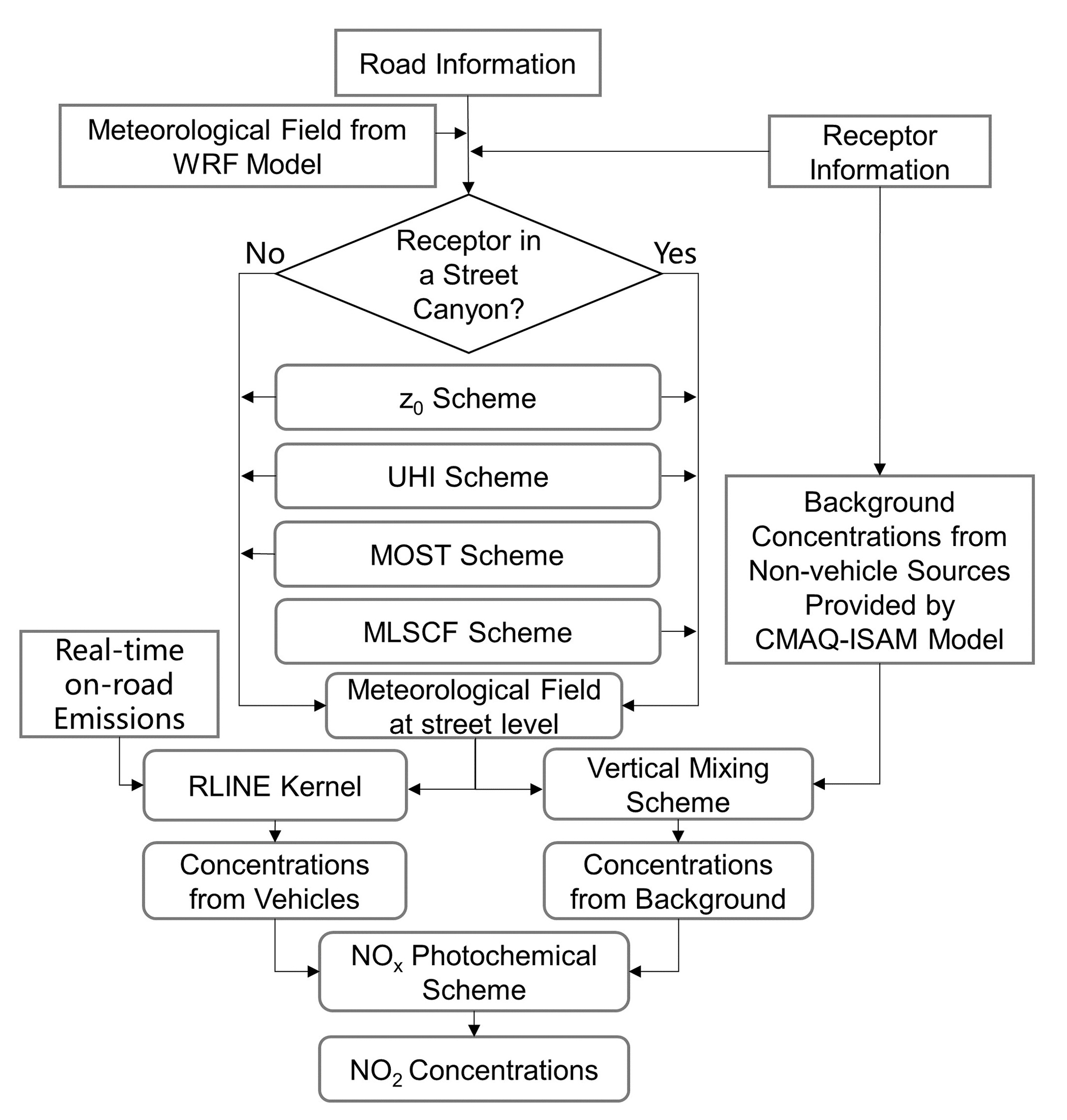
Here, we established the MLSCF scheme based on the R language and modified the code of the RLINE model to add other parameterization schemes with the FORTRAN language. Finally, a multiscale air quality hybrid model was developed to achieve high-resolution NO₂ pollution mapping in urban areas. The framework of CMAQ-RLINE_URBAN is shown in Fig. 1. The hybrid model was established based on the RLINE model, with offline coupling with the gridded meteorological field provided by the WRF model and the pollutant background concentrations from non-vehicle sources provided by the CMAQ model with the Integrated Source Apportionment Method (ISAM), considering the thermodynamic effects caused by the complex underlying surface compositions of the city. Finally, in our hybrid model, an NO₂ pollution map with a high temporal (1 h) and spatial resolution (50 m × 50 m) can be obtained.

Figure 1 The framework of multiscale hybrid model CMAQ-RLINE_URBAN.

RLINE is a Gaussian line source dispersion model developed by Snyder et al. (2013) to predict pollutant concentrations in near-road environments. In the RLINE model, the mobile source is regarded as a finite line source from which the concentration is found by approximating the line as a series of point sources and integrating the contributions of point sources using an efficient numerical integration scheme. The number of points needed for convergence to the proper solution is a function of distance from the source line to the receptor, and each point source is simulated using a Gaussian plume formulation. The RLINE model performs generally comparable results when evaluated with other line source models for on-road traffic emissions dispersion (Snyder et al., 2013; Heist et al., 2013; Chang et al., 2015), and it has been successfully used in many studies to evaluate the impacts from traffic emissions on air quality (Zhai et al., 2016; Valencia et al., 2018; Benavides et al., 2019; Filigrana et al., 2020; X. Zhang et al., 2021).

The simulation for local meteorological conditions in CMAQ-RLINE_URBAN included three steps: estimation for areas above the top of the urban canopy layer (UCL), inside UCL, and inside the street canyon. (1) In this study, the configuration of the WRF model referred to our previous study (Lv et al., 2020). The height of the midpoint in the bottom layer to the ground was set as 22.5 m, which was close to the average height of buildings near street canyons, similar to the settings in the previous study (Benavides et al., 2019). Therefore, the meteorological field simulated by the WRF model was used as the wind field and atmospheric stability at the top of UCL. During the hybrid model running, the meteorological conditions over buildings near each road were obtained separately from the WRF model according to the road location. (2) Then, the surface roughness length (z₀) of each road was estimated based on the surrounding building geometry and used to recalculate the localized meteorological parameters (e.g. Monin–Obukhov length) within UCL according to the algorithm proposed by Benavides et al. (2019) (z₀ scheme). The atmospheric turbulence intensity in urban areas around sunset in the afternoon was obviously enhanced considering the influence of the urban heat island effect based on methods in the AERMOD model (Cimorelli et al., 2005) (UHI scheme). The UHI scheme would affect the turbulent intensity based on the evaluation of the upward surface heat flux and the urban boundary layer height due to convective effects, and then the mixing height, convective velocity scale, surface friction velocity, and Monin–Obhukov length were all recalculated (details in the Supplement Sect. S1). (3) Finally, the wind field within UCL was calculated according to different types of road environments: open terrain and street canyon. The logarithmic wind profile based on Monin–Obhukov similarity theory (MOST) (Foken, 2006) in the original RLINE model was still used when the grid receptor was located in the open terrain (MOST scheme), while the MLSCF parameterization scheme was used for grid receptors within the street canyon to quantitatively characterize the influence of the street canyon geometry and the external wind environment at the top of the roof. The detailed introduction for street canyon geometry and the MLSCF scheme is described in Sect. 2.2.

The real-time vehicle emission inventory used in both regional and local air quality models was based on a street-level on-road vehicle emission (SLOVE) model developed in our previous study (Lv et al., 2020), which was based on the real-time traffic condition data from the map provider AMap (available at https://www.amap.com/, last access: 9 December 2022). The daily averaged NO_x emission from on-road vehicles in Beijing in 2019 was estimated to be 136.0 Mg, of which emissions from heavy-duty vehicles and heavy-duty trucks accounted for 31 % and 34 %, respectively. In our simulation, the concentrations of NO, NO₂, and O₃ excluding contributions from vehicle emissions were used as background concentrations at the roof level, avoiding the double counting in the coupling process. These background concentrations were simulated by the CMAQ-ISAM model, in which the emissions were divided into local mobile and other four emission groups to trace their contributions separately, so the influence of non-local vehicle emissions was considered, and details were presented in our previous study (Lv et al., 2020). The spatial resolution of the innermost domain in both the WRF and the CMAQ model was 1.33 km × 1.33 km. In addition, the influence of atmospheric turbulence and building geometry on the vertical mixing of background concentration was considered (vertical mixing scheme). The ratios of wind speed at surface and roof levels were used as a proxy to calculate the contribution of background concentration over street canyons to the near-ground level (Benavides et al., 2019). In this scheme, the surface wind was from the MLSCF scheme when the grid receptor is located within the street canyon, and otherwise the logarithmic wind profile was used to calculate the wind speed at the specified height, and details were shown in the Supplement Sect. S2. Finally, combined with the vehicle-induced primary NO_x concentration calculated by the RLINE kernel, the high spatial-resolution NO₂ map could be simulated considering the photochemical process of NO_x. In this study, a simplified two-reaction scheme, including the photolysis of NO₂ and the oxidation of NO, was incorporated into the model to characterize the photochemical process of NO_x (details in the Supplement Sect. S3), which has been successfully applied in the SIRANE dispersion model (Soulhac et al., 2017).

2.2 Development for MLSCF scheme

2.2.1 The database of street canyon geometry

We first established a database of street canyon geometry for 15 398 roads in urban areas of Beijing based on the three-dimensional building data obtained from our previous study (Lv et al., 2020) using a geographic information system (GIS). Three typical parameters to represent street canyon geometry were investigated: height ratio ($H_{\mathrm{l}}/H_{\mathrm{r}}$) (H_l is the building height on the left side, while H_r is the building height on the right side), aspect ratio ($H/W$) (H is set to be the average height, and W is the width of the street canyon), and the canyon length-to-height ratio ($L/H$) (L is set to be the length of the street canyon). In this study, the extremely special geometry of canyons was not considered, and the typical street canyons were selected according to the following conditions: (1) the proportion of actual street canyon length (the length of road which the buildings are near) was greater than 0.5; (2) $H/W$ was greater than 0.2; (3) $H_{\mathrm{l}}/H_{\mathrm{r}}$ was between 0.3 and 3.3. Finally, the total number of typical street canyons was 1889, with a total length of 787 km. The spatial distributions of canyon geometry are shown in Fig. S1 in the Supplement. In urban areas of Beijing, street canyons were generally wide, with an average width of 50.3 m, and buildings on both sides were relatively low with a mean of 23.6 m. Most street canyons were obviously located in areas within the 4th ring road. The shallow ($H/W\le \mathrm{0.5}$) canyons and long canyons ($L/H\mathit{>}\mathrm{7}$) dominated, accounting for 54 % and 84 % of the total number of street canyons.

2.2.2 Description of CFD cases

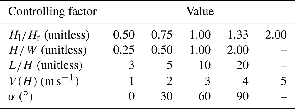
Here, to predict airflow in street canyons comprehensively, CFD simulations were conducted under combinations of different values of controlling factors based on ANSYS FLUENT (v19.2). The controlling factors included the aforementioned three typical parameters to represent canyon geometry, the background wind speed at the height of H (V(H)), and the angle between wind direction and street axis (α) to describe the external wind environment. The selected values of each factor were listed in Table 1, and a total of 1600 (i.e., $\mathrm{5}\times \mathrm{4}\times \mathrm{4}\times \mathrm{5}\times \mathrm{4}$) simulations were implemented.

Table 1 Values of controlling factors used in the simulations.

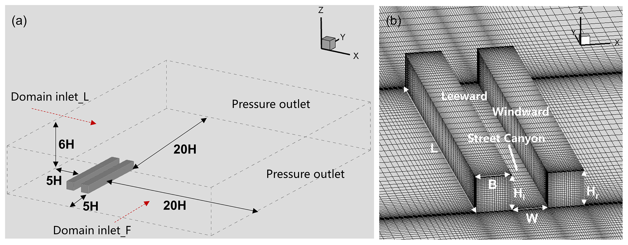
In this study, the computational domain of three-dimensional (3D) full-scale CFD simulations is shown in Fig. 2. The average building height H of the street canyon was always set to 21 m in different simulations, which was similar to the mean street canyon height in Beijing. Other actual sizes of street canyons (e.g., street canyon width W) were calculated according to the ratio of each specific simulation. Distances between urban canopy layer (UCL) boundaries and the domain top, domain inlet, and domain outlet were set as 5H, 5H, and 20H, respectively.

Figure 2 Computational domain (a) and grid arrangement (b) in all CFD test cases.

The turbulence closure schemes for CFD include the Reynolds–Averaged Navier–Stokes (RANS) and the large-eddy simulation (LES), the choice of which depends on the computational cost, the accuracy required, and the purpose of application. The RANS resolves the mean time-averaged properties with all the turbulence motions to be modeled, while LES adopts a spatial filtering operation and consequently resolves large-scale eddies directly and parameterizes small-scale eddies (Zhong et al., 2016). Compared with the LES, the RANS is more easily established and computationally faster (Xie and Castro, 2006). However, the LES can provide a better prediction of airflow than the RANS when handling complex geometries (Dejoan et al., 2010; Santiago et al., 2010). In this study, considering the huge computational burden of a large number of simulations and the relatively simple geometry of street canyons in our modeling, the RANS was selected to characterize the airflow.

Following the CFD guideline (Tominaga et al., 2008; Franke et al., 2011), zero normal gradient conditions or pressure outlet conditions were applied at the domain outlet, and symmetry boundary conditions were adopted at the domain top and two lateral domain boundaries. For near-wall treatment, no-slip wall boundary conditions with standard wall functions were used (FLUENT, 2006). All governing equations for the flow and turbulent quantities were discretized by the finite-volume method with the second-order upwind scheme. The SIMPLE scheme was used for the pressure and velocity coupling. The residual for continuity equation, velocity components, turbulent kinetic energy, and its dissipation rate were all below 10⁻⁵. Meanwhile, the CFD simulation would also stop when the iteration steps exceeded 10 000, due to the large computing cost of so many simulations. In summary, the average iteration steps of a total of 1600 cases were 4443. About 54.6 % of cases met the convergence criteria, and the median residual values of the continuity equation, velocity in the x axis, velocity in the y axis, velocity in the z axis, k, and ε were $\mathrm{1.0}\times {\mathrm{10}}^{-\mathrm{5}}$, $\mathrm{8.5}\times {\mathrm{10}}^{-\mathrm{7}}$, $\mathrm{8.5}\times {\mathrm{10}}^{-\mathrm{7}}$, $\mathrm{4.1}\times {\mathrm{10}}^{-\mathrm{7}}$, $\mathrm{3.4}\times {\mathrm{10}}^{-\mathrm{6}}$, and $\mathrm{5.4}\times {\mathrm{10}}^{-\mathrm{6}}$, respectively, indicating the overall model performance was acceptable. The selected turbulence model and grid arrangement are discussed in Sect. 2.2.3.

At the domain inlet, the power-law velocity profile (Brown et al., 2001), vertical profiles of turbulent kinetic energy k_in, and its dissipation rate ε_in at the domain inlet (Lien and Yee, 2004; K. Zhang et al., 2019), were described below:

$$\begin{array}{}\text{(1)}& {\displaystyle }{U}_{\mathrm{0}}\left(z\right)=U_{\mathrm{ref}}{\left({\displaystyle \frac{z}{H_{\mathrm{ref}}}}\right)}^{\mathit{\alpha }},\text{(2)}& {\displaystyle }{k}_{\mathrm{in}}\left(z\right)={\left(I_{\mathrm{in}}\times U_{\mathrm{0}}\left(z\right)\right)}^{\mathrm{2}},\text{(3)}& {\displaystyle }{\mathit{\epsilon }}_{\mathrm{in}}\left(z\right)={\displaystyle \frac{C_{\mathit{\mu }}^{\mathrm{3}/\mathrm{4}}{k}_{\mathrm{in}}^{\mathrm{3}/\mathrm{2}}}{\mathit{\kappa }z}}.\end{array}$$

Here, U₀(z) stood for the stream-wise velocity at the height z. U_ref represented the reference speed. The reference height H_ref was 21 m. The power-law exponent of α= 0.22 denoted underlying surface roughness above medium-dense urban area (Kikumoto et al., 2017). Turbulence intensity I_in was 0.1, the von Kármán constant κ was 0.41, and C_μ was 0.09.

2.2.3 The CFD validation

In this study, the stream-wise and vertical velocity predicted by CFD within street canyons was compared with wind tunnel data in previous research. For buildings of the cube array model, wind tunnel data from Brown et al. (2001) was used to evaluate the reliability of CFD results by measuring vertical profiles of velocity. In this experiment, the street canyon was perpendicular to the wind direction at the roof level. For long-street models, we predicted horizontal profiles of velocity along the street centerline at the height of z= 0.11H or vertical profiles at some points and then validated CFD simulations using wind tunnel data from Hang et al. (2010). In this validation case, the wind direction at the roof level was parallel to the axis of street canyons. The description and validation results are shown in Figs. S2–S3 and Table S1 in the Supplement, respectively.

We identified the influence of different minimum sizes of hexahedral cells near wall surfaces (fine: 0.1 m; medium: 0.2 m; coarse: 0.5 m) and turbulence models (standard k−ε model and renormalization group (RNG) k−ε model) on the predicted velocity, to evaluate the grid independence and turbulence model accuracy (Fig. S3 in the Supplement). The results indicated that the predictions from the standard k−ε model could match the variations in observed velocity within the street canyon well; these performances were much better than that of the RNG model. In addition, different grid resolutions used in simulations would not obviously affect the predicted results. We finally adopted the standard k−ε model to characterize turbulence, and the minimum size of hexahedral cells near wall surfaces was 0.5 m; an expansion ratio of 1.1 was applied to save the computing cost, and the average mesh number of the total of 80 street canyon models is 1 367 965.

Moreover, the averaged wind speed from CFD in street canyons with different aspect ratios and external wind direction was compared with predictions from other empirical methods used in the SIRANE model (Soulhac et al., 2012) and the MUNICH model (Kim et al., 2018). Similar predictions using different methods also proved the reliability of the CFD simulation in this study (Fig. S4 in the Supplement).

2.2.4 Machine learning

Data-driven methods, such as machine learning and deep learning, are now successful operational geoscientific processing schemes and have co-evolved with data availability over the past decade (Reichstein et al., 2019). Specifically, these models have been used as computationally efficient emulators of explicit mechanism models, to explore uncertainties (Aleksankina et al., 2019) and sensitivities or replace complex gas phase chemistry schemes (Keller and Evans, 2019; Conibear et al., 2021). In addition, meta-models (Fang et al., 2005) such as neural networks and Gaussian process (Beddows et al., 2017) are also used to produce a quick to run model surrogate and show reliable performance. The random forest (RF) model algorithm is an ensemble learning method that generates many decision trees and aggregates their results and has been developed to solve the high variance errors typical of a single decision tree (Breiman, 2001). Multivariate adaptive regression splines (MARS) are a nonparametric and nonlinear regression method, which can be regarded as an extension of the multivariate linear model (Friedman, 1991). RF and MARS are common machine learning methods which run efficiently on large data sets and are relatively robust to outliers and noise. Furthermore, they never require the specification of the underlying data model and the complex parameter tuning, and they can still provide efficient alternatives and generally show a high accuracy in applications for predicting air pollutant concentrations (Hu et al., 2017; Chen et al., 2018; Kamińska, 2019; Geng et al., 2020).

Here, based on the database including 42 880 samples obtained from 1600 CFD simulations, RF and MARS were both used to simulate the wind vector along the x axis (V_x) and the y axis (V_y) at different heights within the street canyon, respectively. The V_x and V_y were the average of all velocities along the x or y axis over the same horizontal profile at a specific height within the street canyons. The input predictor variables included $H/W$, $L/W$, $H_{\mathrm{l}}/H_{\mathrm{r}}$, the grid receptor relative height ($z/H$), and the background wind vector at the height of H along the x axis (${\mathrm{Vbg}}_x=V\left(H\right)\times \sin \mathit{\alpha }$) and the y axis (${\mathrm{Vbg}}_y=V\left(H\right)\times \cos \mathit{\alpha }$). We finally combined the advantages of these two machine learning models and developed the MLSCF scheme to predict wind environment in street canyons and incorporated into the hybrid model, which is discussed in Sect. 3.1.

In the RF model, the number of predictors randomly sampled at each split node in the decision tree (m_try) and the number of trees to grow (NumTrees) are two important hyperparameters that determine the performance of the model. Similarly, in the MARS model, the two important hyperparameters are the total number of terms (nprune) and the maximum number of interactions (degree). By comparing the mean squared error (MSE) for testing datasets across models with candidate parameter combinations, we set m_try and NumTrees as 6 and 200 in RF, respectively, and nprune and degree as 23 and 3 in MARS, respectively. Additionally, the 10-fold cross-validation (CV) repeated 10 times was considered to evaluate the prediction performance of our models. The total dataset was randomly divided into 10 subsets, where 9 subsets was used to train the model and another was applied for validation. The fitted coefficients of MARS are shown in Tables S2–S3 in the Supplement.

In order to identify the sensitivity and response relationship between prediction variables and results in the RF model, we used the MSE for out-of-bag (OOB) estimates to evaluate the relative importance of each feature to V_x and V_y, by randomly replacing the value of a single prediction variable one by one (Liaw and Wiener, 2002). Higher values of increase in MSE indicated that the predictor was more important. In addition, partial dependence plots (PDPs) were applied to establish the response relationship between the change in a single predictive variable and the predicted results, considering the average influence of other variables (Greenwell, 2017).

2.3 Configuration of CMAQ-RLINE_URBAN

The near-ground NO₂ concentrations were simulated from 1 to 31 August 2019 when the average of daily high temperatures was higher than 30 ^∘C and sunlight duration was longer than 13 h, leading to strong photochemical reactions. The simulation domain for the hybrid model covered the core urban areas within and surrounding the 5th ring road, shown in Fig. 3. The receptors included both grid receptors and monitor receptors. The grid receptors were set at a spatial resolution of 50 m × 50 m, and the height above the ground was 1.5 m, which was equivalent to the height of human breathing. We used data from 10 observation stations (monitor receptors) located in the normal urban environment and 5 near-road monitoring sites for validation (Beijing Ecological Environment Monitoring Center, available at http://zx.bjmemc.com.cn/, last access: 9 December 2022) (DSH, NSH, QM, XZM, and YDM) in the simulation domain (Fig. 3), which were 10 and 3 m above the ground, respectively. The QM and XZM sites were located in shallow street canyons, and details of the morphometry of near-road measurement sites are shown in Table S4 in the Supplement.

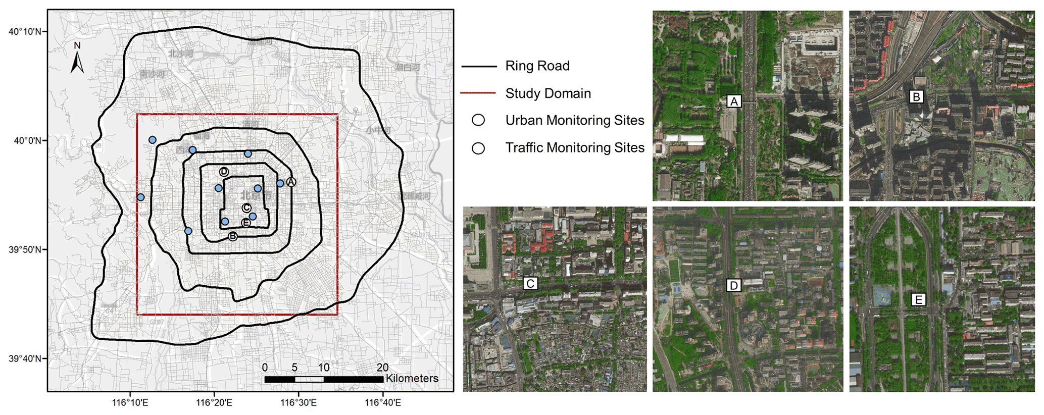
Figure 3 Study domain (© OpenStreetMap contributors 2020. Distributed under the Open Data Commons Open Database License (ODbL) v1.0) and location of monitoring sites (© Microsoft). A: DSH; B: NSH; C: QM; D: XZM; E: YDM.

In general, compared to the RLINE model, CMAQ-RLINE_URBAN has the following improvements:

• a.

  The gridded meteorological parameters provided by the WRF model were used.

• b.

  Gridded non-vehicle-related concentrations provided by the CMAQ-ISAM model were used as background concentrations.

• c.

  A simple NO_x photochemical scheme was incorporated to simulate NO₂ concentrations.

• d.

  Thermodynamic effects caused by the special underlying surface structures of the city were considered, including UHI effects, the influence of local buildings on turbulence intensity, and vertical mixing of background concentrations.

• e.

  A newly developed MLSCF scheme was applied to predict the wind environment in street canyons.

In our simulation, the model configurations in the base scenario CMAQ-RLINE_URBAN included all (a)–(e) schemes, and the other two control scenarios were set to investigate the sensitivity of urban schemes to predictions, where all input data were set to be the same. The scenario CMAQ-RLINE only including (a)–(c) schemes was set to analyze the impacts of urban thermodynamic schemes, and the scenario CMAQ-RLINE_URBAN_nc including (a)–(d) schemes was set to identify the impacts of the MLSCF scheme. Although the wind environment for each road at the top of the canyon was provided by the WRF model in all scenarios, the calculation of wind profiles within the street canyon was different. It was estimated based on the MOST theory in the CMAQ-RLINE and CMAQ-RLINE_URBAN_nc rather than that from MLSCF in the CMAQ-RLINE_URBAN.

3 Results

3.1 Fitting results of machine learning

In this study, the 10-fold cross-validation (CV) repeated 10 times was considered to evaluate the prediction performances of RF and MARS models. As shown in Figs. 4 and S5, both models performed with acceptable robustness in CV, indicating that neither the RF nor the MARS model overfitted the data. In general, the performances of both models in predicting V_y was better than that for V_x of which the absolute value was relatively small, especially for the MARS model. Since V_x was responsible for the formation of the vortex within street canyons and affected by multiple factors, it was more difficult to simulate. The averages of mean absolute error (MAE), root mean square error (RMSE), and correlation coefficient (R) in the CV of the RF model were 0.04, 0.02 m s⁻¹, and 0.99, respectively, for V_x and 0.05, 0.03 m s⁻¹, and 0.99, respectively, for V_y. Although the average of the relative error (RE) was a little high (42.5 % and 43 %), particularly when the predicted wind speed was low, the median RE was relatively low with 9.8 % and 2.7 %, respectively, indicating an acceptable performance. Compared with the advanced nonlinear RF algorithm, the MARS model did not perform very well, especially when the absolute value of V_x was greater than 1 m s⁻¹ and V_y was less than 3 m s⁻¹. However, when the predicted wind speed by machine learning methods was compared with observations from wind tunnel experiments, we found that the performance of the MARS model was obviously better than that of RF model in one of the validation cases (see Fig. 5). The decision tree model like RF failed to respond to the parts beyond the range of prediction variables (Vbg_y= 17 m s⁻¹ ≫ 5 m s⁻¹), while the more reasonable predictions can be obtained by the MARS model, which essentially used a piecewise linear function. Therefore, the MLSCF scheme was established based on a method to combine the advantages of each model. The RF model was used when the input value was within the range of predictors shown in Table 1; otherwise the predictions from the MARS model were used.

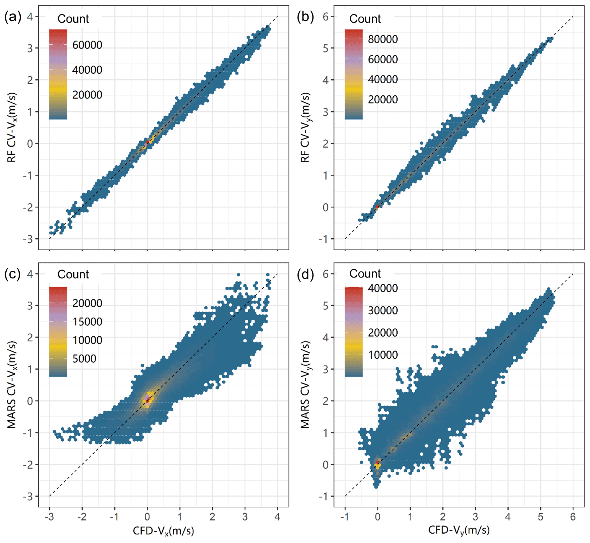
Figure 4 Cross-validations of machine learning models for V_x (a, c) and V_y (b, d): (a–b) RF model; (c–d) MARS model.

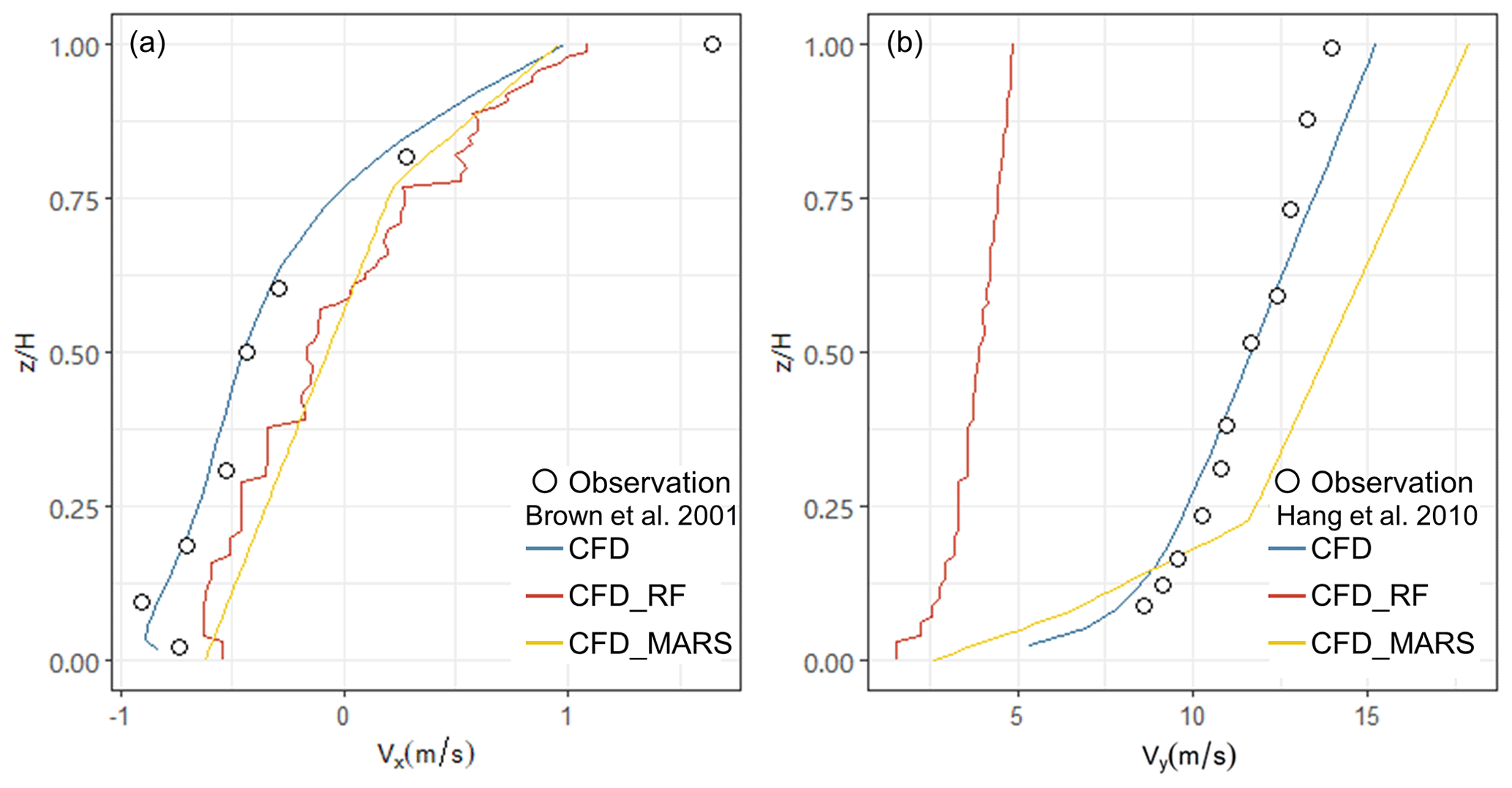
Figure 5 Performances of machine learning on the velocity profile in wind tunnel experiments. The street canyon was perpendicular (a) or parallel (b) to the wind direction at the roof level in different experiments. The detailed description of each experiment was introduced in Sect. 2.2.3.

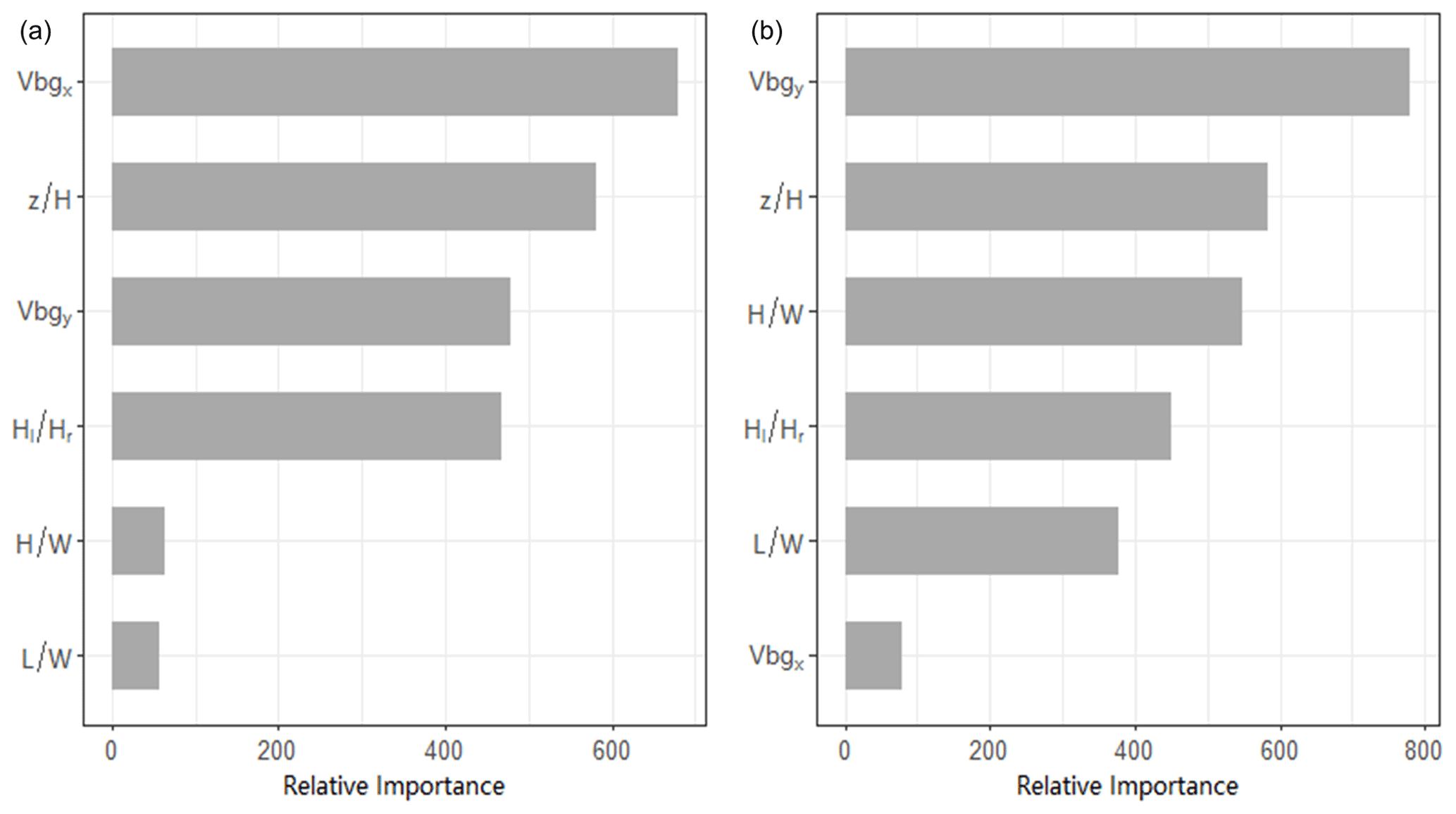
In addition, the importance of each predictor variable in the RF model was investigated to explain their impacts on predictions. As shown in Fig. 6, the background wind speeds on the x and y axes played vital roles in predictions of V_x and V_y, respectively, followed by the relative height ($z/H$). Among the geometric parameters of the street canyon, the impact of $L/W$ was the lowest. Since V_x was the main driving force for the formation of vortices in street canyons, it was more affected by the geometry of street canyons, especially $H_{\mathrm{l}}/H_{\mathrm{r}}$, compared to V_y. This feature importance ranking was basically consistent with the conclusion in a previous study (Fu et al., 2017). Figure S6 in the Supplement shows the PDPs of each predictor variable in the RF model for V_x and V_y. As $z/H$ grew, V_x and V_y showed linear and logarithmic increase patterns, respectively. Moreover, the resistant effect of windward buildings on wind speed enhanced with increasing $H_{\mathrm{l}}/H_{\mathrm{r}}$, resulting in a significant decrease in V_x particularly when $H_{\mathrm{l}}/H_{\mathrm{r}}$ was lower than 1.25. The relationship between predictors and results in the model was consistent with the actual mechanism, indicating our model could provide an accurate description of the wind field in the street canyon.

Figure 6 Variable importance ranking in the RF model for (a) V_x and (b) V_y.

3.2 Impacts of MLSCF on simulations in street canyons

We compared the differences between monthly mean wind profile in different street canyons including QM (shallow canyon: $H/W=\mathrm{0.22}$), XZM (shallow canyon: $H/W=\mathrm{0.35}$), SZJ (standard canyon: $H/W=\mathrm{1}$), and JTDL (deep canyon: $H/W=\mathrm{1.93}$), calculated by the default logarithmic function based on MOST in the original RLINE model (Foken, 2006) and the MLSCF scheme developed in this study. As shown in Fig. 7a–d, the wind profile estimated by MOST showed a logarithmic change at the height above displacement height (d_h) with a decrease to 0 at d_h and remained constant below d_h (the d_h is calculated by multiplying surface roughness length (z₀) times a factor which is recommended to be set as 5). Compared with the MOST, the simulated wind speeds near the ground and at the top of canyons were generally lower based on the MLSCF scheme in shallow and standard street canyons. In the deep street canyon, the significant reduction in ventilation volume led to the mean wind speed simulated by the MLSCF scheme being much lower than that of MOST at all heights. Although the aspect ratios of the street canyon located in QM and XZM were similar, their orientations were quite different, resulting in significant differences under prevailing external winds in different directions. Since prevailing northerly and southerly winds were observed in Beijing during the study period, the resistance effect of the buildings on both sides of the east–west street canyon located in QM was more obvious.

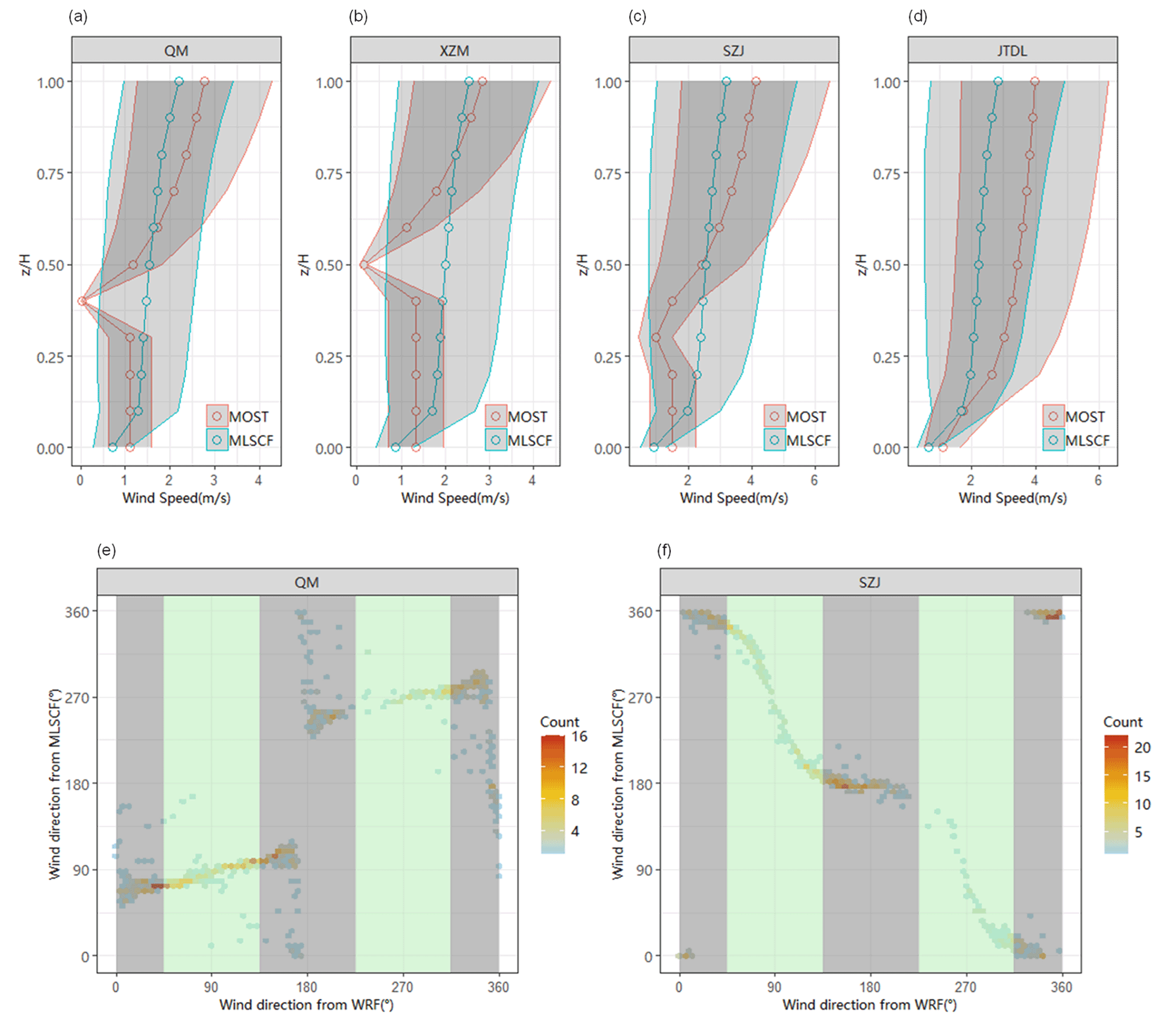
Figure 7 Influence of MLSCF on wind environment in the street canyon. Monthly averaged vertical profile of wind speed from the MOST and MLSCF methods in different street canyons: (a) QM ($H/W=$ 0.22); (b) XZM ($H/W=$ 0.35); (c) SZJ ($H/W=$ 1); (b) JTDL ($H/W=$ 1.93). The gray shading represents the standard deviation in results of all hours. Hourly wind direction from the WRF model (at roof level) and the MLSCF method (at ground level) in different street canyons: (e) QM ($H/W=$ 0.22); (f) SZJ ($H/W=$ 1). As the gray and green shading shown, the background wind over the street canyon provided by the WRF model was divided into four main directions: east, west, south, and north.

We also investigated the impacts of the MLSCF hourly wind direction at the bottom (z=3 m) of different street canyons by comparing the roof-level predictions from the WRF model (see Fig. 7e–f). In a shallow street canyon like QM, the simulated wind direction at the bottom was consistent with the background on the whole, with R reaching 0.8. When the background wind direction was less than 180^∘, the averaged wind direction at the bottom simulated by MLSCF was 91.8^∘, which was basically consistent with the angle between the street and the south direction (84.5^∘). When the background wind direction was greater than 180^∘, the average wind direction predicted by MLSCF (257.4^∘) was similar to that in the opposite direction of the street (264.5^∘), which was in line with the theory proposed by Soulhac et al. (2008) that the average wind direction in street canyons was assumed to be consistent with the (opposite) orientation of the street. While in the deep street canyon of SZJ, when the external wind perpendicularly blew to the street, the wind direction at the bottom was completely opposite to that at the top due to the formation of vortex, with R reaching −0.97. In conclusion, compared with the traditional MOST method, the newly developed MLSCF scheme could simulate the influence of the external wind environment and geometry on the wind field well inside the street canyon.

As shown in Fig. 8, the impacts of the MLSCF scheme on simulated NO₂ concentration were identified by the differences between the CMAQ-RLINE_URBAN and CMAQ-RLINE_URBAN_nc scenarios during a clean day (24 August). When the atmosphere was stable at night, in street canyons with a large aspect ratio, the wind direction at the bottom changed to the opposite of that at the top. Combined with the decreased wind speed affected by the MLSCF scheme, the NO₂ concentrations at upwind grid receptors increased by up to 80 µg m⁻³. Meanwhile, the changes in wind direction would also decrease the concentrations at downwind grid receptors by up to 20 µg m⁻³. For example, in the SZJ standard canyon, the background wind direction over the street was 79^∘ (easterly), and the wind direction at the bottom changed to 291^∘ affected by the MLSCF scheme (westerly). Therefore, the upwind NO₂ concentrations increased, and the location of peak NO₂ concentration shifted to the windward direction. Since the changes in NO₂ concentrations were also influenced by the local on-road emissions, the increase was only up to 2.1 µg m⁻³ in SZJ street, where the traffic flow and vehicle emissions were low at night. However, a little influence was observed during the day in the convective boundary layer. During this period, although the wind direction at the bottom did not change obviously due to the parallel background wind in SZJ street, the increased surface wind speed was beneficial for the dispersion, resulting in the decreased concentration in grid receptors within both sides of the street canyon. In summary, the MLSCF scheme enabled the characterization of the concentration distribution in street canyons.

Figure 8 Differences in NO₂ concentrations at the height of 1.5 m impacted by the MLSCF scheme (a, c) over the study domain (CMAQ-RLINE_URBAN – CMAQ-RLINE_URBAN_nc) (© Microsoft) and (b, d) near SZJ in 24 August 2019 at 00:00–01:00 (a, b) and 10:00–11:00 (c, d).

3.3 Performance of near-road simulations from different models

The performances in predicting NO₂ concentrations at all monitor receptors from different models were first compared, including the CMAQ-RLINE_URBAN, CMAQ-RLINE, and CMAQ models. The mean bias (MB), RMSE, normalized mean bias (NMB), normalized mean gross error (NMGE), the fraction of predictions within a factor of 2 (FAC2), the index of agreement (IOA), and R between simulations and observations were all selected as statistical indicators for the evaluation (Table 2). In general, the performance of CMAQ-RLINE_URBAN was the best at all urban sites. Compared to the CMAQ model, the averaged MB and NMB at urban sites in the hybrid model decreased from 8 to 1.3 µg m⁻³ and 27 % to 4 %, respectively.

Table 2 Model performances under different scenarios.

MB: mean bias; RMSE: root mean squared error; NMB: normalized mean bias; NMGE: normalized mean gross error; FAC2: fraction of predictions within a factor of 2; IOA: index of agreement; R: correlation coefficient.

Diurnal variations in observed and predicted hourly averaged NO₂ concentrations at near-road sites from different models were mainly compared and shown in Fig. 9. The comparison of hourly and daily averaged concentrations is shown in Fig. 10. Overall, CMAQ-RLINE_URBAN performed best with the smallest deviations. By comparing the performances of the CMAQ and CMAQ-RLINE scenarios, we found the direct coupling between the CMAQ and RLINE models could reproduce the high NO₂ concentrations at near-road sites in the daytime and significantly improve the underestimation of near-source concentrations due to grid dilution of emissions in the CMAQ model. The averaged MB and NMB at all sites changed from −10 to 25.6 µg m⁻³ and from −20 % to 51 %, respectively. However, a significant overestimation was found in CMAQ-RLINE at night (00:00–06:00; all times in this paper are given in local time) and around sunset in the afternoon (16:00–23:00), of which the peak could exceed the observed concentrations by more than 1-fold. This overestimation was reduced in the CMAQ-RLINE_URBAN, where the urban thermodynamic schemes were implemented. The averaged MB and NMB decreased to 6.3 µg m⁻³ and 12 %, respectively, for the following reasons: (1) the increased surface roughness length slightly enhanced local turbulence intensity near roads; (2) the UHI scheme enhanced the intensity of atmospheric turbulence in urban areas before and after sunset in the afternoon; (3) the effect of turbulence intensity on the local vertical mixing of background concentrations was considered, significantly reducing the mixing ratio of concentrations over UCL and near the ground at nights in the stable boundary layer (Fig. S7 in the Supplement), which was probably the main driving force of decreased predictions in the hybrid model (Benavides et al., 2019). However, CMAQ-RLINE_URBAN slightly overestimated the nighttime NO₂ concentration of all observation stations except the DSH, which was probably caused by overestimations of background concentrations from CMAQ-ISAM and vehicle emissions.

Figure 9 Diurnal variations in observed and predicted hourly averaged NO₂ concentrations from different models at near-road monitoring sites: (a) DSH; (b) NSH; (c) QM; (d) XZM; (e) YDM.

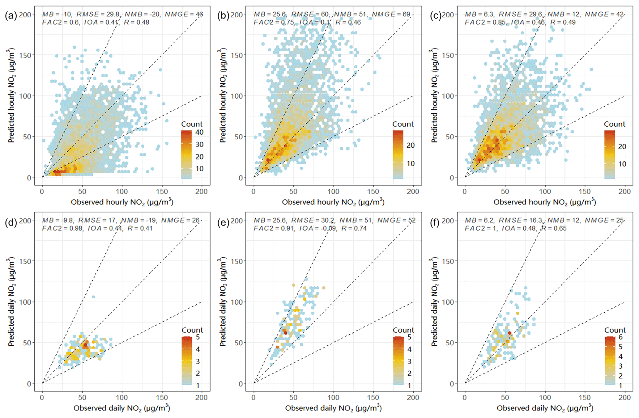
Figure 10 Observed and predicted hourly (a–c) or daily averaged (d–f) NO₂ concentrations from different models at near-road sites: (a, d) the CMAQ model; (b, e) the CMAQ-RLINE model; (c, f) the CMAQ-RLINE_URBAN model.

The accuracy of model performances at each traffic site showed a small difference affected by the variations in the traffic flow and emissions of nearby roads as well as the geometry of surrounding buildings and street canyons. At the DSH and NSH sites, which were adjacent to ring roads as the main urban freight corridors with a high traffic flow including a large proportion of trucks, the high NO_x emissions led to the highest roadside NO₂ observations among all sites. The CMAQ model would significantly underestimate the high NO₂ concentration at sites nearby ring roads, with MB and NMB lower than −15 µg m⁻³ and −28 % (Table S5 in the Supplement), respectively, which was improved using CMAQ-RLINE_URBAN. However, the hybrid model produced a minor overestimation at the NSH site, since the monitor was actually positioned in the road centerline but assumed to be located downwind in the model, resulting in a relatively large systematic error (Snyder et al., 2013). In total, CMAQ-RLINE_URBAN performed best among all models, especially improving the estimation of NO₂ concentrations near roads by the original regional model.

Additionally, Fig. S8 in the Supplement shows the comparison between simulated and observed roadside hourly and daily maximum 8 h average O₃ concentrations by different models, and their diurnal variations are shown in Fig. S9. Generally, the hybrid model significantly improved the overestimation of daytime O₃ concentrations by the CMAQ model when considering the titration effect of high NO concentration near roads on O₃. In the hybrid model, the peak time was delayed to about 15:00, which was closer to the observation, but still 1–2 h earlier than the actual time, which may be related to the uncertainty in the NO₂ photolysis rate.

3.4 Spatial distribution characteristics of simulated concentrations

We investigated the differences between the spatial distribution of the monthly averaged NO₂ concentration simulated by the CMAQ and CMAQ-RLINE_URBAN models, as shown in Fig. 11. Since the urban thermodynamic schemes were considered in the hybrid model, the overestimation of most urban environmental grid receptors by the CMAQ model was relieved. Within the 4th ring road and its surrounding areas, the mean concentration of NO₂ from CMAQ-RLINE_URBAN was 30.1 µg m⁻³, lower than that from the CMAQ model (39.5 µg m⁻³). The overall spatial distribution characteristics of NO₂ predictions from both models showed that the concentrations in south regions were high due to the pollution transport from Hebei province (An et al., 2019). However, near-road hotspots for the NO₂ pollution were identified in the hybrid model where the spatial resolution of results increased to 50 m × 50 m. The NO₂ concentrations nearby ring roads with high traffic flow and emissions were up to 120 µg m⁻³, much higher than the maximum prediction from the CMAQ model (52.4 µg m⁻³). In addition, the simulated near-road concentrations from the hybrid model during traffic peak hours (18:00–19:00) were significantly higher than those at noon (12:00–13:00), while there were few changes in results from the CMAQ model (Fig. S10 in the Supplement).

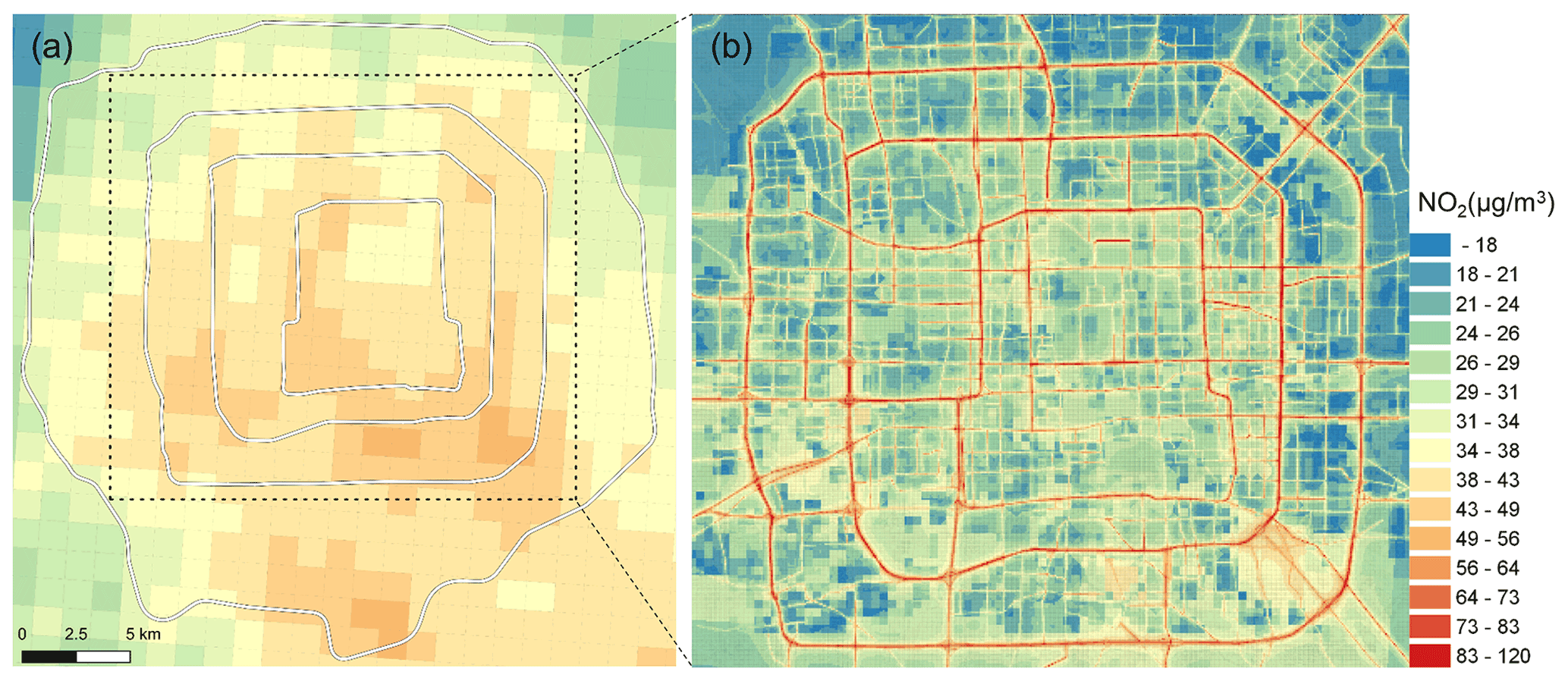
Figure 11 Spatial distribution of monthly averaged NO₂ concentrations from (a) the CMAQ model and (b) the CMAQ-RLINE_URBAN model. (© OpenStreetMap contributors 2020. Distributed under the Open Data Commons Open Database License (ODbL) v1.0.)

The NO₂ concentrations estimated by CMAQ-RLINE_URBAN at all grid receptor followed a two-mode Gaussian distribution (Fig. S11 in the Supplement), which was similar to Zhang's results (Y. Zhang et al., 2021). The NO₂ concentrations as a result of vehicle emissions were further calculated by the differences between the total and background concentrations. In general, the vehicle-induced NO₂ concentrations in urban areas were 11.8 µg m⁻³, accounting for 39 % of the total concentrations, which was similar to the predicted contribution from the CMAQ-ISAM model (42.5 %).

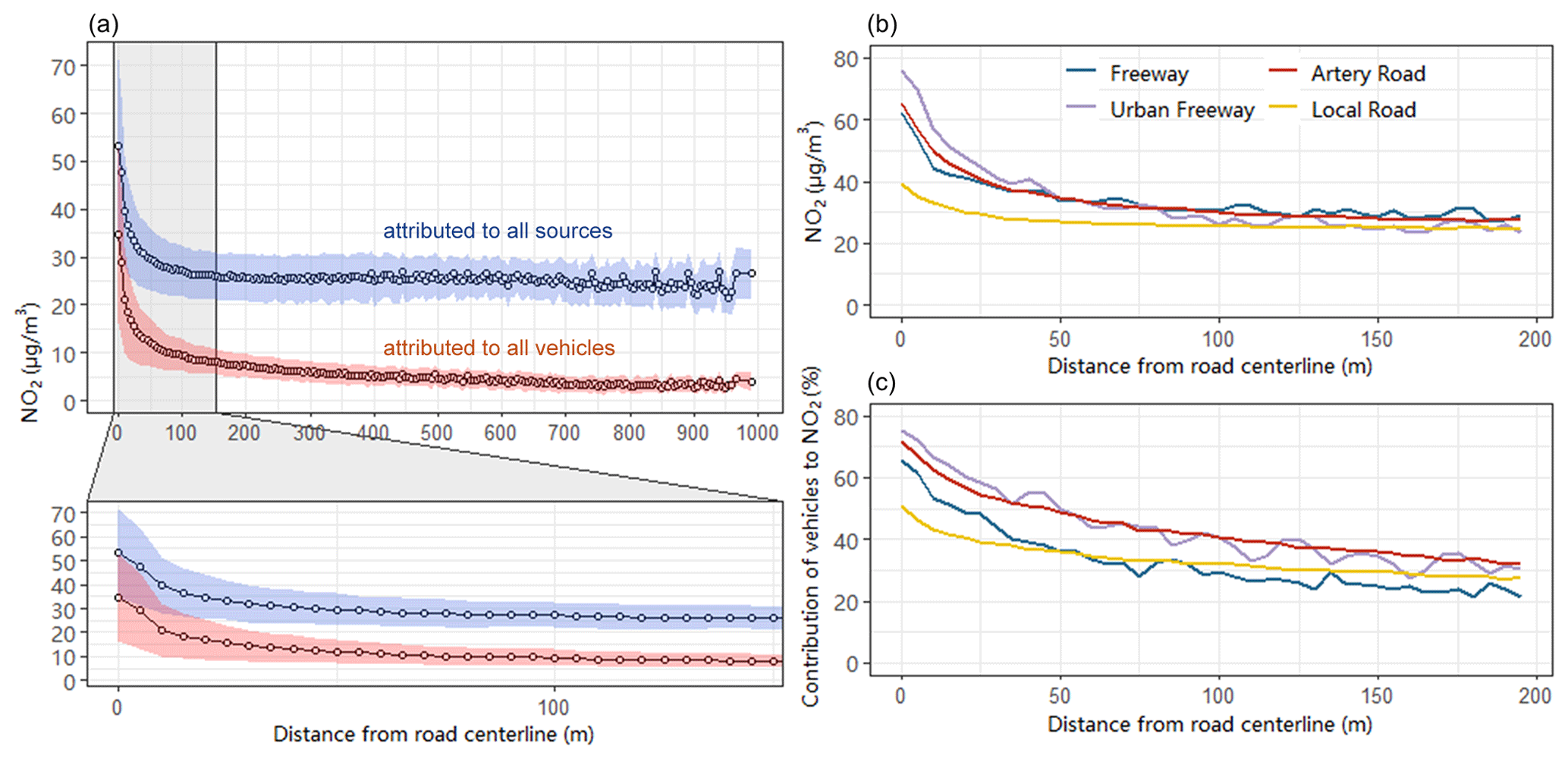
Figure 12 Monthly averaged NO₂ concentrations attributed to all emission sources or vehicles with a distance from the receptor to its nearest road centerline. (a) NO₂ attributed to all emission sources near all roads. (b) NO₂ attributed to all emission sources near different road types. (c) Relative contribution of vehicles to NO₂ near different road types. The shaded area in (a) represents the standard deviation in the results of all receptors.

Figure 12 shows the changes in NO₂ concentrations simulated by the hybrid model with distance from the grid receptors to its nearest road centerline. The concentrations at grid receptors within 200 m from the road were significantly affected by vehicle emissions. Within 50 m around the road, as the distance from grid receptors to the road centerline gradually increased, the NO₂ concentrations decreased exponentially. The total NO₂ concentrations decreased from 53.1 to 30 µg m⁻³, and the vehicle-induced concentrations also dropped from 34.7 to 12.6 µg m⁻³. The concentrations near roads with different types were highly dependent on the emission intensity. The NO₂ concentration was highest in the center of the urban freeway, which was 76 µg m⁻³ and about 1.9 times higher than that on local roads. The relative contribution of vehicle emissions to NO₂ concentration reached up to 75.3 % on urban freeways as well as 71.9 % and 65.5 % on artery roads and freeways but only 51.1 % on local roads. It was worth noting that although the NO₂ concentrations at grid receptors far from the road on highways were slightly higher than those on other road types, the contribution of vehicle emissions was the lowest. This was because the NO_x emission intensity of freeways was as high as that on artery roads, but the density and height of buildings around freeways were usually low, resulting in a high vertical flux of background concentrations from the top of UCL to the ground. In conclusion, the results from the hybrid model accurately reflected not only the impacts of local on-road emissions but also the pollution characteristics affected by non-vehicle sources at the regional scale.

4 Conclusion and discussions

In this study, we developed a hybrid model CMAQ-RLINE_URBAN to quantitatively analyze the effects of vehicle emissions on urban roadside NO₂ concentrations at a high spatial resolution of 50 m × 50 m. The main conclusions of this study are as follows.

The developed MLSCF scheme revealed that, affected by the geometry of buildings on both sides of the road, the wind environment in the street canyon was sometimes quite different from that in the environmental background. In deep street canyons, the wind speed at the bottom decreased obviously due to the resistant effect of buildings, and the directions of horizontal flow at the bottom and top of the canyon were completely opposite due to the formation of a vortex. The application of the MLSCF scheme in the hybrid model led to increased NO₂ concentrations at upwind grid receptors within deep street canyons due to changes in the wind environment. However, the influence of the turbulence induced by street canyon effects on the mixing of air pollution was not considered, which we will make an effort to do in the future.

The comparison between observations and predictions showed that the hybrid model significantly improved the underestimation of near-source concentrations due to grid dilution of emissions in the CMAQ model. The implementation of the urban thermodynamic schemes in the hybrid model also relieved the overestimation in nighttime NO₂ concentrations from CMAQ directly coupled with the RLINE model. The predictions from the CMAQ-RLINE_URBAN model could accurately reflect not only the impact of local road emissions but also the pollution characteristics of non-vehicle sources at a regional level. It revealed that in summer, the average contribution of vehicle emission to NO₂ concentrations in urban areas of Beijing was 11.8 µg m⁻³, and the relative contribution accounted for approximately 39 %. Moreover, the vehicle-induced NO₂ pollution increased significantly with the decreased distance to the road centerline, especially reaching 76 µg m⁻³ (75 %) on urban freeways.

On the basis of this study, the following perspectives are proposed for future research. (1) At present, the execution time during 1 h running CMAQ-RLINE_URBAN over the urban domain was about 3.9 h on average, which reached 4.8 h at night due to the difficulty of convergence under conditions of high atmospheric stability. Therefore, considering the running cost, the grid resolution of the area in Beijing of the 5th ring road and its surroundings can reach 50 m × 50 m. We will make efforts to develop a parallel computing method to reduce the computing time, in order to improve the grid resolution of a relatively large-scale simulation. (2) In our study, a simplified two-reaction scheme was incorporated into the model to characterize the photochemical process of NO_x, since it performed similar predictions and less computational time compared with those of the complicated CB05 gas phase chemical mechanism (Kim et al., 2018). However, another study pointed out that the impact of nonlinear O₃–NO_x–VOC chemistry on NO₂ concentrations in the deep canyon was non-negligible (Zhong et al., 2017). The influence of different chemistry schemes on near-road simulation will be investigated in the future. (3) It was suggested that the long-term site observation of wind environment and pollutant concentrations in various street canyons should be compared with modeling results, especially in deep street canyons with a large aspect ratio. The navigation monitoring technology would be applied in the model verification, which can carry out large-scale observation of concentrations along streets. (4) Here, we considered the dynamic impact of idealized building structures on the wind environment in street canyons. However, there are many other influencing factors, such as building layout and arrangement, roof shape, green vegetation, and thermodynamic effects, which we suggest should be considered in future studies. (5) In this study, we mainly focused on the NO₂ concentrations. In fact, the concentration of particulate matter, especially UFP, will also have an obvious peak near the road centerline. In the future, the process of physical and chemical changes in particulate matter near the vehicle exhaust outlet should be further investigated. (6) The high-resolution NO₂ concentration map will be beneficial for the estimation of human health risks induced by air pollution at the street level in future research.