the Creative Commons Attribution 4.0 License.
the Creative Commons Attribution 4.0 License.
 | 12 Dec 2022
Atmospheric methane isotopes identify inventory knowledge gaps in the Surat Basin, Australia, coal seam gas and agricultural regions
Bryce F. J. Kelly
Xinyi Lu
Stephen J. Harris
Bruno G. Neininger
Jorg M. Hacker
Stefan Schwietzke
Rebecca E. Fisher
James L. France
Euan G. Nisbet
David Lowry
Carina van der Veen
Malika Menoud
Thomas Röckmann
In-flight measurements of atmospheric methane (CH4(a)) and mass balance flux quantification studies can assist with verification and improvement in the UNFCCC National Inventory reported CH4 emissions. In the Surat Basin gas fields, Queensland, Australia, coal seam gas (CSG) production and cattle farming are two of the major sources of CH4 emissions into the atmosphere. Because of the rapid mixing of adjacent plumes within the convective boundary layer, spatially attributing CH4(a) mole fraction readings to one or more emission sources is difficult.
The primary aims of this study were to use the CH4(a) isotopic composition (δ13C) of in-flight atmospheric air (IFAA) samples to assess where the bottom–up (BU) inventory developed specifically for the region was well characterised and to identify gaps in the BU inventory (missing sources or over- and underestimated source categories). Secondary aims were to investigate whether IFAA samples collected downwind of predominantly similar inventory sources were useable for characterising the isotopic signature of CH4 sources (δ13C) and to identify mitigation opportunities.
IFAA samples were collected between 100–350 m above ground level (m a.g.l.) over a 2-week period in September 2018. For each IFAA sample the 2 h back-trajectory footprint area was determined using the NOAA HYSPLIT atmospheric trajectory modelling application. IFAA samples were gathered into sets, where the 2 h upwind BU inventory had > 50 % attributable to a single predominant CH4 source (CSG, grazing cattle, or cattle feedlots). Keeling models were globally fitted to these sets using multiple regression with shared parameters (background-air CH4(b) and δ13C).
For IFAA samples collected from 250–350 m a.g.l. altitude, the best-fit δ13C signatures compare well with the ground observation: CSG δ13C of −55.4 ‰ (confidence interval (CI) 95 % ± 13.7 ‰) versus δ13C of −56.7 ‰ to −45.6 ‰; grazing cattle δ13C of −60.5 ‰ (CI 95 % ± 15.6 ‰) versus −61.7 ‰ to −57.5 ‰. For cattle feedlots, the derived δ13C (−69.6 ‰, CI 95 % ± 22.6 ‰), was isotopically lighter than the ground-based study (δ13C from −65.2 ‰ to −60.3 ‰) but within agreement given the large uncertainty for this source. For IFAA samples collected between 100–200 m a.g.l. the δ13C signature for the CSG set (−65.4 ‰, CI 95 % ± 13.3 ‰) was isotopically lighter than expected, suggesting a BU inventory knowledge gap or the need to extend the population statistics for CSG δ13C signatures. For the 100–200 m a.g.l. set collected over grazing cattle districts the δ13C signature (−53.8 ‰, CI 95 % ± 17.4 ‰) was heavier than expected from the BU inventory. An isotopically light set had a low δ13C signature of −80.2 ‰ (CI 95 % ± 4.7 ‰). A CH4 source with this low δ13C signature has not been incorporated into existing BU inventories for the region. Possible sources include termites and CSG brine ponds. If the excess emissions are from the brine ponds, they can potentially be mitigated. It is concluded that in-flight atmospheric δ13C measurements used in conjunction with endmember mixing modelling of CH4 sources are powerful tools for BU inventory verification.
- Article
(15460 KB) - Full-text XML
- BibTeX
- EndNote


There is considerable international interest in mapping and mitigating sources of methane (CH4) because it is a potent greenhouse gas. This is reflected by the fact that over 100 countries signed the international CH4 pledge launched at COP26 in November 2021, which aims to strengthen support for CH4 emission reduction initiatives (https://www.globalmethanepledge.org/, last access: 8 December 2022). Currently there are plans to expand coal seam gas (CSG; refer to Appendix A, Sect. A1, for a listing of abbreviations) and shale gas productions throughout many regions of Australia (Australian Government, 2021); thus it is critical to understand how this expansion will contribute to regional, national, and global emissions. We also need to improve our knowledge of greenhouse gas emissions from agricultural districts. This study uses CH4 carbon isotopic composition (δ13C) to gain additional insights into CSG, coal mining, and agricultural contributions to regional and global atmospheric emissions. We also demonstrate how atmospheric isotope studies can identify mitigation opportunities.
The southeast portion of the Surat Basin, Queensland, Australia is an area of approximately 200 km by 200 km, where there are over 4000 producing CSG wells, active and inactive open-pit coal mines, piggeries, and millions of beef cattle in feedlots (called feedlots below) and grazing throughout the mixed agricultural districts. The study area covers approximately 0.5 % of Australia yet produces 3 %–4 % of Australia's CH4 emissions (Australian Government, 2020a, b; Neininger et al., 2021). Other CH4 sources close to CSG production in the Surat Basin include domestic wood heaters, landfills, wastewater treatment plants, and natural seeps from the Condamine River. The rapid expansion of CSG in the southeastern region of the Surat Basin has resulted in considerable research interest in quantifying the emissions from the CSG sector. A review of all past ground-based CH4 surveys in the region is presented in Lu et al. (2021).
The Australian Government has developed its own methods for estimating emissions from CSG facilities (Australian Government, 2020b; Neininger et al., 2021). Because of Australia's unique climate and farming practices there are many locally approved emission factors for agricultural sources and methods for determining regional emissions (Australian Government, 2020b; EFDB, 2006; IPCC, 2006, 2019). Inventories prepared using the national and IPCC emission factors are commonly called bottom–up (BU) emission estimates (Neininger et al., 2021), and an emission factor is a coefficient that quantifies the emissions or removals of a gas per unit of activity (IPCC, 2006, 2019). To support the CH4 studies in the Surat Basin a BU inventory was calculated for the region using the methods outlined in Australia's 2018 National Inventory submission to the UNFCCC (Australian Government, 2020a). The comprehensive details about that inventory and the data sets used are discussed at length in Neininger et al. (2021). In the past decade there has been increased use of top–down (TD) airborne and satellite measurements to verify BU inventories (Barkley et al., 2017; Gorchov Negron et al., 2020; Karion et al., 2013, 2015; Neininger et al., 2021; Peischl et al., 2015, 2016, 2018; Pétron et al., 2014; Schwietzke et al., 2017; Turner et al., 2015; Yacovitch et al., 2018; Zhang et al., 2020, 2021). Previous studies have shown that it is not uncommon to find a large difference between BU inventory versus TD estimates of emissions (Kirschke et al., 2013; Desjardins et al., 2018; Saunois et al., 2020). Much of this uncertainty is due to the quality and resolution of the base data sets used for calculating the emissions (Han et al., 2020; Verhulst et al., 2017).
In 2018 and 2019 CH4 emissions from many facilities were mapped using a car-mounted Los Gatos Research ultraportable greenhouse gas analyser (Los Gatos Research, Inc., USA). Where CH4 plumes were detected and the source identifiable, the air was sampled and analysed to determine the isotopic signature for the CH4 source (δ13C; Lu et al., 2021; Table A1). In conjunction with the ground surveying, in September 2018 an airborne survey of CH4 emissions was undertaken (Neininger et al., 2021), the focus of which was regional and subregional CH4 mass balance analyses. An exploratory component of the study was to collect in-flight atmospheric air (IFAA) samples to assess whether additional insights into CH4 sources could be obtained from analysing δ13C. It was also envisaged that the δ13C measurements would yield additional insights into over- and underestimated sources of CH4 in the bottom–up (BU) inventory developed for the mass balance study (Neininger et al., 2021). The focus of the investigation was primarily to improve our understanding of CH4 emissions from CSG production. However, many of the CSG facilities are co-located with feedlots, piggeries, and grazing cattle; thus we investigated all sources (Lu et al., 2021; Neininger et al., 2021).
The aims of this study were to use the measurement of CH4(a) mole fraction and δ13C in 49 IFAA samples and endmember mixing modelling to assess the quality of the regional BU inventory (missing sources or over- and underestimated source categories). An additional aim was to investigate whether we could extend our knowledge of the δ13C population statistics of CH4 sources in the region for CH4 sources that were inaccessible during ground surveys. We also used the measurements to identify mitigation opportunities and to identify where more detailed CH4 emission source studies are required.
For CH4 emission studies both carbon (δ13C) and hydrogen (δD) isotopic composition can help with determining CH4 sources and the extent of the mixing of various sources (Lowry et al., 2020; Menoud et al., 2020, 2021; Röckmann et al., 2016; Townsend-Small et al., 2015), but in this study only δ13C is used. Due to the population range of δ13C values for each source, δ13C may or may not be useful for source attribution (Lan et al., 2021; Lu et al., 2021; Milkov and Etiope, 2018; Menoud et al., 2022a; Quay et al., 1999; Sherwood et al., 2017, 2020). Thus, the interpretation of IFAA sample δ13C must be examined critically in the context of likely sources documented in the BU inventory upwind of a sample collection point. In other CH4 emission studies focused on the gas sector, ethane has been used for fossil fuel attribution (Smith et al., 2015; Johnson et al., 2017; Mielke-Maday et al., 2019). However, in the Surat Basin ethane is not a useful tracer because the ethane content of the produced gas is less than 1 % (Hamilton et al., 2012; Sherwood et al., 2017).
The mixed source δ13C value of an IFAA sample can be used to provide insights into what CH4 sources should be in an upwind inventory (Lowry et al., 2020; Menoud et al., 2022b; Townsend-Small et al., 2015; Worden et al., 2017; Zazzeri et al., 2017). When used together, TD airborne measurements and source tracers provide constrained estimates for each source of CH4 and its contribution to the overall emissions (Beck et al., 2012; Fisher et al., 2017; France et al., 2016; Tarasova et al., 2006). Using IFAA sampling to characterise the δ13C signatures of CH4 sources has many challenges. To reduce the uncertainty in the derived δ13C signatures, ideally many samples would be collected in a plume from a known source, and these discrete samples would be rapidly collected (as fast as possible). However, when collecting IFAA samples there are often numerous CH4 sources upwind, it takes time to fill the sample collection bags (resulting in a sampling window in the order of kilometres), assumptions must be made about the mixing of air parcels within the convective boundary layer, and it is often not possible to sample enough points to minimise the uncertainty in δ13C signature estimates.
Assumptions must also be made about the uniformity of emissions from all CH4 sources. A good BU inventory can help to minimise some of these issues. However, BU inventories can contain errors. Sources of CH4 may have been overlooked when collating the inventory, or individual CH4 sources may have been over- or underestimated. Thus, there is two-way feedback. The IFAA samples provide insights into what is expected in the upwind BU inventory, and the BU inventory guides what is expected in the IFAA samples.
On warm days the plumes for each CH4 source rise rapidly and mix within the convective boundary layer with incoming regional background air. Sampling flights were restricted to when the convective boundary layer was greater than 1000 m a.g.l. and before the vertical mixing was suppressed and the top of the convective boundary layer not definable (Neininger et al., 2021). This mixing of both the relatively small CH4 point and diffuse sources with incoming low mole fraction CH4 background air within the large volume of the convective boundary layer reduces the CH4 enhancement over background to less than 0.1 ppm, often to the order of 0.01 ppm. The low CH4 enhancement also makes it difficult to distinguish CH4 sources with isotope techniques where air samples are collected over regions with multiple source categories. Given these challenges, and the spatial and temporal variability of CH4 emissions in regions of complex industrial and agricultural production, it is improbable that BU inventories will exactly match TD estimates of CH4 emissions. An IFAA sample should contain a blend of all sources of CH4 immediately upwind of the sample in proportion to the source strength and rate of mixing with incoming background air (the well-mixed air within the convective boundary layer entering a region).
A well-established method to determine the δ13C signature is to collect air samples within the plume downwind of the source and analyse the data using a two-endmember mixing model (Keeling, 1961; Pataki et al., 2003; Miller and Tans, 2003).
However, the airborne surveys were not designed to track individual plumes; the flight tracks were designed to optimise the results for regional mass balance estimates of CH4 emissions (Neininger et al., 2021). For aircraft surveys that intersect multiple plumes we present an alternative method. Multiple IFAA samples were collected downwind of a predominant inventory source category, for example CSG or feedlots, and these samples were analysed in sets, which is analogous to multiple samples in a plume. We demonstrate how to analyse these IFAA samples using a detailed BU inventory (presented in Neininger et al., 2021), Hybrid Single-Particle Lagrangian Integrated Trajectory (HYSPLIT) modelling (Draxler et al., 1998), and multi-Keeling-model regression with shared parameters (background-air CH4(b) and δ13C).
2.1 Overview of the study area
The study area is in the Condamine natural resource management region of southeast Surat Basin, Queensland (Fig. 1a). It includes the southeast portion of the Surat Basin CSG field, which is the largest CSG-producing field in Australia with more than 60 % of Australia's total proven gas reserves (Australian Competition and Consumer Commission, 2020). The CSG is primarily produced from coals with high permeability in the middle Walloon Coal Measures (Baublys et al., 2015; Draper and Boreham, 2006; Scott et al., 2007). In the CSG field there are numerous CH4 emission sources including CSG wells (exploration, appraisal, production, and abandoned), field compression stations, central processing plants, gas and water transmission pipelines, and raw water ponds (CSG co-produced water storage) (Fig. 1b). CH4 emitted from agricultural activities is another major source of atmospheric emissions. Grazing cattle herds, feedlots, and dairies are spread throughout the study area, and grazing cattle and feedlots are often adjacent to CSG infrastructure (Fig. 1b). There is also stored animal waste associated with the cattle feedlots and piggeries. Known but poorly quantified sources of CH4 in the study area include bush fires, wetlands, termites, on-farm biosolid fertilisers, emissions from un-capped coal and gas exploration wells, and emissions from an abandoned coal gasification development (Lu et al., 2021).
To support the airborne mass balance estimate of CH4 emissions presented in Neininger et al. (2021), the University of New South Wales (UNSW) prepared a BU inventory for 2018, and comprehensive details of this inventory are provided in Neininger et al. (2021). The UNSW BU inventory is larger than the region within which the IFAA samples were collected (Fig. 1) to allow comparison between the IFAA sample and the upwind BU inventory. The IFAA samples are referenced using a four-number string: the first two numbers are the day in September 2018, and the second two numbers are the sample reference for the day. A full listing of the IFAA samples and their sample location details is presented in Table A2.
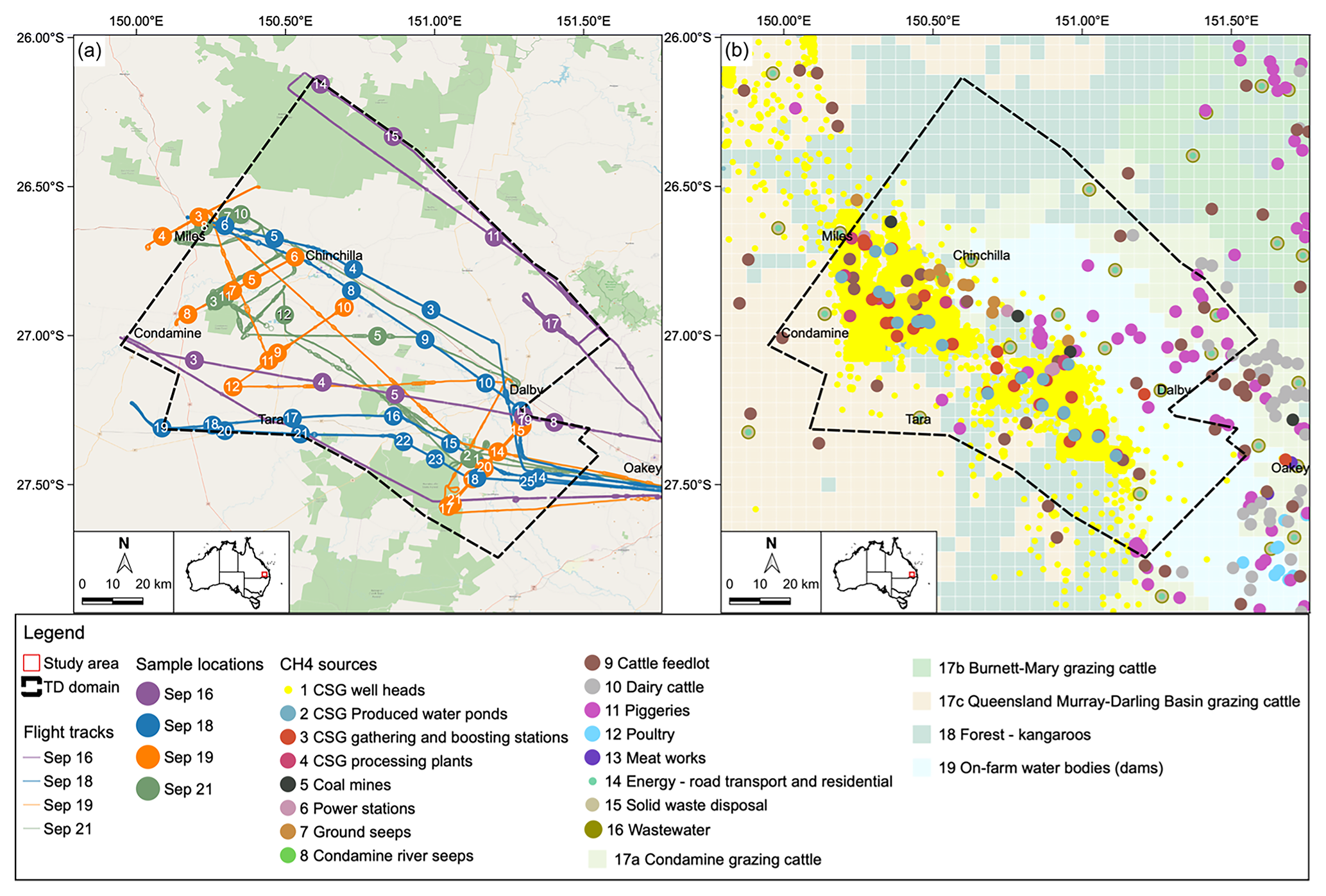
Figure 1Map of the study area with flight tracks and in-flight atmospheric air (IFAA) sample locations (a) (inset map shows the location in southeastern Queensland) and map of the CH4 sources in the area (b). (Inset map data: Australian Government (2020c), Administrative Boundaries © Geoscape Australia; base map and data from OpenStreetMap and OpenStreetMap Foundation). The black dashed polygon shows the extent of the TD domain, where the strong correlation between the UNSW BU inventory and the TD mass balance emission estimate was established in Neininger et al. (2021). The diffuse CH4 emissions were determined for each Australian Bureau of Statistics district (Condamine, Burnett Mary, and Queensland Murray–Darling Basin) and land use (mixed cropping and grazing, irrigated agriculture, and forest) using annual agricultural production data.
2.2 BU and TD CH4 emission estimates in the Surat Basin
The UNSW BU inventory closely followed the methods outlined in Australia's 2018 National Greenhouse Gas Inventory (Australian Government, 2020a). The UNSW inventory covers known sources such as those from the CSG industry and agriculture as well as sources discovered during the 2018 ground campaign in the study area (Lu et al., 2021). The inventory was collated using publicly available data. These data were supplemented with information from environmental impact approval reports, government and industry documents, close inspection of the satellite imagery in Google Earth, and airborne and ground survey observations (discussed in Lu et al., 2021, and Neininger et al., 2021). The locations of the sources contained in the UNSW inventory are shown in Fig. 1b.
In Fig. 2a all point sources (CSG facilities, feedlots, coal mines, etc.) are presented as an emission intensity map, and in Fig. 2b the distributed sources are shown. Distributed sources are multiple small sources spread evenly over a subregion. For example, we know the total number of cattle within a statistical district (Condamine, Burnett Mary, and Queensland Murray–Darling Basin) but not their locations, so the emissions are spread evenly using the population density. Comprehensive details about how the emissions from distributed sources were determined are discussed in Neininger et al. (2021, their Supplement, Sect. S). CSG sources are concentrated in a northwest to southeast zone, with agricultural sources on either side. The UNSW inventory estimate for the CH4 emissions in the southeast portion of the Surat Basin CSG fields for 2018 is 20 900 kg h−1 (183 Gg yr−1). In the UNSW inventory most of the emissions come from cattle, which contribute 50.3 % (29.9 % from grazing cattle, 19.1 % from feedlots, and 1.3 % from dairy cattle); all CSG sources contribute 30.5 %, piggeries 8.7 %, coal mines 7.6 %, and all other sources only 2.9 %. Within the airborne measurement TD domain, the UNSW inventory estimate for CH4 emissions is 11 500 kg h−1 (101 Gg yr−1), and the percentage contribution order within the TD domain is different: CSG 53.7 %, feedlots 19.0 %, grazing cattle 14.1 %, piggeries 7.3 %, coal 3.5 %, and all other sources 2.4 %. The heterogeneity of the point source emission rate is visually apparent in Fig. 2a. Within the UNSW inventory domain, 50 % of point sources have an emission rate of less than 4.5 kg h−1. These point sources account for 59 % of the UNSW inventory total. The top 10 % have an emission rate exceeding 113 kg h−1. The 42 sources in the top 10 % account for 37.7 % of the UNSW inventory total. The largest individual source is an open-pit coal mine (27.28∘ S, 151.71∘ E; red square, Fig. 2a), which emits 843 kg h−1 (4.1 % of the UNSW inventory total). The second largest source is a feedlot (27.42∘ S, 151.14∘ E; orange square, Fig. 2a), which emits 563 kg h−1 (2.7 % of the UNSW inventory total). The largest CSG source is a raw water pond (26.96∘ S, 150.49∘ E; light green square, Fig. 2a), which emits 221 kg h−1 (1.1 % of the UNSW inventory total).
The distributed sources of CH4 are dominated by grazing cattle (dark red in Fig. 2b, 6.54 kg h−1 per 25 km2), followed by the irrigation farming district (light blue, 0.64 kg h−1 per 25 km2), and then the forested areas with kangaroos (purple, 0.09 kg h−1 per 25 km2). There may also be some termite emissions from the forest and agricultural areas, but these have not been quantified. Grazing cattle account for 29.9 % of the UNSW inventory total CH4 emissions, and the position of this large source of CH4 emissions is one of the largest uncertainties in the calculations below. To maintain soil health and grass cover, the grazing cattle are rotated through various fields, and at times the cattle also graze along the roadside. The forested areas with large kangaroo populations were estimated to contribute only 0.2 % of all CH4 emissions. The irrigated agricultural district was estimated to have diffuse CH4 emission sources contributing only 0.7 % towards the UNSW inventory total.
Using airborne measurement techniques, Neininger et al. (2021) quantified the CH4 emissions in the southeastern portion of the Surat Basin CSG fields and surrounding agricultural districts. In the September 2018 campaign, there were 10 flights (∼45 h) using a research motor glider operated by Airborne Research Australia (ARA). Neininger et al. (2021) showed that there was strong correlation between the TD CH4 flux estimate and the UNSW inventory. Within the airborne survey domain, the TD estimate was 13 500 kg h−1 (118 Gg yr−1), which is 1940 kg h−1 (17 Gg yr−1) higher than the UNSW inventory.
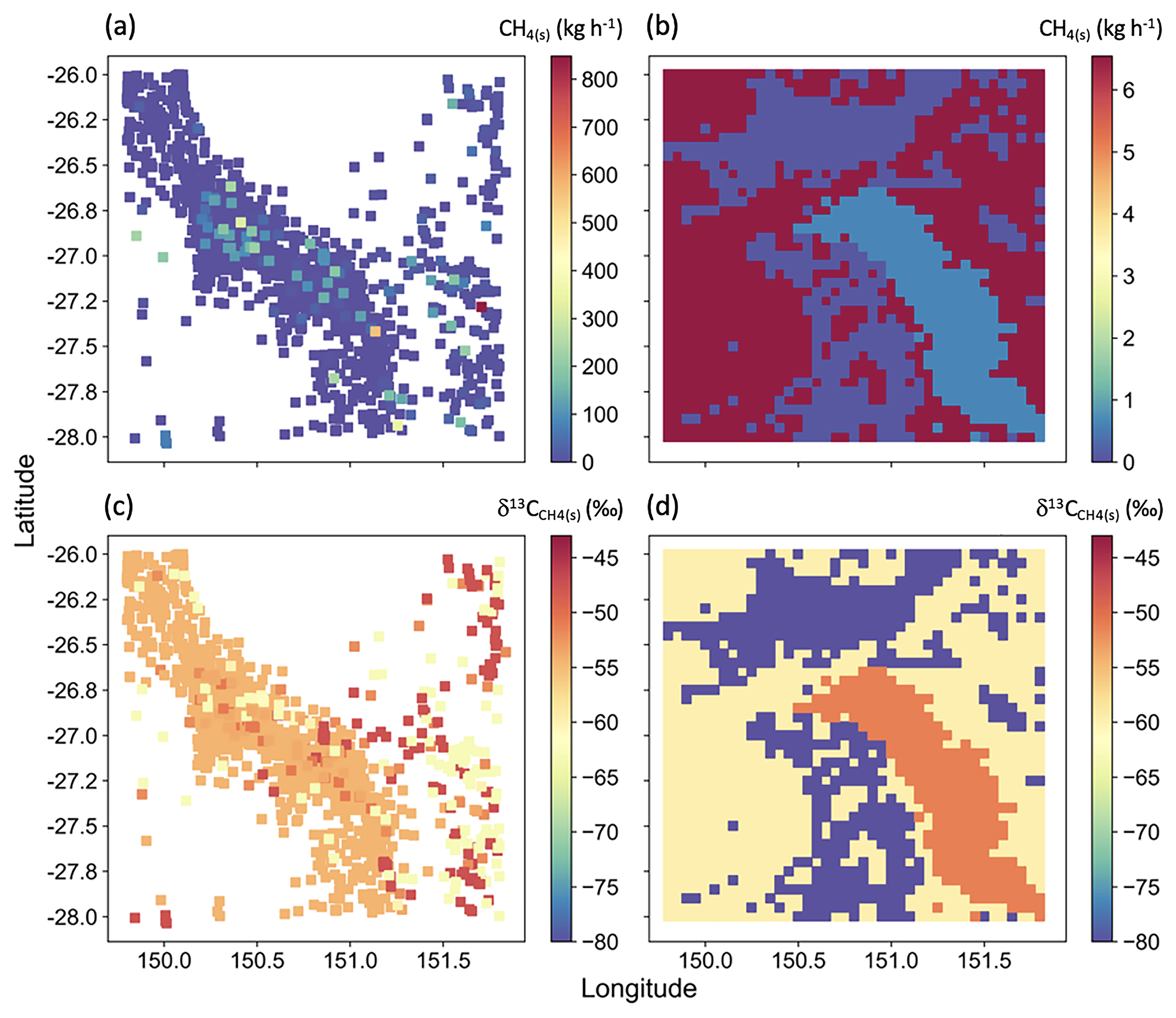
Figure 2Maps of the UNSW BU inventory (5×5 km for each grid cell) in the southeast portion of the Surat Basin CSG fields showing the estimated CH4(s) emissions for point (a) and distributed (b) sources and assigned δ13C for point (c) and distributed (d) sources.
2.3 δ13C signatures for each inventory category
The δ13C signatures of 16 primary sources in the Surat Basin were characterised in Lu et al. (2021) using air samples collected during ground-based surveys. These values are listed in Table A1 and were assigned to the different source categories in the inventory to create isotopic source signature maps. The spatial locations of the CH4 point sources and their corresponding δ13C values are shown in Fig. 2a and c. The distribution of the CH4 diffuse sources and corresponding δ13C values are shown in Fig. 2b and d. For many source types only one δ13C signature was determined in Lu et al. (2021). Gaining access to a wide range of farms and CSG facilities is difficult due to operational procedures and health and safety concerns. Therefore, an aim of this study was to examine if IFAA samples can be used to extend our knowledge of the CH4(s) signatures from various sources in the Surat Basin.
From the ground-based studies, the δ13C signatures from CSG processing and production facilities and CSG raw water ponds ranged from −56.7 ‰ to −45.6 ‰ (Bayesian 95 % credible interval (Crl); Lu et al., 2021). CSG is extracted from a range of depths in the Surat Basin gas fields. The shallowest coal measures tend to have a lighter isotopic signature and the deeper coal measures a heavier signature. This is due to the displacement of the original CH4 in coal seams nearest the ground surface with biologically derived CH4 (Iverach et al., 2015, 2017). The reported range for δ13C from gas from the Walloon Coal Measures is −64.1 ‰ to −44.5 ‰ (Baublys et al., 2015; Draper and Boreham, 2006; Hamilton et al., 2014, 2015; Iverach et al., 2015, 2017). The difference between the ground-based studies and well observations highlights the need to better characterise δ13C population statistics of CSG and other CH4 sources.
In addition to CSG sources of CH4 there are four major sources of CH4: feedlots, grazing cattle, piggeries, and coal mines (Neininger et al., 2021). For each of these sources only a single plume has been sampled to estimate δ13C; thus many more data sets need to be collected to robustly define the population statistics. A useful measure for the likely range of δ13C for each source category is summarised by the δ13C Bayesian CrIs, which for the limited sampling to date are as follows: feedlots, −65.2 ‰ to −60.3 ‰; grazing cattle, −61.7 ‰ to −57.5 ‰; piggeries −48.0 ‰ to −47.1 ‰; and coal mines, −61.1 ‰ to −58.9 ‰. Refer to Lu et al. (2021) for comprehensive details about how these δ13C signatures were determined and details about Bayesian regression.
For CH4 source categories listed in the BU inventories that were not sampled during the mobile survey, δ13C signatures were obtained from the literature. These include the δ13C signatures for kangaroos (−80 ‰, Godwin et al., 2014), on-farm waterbodies (dams) (−51.2 ‰, Day et al., 2016), and domestic wood heaters and native vegetation wildfires (−22.2 ‰, Ginty, 2016). There are also numerous termite mounds in the region, but there have been no studies on the rate of CH4 emissions from these mounds nor has δ13C been characterised for termites in the region. For worker termites collected from mounds near Darwin, Australia, Sugimoto et al. (1998) reported δ13C values ranging from −88.2 ‰ to −77.6 ‰. A major gas distribution line passes through the region; this transports conventional gas from the fields to the west of the study area to the LNG terminals on the coast and for the domestic market at Brisbane (Jemena, 2021). The δ13C population statistics for this gas are not known.
2.4 Research aircraft instrumentation and collection of the IFAA samples
Collecting IFAA samples in FlexFoil or similar bags is a comparatively fast and cost-effective method and has been used in numerous airborne and ground-based CH4 studies (Fisher et al., 2017; France et al., 2021; Lowry et al., 2020; Menoud et al., 2022b). During the campaign in September 2018, 92 IFAA samples were collected on board a Diamond Aircraft HK36TTC ECO-Dimona, equipped with underwing pods that housed the Los Gatos Research ultraportable greenhouse gas analyser and the modified LI-COR LI-7500 open path gas analyser for fast CO2 and H2O measurements and meteorological sensors for wind and thermodynamic parameters. Specifications of the airborne platform and instruments are described in Neininger et al. (2021). Sample bags were manually filled in the cockpit by connecting them to an air sampling tube, which had an inlet mounted far outside of the fuselage under the wing. Air was drawn into 3 L SKC FlexFoil PLUS (SKC Inc., USA) sample bags with polypropylene fittings. Ambient air was drawn from the intake with the assistance of a Viton membrane pump via polyurethane tubing. Before opening the valve of the sampling bags, the fitting was carefully flushed to avoid sampling cockpit air. The duration of bag filling was ∼ 1 min, which covers a track length of about 3 km at the flying speed of ∼ 170 km h−1. All IFAA samples presented in this study were collected within the convective boundary layer. During each flight, the top of the convective boundary layer was established several times by ascending and descending between the lower transects. During the surveying period, the convective boundary layer typically had an upper altitude limit ranging from 1700 to 2700 m a.g.l. (Neininger et al., 2021). Most of the airborne measurement surveying for the mass balance surveying and IFAA sampling was flown at altitudes of approximately 150 and 300 m a.g.l. (Fig. 3a). IFAA samples were collected on each transect, with up to 25 samples being collected in 1 d. When CH4 plumes were identified from the on-board real-time display, additional samples were collected. The IFAA sample locations for the 4 d analysed below are shown in Fig. 1a.
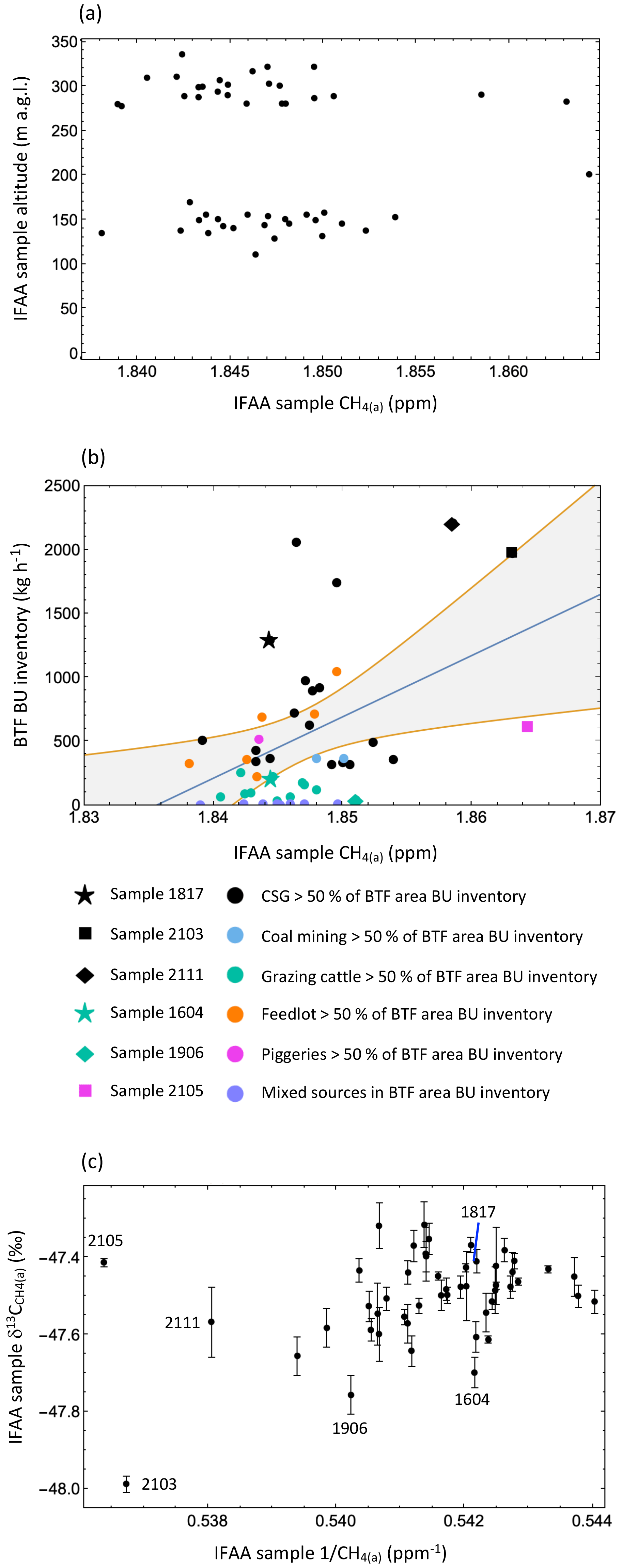
Figure 3IFAA sample observations between altitudes 100–350 m a.g.l. (a) IFAA sample altitude (m a.g.l.) versus IFAA sample CH4(a) (ppm). This plot highlights the sampling at altitudes of approximately 150 and 300 m. (b) Back-trajectory footprint bottom–up (BTF BU) inventory CH4 (kg h−1) versus IFAA sample CH4(a) (ppm). The linear regression fit highlights the moderate correlation (R2=0.59) between the two variables. The grey zone is the 95 % confidence level. (c) A Keeling plot: IFAA samples δ13C versus IFAA sample 1/CH4(a) (ppm). (The error bars are 1 standard deviation. For 1/CH4(a) the errors are too small to be observable; IFAA samples 1604, 1817, 1906, 2103, and 2105 are discussed in detail in the main text.)
When collecting IFAA samples there are many sampling and logistical challenges. We collected 3 L samples of air to enable both on-site testing and accurate laboratory measurements, and we used SKC FlexFoil PLUS bags to reduce the cost of the project. Also, because the air samples were collected manually and stored in the cockpit, the number of samples collected in each sampling run was limited to a maximum of ∼ 15. A purpose-built sampling system that rapidly fills 1 L canisters would potentially enable in-plume higher mole fraction IFAA samples to be collected. The smaller canisters would also allow for more samples to be collected on each flight. More in-plume samples with higher CH4 mole fraction values would reduce the uncertainty in the derived δ13C signatures. However, if the plume is heterogenous there is also a risk that rapidly filling the canisters will not sample the highest mole fraction portions of the plume.
2.5 Calculation of the 2 h back-trajectory footprint BU inventory emissions
For each IFAA sample the back-trajectory footprint (BTF) was calculated using the NOAA Air Resources Laboratory's (ARL) HYSPLIT model (Draxler et al., 1998) (Fig. A1 in Appendix A). HYSPLIT was used for this study because it is publicly available, enabling the methods presented here to be replicated by others. The HYSPLIT model is widely used for tracking air parcel trajectories as well as calculating transport, dispersion, and deposition of pollutants and hazardous materials (Stein et al., 2015). In this study, we determine the contributing CH4 sources (from the UNSW BU inventory in Neininger et al., 2021) of an IFAA sample within a BTF based on the 2 h HYSPLIT back trajectory starting at the IFAA sampling height and at the mid-point of the IFAA sampling interval. The HYSPLIT back-trajectory calculations were done using the global data assimilation system (GDAS) 0.5∘ meteorology option (GDAS 0.5∘, global September 2007–June 2019, using the normal trajectory, and for the vertical motion we selected to model the vertical velocity). The 2 h period was based on the forward and inverse plume modelling in Neininger et al. (2021), which established that most of the CH4 enhancement along a flight line could be attributed to a CH4 source located within 2 h, and within 0.025, 0.05, and 0.1∘ longitude/latitude on each side of the IFAA sample collection mid-point 1 and 2 h back-trajectory locations (refer to Fig. A1 for the HYSPLIT back trajectories and Fig. A2 for a representative BTF inventory polygon; also refer to Neininger et al. (2021), Supplement, Fig. SF26, for an example of the more detailed back-trajectory modelling, used to guide the HYSPLIT settings). Using the HYSPLIT BTF to determine contributing sources is an easy-to-replicate method. A more rigorous method would involve forward modelling the mixing of plumes for the prevailing meteorological conditions. Given that there are over 6000 point and distributed CH4 sources in the region, it is beyond the scope of this project to model the plume extending from each source and δ13C mixing. For the goal of identifying major upwind sources of CH4, the HYSPLIT BTF results compared favourably when checked against the higher-resolution local-scale modelling in Neininger et al. (2021). As the wind speeds changed throughout the sampling campaign this results in a different BTF for each sample. However, as will be shown below, for the purpose of identifying inventory knowledge gaps and mitigation opportunities, the variations in the BTF land surface area analysed are not critical for this study.
2.6 IFAA sample CH4(a) mole fraction and δ13C measurements
All CH4 mole fractions and δ13C values reported below were measured in the greenhouse gas laboratory at Royal Holloway, University of London (RHUL) (Fisher et al., 2006). For quality control, the IFAA samples were analysed on-site prior to shipping to the UK using a Picarro G2201-i cavity ring-down spectrometer (CRDS) (Picarro, Inc., USA). This was done to check for contamination during transportation to RHUL. If the UNSW and RHUL CH4 mole fraction values had a relative difference of greater than 1 %, the samples were removed and not analysed further. Forty-nine useable IFAA samples were collected. These samples had a median CH4 mole fraction difference of 0.4 % between the UNSW and RHUL measurements. The Picarro G2201-i used for this quality control step had been previously calibrated via an interlaboratory comparison between the Commonwealth Scientific and Industrial Research Organisation (CSIRO), UNSW, and RHUL. This calibration used Southern Ocean air from 2014 and 2016. Comprehensive details of the Picarro G2201-i performance are discussed in Lu et al. (2021). To control for any potential instrument drift, standardised Southern Ocean air was analysed at regular intervals, typically every 120 min, and if required, a drift correction was applied.
At RHUL, a Picarro G1301 CRDS (Picarro, Inc., USA) and a modified gas chromatography isotope ratio mass spectrometry (GC-IRMS) system (trace gas and isoprime mass spectrometer, Elementar UK Ltd., UK) (Fisher et al., 2006) were used for the measurement of CH4 mole fraction and δ13C, respectively. The Picarro G1301 CRDS has a reproducibility of ±0.0003 ppm. Air standards from the National Oceanic and Atmospheric Administration (NOAA) were used to calibrate the CRDS to the WMO X2004A scale (Dlugokencky et al., 2005; WMO, 2020). The CH4(a) mole fraction of each IFAA sample was determined by analysing the sample for 210 s on the Picarro G1301, and the average value of the last 90 s was recorded. All IFAA samples were measured in triplicate to obtain δ13C on the Vienna Pee Dee Belemnite (VPDB) scale using GC-IRMS. When the standard deviation of the first three analyses was greater than the target instrument precision of 0.05 ‰, a fourth analysis was performed. For more detailed information about the instrumentation and measurement procedure, see Fisher et al. (2006) and Lu et al. (2021).
2.7 Points of interest identification and application of multi-Keeling-model regression
Different CH4 formation processes result in each CH4 source having different δ13C population statistics for both the range and distribution shape (Whiticar, 1999; Sherwood et al., 2017, 2020; Menoud et al., 2022a). Thus, the isotopic composition of air samples can be used to identify inputs from similar sources, the extent of mixing of two or more sources, and samples that are offset to the isotopic composition expected from the BU inventory. IFAA samples of interest are those that have relatively high CH4(a) or different than expected δ13C (below called points of interest) because these samples may indicate over- or underestimation of CH4 emissions in the BU inventory. The points of interest can also indicate that a source of CH4 has been missed in the BU inventory. A point of interest may also indicate sampling or measurement errors, but this is unlikely for the samples analysed, due to the quality assurance measures at all stages of sampling and measurement.
Subsets of samples were collated based on altitude (Fig. 3a) and the dominant CH4 source in the BTF BU inventory (Tables A2, A3 and A4). Before sorting the data into subsets, points of interest were identified by visual inspection using two graphs: the BTF BU inventory vs. IFAA sample CH4 (Fig. 3b) and a Keeling plot (δ13C vs. 1/CH4(a)) (Fig. 3c). Although the points of interest were removed for the Keeling-model regression analysis, they are still analysed in the context of their position within the Keeling plot (Fig. 3c). After the points of interest were identified, the IFAA samples that had a single source that represented over 50 % of the 2 h back-trajectory inventory were combined into sets for the multi-Keeling-model regression with shared parameters analysis. Keeling analysis sets for the following categories were collated:
-
CSG > 50 % BTF BU inventory, 100–200 m a.g.l.
-
CSG > 50 % BTF BU inventory, 250–350 m a.g.l.
-
grazing cattle > 50 % BTF BU inventory, 100–200 m a.g.l.
-
grazing cattle > 50 % BTF BU inventory, 250–350 m a.g.l.
-
feedlots > 50 % BTF BU inventory, 100–350 m a.g.l.
The > 50 % threshold was set to achieve a balance between reducing the uncertainty in the regression and having a predominant CH4 source type in the upwind inventory. Ideally a higher threshold would be used, but this would require the collection of a greater number of IFAA samples than done in this study. The derived δ13C signatures for each category will be affected by the threshold, but the relative insights about a category being isotopically heavier or lighter will not.
For coal mines and piggeries there are only two BTF BU inventories with > 50 % emissions from these sources (Tables A3 and A4). As a result, these categories could not be analysed using the modelling methods below. There is only one category for feedlots because there are too few points for the Keeling analysis in the 100–200 and 250–350 m a.g.l. data sets.
For two-endmember mixing (a source of CH4 mixed in background air), the δ13C signature of the source mixing in background air is calculated using the Keeling-model method (Keeling, 1961; Pataki et al., 2003). The Keeling model is
where CH4(a) and δ13C are the IFAA sample values, CH4(b) and δ13C are the background-air values, and δ13C is the isotopic composition of the source.
In this study, for each source category 4 to 10 IFAA samples were collected where a single-source category contributed > 50 % of the BTF BU inventory emissions. For each category the samples were collected on different days and each day would have subtly different CH4(b) and δ13C. Regression of a single-source data set is poorly constrained, resulting in large uncertainties in the derived δ13C due to the low enhancement above background (less than 0.040 ppm) and the small number of samples in each category (Appendix B). To improve the confidence in the derived δ13C, δ13C, and CH4(b), the Keeling model (Eq. 1) was fitted simultaneously to all source category data sets using multi-Keeling-model regression with shared parameters (CH4(b) and δ13C), calculated using the MultiNonlinearModelFit function in Mathematica (Version 12.0) (Wolfram Research Inc., 2019). This algorithm globally optimises δ13C for each category and returns the shared values for CH4(b) and δ13C. Comprehensive details about the Mathematica MultiNonlinearModelFit function for fitting multiple data sets to multiple expressions that share parameters are available from the Wolfram function repository (Smit, 1986).
When the multi-Keeling-model regression with shared parameters is applied globally to all category data sets, the values for δ13C, δ13C, δ13C(Grazing-100to200), δ13C, and δ13C are unconstrained (allowed to vary during the regression). Background-air CH4(b) and δ13C are also unconstrained, and a single optimal set is determined. This assumes that CH4(b) and δ13C are similar on all days, which both the continuous ground surveying and airborne measurements results support (Lu et al., 2021; Neininger et al., 2021). This assumption is discussed further in Sect. 3.3.1. Because there are subtle changes in CH4(b) and δ13C throughout the campaign the multi-Keeling-model regression-determined values for CH4(b) and δ13C represent the background-air centroid for all days of measurements.
Miller and Tans (2003) discussed rearranging Eq. (1) for different data collection scenarios and regression aims. One algebraic expression rearrangement enables the source signature to be determined when CH4(b) and δ13C are unknown:
Like Eq. (1), when Eq. (2) is fitted to individual categories, it is poorly constrained for the dimensions of the data sets analysed.
A second algebraic expression rearrangement by Miller and Tans (2003) requires δ13C and CH4(b) to be specified:
For Eq. (3) CH4(b) and δ13C can be either constant or varying in time. A multi-Miller–Tans-model regression is equivalent to assuming constant CH4(b) and δ13C, and under this assumption fitting either Eq. (1) or (3) using multiple regression with shared CH4(b) and δ13C will result in the same values being determined for the shared CH4(b) and δ13C. Similarly, for each category almost identical values for CH4(b) and δ13C are determined within the precision of the simultaneous multiple regression calculations.
In Lu et al. (2021) Bayesian regression was used, and the credible interval (CrI) reported. The frequentist 95 % confidence interval (CI) is analogous to the Bayesian Crl (Lu et al., 2012; Albers et al., 2018). To allow direct comparison between this study and Lu et al. (2021), the 95 % confidence interval is reported below for δ13C.
A subset of visually identified points of interest (1604, 1906, and 2103), all with low δ13C values, is analysed using the results of the multi-Keeling-model regression. Using the values for CH4(b) and δ13C derived from the multi-Keeling-model regression, the Keeling model (Eq. 1) is fitted to this subset to determine its δ13C. For this subset a similar result could be obtained using Eq. (2).
3.1 IFAA sample locations and CH4 enhancement relationships
In Fig. 1 the location of the IFAA samples is shown. Most of the samples were collected near or above the CSG fields. As part of the surveying on both the 16 and 18 September 2018, IFAA samples were collected remote from CSG production above the agricultural districts. Figure 3a shows that the IFAA samples were collected at two focused-altitude intervals: between 100 and 200 m a.g.l., with most IFAA samples collected at approximately 150 m a.g.l., and between 250 and 350 m a.g.l., with most samples collected at approximately 300 m a.g.l.
A plot of the BTF BU inventory emissions (kg h−1) versus IFAA sample CH4(a) (ppm) shows that there is a moderate correlation (R2=0.59) (Fig. 3b). This moderate correlation is expected because the mixing of multiple CH4 sources under turbulent atmospheric conditions is not a linear process, the inventory is calculated using annual data, and the rate of emissions for many CH4 sources in the inventory will vary either throughout the seasons (agriculture) or daily (for example, CSG production or grazing cattle location). In Fig. 3c three samples have relatively high CH4(a) values (IFAA samples 2103, 2105, and 2111), and these points are discussed in detail below. IFAA sample 1817 is highlighted, as it is discussed in Sect. 3.4.
The IFAA samples are shown in a Keeling plot (Fig. 3c). In this graph three points with relatively low δ13C measurements are highlighted: 1604, 1906, and 2103. These three points were not included in the initial Keeling analysis but are analysed using insights from the multi-Keeling-model regression.
3.2 IFAA samples δ13C versus BTF BU inventory source category contribution
The 2 h back trajectories calculated using HYSPLIT for each day are shown in Fig. A1 and for each category set in Figs. A3, A4, and A5. The total emissions from each IFAA sample's HYSPLIT BTF were determined based on the UNSW BU inventory (Neininger et al., 2021, their Supplement) and listed in column 8, Table A2. The total CH4 emissions in each IFAA sample's BTF range from 2.7 to 2209.1 kg h−1 (each BTF BU inventory is a subset of the UNSW inventory). Five source categories account for most of the CH4 emissions in the Surat Basin: CSG, feedlots, grazing cattle, piggeries, and coal mine emissions (Neininger et al., 2021). The contribution of the individual source categories to the total emissions in the BTF were calculated as outlined in Neininger et al. (2021) and are expressed as percentages of the total emissions in Fig. 4.
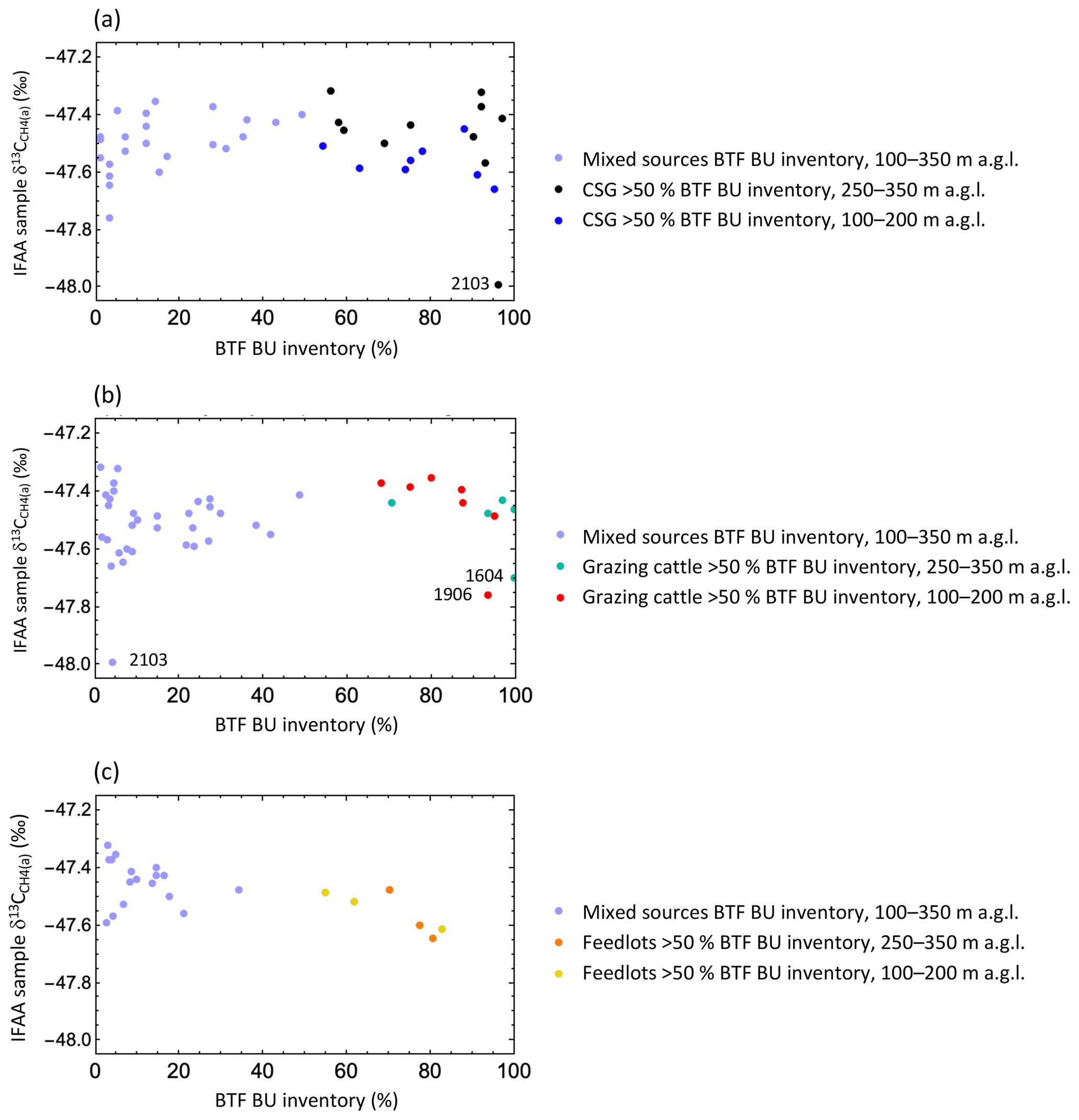
Figure 4IFAA sample δ13C (‰) versus percentage of BTF BU inventory emissions of the source categories indicated in the figure titles (%). (a) BTF BU inventories with CSG CH4 contributions; IFAA sample 2103 was excluded from the Keeling modelling set. (b) BTF BU inventories with grazing cattle CH4 contributions; IFAA samples 1604, 1906, and 2103 were excluded from the Keeling modelling sets. (c) BTF BU inventories with feedlot CH4 contributions. Category sets used in the Keeling plot modelling are each indicated by a separate colour, as shown in the colour keys. Samples below the 50 % BTF BU inventory threshold were excluded from the Keeling modelling.
There are three unknown parameters in the Keeling model (Eq. 1) (δ13C, CH4(b), and δ13C) and one independent variable (CH4(a) (x axis 1/CH4(a) in the Keeling plot)). To fit the Keeling model (Eq. 1) using the NonLinearModelFit and MultiNonlinearModelFit functions in Mathematica, a minimum of four IFAA samples is required (four CH4(a) and δ13C pairs).
For inclusion in the Keeling analysis input set for each CH4 source category, an individual source (CSG, grazing cattle, or feedlots) had to contribute > 50 % of the BTF CH4 emissions (Tables A3 and A4). The 50 % threshold was set to have enough points in each Keeling modelling set and still have one source potentially dominate the emissions. For each source category the set of samples that matched the threshold criteria is highlighted in colour in Fig. 4 and Tables A2, A3, and A4. IFAA samples excluded from the initial Keeling analysis are labelled in Fig. 4a and b. The HYSPLIT back trajectories for each IFAA sample are shown in Figs. A3, A4, and A5. These trajectories highlight that neither a single-point source nor a plume was sampled. Rather multiple plumes, where one source category dominated emissions, were analysed as a set (Fig. 4).
3.3 Multi-Keeling-model regression using shared parameters
In Fig. 5a the result of using multi-Keeling-model regression with shared background CH4(b) and δ13C is shown, and the regression statistics are summarised in Table A5. Because CH4(b) and δ13C are shared parameters, all Keeling lines converge to a common point for background air. The resulting values of this regression for the mole fraction and isotopic composition of the background are discussed below.
In Fig. 5b the result of using multi-Miller–Tans-model regression with shared background CH4(b) and δ13C is shown, and the regression statistics are summarised in Table A5. As expected, these are within measurement error identical to the Keeling-model results. For this reason, the results below are discussed with reference only to the Keeling-model algebraic expression representation of the two-endmember mixing model. For the reader interested in seeing the results of fitting the Keeling (Eq. 1) and Miller–Tans (Eq. 2) models to the individual categories, they are presented in Appendix B.
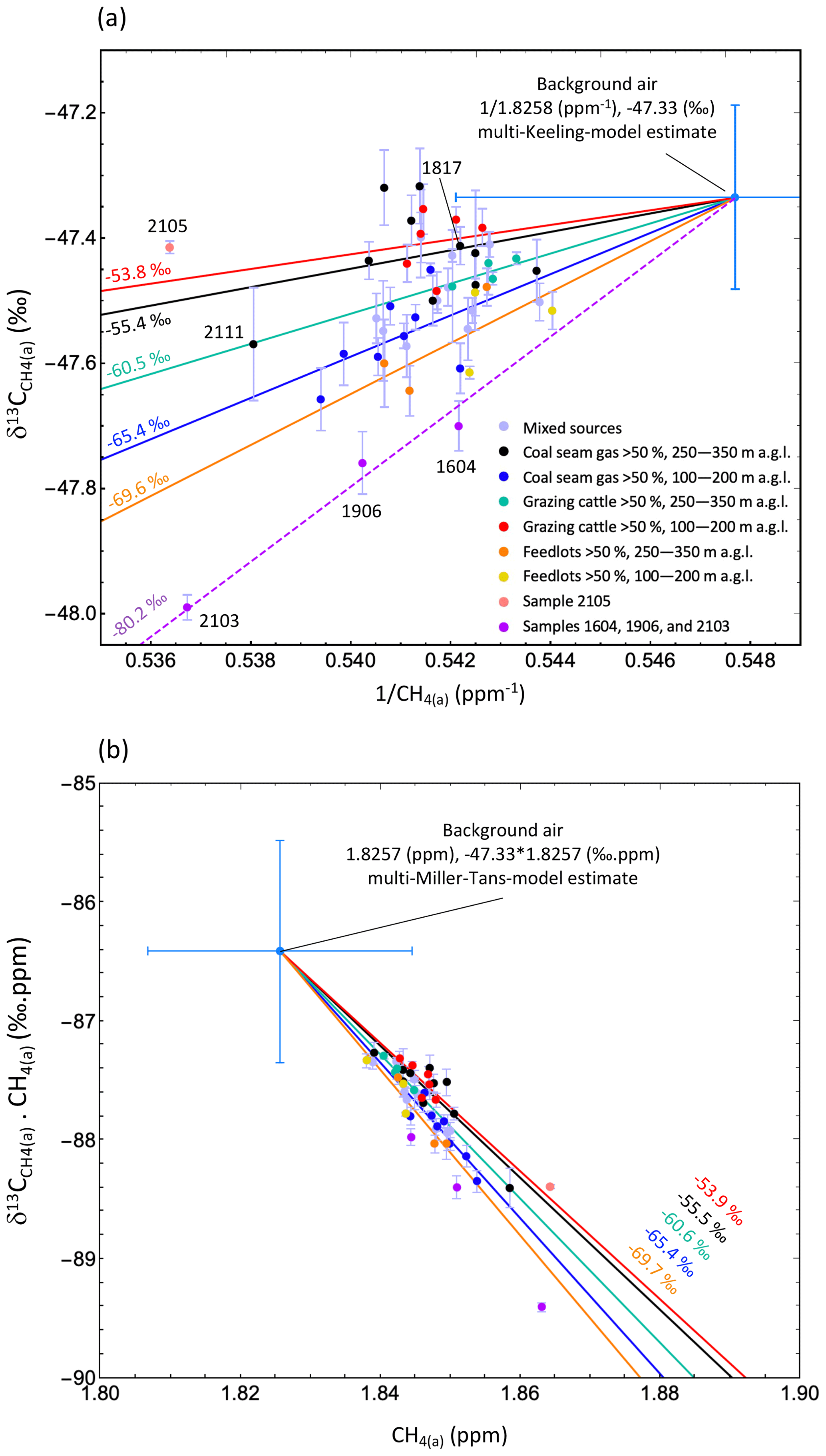
Figure 5Multiple regression with shared CH4(b) and δ13C for the Keeling model (a, solid lines, Eq. 1) and the Miller–Tans model (b, solid lines, Eq. 3) for the category subsets listed in the colour key. Refer to Table A5 for all regression results and their error statistics. The δ13C signature for each category is listed near the lines of best fit for each category. The dashed purple line in (a) shows a Keeling model (Eq. 1) fitted to IFAA samples 1604, 1906, and 2103 (for this regression CH4(b) and δ13C were fixed to match the results of the multi-Keeling-model regression with shared CH4(b) and δ13C). To highlight the subtle differences in the multiple regression best-fit parameters, the derived CH4(b) and δ13C values are given to an extra significant figure in (a) and (b) compared to the measurement precision. All error bars are 1 standard deviation.
3.3.1 Background air (CH4(b) and δ13C)
In a region with so many sources (Figs. 1 and 2), collecting IFAA samples to define both background CH4(b) and δ13C was not successful. Each day IFAA samples were collected remote from sources (Fig. 1a) with the aim of providing data to define background CH4(b) and δ13C. Subsequent analysis of all the IFAA samples indicated that none of the IFAA samples matched the low CH4 mole fractions recorded in Neininger et al. (2021). The background CH4 mole fraction recorded in continuous airborne surveys in Neininger et al. (2021) was stable between days and varied between 1.822 and 1.827 ppm. This range was established over 2 weeks with varying wind directions. For the period analysed in this study the wind directions were southwest averaging 8.6 m s−1, 16 September 2018; north averaging 4.1 m s−1, 18 September 2018; northwest averaging 6.8 m s−1, 19 September 2018; and southeast averaging 5.4 m s−1, 21 September 2018 (Fig. A1). How the background CH4 mole fraction was defined each day is discussed at length in the supporting information of Neininger et al. (2021).
There is no official atmospheric greenhouse gas monitoring station in the Surat Basin or anywhere in Queensland. The closest monitoring station is at Cape Grim, 1500 km south, which for September 2018 recorded averages of 1.8300 ppm and −47.3 ‰ (https://capegrim.csiro.au/, last access: 8 December 2022).
During the multi-Keeling-model regression calculation, the values for CH4(b) and δ13C were allowed to vary. The resulting values for background air are CH4(b)=1.826 ppm (CI 95 % ± 0.037 ppm) and δ13C ‰ (CI 95 % ± 0.3 ‰). This result falls within the CH4(b) range reported in Neininger et al. (2021) (between 1.822 and 1.827 ppm), and δ13C matches the Cape Grim value for the corresponding month (−47.3 ‰). The good match of the regression-derived CH4(b) and δ13C with the independent measurements of CH4(b) and δ13C demonstrates that multi-Keeling-model regression is a useful methodology for obtaining insights about the isotopic composition of the atmosphere.
3.3.2 CSG > 50 % BTF BU inventory, 250–350 m a.g.l.
IFAA samples included in this set were collected on all days (16, 18, 19, and 21 September 2018) and under different prevailing wind directions (Fig. A3a). These samples were collected either directly over or immediately adjacent to the CSG fields, and the resulting δ13C signature can be considered representative of blended CSG CH4 sources. The IFAA sample-derived δ13C signature for CSG > 50 % BTF inventory, 250–350 m a.g.l., was −55.4 ‰ (CI 95 % ± 13.7 ‰, black line Figs. 5a and 6a), which is within the range listed in Table A1 (CrI: −56.7 ‰to −45.6 ‰, grey band Fig. 6a) for CSG sources measured in Lu et al. (2021). The large uncertainties are due to the small CH4 enhancement, the small number of samples in each category data set, and the fact that in most cases there will be some small measure of input from multiple endmembers, although everything is modelled as if there is two-endmember mixing (one source and one background air). The overlap between the calculated and expected δ13C is shown graphically in Fig. 6a. Figure 4a shows that 5 of the 10 sample points had more than 90 % of the emissions in the BTF BU inventory derived from CSG sources, and in each case most of the CH4 emissions were from CSG compression stations. This result further validates both the methodology used in this study and the results in Lu et al. (2021).
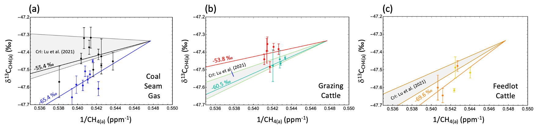
Figure 6Expected versus measured δ13C for each CH4 source category. The expected source category δ13C values from Lu et al. (2021), Table A1, are shown as thin continuous Keeling lines (without number values) for the upper and lower Bayesian credible interval for the category (where the credible interval is analogous to the 95 % confidence interval). The thick lines represent Keeling lines based on the IFAA samples (including derived source signatures). The IFAA sample point and measurement uncertainty are also shown for each category data set. The categories are (a) CSG > 50 % BTF inventory, 100–200 m a.g.l. (blue), and CSG > 50 % BTF inventory, 250–350 m a.g.l. (black); (b) grazing cattle > 50 % BTF inventory, 100–200 m a.g.l. (red), and grazing cattle > 50 % BTF inventory, 250–350 m a.g.l. (green); (c) feedlots > 50 % BTF inventory, 100–350 m a.g.l. (yellow points (100–200 m a.g.l.) and orange points (250–350 m a.g.l.)). All error bars are 1 standard deviation.
3.3.3 CSG > 50 % BTF BU inventory, 100–200 m a.g.l.
For the CSG > 50 % BTF BU inventory, 100–200 m a.g.l., set the δ13C signature was −65.4 ‰ (CI 95 % ± 13.3 ‰, blue line Figs. 5a, and 6a, also see Fig. A3b). This is considerably isotopically lighter than the higher-altitude CSG set discussed above and lower in value compared to all previous CSG measurements from Lu et al. (2021). The 100–200 m a.g.l. CSG δ13C signature is within the δ13C signature range reported in the literature for the Walloon Coal Measures (−64.1 ‰ to −44.5 ‰; Baublys et al., 2015; Draper and Boreham, 2006; Hamilton et al., 2014, 2015; Iverach et al., 2015, 2017) but is isotopically lighter than the range reported in Lu et al. (2021). In Fig. 6a all 100–200 m a.g.l. samples (blue points) are systematically isotopically lighter than the high-altitude, 250–350 m a.g.l. IFAA samples (black points). This offset is difficult to explain from the data collected.
With reference to the results in Tables A2, A3, and A4, the lower 100–200 m a.g.l. CSG set had no significant difference in the median CH4 compared to the higher 250–350 m a.g.l. set (1.849 to 1.847 ppm, respectively). However, there are two noticeable differences between the high- and low-altitude CSG sets: the median BTF BU inventory emission rate is 380 kg h−1 lower for the 100–200 m a.g.l. altitude set, and CSG sources for the 100–200 m a.g.l. set tally to a median emission rate that is 187 kg h−1 less than the 250–350 m a.g.l. CSG set. But these differences do not account for the lighter δ13C signature for the 100–200 m a.g.l. CSG set. There was also no significant difference between the low and high CSG BTF BU inventories with respect to either the grazing cattle or feedlot percentage inputs. Both CSG sets have samples collected on the 18, 19, and 21 September 2018; both sets cover a range of CSG areas (Fig. A3). In Fig. 6a all these lower-altitude samples where the upwind inventory is dominated by CSG sources are isotopically lighter than expected.
For three samples in the 100–200 m a.g.l. CSG set (1821, 1823 and 1911), greater than 88 % of the BU inventory emissions are due to CSG sources (Table A3); thus a δ13C value of −56.7 ‰ to −45.6 ‰ would be expected (Table A1). However, these samples are part of a category set that had a best-fit value of −65.4 ‰. Assuming that there are no major issues with the inventory, it would suggest that the ground-based study (Lu et al., 2021) did not capture the full δ13C population range for CSG sources. The low −65.4 ‰ value could also be explained by a higher proportional contribution from cattle emissions on the day of sampling or unaccounted emissions from termites. An additional possibility is that the air upwind of the 2 h limit is really a blend of background and other upwind sources and that the extent of enhancement of the air entering the 2 h limit was enough to invalidate the assumption of predominantly two-endmember mixing. Thus, an apparent source signature has been determined (Vardag et al., 2016). This possibility could be examined using a multisource transport model.
Ideally future chemical analysis of airborne collected air samples should include the measurement of δD to assist with constraining source attribution.
3.3.4 Grazing cattle > 50 % BTF BU inventory, 250–350 m a.g.l.
There were only four 250–350 m a.g.l. IFAA samples where grazing cattle contributed > 50 % of the BTF BU inventory emissions. These four points were clear of most other sources of emissions (Fig. A4a). The prevailing wind was from the southwest for sample 1603 and from the northeast for samples 1803, 1804, and 1805. Prior to sample collection the air had travelled over regions dominated by agriculture, mostly grazing cattle and mixed cropping. The multi-Keeling-model regression δ13C signature for the category grazing cattle > 50 % BTF BU inventory, 250–350 m a.g.l., was −60.5 ‰ (CI 95 % ± 15.6 ‰, Figs. 5a and 6b green line). This matches the grazing cattle result in Lu et al. (2021) (Fig. 6b grey band). This result indicates that in mixed cropping districts where grazing cattle are the dominant source of CH4 emissions, the expected and measured δ13C values align.
3.3.5 Grazing cattle > 50 % BTF BU inventory, 100–200 m a.g.l.
The multi-Keeling-model regression δ13C signature for the category grazing cattle > 50 % BTF BU inventory, 100–200 m a.g.l., was −53.8 ‰ (CI 95 % ± 17.4 ‰, Figs. 5a and 6b red line). This is too isotopically heavy for cattle and is closer to the expected value for CH4 emissions from CSG. Referring to Figs. 1a and A4b there are three possibilities that need further investigation.
The most likely explanation consistent with the source being within the 2 h BTF area is that there are numerous CSG production wells and associated gas pipelines and co-produced water pipelines (which have many high-point vents) immediately upwind of IFAA samples 1903, 1904, 1908, 1910, and 1912. Thus, there are numerous locations where venting could have been occurring on the day. In support of local CSG production causing the heavier than expected signature, IFAA sample 1808 plots on the grazing cattle line in Figs. 5a and 6b, and it has no CSG wells upwind (refer to the upper right inset Fig. A4b).
The second potential explanation is larger than expected urban CH4 emissions. IFAA sample 1910 is downwind of Chinchilla (population ∼ 6000), and 1912 is downwind of the towns of Condamine (population ∼ 400) and Drillham (population ∼ 130). In Table 2 there are four domestic sources of CH4 that could be contributing to the heavier than expected δ13C signature.
The third possible explanation is that CH4 emissions from the northwestern Surat Basin CSG facilities have been sampled in the north of the study area on 19 September 2018. Just beyond the 2 h back trajectories shown in Fig. A4b the air parcels would have travelled over the largest northwest Surat Basin gas fields near Woleebee Creek, which contains CSG plants, distribution hubs, and water treatment facilities. However, with reference to the modelling in Neininger et al. (2021) this is less likely compared to the first explanation that there are greater local CSG emissions than estimated in the inventory.
3.3.6 Feedlots > 50 % BTF inventory, 100–350 m a.g.l.
Due to too few points meeting the threshold requirement for the 100–200 and 250–350 m a.g.l. categories, the feedlot set was obtained by combining both altitude sets (Figs. 6c and A5). The derived multi-Keeling-model regression δ13C signature for the category feedlots > 50 % BTF inventory, 100–350 m a.g.l., was −69.6 ‰ (CI 95 % ± 22.6 ‰, Fig. 6c orange line), which is isotopically lighter than the −65.2 ‰ to −60.3 ‰ (CrI) listed for feedlots in Table A1 and shown in Fig. 6c (grey band) but still compatible within the derived 95 % confidence intervals. There are also too few values in the literature to fully characterise the population statistics for the δ13C signature of feedlot emissions in Australia, and this result may be simply better characterising the δ13C signature population range for feedlots. Another option to be explored as part of further ground studies is that there may be other isotopically lighter biological sources associated with the feedlots. For example, one of the feedlots sampled was Australia's largest feedlot (Grassdale), which has commercial-scale fertiliser production on site (https://www.grassdalefert.com.au/, last access: 8 December 2022), and this potential source of CH4 is not incorporated into any of the BU inventories for the region. This may be a biological source of CH4 with a lighter δ13C signature.
3.3.7 Analysis of the isotopically light IFAA samples
IFAA samples 1604, 1906, and 2103 are identified as being isotopically lighter compared to the other samples and were not used in any of the source category data sets. Using the multi-Keeling-model regression-derived background-air values (1.8258 ppm and −47.33 ‰), the Keeling model was fitted to 1604, 1906, and 2103 (Fig. 5a purple dashed Keeling line). The fitted model has a δ13C signature of −80.2 ‰ (CI 95 % ± 4.7 ‰). The only source listed in Table A1 that has this δ13C signature is kangaroos, but this would not be a significant CH4 source for these samples. There is another biological source of CH4 in the grazing cattle and mixed cropping districts that could be a contributor, upwind of IFAA samples 1604 and 1906. There are three sources of CH4 listed in Sherwood et al. (2017, 2020) and Menoud et al. (2022a) with δ13C signatures of −80 ‰: wetlands, waste, and termites. Of these three sources termites are the most likely, as termite mounds were observed during the field campaign in many of the forested and dryland farming regions. For IFAA sample 2103 both the brine water ponds and termites could be the missing biological source with a low δ13C signature. However, the relatively high CH4(a) measured for this sample (Figs. 3 and 5) suggests that the brine ponds, or another CSG source, are likely. Below, these isotopically light samples are discussed in detail with reference to satellite imagery.
3.4 Keeling plot points of interest
In Figs. 3 and 4 IFAA samples 1604, 1906, and 2103 are identified as points of interest because they are isotopically light. These points provide unique insights into overlooked sources of CH4 in the inventory and guide where further measurements are required.
IFAA sample 1604 was collected on the western margin of the CSG field (Fig. 7). It was initially anticipated to provide a background-air reference sample, but the δ13C of the air sample is −47.7 ‰, which is isotopically too light for fresh air in the Surat Basin. This sample sits on a Keeling regression line with a δ13C of −80.2 ‰. From our current knowledge of the region this cannot be assigned to a source. The back trajectory passes over regions of mixed cropping and cattle, and −80.2 ‰ is 20 ‰ lighter than expected for cattle in the region. There is a cluster of piggeries with a holding capacity of 10 000 just outside the near-distance BTF and another piggery cluster with a holding capacity of up to 25 000 pigs immediately upwind of the 2 h BTF. However, the one reported δ13C signature for piggeries in Lu et al. (2021) had a value of −47.6 ‰, so piggeries are highly unlikely to be the source. There are also a few CSG production wells in the area, but this source of CH4 is isotopically too heavy. A potential source that could explain the −80.2 ‰ signature in this farming district is termites.
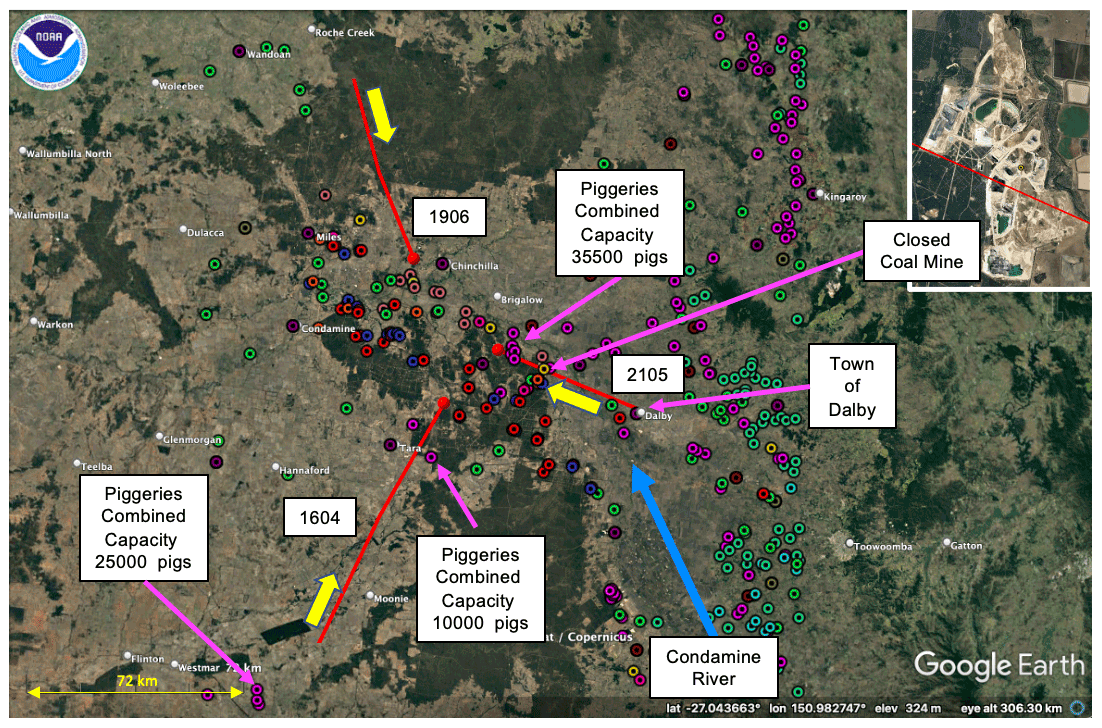
Figure 7Two-hour back-trajectory path lines (red) for IFAA samples 1604, 1906, and 2105. Refer to Fig. A1 for the point source colour key. Yellow arrows show the wind direction. The Condamine River flows from southeast to northwest (blue arrow) (image © Google Earth).
Upwind of IFAA sample 1906 no CH4 point source is recorded in the BU inventory (Fig. 7). There is a gravel quarry that has a small pond (200 m by 50 m) that could be a source of CH4 emissions with a biological signature. The only other known significant CH4 sources in this region are natural CH4 seeps and abandoned exploration well seeps (Lu et al., 2021). Many of these are coal exploration wells that intersect seams with a biological signature (Iverach et al., 2015; Lu et al., 2021), but these sources would be expected to have a δ13C signature of approximately −60 ‰, not the observed −80.2 ‰. Like sample 1604, the δ13C signature of −80.2 ‰ for sample 1906 could be explained by termites.
Sample 2105 (Figs. 3b and 7) is dominated by piggery emissions (56 %), which have a δ13C signature of −48.0 ‰ to −47.1 ‰ (CrI), with significant CSG emissions (36 %) and other minor sources (Tables A3 and A4). In Fig. 3b this point plots in a position suggesting that the inventory has underestimated emissions (Neininger et al., 2021). In Fig. 5a this point plots just above the CSG Keeling lines. A blend of piggery and CSG emissions accounts for both the relatively high CH4(a) and δ13C. A plausible explanation for this IFAA sample is that on the day of sampling CSG emissions were higher than indicated by the BTF BU inventory. Another possibility is that the emissions arise from a closed open-pit coal mine over which the back trajectory passes. Because this coal mine is closed it is not counted in the BU inventories. Large plumes intersected near this coal mine during the ground surveying presented in Lu et al. (2021), and emissions from this recently closed coal mine may have been captured in IFAA sample 2105. An additional possibility to be explored as part of new ground surveys is the emissions from natural seeps along the Condamine River.
The two IFAA samples with the highest CH4(a) mole fraction readings were downwind of the major CSG facilities (samples 2111 and 2103, Figs. 3, 4, and 8). Sample 2103 is of particular interest because it has the lowest δ13C of any sample collected, and it plots on the −80.2 ‰ Keeling line in Fig. 5a. The wind was moving from southeast to northwest when samples 2103 and 2111 were collected about 20 km west–northwest of the Kenya water management ponds (Fig. 8). The back-trajectory centre line for sample 2111 passes directly over the Berwyndale South/Windbri central processing plant and Talinga plant (Fig. 8b) and immediately to the north of the Kenya water management ponds (Fig. 8c). Sample 2111 is a blended input from all these facilities. CSG sources contributed 93 % towards the CH4 emissions in the BTF BU inventory: CSG wells, 245 kg h−1; CSG raw water ponds, 787 kg h−1; CSG compressor stations, 811 kg h−1; and CSG plants, 210 kg h−1 (Table A3). Feedlot cattle contributed 4 % (88 kg h−1) and grazing cattle 3 % (64 kg h−1) (Table A4).
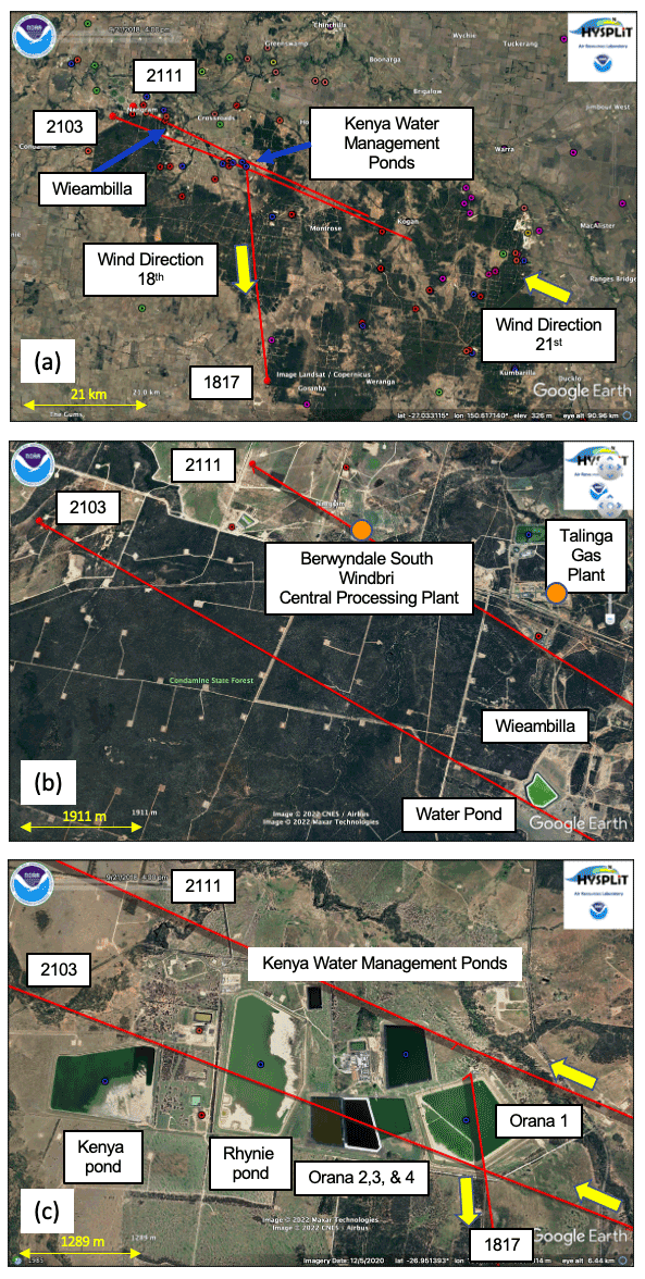
Figure 8(a) Two-hour back-trajectory path lines for IFAA samples 1817, 2103, and 2111. (b) Back-trajectory paths for 2103 and 2111 relative to the Berwyndale South/Windbri central processing plant and the Talinga processing plant. (c) Kenya water management ponds relative to 1817, 2103, and 2111 back-trajectory centre lines. The yellow arrows show the wind direction for each trajectory. Refer to Fig. A1 for the point source colour key (image © Google Earth).
The back-trajectory centre line for 2103 passes over two sets of ponds: ponds near Wieambilla in the proximal BTF and further east at the Kenya water treatment complex (Fig. 8a and c). Kenya pond holds treated water suitable for adding to the Condamine River (Fig. 7). Orana 4 holds brine produced from the filtering of the raw water before being sent to the brine concentrator. Orana 2 and 3 hold water output from the brine concentrator (QGC, 2013). No plumes were sampled near this complex in Lu et al. (2021), so the δ13C of any emissions from these ponds is not known. CSG sources contributed 96 % towards the emissions in the BTF BU inventory for sample 2103: CSG wells, 251 kg h−1; CSG raw water ponds, 586 kg h−1; CSG compressor stations, 714 kg h−1; and CSG plants, 338 kg h−1 (Table A3).
Sample 1817 (Figs. 3c, 5a, and 8) also has a back-trajectory line that passes over the Kenya water management ponds. It was collected 35 km south of the ponds and other major CSG facilities, which accounts for its lower CH4 mole fraction. The back-trajectory centre line for 1817 passes over the easternmost Kenya water management pond, Orana 1, which is a raw water pond. CH4 emitted from this pond is likely to have a similar composition to the produced gas. CSG sources contributed 97 % of the CH4 emissions in the BTF: CSG wells, 136 kg h−1; CSG raw water ponds, 582 kg h−1; CSG compressor stations, 459 kg h−1; and CSG plants, 78 kg h−1 (Table A3). For sample 1817 there was also a minor input from grazing cattle (2.5 %; 32.7 kg h−1; Table A4). This sample does not plot as an outlier (Figs. 3c and 5a).
Samples 1817 and 2111 plot in the Keeling plot (Fig. 5a) in positions consistent with our knowledge of the δ13C signatures of sources in the BTF BU inventory. To explain the position of sample 2103 in Fig. 5a a source of CH4 with a δ13C signature of approximately −80 ‰ is required. The size and position of the Kenya water management treatment complexes associated with the water treatment, the presence of brine ponds, and other waste together make this facility a potential location for the missing source of CH4 with an δ13C signature of approximately −80 ‰. The back trajectory also passes over forested areas where there are termites. Further fieldwork is required to answer why sample 2103 indicates a missing biological source of CH4 in the inventories.
An objective of this study was to use IFAA samples to investigate whether we could characterise the δ13C source signature of emissions from facilities that could not be sampled during the ground campaign (Lu et al., 2021), especially the CSG regions that are remote from public roads. To achieve this objective, we had to produce a BU inventory of both point and diffuse CH4 sources for the region. This inventory enabled us to sort the IFAA samples into sets based on the predominant 2 h upwind inventory source of CH4 (e.g. one sample per feedlot, for multiple feedlots). We were then able to determine the δ13C signature for a single-source category. The method worked with mixed results.
A concern after the measurements of the IFAA samples in the laboratory was that the lack of CH4(a) enhancement above CH4(b) (less than 0.04 ppm) would not allow for the interpretation of these data using the Keeling plot method. Establishing CH4(b) and δ13C, as traditionally done from the collated data sets, was not possible by fitting the Keeling model (Eq. 1) or the Miller–Tans model (Eq. 2) to individual data sets (this is demonstrated in Appendix B). We overcame this challenge with careful sample quality control and by using multi-Keeling-model regression with shared CH4(b) and δ13C. An interpretation in alignment with other ground and continuous airborne observations was possible only after applying this regression algorithm. Importantly, despite the low CH4(a) enhancement of less than 0.04 ppm, the derived values for background-air CH4(b)=1.826 ppm (CI 95 % ± 0.037 ppm) and δ13C ‰ (CI 95 % ± 0.3 ‰) match independent observations. Being able to assign a well-constrained value to CH4(b) and δ13C was central to the interpretation of all IFAA samples.
The derived δ13C values for the 250–350 m a.g.l. IFAA sample sets (Figs. 5a, 6a and b; Table A5) where the inventory was dominated by CSG facilities or grazing cattle were close to those determined from the ground-based analysis of plumes (Lu et al., 2021). It can be concluded that the upwind inventory for these samples was reasonably well characterised.
For IFAA samples collected downwind of the feedlots the derived multi-Keeling-model regression δ13C signature was isotopically lighter than expected by approximately 5 ‰. However, this category was poorly constrained and had a large 95 % confidence interval ranging from −92.2 ‰ to −47.0 ‰. A better data set is required to characterise the population statistics for feedlot CH4 emissions, especially since there are no uniform procedures for feedlot design and waste management.
The results for the 100–200 m a.g.l. altitude IFAA samples where the inventory was dominated by CSG facilities or grazing cattle did not match expectations and were isotopically lighter than expected (Figs. 5a, 6a and b; Table A5). There are many possible explanations that cannot be resolved using currently available data. The mismatch could be due to there being more than one dominant source category in the upwind region (with potential inputs from beyond the 2 h back trajectory), incomplete mixing of all sources, sources missing from the BU inventory, the applied emission factors used for source apportionment not being precise for the individual source, or the δ13C signatures from the few plumes sampled as part of the ground-based studies not being representative of the complete population statistics.
To constrain the interpretation, for each CH4 source the population distribution for both δ13C and δD needs to be better characterised. These data would enable the statistical modelling of inventories for better comparison with IFAA sample CH4(a) and δ13C data and be useful for atmospheric transport isotope mixing model studies, which have the potential to yield more insights about inventory knowledge gaps compared to the pragmatic methods used in this study. Due to the low enhancement in the mole fraction and the small number of samples collected with predominantly one inventory source category upwind, the derived δ13C signatures have large uncertainties. For the methods presented in this study to work more effectively, more samples are needed downwind of each source category, and the sampling containers should be filled as rapidly as possible.
A primary aim of the study was to see if the IFAA samples would be useful for identifying overlooked sources of CH4, and this was achieved. In Fig. 3c three points of interest were identified for their relatively low δ13C values: IFAA samples 1604, 1906, and 2103. Although this is a small subset, the insights obtained are important. The application of multi-Keeling-model regression with shared CH4(b) and δ13C constrained the δ13C signature for these samples to be approximately −80 ‰. For all three samples, termite emissions may have been sampled. For sample 2103, the upwind CSG brine ponds, or another CSG source close to these ponds, also need to be investigated as a potential source of CH4 that has not been incorporated into the BU inventories. The relatively high enhancement of atmospheric CH4 downwind of the CSG water management ponds indicates a potentially large CH4 source, which could be quantified in the future using a different sampling design (e.g. mass balance flight pattern or ground-based plume studies). CSG water management ponds may also represent a mitigation opportunity. Improved separation of the methane from the water at the production well head or before placing the water into the ponds would increase the resource produced and minimise fugitive CH4 emission.
The measurement of δ13C in this study has identified that termites are potentially contributing significant quantities of CH4 to the regional CH4 budget. Quantifying termite CH4 emissions from both natural and agricultural landscapes may help with closing the gap between the top–down and bottom–up CH4 emission estimates reported in Neininger et al. (2021). More generally, atmospheric measurements of greenhouse gas emissions using satellite-, aircraft-, and drone-based analysers are increasingly being used for inventory verification. The results presented in this study and in Basu et al. (2022) demonstrate that isotope studies are required to constrain source attribution. To further enhance our capacity to interpret atmospheric CH4 measurements, ideally both δ13C and δD should be measured (Lu et al., 2021).
The application of the multi-Keeling-model regression with shared CH4(b) and δ13C enables the following: the characterisation of the δ13C signatures for sources not accessible during ground campaigns assuming accurate source attribution in the inventory; the identification of coal seam gas subregions where there is poor agreement between the IFAA sample δ13C measurement and the δ13C value expected from the BU inventory; the identification of subregions where there must be a strong source of CH4 with a δ13C signature of approximately −80 ‰ not recorded in the BU inventories; and the identification of mitigation opportunities. The isotopic analysis methods presented in this study could be applied in any setting where there are many co-located sources of CH4 and be used to identify CH4 source knowledge gaps in national inventories.
A1 Abbreviations
| BTF | Back-trajectory footprint |
| BU | Bottom–up |
| CI | Confidence interval |
| Crl | Credible interval |
| CSG | Coal seam gas |
| CSIRO | Commonwealth Scientific and Industrial Research Organisation |
| CRDS | Cavity ring-down spectrometer |
| GC-IRMS | Gas chromatography isotope ratio mass spectrometry |
| HYSPLIT | Hybrid Single-Particle Lagrangian Integrated Trajectory |
| IFAA | In-flight atmospheric air |
| m a.g.l. | metres above ground level |
| NOAA | National Oceanic and Atmospheric Administration |
| RHUL | Royal Holloway, University of London |
| TD | Top–down |
| UNFCCC | United Nations Framework Convention on Climate Change |
| UNSW | University of New South Wales |
| VPDB | Vienna Pee Dee Belemnite |
A2 Tables
Table A1Surat Basin ground-based campaign (Lu et al., 2021) and literature δ13C values for each source category within the study area.
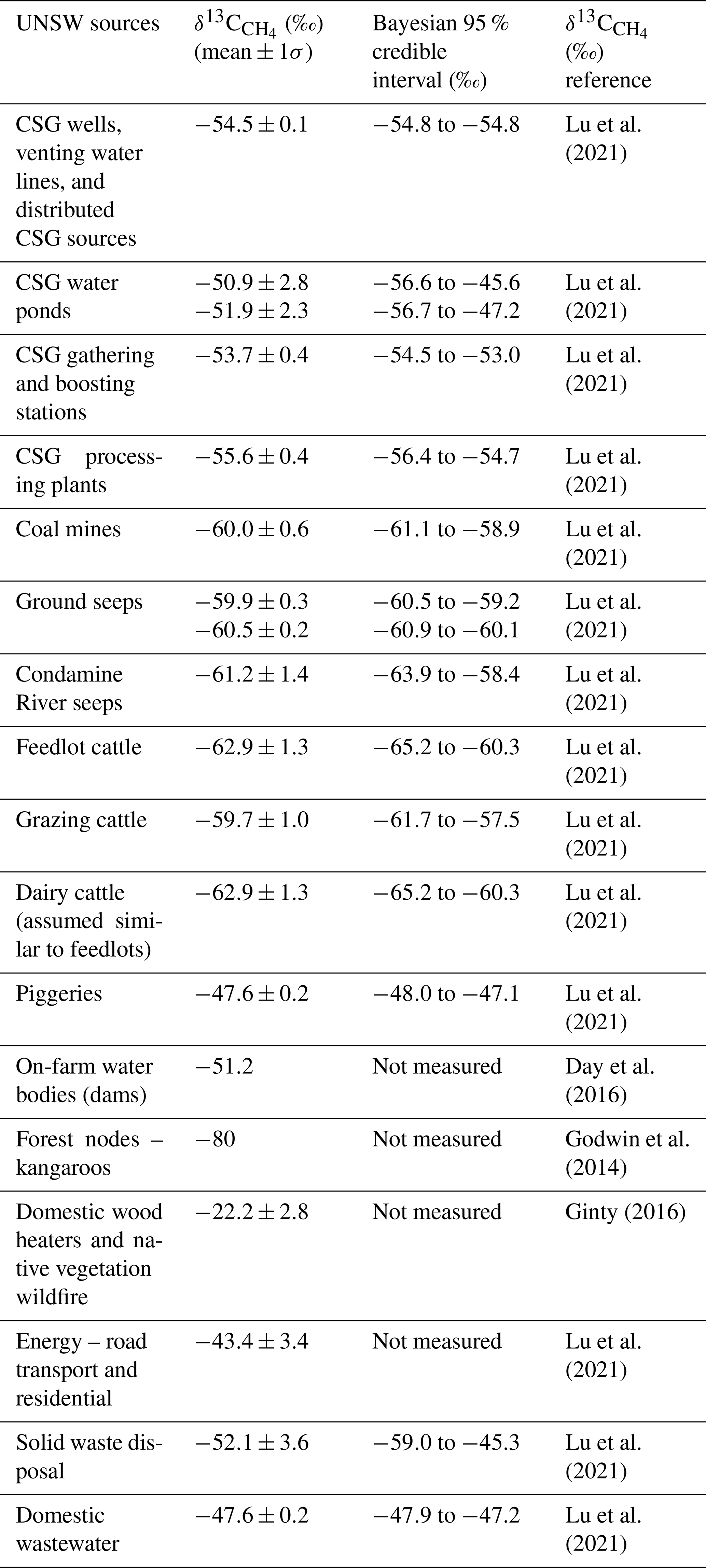
Table A2In-flight atmospheric air sample location details and UNSW bottom–up inventory CH4 emissions estimates within the 2 h back-trajectory footprint.
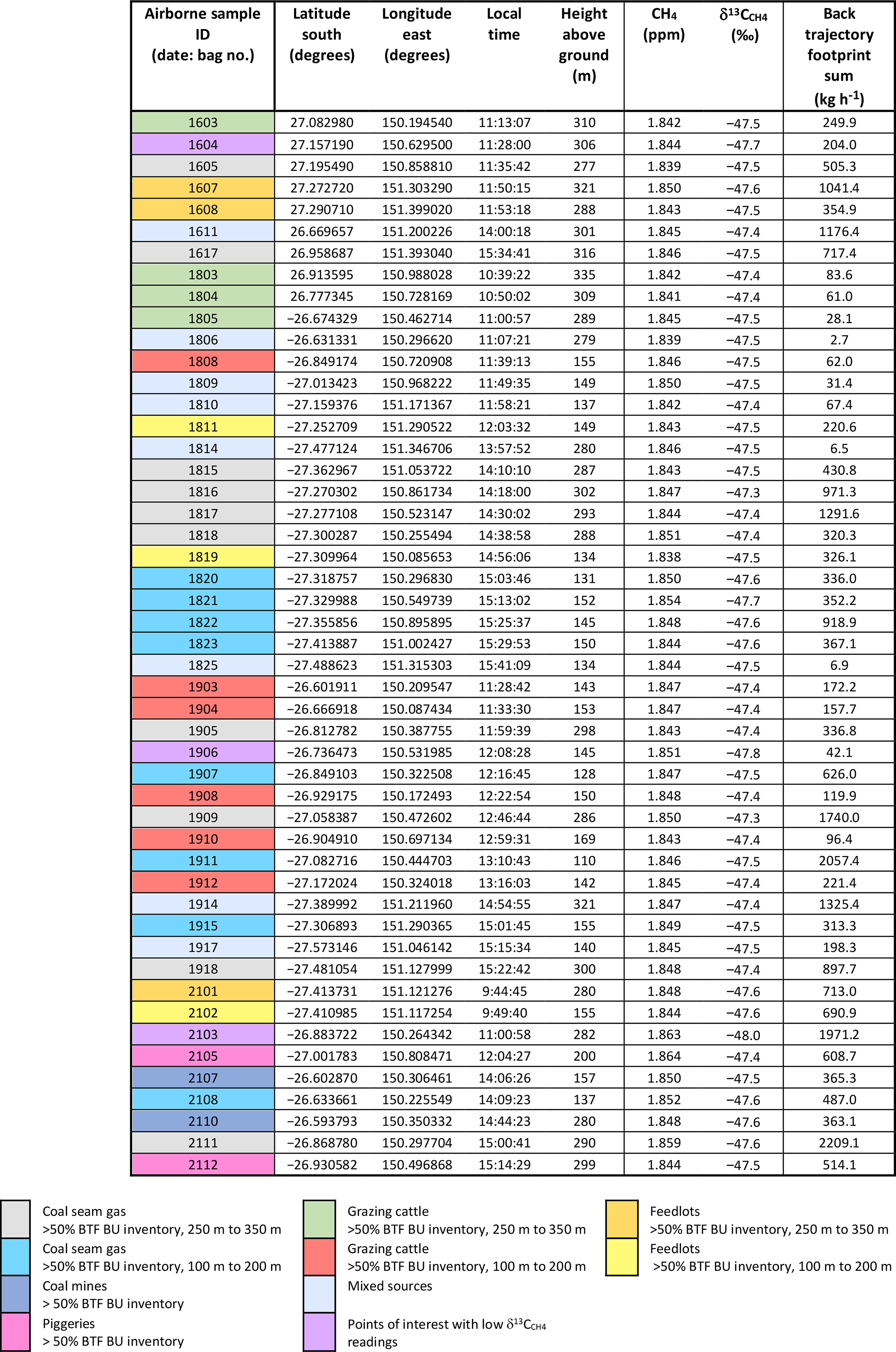
Table A3In-flight atmospheric air sample location details and UNSW bottom–up inventory CH4 emissions estimates for fossil fuel and minor mixed sources within the 2 h back-trajectory footprint.

Table A4In-flight atmospheric air sample location details and UNSW bottom–up inventory CH4 emissions estimates for major agricultural sources within the 2 h back-trajectory footprint (Australian Bureau of Statistics districts: Condamine Natural Resource Management (NRM) area and Queensland Murray–Darling Basin (MDB) Natural Resource Management (NRM) area).
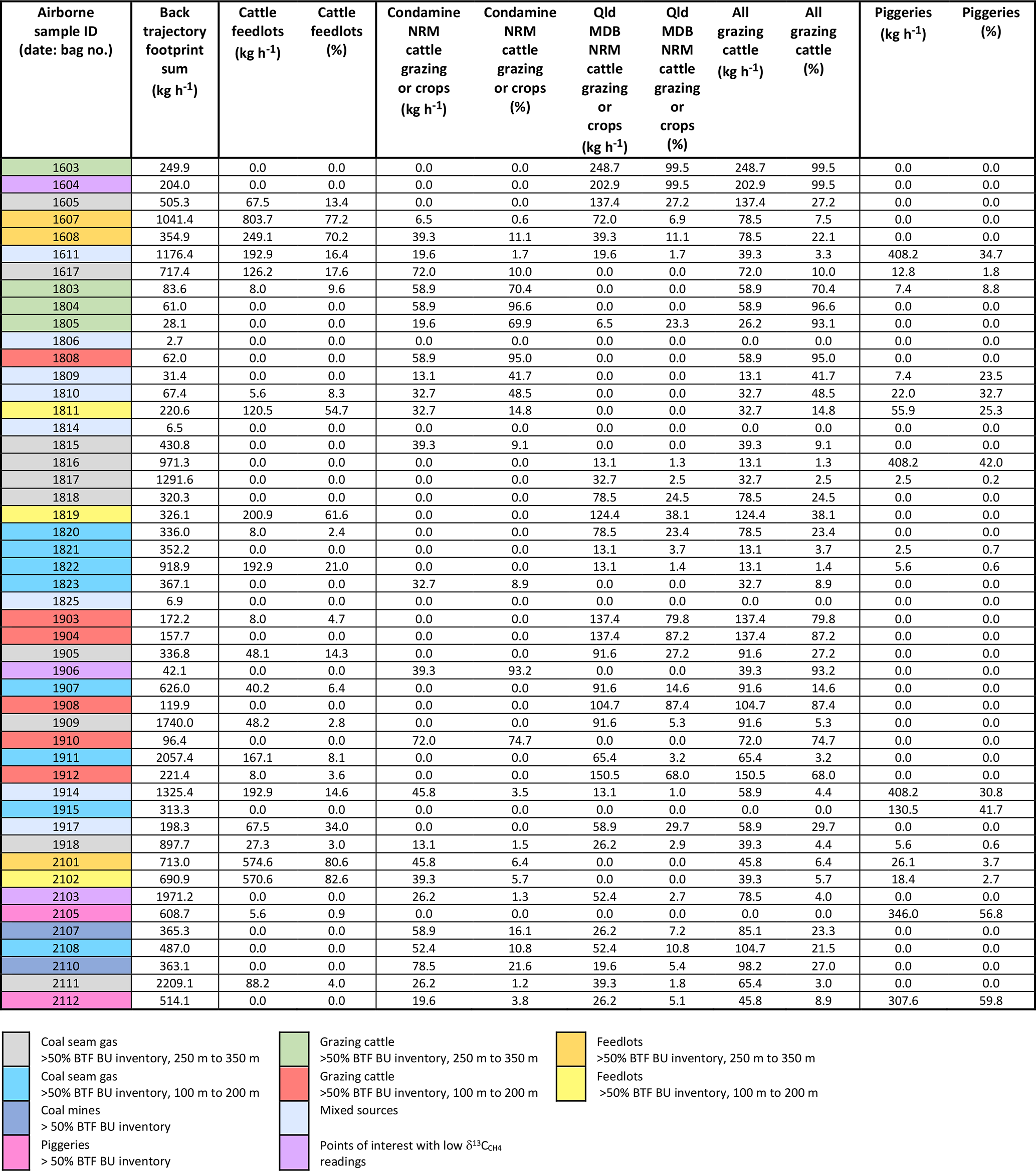
Table A5Calculated δ13C values using multi-Keeling-model regression with shared CH4(b) and δ13C and using multi-Miller–Tans-model regression with shared CH4(b) and δ13C.

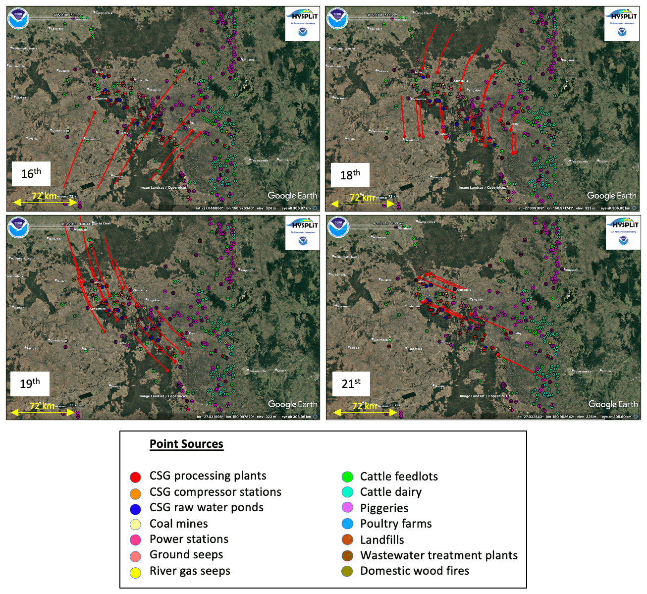
Figure A1Two-hour HYSPLIT back-trajectory path lines (red) for each day of IFAA sampling. The back trajectory starts at the mid-point of the air sample collection interval (circled end of the red line) (image © Google Earth).
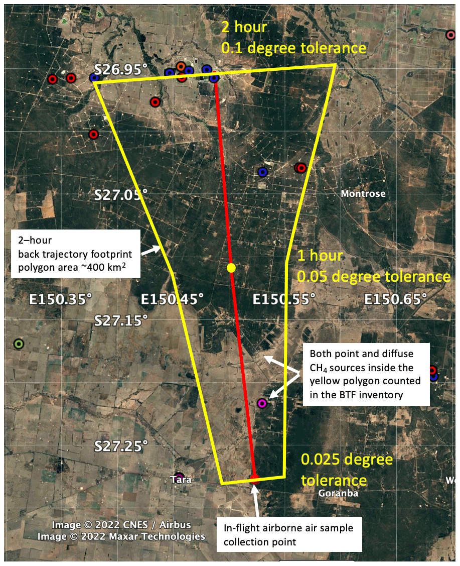
Figure A2A representative BTF inventory polygon for IFAA sample 1817. The red line shows the 2 h back trajectory determined using HYSPLIT. Refer to Fig. A1 for the point source colour key (image © Google Earth).
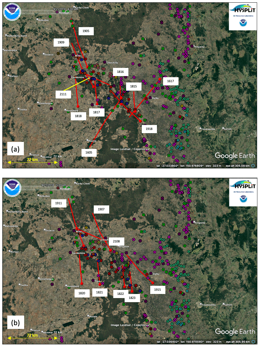
Figure A3Two-hour HYSPLIT back-trajectory path lines (red) for the points used in the coal seam gas Keeling-model regression analysis. (a) HYSPLIT back trajectories CSG > 50 % BU inventory, altitude 250–350 m a.g.l. (b) HYSPLIT back trajectories CSG > 50 % BU inventory, altitude 100–200 m a.g.l. Refer to Fig. A1 for the point source colour key (image © Google Earth).
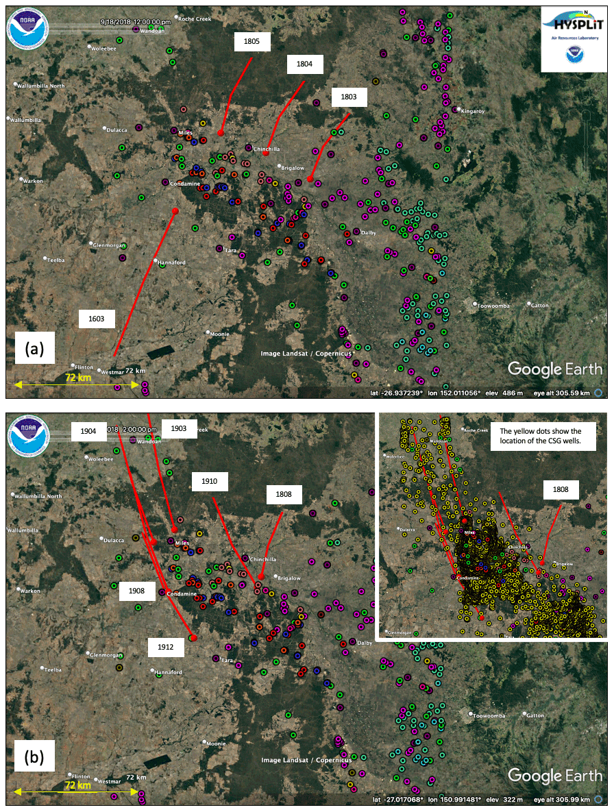
Figure A4Two-hour HYSPLIT back-trajectory path lines (red) for the points used in the grazing cattle Keeling-model regression analysis. (a) HYSPLIT back trajectories grazing cattle > 50 % BU inventory, altitude 250–350 m a.g.l. (b) HYSPLIT back trajectories grazing cattle > 50 % BU inventory, altitude 100–200 m a.g.l. Refer to Fig. A1 for the point source colour key (image © Google Earth).
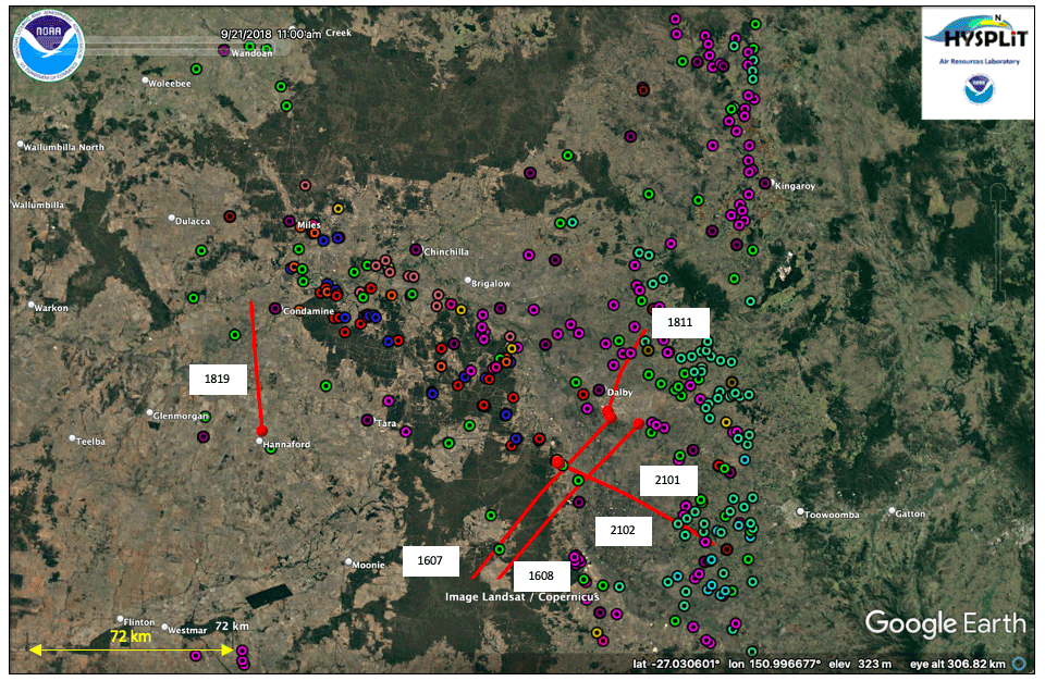
Figure A5Two-hour HYSPLIT back-trajectory path lines (red) for the points used in the feedlot Keeling-model regression analysis. Each green dot indicates the position of a feedlot (image © Google Earth).
A commonly used method to determine δ13C is to fit the Keeling model (Eq. 1) or Miller–Tans model (Eq. 2) to a set of air samples collected within a single plume. For the IFAA samples collected as part of this study, the combination of the low level of CH4 enhancement (<0.040 ppm) and the small number of samples in each category (<10 IFAA samples) results in poorly constrained regressions with large uncertainties (Table B1).
The single category Keeling-model (Eq. 1) results are presented in Fig. B1a to highlight the issue of fitting the Keeling model to small data sets with low CH4 enhancement above background CH4(b). The Keeling regression lines in Fig. B1a do not converge to a common point for CH4(b) and δ13C as would be expected given the stability of CH4(b) established during the continuous measurement airborne campaign (Neininger et al., 2021). Many of the regression lines converge far to the right of the CH4(b) and δ13C values determined from the simultaneous multiple regression. In addition, the uncertainty bars for the source signatures derived from the unconstrained fits are so large that no meaningful source attribution is possible (Table B1). The resulting δ13C signatures of the individual regressions for each category are as follows:
-
CSG > 50 % BTF BU inventory, 100–200 m a.g.l., −66.8 ‰ (CI 95 % ± 38.2 ‰);
-
CSG > 50 % BTF BU inventory, 250–350 m a.g.l., −54.6 ‰ (CI 95 % ± 23.9 ‰);
-
grazing cattle > 50 % BTF BU inventory, 100–200 m a.g.l., −60.7 ‰ (CI 95 % ± 60.7 ‰);
-
grazing cattle > 50 % BTF BU inventory, 250–350 m a.g.l., −65.3 ‰ (CI 95 % ± 146.1 ‰);
-
and feedlots > 50 % BTF BU inventory, 100–350 m a.g.l., −68.9 ‰ (CI 95 % ± 44.9 ‰).
When CH4(b) and δ13C are unknown, it is common to use the Miller–Tans model (Eq. 2) to determine δ13C. The results of fitting this model separately to the five category data sets are presented in Fig. B1b. Like the Keeling model, the regression lines of best fit do not converge to a common point for CH4(b) and δ13C. The 95 % confidence intervals are also large (Table B1). The resulting δ13C signatures of the individual regressions for each category are as follows:
-
CSG > 50 % BTF BU inventory, 100–200 m a.g.l., −66.9 ‰ (CI 95 % ± 38.1 ‰);
-
CSG > 50 % BTF BU inventory, 250–350 m a.g.l., −54.7 ‰ (CI 95 % ± 23.8 ‰);
-
grazing cattle > 50 % BTF BU inventory, 100–200 m a.g.l., −60.6 ‰ (CI 95 % ± 60.7 ‰);
-
grazing cattle > 50% BTF BU inventory, 250–350 m a.g.l., −65.3 ‰ (CI 95 % ± 146.1 ‰);
-
and feedlots > 50 % BTF BU inventory, 100–350 m a.g.l., −69.0 ‰ (CI 95 % ± 44.9 ‰).
These poorly constrained results highlight why multi-Keeling-model regression was used for this study to better constrain the interpretation of the IFAA samples. As previously stated in the main text, the multi-Keeling-model regression-determined values for CH4(b) and δ13C represent the background-air centroid for all days of measurements, which is useful knowledge, as it highlights that none of the IFAA samples represented background air. Comparing the derived δ13C values in Tables A5 and B1, there is little variation in δ13C signatures for each category regardless of which two-endmember mixing model was used or which regression method was applied.
Table B1Calculated δ13C values for Keeling model (Eq. 1) and Miller–Tans model (Eq. 2) fitted to the individual source category data sets.
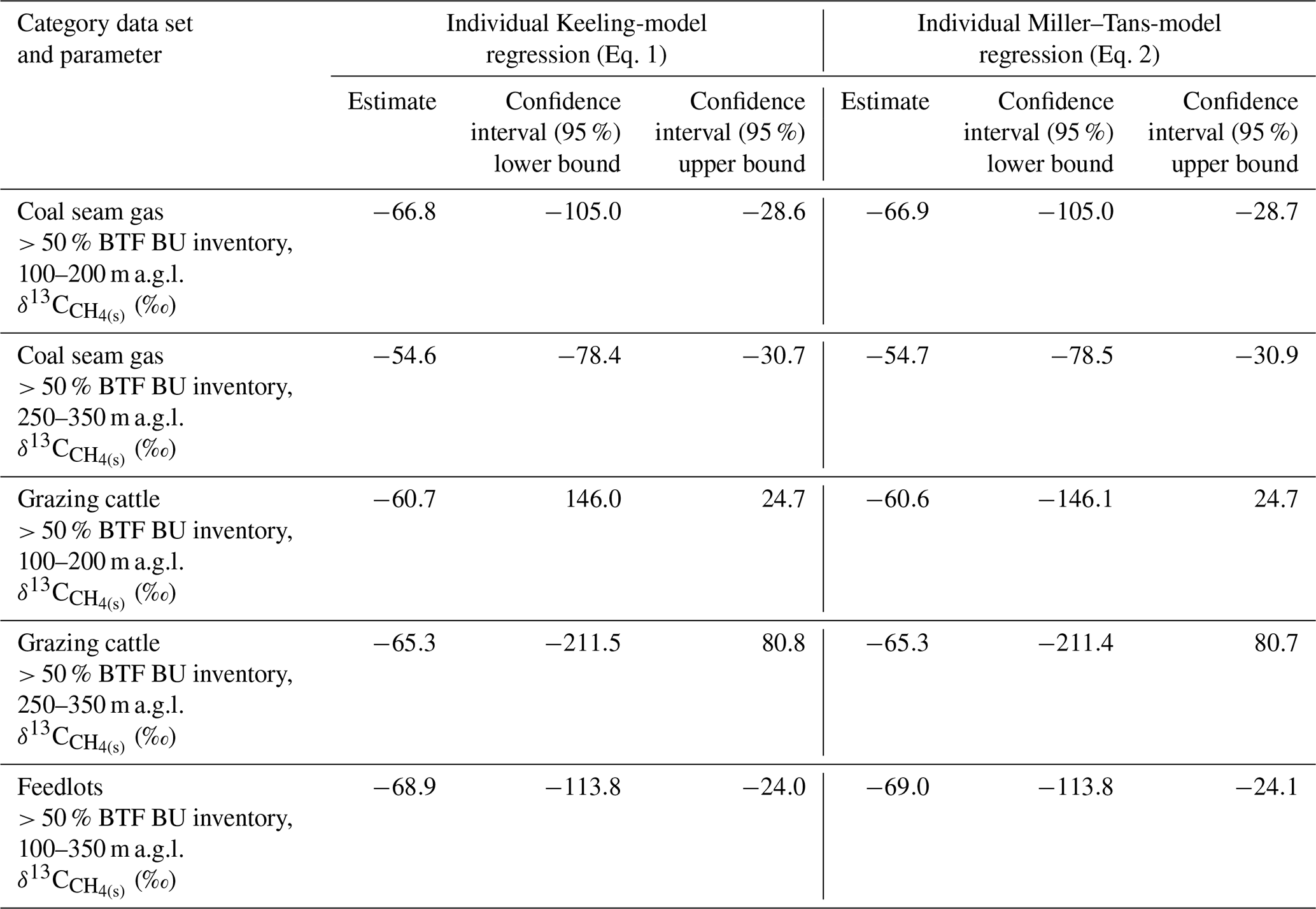
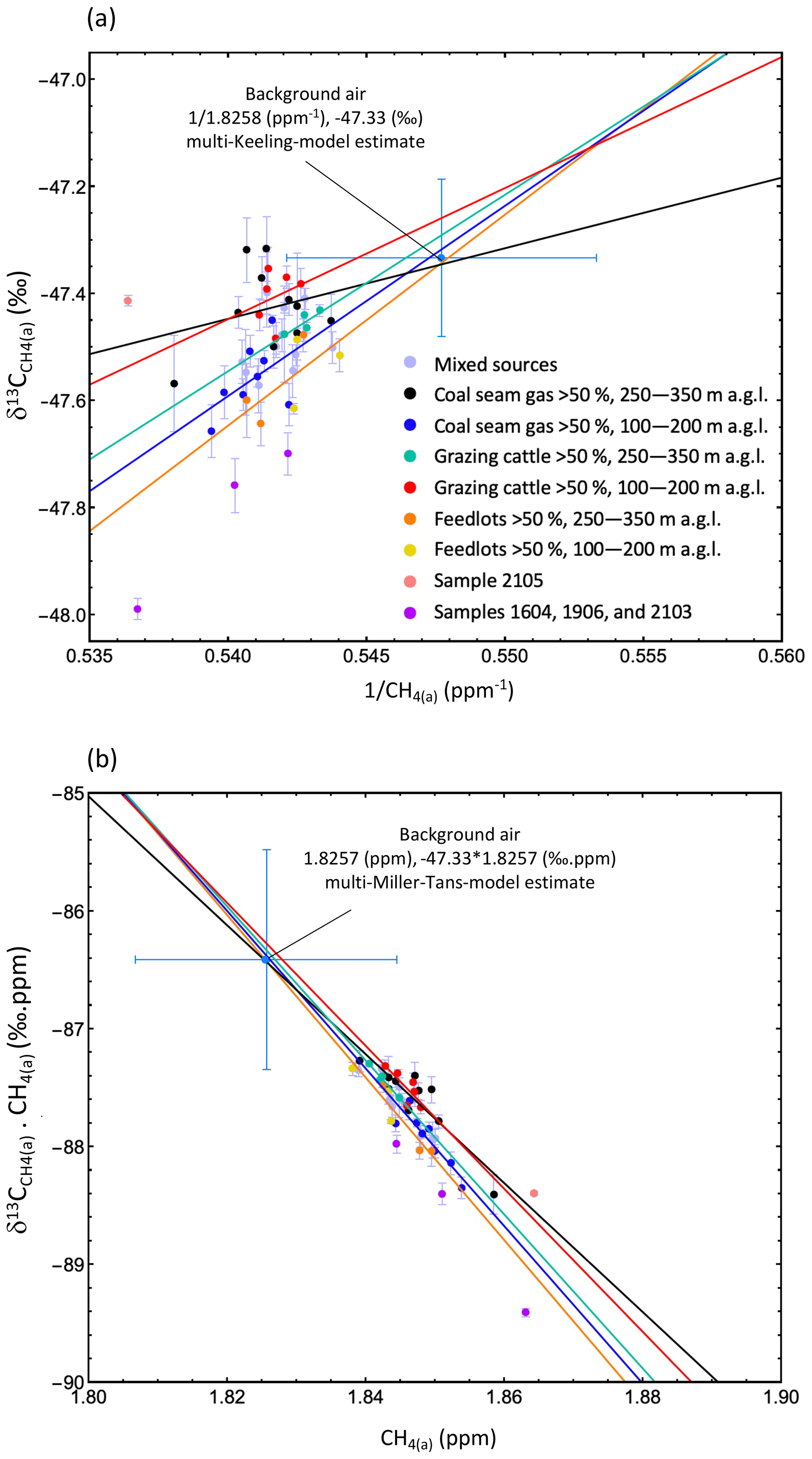
Figure B1Least squares regression for two-endmember mixing models fitted to individual source category data sets using (a) the Keeling model (Eq. 1) and (b) the Miller–Tans model (Eq. 2). For reference the background-air values for CH4(b) and δ13C determined from the multi-Keeling and multi-Miller–Tans-model regressions are displayed in (a) and (b), respectively. The regression statistics for each category are listed in Table B1. Both graphs highlight that when the models are fitted to the individual source category data sets, the lines of best fit do not converge to a common value for background air. All error bars are 1 standard deviation.
The code for the MultiNonlinearModelFit function used in Mathematica (Version 12.0) (Wolfram Research Inc., 2019) is available from the Wolfram function repository (Smit, 1986) (https://resources.wolframcloud.com/FunctionRepository/resources/MultiNonlinearModelFit).
The data used in Figs. 1, 3, 4, 5 and 6 are listed in Tables A2, A3, and A4.
All data sets used for the UNSW inventory in Figs. 2, 7, 8, A1, A2, A3, and A5 are available from Neininger et al. (2021, https://doi.org/10.1098/rsta.2020.0458), their Supplement Sect. S, Tables ST1 to ST7.
BFJK, BGN, JMH, REF, and StS were responsible for project design and securing funding. BGN and JMH collected the air samples. XL, SJH, and BFJK managed the in-field quality assurance testing of the air samples. REF, DL, TR, CvdV, and MM managed and did the laboratory measurements of the air samples. BFJK and XL ran the HYSPLIT calculations and developed and analysed the bottom–up inventory. BFJK conceived the use of multi-Keeling regression and did the regression analyses. XL produced Figs. 1 and 2; all other figures were produced by BFJK. BFJK wrote the paper with the help of XL. BGN, DL, EGN, JLF, REF, SJH, StS, and TR all contributed to the review, additional interpretation, and editing of the paper.
The contact author has declared that none of the authors has any competing interests.
Publisher's note: Copernicus Publications remains neutral with regard to jurisdictional claims in published maps and institutional affiliations.
The authors thank the MSS Science Advisory Committee, the MSS Technical Working Group, and Christopher Konek and Meghan Demeter for their administrative assistance. The authors also thank the UNSW grant management and finance staff. The authors are grateful for the assistance of the staff at the Australian Government, Department of Industry, Science, Energy and Resources, for their guidance on the development of the UNSW inventory. The authors appreciate the constructive feedback from the reviewers, which helped with improving the overall quality of the paper.
Data collection and analysis were funded under the Climate and Clean Air Coalition (CCAC) Oil and Gas Methane Science Studies, hosted by the United Nations Environment Programme (UNEP). Funding was provided by the Environmental Defense Fund, Oil and Gas Climate Initiative, the European Commission, and CCAC. The project funds were managed by The United Nations Environment Programme grant numbers DTIE18-EN067, DTIE19-EN0XX, and DTIE19-EN633 (UNSW grant numbers RG181430 and RG192900). UNSW contributed matching funding via in-kind support for Bryce F. J. Kelly. UNSW researcher Xinyi Lu was partly supported by UNEP. Xinyi Lu was also supported in part by UNSW–China Scholarship Council (CSC). Stephen J. Harris was supported by a Research Training Program scholarship from the Australian Government. Stefan Schwietzke acknowledges additional support from the Robertson Foundation. ARA and MetAir have each contributed about 50 % in kind in accordance with the proposal to UNEP. ARA has been substantially sponsored by the Hackett Foundation in Adelaide. Malika Menoud received funding from the European Union's Horizon 2020 research and innovation programme under the Marie Sklodowska-Curie grant agreement no. 722479, project MEMO2, https://h2020-memo2.eu/ (last access: 8 December 2022).
This paper was edited by Eliza Harris and reviewed by two anonymous referees.
Albers, J. C., Kiers, H. A. L., and van Ravenzwaaij, D.: Credible confidence: a pragmatic view on the frequentist vs Bayesian debate, Collabra: Psychology, 4, 31, https://doi.org/10.1525/collabra.149, 2018.
Australian Competition and Consumer Commission: Gas inquiry 2017–2025 Interim report, https://www.accc.gov.au/publications/serial-publications/gas-inquiry-2017-2025 (last access: 17 January 2022), 2020.
Australian Government: National Inventory Report 2018 Volume 1, https://www.industry.gov.au/data-and-publications/national-greenhouse-gas-inventory-report-2018 (last access: 17 January 2022), 2020a.
Australian Government: Quarterly Update of Australia's National Greenhouse Gas Inventory: September 2020, https://www.industry.gov.au/data-and-publications/national-greenhouse-gas-inventory-quarterly-updates (last access: 17 January 2022), 2020b.
Australian Government: Geoscape Administrative Boundaries, https://data.gov.au/data/dataset/bdcf5b09-89bc-47ec-9281-6b8e9ee147aa, last access: 10 June 2020c.
Australian Government: National Gas Infrastructure Plan, Department of Industry, Science, Energy and Resources, https://www.industry.gov.au/sites/default/files/2022-09/disclosure-log-21-081-70042m.pdf (last access: 8 December 2022), 2021.
Barkley, Z. R., Lauvaux, T., Davis, K. J., Deng, A., Miles, N. L., Richardson, S. J., Cao, Y., Sweeney, C., Karion, A., Smith, M., Kort, E. A., Schwietzke, S., Murphy, T., Cervone, G., Martins, D., and Maasakkers, J. D.: Quantifying methane emissions from natural gas production in north-eastern Pennsylvania, Atmos. Chem. Phys., 17, 13941–13966, https://doi.org/10.5194/acp-17-13941-2017, 2017.
Basu, S., Lan, X., Dlugokencky, E., Michel, S., Schwietzke, S., Miller, J. B., Bruhwiler, L., Oh, Y., Tans, P. P., Apadula, F., Gatti, L. V., Jordan, A., Necki, J., Sasakawa, M., Morimoto, S., Di Iorio, T., Lee, H., Arduini, J., and Manca, G.: Estimating emissions of methane consistent with atmospheric measurements of methane and δ13C of methane, Atmos. Chem. Phys., 22, 15351–15377, https://doi.org/10.5194/acp-22-15351-2022, 2022.
Baublys, K. A., Hamilton, S. K., Golding, S. D., Vink, S., and Esterle, J.: Microbial controls on the origin and evolution of coal seam gases and production waters of the Walloon Subgroup; Surat Basin, Australia, Int. J. Coal Geol., 147–148, 85–104, https://doi.org/10.1016/j.coal.2015.06.007, 2015.
Beck, V., Chen, H., Gerbig, C., Bergamaschi, P., Bruhwiler, L., Houweling, S., Röckmann, T., Kolle, O., Steinbach, J., Koch, T., Sapart, C. J., Veen, C. van der, Frankenberg, C., Andreae, M. O., Artaxo, P., Longo, K. M., and Wofsy, S. C.: Methane airborne measurements and comparison to global models during BARCA, J. Geophys. Res.-Atmos., 117, 15310, https://doi.org/10.1029/2011JD017345, 2012.
Day, C., Tibbett, S., Sestak, A., Knight, S., Marvig, C., Mcgarry, P., Weir, S., White, S., Armand, S., Van Holst, S., Fry, J., Dell'amico, R., Halliburton, M., and Azzi, B.: Methane and Volatile Organic Compound Emissions in New South Wales, https://www.epa.nsw.gov.au/~/media/EPA/Corporate Site/resources/air/methane-volatile-organic-compound-emissions-nsw-3063.ashx (last access: 11 August 2022), 2016.
Desjardins, R. L., Worth, D. E., Pattey, E., VanderZaag, A., Srinivasan, R., Mauder, M., Worthy, D., Sweeney, C., and Metzger, S.: The challenge of reconciling bottom-up agricultural methane emissions inventories with top-down measurements, Agr. Forest Meteorol., 248, 48–59, https://doi.org/10.1016/J.AGRFORMET.2017.09.003, 2018.
Dlugokencky, E. J., Myers, R. C., Lang, P. M., Masarie, K. A., Crotwell, A. M., Thoning, K. W., Hall, B. D., Elkins, J. W., and Steele, L. P.: Conversion of NOAA atmospheric dry air CH4 mole fractions to a gravimetrically prepared standard scale, J. Geophys. Res.-Atmos., 110, 1–8, https://doi.org/10.1029/2005JD006035, 2005.
Draper, J. J. and Boreham, C. J.: Geological Controls On Exploitable Coal Seam Gas Distribution In Queensland, APPEA J., 46, 366, https://doi.org/10.1071/aj05019, 2006.
Draxler, R. R., Spring, S., Maryland, U. S. A., and Hess, G. D.: An Overview of the HYSPLIT_4 Modelling System for Trajectories, Dispersion, and Deposition, Aust. Meteorol. Mag., 47, 295–308, 1998.
EFDB: Change, Emission Factor Database EFDB, IPCC – Intergovernmental Panel on Climate, https://www.ipcc-nggip.iges.or.jp/EFDB/main.php (last access: 23 August 2021), 2006.
Fisher, R., Lowry, D., Wilkin, O., Sriskantharajah, S., and Nisbet, E. G.: High-precision, automated stable isotope analysis of atmospheric methane and carbon dioxide using continuous-flow isotope-ratio mass spectrometry, Rapid Commun. Mass Spectrom., 20, 200–208, https://doi.org/10.1002/rcm.2300, 2006.
Fisher, R. E., France, J. L., Lowry, D., Lanoisellé, M., Brownlow, R., Pyle, J. A., Cain, M., Warwick, N., Skiba, U. M., Drewer, J., Dinsmore, K. J., Leeson, S. R., Bauguitte, S. J.-B., Wellpott, A., O'Shea, S. J., Allen, G., Gallagher, M. W., Pitt, J., Percival, C. J., Bower, K., George, C., Hayman, G. D., Aalto, T., Lohila, A., Aurela, M., Laurila, T., Crill, P. M., McCalley, C. K., and Nisbet, E. G.: Measurement of the 13C isotopic signature of methane emissions from northern European wetlands, Global Biogeochem. Cy., 31, 605–623, https://doi.org/10.1002/2016GB005504, 2017.
France, J. L., Cain, M., Fisher, R. E., Lowry, D., Allen, G., O'Shea, S. J., Illingworth, S., Pyle, J., Warwick, N., Jones, B. T., Gallagher, M. W., Bower, K., Le Breton, M., Percival, C., Muller, J., Welpott, A., Bauguitte, S., George, C., Hayman, G. D., Manning, A. J., Myhre, C. L., Lanoisellé, M., and Nisbet, E. G.: Measurements of δ13C in CH4 and using particle dispersion modeling to characterize sources of Arctic methane within an air mass, J. Geophys. Res.-Atmos., 121, 14257–14270, https://doi.org/10.1002/2016JD026006, 2016.
France, J. L., Bateson, P., Dominutti, P., Allen, G., Andrews, S., Bauguitte, S., Coleman, M., Lachlan-Cope, T., Fisher, R. E., Huang, L., Jones, A. E., Lee, J., Lowry, D., Pitt, J., Purvis, R., Pyle, J., Shaw, J., Warwick, N., Weiss, A., Wilde, S., Witherstone, J., and Young, S.: Facility level measurement of offshore oil and gas installations from a medium-sized airborne platform: method development for quantification and source identification of methane emissions, Atmos. Meas. Tech., 14, 71–88, https://doi.org/10.5194/amt-14-71-2021, 2021.
Ginty, E. M.: Carbon Isotopic Evidence That Coal Derived Methane Is Altering The Chemistry of The Global Atmosphere, Honours thesis, The University of New South Wales, Australia, 63 pp., 2016.
Godwin, S., Kang, A., Gulino, L.-M., Manefield, M., Gutierrez-Zamora, M.-L., Kienzle, M., Ouwerkerk, D., Dawson, K., and Klieve, A. V: Investigation of the microbial metabolism of carbon dioxide and hydrogen in the kangaroo foregut by stable isotope probing, ISME J., 89, 1855–1865, https://doi.org/10.1038/ismej.2014.25, 2014.
Gorchov Negron, A. M., Kort, E. A., Conley, S. A., and Smith, M. L.: Airborne Assessment of Methane Emissions from Offshore Platforms in the U.S. Gulf of Mexico, Environ. Sci. Technol., 54, 5112–5120, https://doi.org/10.1021/acs.est.0c00179, 2020.
Hamilton, S. K., Esterle, J. S., and Golding, S. D.: Geological interpretation of gas content trends, Walloon Subgroup, eastern Surat Basin, Queensland, Australia, Int. J. Coal Geol., 101, 21–35, https://doi.org/10.1016/j.coal.2012.07.001, 2012.
Hamilton, S. K., Golding, S. D., Baublys, K. A., and Esterle, J. S.: Stable isotopic and molecular composition of desorbed coal seam gases from the Walloon Subgroup, eastern Surat Basin, Australia, Int. J. Coal Geol., 122, 21–36, https://doi.org/10.1016/j.coal.2013.12.003, 2014.
Hamilton, S. K., Golding, S. D., Baublys, K. A., and Esterle, J. S.: Conceptual exploration targeting for microbially enhanced coal bed methane (MECoM) in the Walloon Subgroup, eastern Surat Basin, Australia, Int. J. Coal Geol., 138, 68–82, https://doi.org/10.1016/j.coal.2014.12.002, 2015.
Han, P., Zeng, N., Oda, T., Lin, X., Crippa, M., Guan, D., Janssens-Maenhout, G., Ma, X., Liu, Z., Shan, Y., Tao, S., Wang, H., Wang, R., Wu, L., Yun, X., Zhang, Q., Zhao, F., and Zheng, B.: Evaluating China's fossil-fuel CO2 emissions from a comprehensive dataset of nine inventories, Atmos. Chem. Phys., 20, 11371–11385, https://doi.org/10.5194/acp-20-11371-2020, 2020.
IPCC: Guidelines for National Greenhouse Gas Inventories (NGHGI), https://www.ipcc-nggip.iges.or.jp/public/2006gl/index.html (last access: 23 August 2021), 2006.
IPCC: Refinement to the 2006 IPCC Guidelines for National Greenhouse Gas Inventories, https://www.ipcc.ch/report/2019-refinement-to-the-2006-ipcc-guidelines-for-national-greenhouse-gas-inventories/ (last access: 23 August 2021), 2019.
Iverach, C. P., Cendón, D. I., Hankin, S. I., Lowry, D., Fisher, R. E., France, J. L., Nisbet, E. G., Baker, A., and Kelly, B. F. J.: Assessing Connectivity Between an Overlying Aquifer and a Coal Seam Gas Resource Using Methane Isotopes, Dissolved Organic Carbon and Tritium, Sci. Rep.-UK, 5, 1–11, https://doi.org/10.1038/srep15996, 2015.
Iverach, C. P., Beckmann, S., Cendón, D. I., Manefield, M., and Kelly, B. F. J.: Biogeochemical constraints on the origin of methane in an alluvial aquifer: evidence for the upward migration of methane from underlying coal measures, Biogeosciences, 14, 215–228, https://doi.org/10.5194/bg-14-215-2017, 2017.
Jemena: Darling Downs Pipeline, https://jemena.com.au/pipelines/darling-downs-pipeline, last access: 29 August 2021.
Johnson, M. R., Tyner, D. R., Conley, S., Schwietzke, S., and Zavala-Araiza D.: Comparisons of airborne measurements and inventory estimates of methane emissions in the Alberta upstream oil and gas sector, Environ. Sci. Technol., 51, 13008–13017, https://doi.org/10.1021/acs.est.7b03525, 2017.
Karion, A., Sweeney, C., Pétron, G., Frost, G., Michael Hardesty, R., Kofler, J., Miller, B. R., Newberger, T., Wolter, S., Banta, R., Brewer, A., Dlugokencky, E., Lang, P., Montzka, S. A., Schnell, R., Tans, P., Trainer, M., Zamora, R., and Conley, S.: Methane emissions estimate from airborne measurements over a western United States natural gas field, Geophys. Res. Lett., 40, 4393–4397, https://doi.org/10.1002/grl.50811, 2013.
Karion, A., Sweeney, C., Kort, E. A., Shepson, P. B., Brewer, A., Cambaliza, M., Conley, S. A., Davis, K., Deng, A., Hardesty, M., Herndon, S. C., Lauvaux, T., Lavoie, T., Lyon, D., Newberger, T., Pétron, G., Rella, C., Smith, M., Wolter, S., Yacovitch, T. I., and Tans, P.: Aircraft-Based Estimate of Total Methane Emissions from the Barnett Shale Region, Environ. Sci. Technol., 49, 8124–8131, https://doi.org/10.1021/acs.est.5b00217, 2015.
Keeling, C. D.: The concentration and isotopic abundances of carbon dioxide in rural and marine air, Geochim. Cosmochim. Ac., 24, 277–298, https://doi.org/10.1016/0016-7037(61)90023-0, 1961.
Kirschke, S., Bousquet, P., Ciais, P., Saunois, M., Canadell, J. G., Dlugokencky, E. J., Bergamaschi, P., Bergmann, D., Blake, D. R., Bruhwiler, L., Cameron-Smith, P., Castaldi, S., Chevallier, F., Feng, L., Fraser, A., Heimann, M., Hodson, E. L., Houweling, S., Josse, B., Fraser, P. J., Krummel, P. B., Lamarque, J.-F., Langenfelds, R. L., Le Quéré, C., Naik, V., Palmer, P. I., Pison, I., Plummer, D., Poulter, B., Prinn, R. G., Rigby, M., Ringeval, B., Santini, M., Schmidt, M., Shindell, D. T., Simpson, I. J., Spahni, R., Paul Steele, L., Strode, S. A., Sudo, K., Szopa, S., van der Werf, G. R., Voulgarakis, A., van Weele, M., Weiss, R. F., Williams, J. E., and Zeng, G.: Three decades of global methane sources and sinks, Nat. Geosci., 6, 813–823, https://doi.org/10.1038/NGEO1955, 2013.
Lan, X., Basu, S., Schwietzke, S., Bruhwiler, L. M. P., Dlugokencky, E. J., Michel, S. E., Sherwood, O. A., Tans, P. P., Thoning, K., Etiope, G., Zhuang, Q., Liu, L., Oh, Y., Miller, J. B., Pétron, G., Vaughn, B. H., and Crippa, M.: Improved Constraints on Global Methane Emissions and Sinks Using δ13C-CH4, Global Biogeochem. Cy., 35, e2021GB007000, https://doi.org/10.1029/2021GB007000, 2021.
Lowry, D., Fisher, R. E., France, J. L., Coleman, M., Lanoisellé, M., Zazzeri, G., Nisbet, E. G., Shaw, J. T., Allen, G., Pitt, J., and Ward, R. S.: Environmental baseline monitoring for shale gas development in the UK: Identification and geochemical characterisation of local source emissions of methane to atmosphere, Sci. Total Environ., 708, 134600, https://doi.org/10.1016/j.scitotenv.2019.134600, 2020.
Lu, D., Ye., M., and Hill, M. C.: Analysis of regression confidence intervals and Bayesian credible intervals for uncertainty quantification, Water Resour. Res., 48, W09521, https://doi.org/10.1029/2011WR011289, 2012.
Lu, X., Harris, S. J., Fisher, R. E., France, J. L., Nisbet, E. G., Lowry, D., Röckmann, T., van der Veen, C., Menoud, M., Schwietzke, S., and Kelly, B. F. J.: Isotopic signatures of major methane sources in the coal seam gas fields and adjacent agricultural districts, Queensland, Australia, Atmos. Chem. Phys., 21, 10527–10555, https://doi.org/10.5194/acp-21-10527-2021, 2021.
Menoud, M., van der Veen, C., Scheeren, B., Chen, H., Szénási, B., Morales, R. P., Pison, I., Bousquet, P., Brunner, D., and Röckmann, T.: Characterisation of methane sources in Lutjewad, The Netherlands, using quasi-continuous isotopic composition measurements, Tellus B, 72, 1–19, https://doi.org/10.1080/16000889.2020.1823733, 2020.
Menoud, M., van der Veen, C., Necki, J., Bartyzel, J., Szénási, B., Stanisavljević, M., Pison, I., Bousquet, P., and Röckmann, T.: Methane (CH4) sources in Krakow, Poland: insights from isotope analysis, Atmos. Chem. Phys., 21, 13167–13185, https://doi.org/10.5194/acp-21-13167-2021, 2021.
Menoud, M., van der Veen, C., Lowry, D., Fernandez, J. M., Bakkaloglu, S., France, J. L., Fisher, R. E., Maazallahi, H., Stanisavljević, M., Nȩcki, J., Vinkovic, K., Łakomiec, P., Rinne, J., Korbeń, P., Schmidt, M., Defratyka, S., Yver-Kwok, C., Andersen, T., Chen, H., and Röckmann, T.: New contributions of measurements in Europe to the global inventory of the stable isotopic composition of methane, Earth Syst. Sci. Data, 14, 4365–4386, https://doi.org/10.5194/essd-14-4365-2022, 2022a.
Menoud, M., van der Veen, C., Maazallahi, H., Hensen, A., Velzeboer, I., van den Bulk, P., Delre, A., Korben, P., Schwietzke, S., Ardelean, M., Calcan, A., Etiope, G., Baciu, C., Scheutz, C., Schmidt, M., and Röckmann, T.: CH4 isotopic signatures of emissions from oil and gas extraction sites in Romania, Elementa, 10, 00092, https://doi.org/10.1525/elementa.2021.00092, 2022b.
Mielke-Maday, I., Schwietzke, S., Yacovitch, T.I., Miller, B., Conley, S., Kofler, J., Handley, P., Thorley, E., Herndon, S. C., Hall, B., Dlugokencky, E., Lang, P., Wolter, S., Moglia, E., Crotwell, M., Crotwell, A., Rhodes, M., Kitzis, D., Vaughn, T., Bell, C., Zimmerle, D., Schnell, R., and Pétron G.: Methane source attribution in a U.S. dry gas basin using spatial patterns of ground and airborne ethane and methane measurements, Elementa, 7, 351, https://doi.org/10.1525/elementa.351, 2019.
Milkov, A. V. and Etiope, G.: Revised genetic diagrams for natural gases based on a global dataset of > 20,000 samples, Org. Geochem., 125, 109–120, https://doi.org/10.1016/J.ORGGEOCHEM.2018.09.002, 2018.
Miller, J. B. and Tans, P. P.: Calculating isotopic fractionation from atmospheric measurements at various scales, Tellus B, 55, 207–214, https://doi.org/10.1034/j.1600-0889.2003.00020.x, 2003.
Neininger, B. G., Kelly, B. F. J., Hacker, J. M., Lu, X., and Schwietzke, S.: Coal seam gas industry methane emissions in the Surat Basin, Australia: Comparing airborne measurements with inventories, Philos. T. R. Soc. A, 379, 20200458, https://doi.org/10.1098/rsta.2020.0458, 2021.
Pataki, D. E., Ehleringer, J. R., Flanagan, L. B., Yakir, D., Bowling, D. R., Still, C. J., Buchmann, N., Kaplan, J. O., and Berry, J. A.: The application and interpretation of Keeling plots in terrestrial carbon cycle research, Global Biogeochem. Cy., 17, 1022, https://doi.org/10.1029/2001GB001850, 2003.
Peischl, J., Ryerson, T. B., Aikin, K. C., De Gouw, J. A., Gilman, J. B., Holloway, J. S., Lerner, B. M., Nadkarni, R., Neuman, J. A., Nowak, J. B., Trainer, M., Warneke, C., and Parrish, D. D.: Quantifying atmospheric methane emissions from the Haynesville, Fayetteville, and northeastern Marcellus shale gas production regions, J. Geophys. Res., 120, 2119–2139, https://doi.org/10.1002/2014JD022697, 2015.
Peischl, J., Karion, A., Sweeney, C., Kort, E. A., Smith, M. L., Brandt, A. R., Yeskoo, T., Aikin, K. C., Conley, S. A., Gvakharia, A., Trainer, M., Wolter, S., and Ryerson, T. B.: Quantifying atmospheric methane emissions from oil and natural gas production in the Bakken shale region of North Dakota, J. Geophys. Res.-Atmos., 121, 6101–6111, https://doi.org/10.1002/2015JD024631, 2016.
Peischl, J., Eilerman, S. J., Neuman, J. A., Aikin, K. C., de Gouw, J., Gilman, J. B., Herndon, S. C., Nadkarni, R., Trainer, M., Warneke, C., and Ryerson, T. B.: Quantifying Methane and Ethane Emissions to the Atmosphere From Central and Western U.S. Oil and Natural Gas Production Regions, J. Geophys. Res.-Atmos., 123, 7725–7740, https://doi.org/10.1029/2018JD028622, 2018.
Pétron, G., Karion, A., Sweeney, C., Miller, B. R., Montzka, S. A., Frost, G. J., Trainer, M., Tans, P., Andrews, A., Kofler, J., Helmig, D., Guenther, D., Dlugokencky, E., Lang, P., Newberger, T., Wolter, S., Hall, B., Novelli, P., Brewer, A., Conley, S., Hardesty, M., Banta, R., White, A., Noone, D., Wolfe, D., and Schnell, R.: A new look at methane and nonmethane hydrocarbon emissions from oil and natural gas operations in the Colorado Denver-Julesburg Basin, J. Geophys. Res., 119, 6836–6852, https://doi.org/10.1002/2013JD021272, 2014.
QGC: Surat North Development Water Resource Monitoring and Management Plan, Stage 3 Water Monitoring and Management Plane, Chapter 14: Associated Water Management, https://www.shell.com.au/about-us/projects-and-locations/qgc/environment/water-management/reports.html (last access: 27 February 2022), 2013.
Quay, P., Stutsman, J., Wilbur, D., Snover, A., Dlugokencky, E., and Brown, T.: The isotopic composition of atmospheric methane, Global Biogeochem. Cy., 13, 445–461, https://doi.org/10.1029/1998GB900006, 1999.
Röckmann, T., Eyer, S., van der Veen, C., Popa, M. E., Tuzson, B., Monteil, G., Houweling, S., Harris, E., Brunner, D., Fischer, H., Zazzeri, G., Lowry, D., Nisbet, E. G., Brand, W. A., Necki, J. M., Emmenegger, L., and Mohn, J.: In situ observations of the isotopic composition of methane at the Cabauw tall tower site, Atmos. Chem. Phys., 16, 10469–10487, https://doi.org/10.5194/acp-16-10469-2016, 2016.
Saunois, M., Stavert, A. R., Poulter, B., Bousquet, P., Canadell, J. G., Jackson, R. B., Raymond, P. A., Dlugokencky, E. J., Houweling, S., Patra, P. K., Ciais, P., Arora, V. K., Bastviken, D., Bergamaschi, P., Blake, D. R., Brailsford, G., Bruhwiler, L., Carlson, K. M., Carrol, M., Castaldi, S., Chandra, N., Crevoisier, C., Crill, P. M., Covey, K., Curry, C. L., Etiope, G., Frankenberg, C., Gedney, N., Hegglin, M. I., Höglund-Isaksson, L., Hugelius, G., Ishizawa, M., Ito, A., Janssens-Maenhout, G., Jensen, K. M., Joos, F., Kleinen, T., Krummel, P. B., Langenfelds, R. L., Laruelle, G. G., Liu, L., Machida, T., Maksyutov, S., McDonald, K. C., McNorton, J., Miller, P. A., Melton, J. R., Morino, I., Müller, J., Murguia-Flores, F., Naik, V., Niwa, Y., Noce, S., O'Doherty, S., Parker, R. J., Peng, C., Peng, S., Peters, G. P., Prigent, C., Prinn, R., Ramonet, M., Regnier, P., Riley, W. J., Rosentreter, J. A., Segers, A., Simpson, I. J., Shi, H., Smith, S. J., Steele, L. P., Thornton, B. F., Tian, H., Tohjima, Y., Tubiello, F. N., Tsuruta, A., Viovy, N., Voulgarakis, A., Weber, T. S., van Weele, M., van der Werf, G. R., Weiss, R. F., Worthy, D., Wunch, D., Yin, Y., Yoshida, Y., Zhang, W., Zhang, Z., Zhao, Y., Zheng, B., Zhu, Q., Zhu, Q., and Zhuang, Q.: The Global Methane Budget 2000–2017, Earth Syst. Sci. Data, 12, 1561–1623, https://doi.org/10.5194/essd-12-1561-2020, 2020.
Schwietzke, S., Pétron, G., Conley, S., Pickering, C., Mielke-Maday, I., Dlugokencky, E. J., Tans, P. P., Vaughn, T., Bell, C., Zimmerle, D., Wolter, S., King, C. W., White, A. B., Coleman, T., Bianco, L., and Schnell, R. C.: Improved Mechanistic Understanding of Natural Gas Methane Emissions from Spatially Resolved Aircraft Measurements, Environ. Sci. Technol., 51, 7286–7294, https://doi.org/10.1021/acs.est.7b01810, 2017.
Scott, S., Anderson, B., Crosdale, P., Dingwall, J., and Leblang, G.: Coal petrology and coal seam gas contents of the Walloon Subgroup – Surat Basin, Queensland, Australia, Int. J. Coal Geol., 70, 209–222, https://doi.org/10.1016/J.COAL.2006.04.010, 2007.
Sherwood, O. A., Schwietzke, S., Arling, V. A., and Etiope, G.: Global Inventory of Gas Geochemistry Data from Fossil Fuel, Microbial and Burning Sources, version 2017, Earth Syst. Sci. Data, 9, 639–656, https://doi.org/10.5194/essd-9-639-2017, 2017.
Sherwood, O. A., Schwietzke, S., and Lan, X.: NOAA Global Monitoring Laboratory Data Repository, Global δ13C-CH4, Source Signature Inventory 2020, https://doi.org/10.15138/qn55-e011, 2020.
Smit, S.: MultiNonlinearModelFit, Wolfram Function Repository [code], https://resources.wolframcloud.com/FunctionRepository/resources/MultiNonlinearModelFit (last access: 27 January 2022), 1986.
Smith, M. L., Kort, E. A., Karion, A., Sweeney, C., Herndon, S. C., and Yacovitch, T. I.: Airborne ethane observations in the Barnett Shale: quantification of ethane flux and attribution of methane emissions, Environ. Sci. Technol., 49, 8158–8166, https://doi.org/10.1021/acs.est.5b00219, 2015.
Stein, A. F., Draxler, R. R., Rolph, G. D., Stunder, B. J. B., Cohen, M. D., and Ngan, F.: NOAA's HYSPLIT Atmospheric Transport and Dispersion Modeling System, B. Am. Meteorol. Soc., 96, 2059–2077, https://doi.org/10.1175/BAMS-D-14-00110.1, 2015.
Sugimoto, A., Inoue, T., Tayasu, I., Miller, L., Takeichi, S., and Abe, T.: Methane and hydrogen production in a termite-symbiont system, Ecol. Res., 13, 241–257, https://doi.org/10.1046/j.1440-1703.1998.00262.x, 1998.
Tarasova, O. A., Brenninkmeijer, C. A. M., Assonov, S. S., Elansky, N. F., Röckmann, T., and Brass, M.: Atmospheric CH4 along the Trans-Siberian railroad (TROICA) and river Ob: Source identification using stable isotope analysis, Atmos. Environ., 40, 5617–5628, https://doi.org/10.1016/j.atmosenv.2006.04.065, 2006.
Townsend-Small, A., Marrero, J. E., Lyon, D. R., Simpson, I. J., Meinardi, S., and Blake, D. R.: Integrating Source Apportionment Tracers into a Bottom-up Inventory of Methane Emissions in the Barnett Shale Hydraulic Fracturing Region, Environ. Sci. Technol., 49, 8175–8182, https://doi.org/10.1021/acs.est.5b00057, 2015.
Turner, A. J., Jacob, D. J., Wecht, K. J., Maasakkers, J. D., Lundgren, E., Andrews, A. E., Biraud, S. C., Boesch, H., Bowman, K. W., Deutscher, N. M., Dubey, M. K., Griffith, D. W. T., Hase, F., Kuze, A., Notholt, J., Ohyama, H., Parker, R., Payne, V. H., Sussmann, R., Sweeney, C., Velazco, V. A., Warneke, T., Wennberg, P. O., and Wunch, D.: Estimating global and North American methane emissions with high spatial resolution using GOSAT satellite data, Atmos. Chem. Phys., 15, 7049–7069, https://doi.org/10.5194/acp-15-7049-2015, 2015.
Vardag, S. N., Hammer, S., and Levin, I.: Evaluation of 4 years of continuous δ13C(CO2) data using a moving Keeling plot method, Biogeosciences, 13, 4237–4251, https://doi.org/10.5194/bg-13-4237-2016, 2016.
Verhulst, K. R., Karion, A., Kim, J., Salameh, P. K., Keeling, R. F., Newman, S., Miller, J., Sloop, C., Pongetti, T., Rao, P., Wong, C., Hopkins, F. M., Yadav, V., Weiss, R. F., Duren, R. M., and Miller, C. E.: Carbon dioxide and methane measurements from the Los Angeles Megacity Carbon Project – Part 1: calibration, urban enhancements, and uncertainty estimates, Atmos. Chem. Phys., 17, 8313–8341, https://doi.org/10.5194/acp-17-8313-2017, 2017.
Whiticar, M. J.: Carbon and hydrogen isotope systematics of bacterial formation and oxidation of methane, Chem. Geol., 161, 291–314, https://doi.org/10.1016/S0009-2541(99)00092-3, 1999.
WMO: GAW Report No. 255, 20th WMO/IAEA Meeting on Carbon Dioxide, Other Greenhouse Gases and Related Measurement Techniques (GGMT-2019), Jeju Island, South Korea, https://library.wmo.int/doc_num.php?explnum_id=10353 (last access: 9 April 2021), 2020.
Wolfram Research Inc.: Mathematica Version 12.0, Champaign, Illinois, https://www.wolfram.com/mathematica (last access: 17 January 2022), 2019.
Worden, J. R., Bloom, A. A., Pandey, S., Jiang, Z., Worden, H. M., Walker, T. W., Houweling, S., and Röckmann, T.: Reduced biomass burning emissions reconcile conflicting estimates of the post-2006 atmospheric methane budget, Nat. Commun., 8, 1–11, https://doi.org/10.1038/s41467-017-02246-0, 2017.
Yacovitch, T. I., Neininger, B., Herndon, S. C., van der Gon, H. D., Jonkers, S., Hulskotte, J., Roscioli, J. R., and Zavala-Araiza, D.: Methane emissions in the Netherlands: The Groningen field, Elementa, 6, 57, https://doi.org/10.1525/ELEMENTA.308, 2018.
Zazzeri, G., Lowry, D., Fisher, R. E., France, J. L., Lanoisellé, M., Grimmond, C. S. B., and Nisbet, E. G.: Evaluating methane inventories by isotopic analysis in the London region, Sci. Rep.-UK, 7, 4854, https://doi.org/10.1038/S41598-017-04802-6, 2017.
Zhang, Y., Gautam, R., Pandey, S., Omara, M., Maasakkers, J. D., Sadavarte, P., Lyon, D., Nesser, H., Sulprizio, M. P., Varon, D. J., Zhang, R., Houweling, S., Zavala-Araiza, D., Alvarez, R. A., Lorente, A., Hamburg, S. P., Aben, I., and Jacob, D. J.: Quantifying methane emissions from the largest oil-producing basin in the United States from space, Sci. Adv., 6, 1–10, https://doi.org/10.1126/sciadv.aaz5120, 2020.
Zhang, Y., Jacob, D. J., Lu, X., Maasakkers, J. D., Scarpelli, T. R., Sheng, J.-X., Shen, L., Qu, Z., Sulprizio, M. P., Chang, J., Bloom, A. A., Ma, S., Worden, J., Parker, R. J., and Boesch, H.: Attribution of the accelerating increase in atmospheric methane during 2010–2018 by inverse analysis of GOSAT observations, Atmos. Chem. Phys., 21, 3643–3666, https://doi.org/10.5194/acp-21-3643-2021, 2021.