The historical ozone trends simulated with the SOCOLv4 and their comparison with observations and reanalyses

There is evidence that the ozone layer has begun to recover owing to the ban on the production of halogenated ozone-depleting substances (hODS) accomplished by the Montreal Protocol and its amendments and adjustments (MPA). However, recent studies, while reporting an increase in tropospheric ozone from the anthropogenic NO_x and CH₄ and confirming the ozone recovery in the upper stratosphere from the effects of hODS, also indicate a continuing decline in the lower tropical and mid-latitudinal stratospheric ozone. While these are indications derived from observations, they are not reproduced by current global chemistry–climate models (CCMs), which show positive or near-zero trends for ozone in the lower stratosphere. This makes it difficult to robustly establish ozone evolution and has sparked debate about the ability of contemporary CCMs to simulate future ozone trends. We applied the new Earth system model (ESM) SOCOLv4 (SOlar Climate Ozone Links, version 4) to calculate long-term ozone trends between 1985–2018 and compare them with trends derived from the BAyeSian Integrated and Consolidated (BASIC) ozone composite and MERRA-2, ERA-5, and MSRv2 reanalyses. We designed the model experiment with a six-member ensemble to account for the uncertainty of the natural variability. The trend analysis is performed separately for the ozone depletion (1985–1997) and ozone recovery (1998–2018) phases of the ozone evolution. Within the 1998–2018 period, SOCOLv4 shows statistically significant positive ozone trends in the mesosphere, upper and middle stratosphere, and a steady increase in the tropospheric ozone. The SOCOLv4 results also suggest slightly negative trends in the extra-polar lower stratosphere, yet they barely agree with the BASIC ozone composite in terms of magnitude and statistical significance. However, in some realizations of the SOCOLv4 experiment, the pattern of ozone trends in the lower stratosphere resembles much of what is observed, suggesting that SOCOLv4 may be able to reproduce the observed trends in this region. Thus, the model results reveal marginally significant negative ozone changes in parts of the low-latitude lower stratosphere, which agrees in general with the negative tendencies extracted from the satellite data composite. Despite the slightly smaller significance and magnitude of the simulated ensemble mean, we confirm that modern CCMs such as SOCOLv4 are generally capable of simulating the observed ozone changes, justifying their use to project the future evolution of the ozone layer.

1 Introduction

There is evidence that the restrictions on halogenated ozone-depleting substances (hODS) introduced by the Montreal Protocol and its amendments and adjustments (MPA) have clearly taken effect over the past 25 years, leading to observable ozone increases at certain latitudes and altitudes (WMO, 2014, 2018; McKenzie et al., 2019). The positive role of MPA has also been confirmed by model simulations of ozone depletion under the “world-avoided” scenario (Newman et al., 2009; Garcia et al., 2012; Egorova et al., 2013; Goyal et al., 2019). Using the future simulation of multiple chemistry–climate models (CCMs), Dhomse et al. (2018) estimated the approximate time of the return of ozone concentrations to pre-1980 levels for different regions, again highlighting the success of MPA in protecting ozone.

In the mid-to-late 1990s, the mixing rations of hODS reached their maximum and thereafter started dropping again by virtue of the MPA. The annual mean total column ozone (TOTOZ) in the mid-1990s is quantified to be about 5 % below its pre-1960 level globally, and about 17 % lower over Antarctica (WMO, 2018). Since the turn of the century, total ozone has been expected to increase, but given the long lifetimes of some hODS and the simultaneously changing climate, it is not easy to project how long it will take for ozone to return to the natural pre-1960 level. The near-global TOTOZ (stratospheric plus tropospheric) remained stable since 2000, showing no or a slightly positive trend, albeit statistically not significant (WMO, 2014, 2018; Ball et al., 2018). Nonetheless, ozone concentrations are expected to exceed the pre-ozone hole level in the mid- and high latitudes because of the increasing greenhouse gas (GHG) concentrations (WMO, 2010).

Although the evolution of the TOTOZ is well studied, the evolution of ozone in different atmospheric layers has its own characteristics. For instance, in the troposphere, the ozone concentration has been continuously increasing (Mickley et al., 2001) due to the continuous enhancement in tropospheric ozone precursors, mainly NO_x and CO (Griffiths et al., 2021). Hence, a positive trend in tropospheric ozone is expected (Ziemke et al., 2019). At the same time, simulating the evolution of tropospheric ozone remains challenging because its changes depend on complex, interdependent interactions among precursor emissions, atmospheric transport, photochemical production, deposition, and stratosphere–troposphere exchange. Recent results indicate that models cannot properly capture the tropospheric ozone trends and that tropospheric ozone variability diverges widely among models (Parrish et al., 2014; Revell et al., 2018; Zhang and Cui, 2022).

In the upper stratosphere (above 10 hPa), the ozone abundance declined by about 4 %–8 % between 1980 to the late 1990s due to a continuous increase in stratospheric chlorine loading (e.g., Steinbrecht et al., 2017; WMO, 2018), but since the late 1990s, it has been increasing steadily (Ball et al., 2018; WMO, 2018). The positive trends in ozone in the upper stratosphere are statistically robust according to various analyses of satellite observations and model simulations (Harris et al., 2015; Steinbrecht et al., 2017; Ball et al., 2018; Godin-Beekmann et al., 2022).The main driver of the upper stratospheric ozone increase is the reduction of halogen loading. In addition, the temperature decrease caused by increases in greenhouse gases (GHGs), primarily CO₂, slows down the temperature-dependent catalytic ozone depletion cycles (Hitchman and Brasseur, 1988; Zubov et al., 2013; WMO, 2018). Via the reaction CH₄ + Cl → CH₃ + HCl, the increase in CH₄ further promotes the enhancement of the ozone layer in the upper stratosphere (Hitchman and Brasseur, 1988). It should be noted that not all GHGs (like CO₂ or CH₄) contribute to increases in ozone concentrations and, for instance, N₂O is expected to be the most important anthropogenic compound that will delay the return of ozone to the pre-1960 level (Chipperfield, 2009).

Lower stratospheric ozone (LSO) has increased more slowly than expected, if at all, despite its recovery from the effects of hODS (Ball et al., 2018, 2019). Ball et al. (2018) based their analysis on dynamical linear regression modeling (DLM), a class of non-stationary time-series models which are the next generation of multiple linear regression (MLR) that considers the level of trend non-linearity, thereby increasing the accuracy of the estimate. Ball et al. (2018) applied DLM to the homogenized BAyeSian Integrated and Consolidated (BASIC) composite ozone time series, which was derived from satellite observations (Ball et al., 2017). Using partial ozone columns, a statistically robust negative tendency was found for the layer between 146 and 32 hPa on the near-global scale (55^∘ N–55^∘ S). Ball et al. (2018) reasoned that the detection of this negative trend in LSO was previously prevented by not properly excluding the contribution from increasing tropospheric ozone, which partially compensates for the negative LSO changes in TOTOZ analyses (Ziemke et al., 2019). The results of Ball et al. (2018) have sparked intense debate in the scientific community regarding the nature of the decline in extratropical LSO, and also expressed doubts about its existence. Chipperfield et al. (2018) found a strong increase in LSO in 2017 by about 60 % in the Southern Hemisphere, prompting them to suggest that large natural interannual variability might be behind the apparent negative tendencies in LSO. However, in a subsequent study, Ball et al. (2019) analyzed the extended ozone time series, showing that the short-term LSO increase in 2017 could be traced back to changes in the quasi-biennial oscillation (QBO), but that the negative trend in LSO continued to be observed after 2017. This indicates that the LSO is still poorly understood in terms of its long-term variability.

Besides a change in the relative strengths of the lower and upper branches of the meridional Brewer–Dobson circulation (BDC, Butchart et al., 2006) that resulted in ozone changes (Keeble et al., 2017; Li et al., 2009; Oman et al., 2009), there might be additional reasons for the decline in LSO, including the following: the recent reduction in solar activity (Arsenovic et al., 2018); the influence of halogen-containing very short-lived species and other gases unaccounted for by the MPA (Hossaini et al., 2015; Oman et al., 2016; Oram et al., 2017); increased emissions of inorganic iodine (Cuevas et al., 2018; Karagodin-Doyennel et al., 2021); increased aerosol loading (Andersson et al., 2015); unexpected increase in emissions of trichlorofluoromethane (CFC-11) violating the MPA (Fleming et al., 2020); altitude changes in the extratropical tropopause (Bognar et al., 2022).

Recently, the ozone simulated by 31 CCMs participating in the Chemistry–Climate Model Initiative Phase-1 (CCMI-1) has been analyzed, and it was shown that the pattern of the signal in LSO as a function of latitude and pressure levels varies greatly, even between different realizations of the experiment performed with the same CCM (Dietmüller et al., 2021). The question as to why models cannot reproduce the observed persistent and statistically robust declining trends in near-global LSO remained open.

Stone et al. (2018) investigated the impact of changes in atmospheric dynamics on the stratospheric ozone trends. To this end, they performed a linear regression analysis on a nine‐member ensemble of free‐running and nudged simulations with the Whole Atmosphere Community Climate Model, version 4 (WACCM4). They have concluded that the large dynamical variability in the extratropical lower stratosphere prevents the detection of a stable ozone trend. These results suggest that for the validation of the past long-term ozone trends in the dynamically controlled regions, it is essential to have many ensemble members and analyze these experiments separately to establish whether there is any member that reproduces observed trends better. In contrast, Dietmüller et al. (2021) suspect that models have difficulties reproducing the observed LSO trend because of extreme natural variability at the beginning or end of the observed period (1998–2018), or because natural variability in QBO and BDC is not adequately simulated. Additionally, in models, insufficient treatment of diffusion and transport processes (Dietmüller et al., 2017, 2018) may decrease the accuracy of LSO trend simulations. Thus, small inadequacies in atmospheric dynamics might be the reason why models do not demonstrate robust LSO negative tendencies, amplified by the strong internal ozone variability (Shangguan et al., 2019). However, even when using models with assimilated dynamics (i.e., specified dynamics or nudged simulations), the negative tendencies in LSO are still not revealed in model simulations (Ball et al., 2018). At this point, it should be mentioned that reanalysis data used for nudging in CCMs can introduce noise, e.g., in the vertical fluxes, which may impact model performance, as shown by the CCMI-1 analysis (Chrysanthou et al., 2019). Thus, the intermodel spread of nudged simulations in the stratosphere can result in a similar or even larger spread than in free-running simulations.

Therefore, it is still unclear whether LSO will reach the natural 1960-level in the future. An intensification of air parcel rising associated with an acceleration of the BDC (Butchart et al., 2006) that causes less time available for photochemical ozone production, was suggested as the primary mechanism for the declining ozone trend in tropical LSO (Avallone and Prather, 1996). In addition, the enhanced meridional transport to the mid-latitudes contributes to this decline in LSO (Wargan et al., 2018; Orbe et al., 2020). A warming of the tropical upper troposphere increases the tropical-to-extratropical temperature gradient, which in turn pushes the subtropical jet upward, lifting the tropopause and accelerating the meridional transport, especially via the shallow branch of the BDC (Zubov et al., 2013). Therefore, tropical LSO is projected to decline further throughout the 21st century (Zubov et al., 2013). However, this mechanism cannot explain ozone decline over the middle latitudes discovered by Ball et al. (2018) because intensified BDC should rather increase ozone concentration in this area. Hence, the future evolution of the mid-latitudinal LSO is not clear. This problem casts some doubts on the applicability of the state-of-the-art chemistry–climate models to project the future evolution of the ozone layer. Addressing this issue requires more simulations and careful analysis of the historical ozone trends, and thus motivates the present study.

Here, we aim to evaluate ozone trends from 1985 to 2018 between the ground to the mesosphere using the Earth system model (ESM) SOCOLv4 (SOlar Climate Ozone Links, version 4, hereinafter referred to as SOCOLv4) (Sukhodolov et al., 2021). To verify if the SOCOLv4 can reproduce the observed ozone trends, we applied DLM to SOCOLv4 simulations, the BASIC composite, and several reanalysis datasets. Section 2 introduces the SOCOLv4 model, the ensemble reference experiment setup, as well as datasets used in our study. Section 3 outlines the dynamic linear approach employed in this study to derive the trends. Section 4 provides the results, starting with the DLM analysis of trends in reactive species and temperature from SOCOLv4, continuing with the comparison of ozone trends from SOCOLv4 to those from the BASIC observational composite and from the reanalysis data. A discussion of the results and general conclusions are presented in Sect. 5.

2 The SOCOLv4 Earth system model, experiment setup, and data description

The SOCOLv4 (SOlar Climate Ozone Links, version 4) is based on the Max Planck Institute for Meteorology (MPI‐M) Earth system model (ESM) version 1.2 (MPI‐ESM1.2) (Mauritsen et al., 2019) that is interactively coupled to the chemical module MEZON (Model for Evaluation of oZONe trends) (Rozanov et al., 1999; Egorova et al., 2003) and the size-resolving sulfate aerosol microphysical module AER (Weisenstein et al., 1997; Sheng et al., 2015; Feinberg et al., 2019). The MPI‐ESM1.2 consists of the sixth generation of the atmospheric general circulation model (AGCM), namely ECHAM6 (the middle atmosphere version of the European Centre/Hamburg Model 6), the Max Planck Institute for Meteorology Ocean Model (MPIOM), the Hamburg Ocean Carbon Cycle (HAMOCC) model simulating the ocean biogeochemistry, and the Jena Scheme for Biosphere‐-Atmosphere Coupling in Hamburg (JSBACH) used as ecosystem model/land surface component. The ECHAM6 is built on a spectral dynamical core and contains modules to compute radiation, convection, cloud processes, and atmospheric transport. The transport scheme is based on the flux-form semi-Lagrangian scheme (Lin and Rood, 1996). The chemical module MEZON includes roughly 100 chemical species linked by 216 gas-phase reactions, 72 photolysis reactions, and 16 heterogeneous reactions in/on aqueous sulfuric acid aerosols and polar stratospheric clouds (STS, NAT, ICE types) using the implicit iterative Newton–Raphson scheme (Ozolin, 1992; Stott and Harwood, 1993). The photolysis rates are calculated using an online look-up-table approach (Rozanov et al., 1999), including the effects of the solar irradiance for the spectral interval 120–700 nm; ECHAM6, MEZON, and AER are interactively coupled by the 3D meteorological fields of wind and temperature as well as by the radiative forcing of sulfate aerosol, O₃, H₂O, CH₄, N₂O, and chlorofluorocarbons (CFCs).

Conventionally, the SOCOLv4 is formulated on the horizontal spectral resolution grid with T63 triangular truncation (96 × 192 or 1.9^∘ × 1.9^∘ grid spacing) and 47 vertical levels from the surface to 0.01 hPa in a sigma-pressure coordinate system. The main time step in SOCOLv4 is 15 min, whereas full radiation and chemistry calculations are carried out every 2 h.

In this study, we analyze long-term ozone time series from the SOCOLv4 ensemble reference experiment carried out using standard conditions. The runs were initiated from the MPI‐ESM1.2 restart files for the year 1970, while chemistry was initiated from the SOCOLv3 runs (Revell et al., 2016). This experiment was performed for the period 1949–2018. In 1980, the experiment was branched into six ensemble members which are initialized with slightly varying initial conditions, namely a first-month small (about 0.1 %) perturbation in the CO₂ concentration in order to have different realizations of further ozone evolution thereby describing the internal model variability.

The boundary conditions and forcing data for the SOCOLv4 reference experiment are based on CMIP6 recommendations (Eyring et al., 2016) and given by the input datasets from the Model Intercomparison Projects (input4MIPs) database ¹. All climate forcings are historical before 2015 and for the years 2015 to 2018, they are switched to the SSP2-4.5 scenario (O'Neill et al., 2016). A detailed description of all modules incorporated into SOCOLv4 as well as more details on the conducted reference experiment can be found in the SOCOLv4 validation paper (Sukhodolov et al., 2021). In this study, the SOCOLv4 runs are in a free-running mode except for QBO, which is nudged to observations.

Here, we analyze the historical period from 1985 to 2018 which is well covered by observations. In our trend analysis, we split this period into two parts: 1985–1997 is the ozone depletion phase, and 1998–2018 is the ozone recovery phase. Also, in our study, to compare the obtained stratospheric ozone trends in SOCOLv4, we use the BASIC ozone composite. The BASIC composite is the ozone time-series dataset built from a Bayesian joint self-calibration analysis of several composite ozone datasets². A detailed description of how the BASIC ozone composite was produced can be found in Ball et al. (2017). The BASIC was specifically designed for the trend analysis, hence it is a good candidate to compare the modeled ozone trends.

For a number of atmospheric layers between the ground and the mesosphere, we compare the SOCOLv4 simulations with (i) the BASIC ozone composite, (ii) the Multi-Sensor Re-analysis data version 2 (MSRv2, van der A et al., 2015)³, (iii) the Modern-Era Retrospective analysis for Research and Applications, version 2 (MERRA-2, Gelaro et al., 2017)⁴, as well as (iv) the 4D-Var data assimilation-based comprehensive European ReAnalysis (ERA-5, Hersbach et al., 2020)⁵.

3 The description of the DLM approach

To derive ozone changes from the model and other datasets, we applied the regression analysis using DLM with the state-space approach described in Laine et al. (2014), Ball et al. (2018), and Alsing and Ball (2019); a tutorial on the method can be found here: dynamic linear model tutorial: https://mjlaine.github.io/dlm/dlmtut.html (last access: 30 November 2022). The DLM is an advanced stochastic model for diagnosing long-term changes in the prognostic variables imposed by well-known processes driven by explanatory/proxy variables and unaccounted processes. The DLM consists of the slowly varying background level, seasonal components, reaction to the external forcing of well-known processes modeled by explanatory variables, and stochastic noise allowing for residuals in a first-order autoregressive (AR1) process. Compared to simpler statistical multivariate analysis (such as multiple linear regression, MLR), the application of DLM allows more accurate conclusions about the variability due to considering the degree of trend non-linearity.

In this work, the used proxies (see Fig. A1 in the Appendix) of atmospheric variability are chosen following Ball et al. (2018). We use the solar forcing represented by 30 cm solar radio flux (F30, sfu) (Dudok de Wit et al., 2014), and equatorial zonal winds at 30 and 50 hPa (in m s⁻¹) which are the two principal components of the quasi-biennial oscillation (QBO)⁶ variability, a latitude-dependent stratospheric aerosol optical depth (SAOD, dimensionless) to represent volcanic activity (Thomason et al., 2018); the El Niño–Southern Oscillation (ENSO) variability represented by ENSO's 3.4 index (ENSO, degree K)⁷, and the Arctic Oscillation (AO) and Antarctic Oscillation (AAO) indexes (hPa)⁸ are used to explain the variability in total/partial ozone.

The above regressors (except solar forcing) are used only to analyze the ozone changes in the BASIC composite and reanalysis datasets. In SOCOLv4, for every ensemble member, the AO, AAO, ENSO, and SAOD proxy variables are calculated directly from the simulated meteorological fields of geopotential height (at 1000 and 700 mbar), sea surface temperature (SST), and aerosol extinction at 300–500 nm band. To analyze the model data, we took the QBO proxies at 25 hPa instead of at 30 hPa, because the low model resolution caused a high correlation between QBO at 30 and 50 hPa, which is inappropriate for regression analysis. The solar forcing used to derive ozone trends from SOCOLv4 is the same as for observations (Solar F30 index).

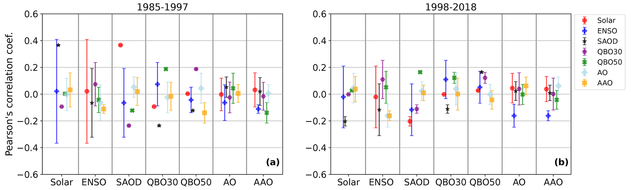
Figure 1 Pearson's linear correlation coefficients for different covariate variables (proxy variables) of the SOCOLv4 ensemble experiment for the (a) ozone depletion phase (1985–1997) and the (b) ozone recovery phase (1998–2018). Error bars represent the 2σ standard deviation of correlation coefficients between ensemble members.

The independence of regressors is a crucial point of such an analysis. To this end, we performed a correlation test for each proxy from the 6 ensemble members of the experiment and 2 periods of analysis. Figure 1 illustrates the results of proxies correlation analysis.

The correlation test indicates generally low mutual dependencies, except for the correlation between solar radio flux and SAOD for the ozone depletion phase. The correlation between solar fluxes and volcanic activity has been investigated before (Kuchar et al., 2017). It is related to strong volcanic eruptions like Pinatubo and El Chichón that affected the atmosphere during the 1985–1997 period, which happened to synchronize with the solar cycle. The remaining proxies show the average correlation coefficients between −0.2 and 0.2, which is considered to be a “weak” mutual dependency.

It is important to note that in this study, all DLM calculations using model data as well as ozone composite and reanalyzes were performed for the entire 1985–2018 period. The evolution of the predicted variable is characterized in DLM by the so-called “trend-term” or background level. In simple terms, it is the evolution of a variable filtered from the known part of its variability, induced by external forcings, which are represented in DLM by proxies. The state of the predicted variable for the one-step-ahead is predicted by the Kalman filter, and the Kalman smoother is used for the marginal probability distribution of the state. The Markov Chain Monte Carlo (MCMC) method (Alsing and Ball, 2019) is used to infer the posterior distributions of the background level. Then, 200 samples of the background level were drawn from the DLM states, which describe the posterior distribution uncertainty. It was done to determine the standard deviation of the background level between these samples used to calculate the statistical significance of the results. Afterwards, the ozone trends per decade are calculated separately for the phases of the ozone evolution (between 1985 and 1997 and between 1998 and 2018) from the mean background level by applying the conventional linear regression (αx+β). In linear regression, α means a slope term, and hence, a trend per decade at each grid point (latitudes × heights) is calculated as α × length of month-to-month time series $/$ number of decades. Finally, the statistical significance is determined for each ensemble member using the mean background level and its standard deviation between MCMC samples by the Student's t test. The ensemble mean trends of the SOCOLv4 experiment are calculated as an average of the trends from all individual ensemble members. The statistical significance for the ensemble mean trends is calculated using a standard deviation of trends between individual ensemble members. Trends in BASIC ozone composite and reanalysis datasets were calculated using the same methodology but applying observed proxy variables in DLM, the same as presented in Ball et al. (2018) as it was mentioned above.

4 Results

4.1 Simulated long-term trends in O₃, ClO_x, BrO_x, NO_x, HO_x, and temperature for the ozone depletion and recovery phases

The explanation of simulated ozone trends for different atmospheric layers cannot be properly done without demonstrating the trends in reactive species involved in the ozone destruction cycles. In addition, the temperature is accounted for, because it controls the rate of chemical reactions for the formation of radicals and is an indicator of ozone change, since ozone is a radiatively active gas. Decadal trends in ozone as well as radicals and temperature from the SOCOLv4 ensemble mean results in both the ozone depletion and ozone recovery phases are presented in Fig. 2.

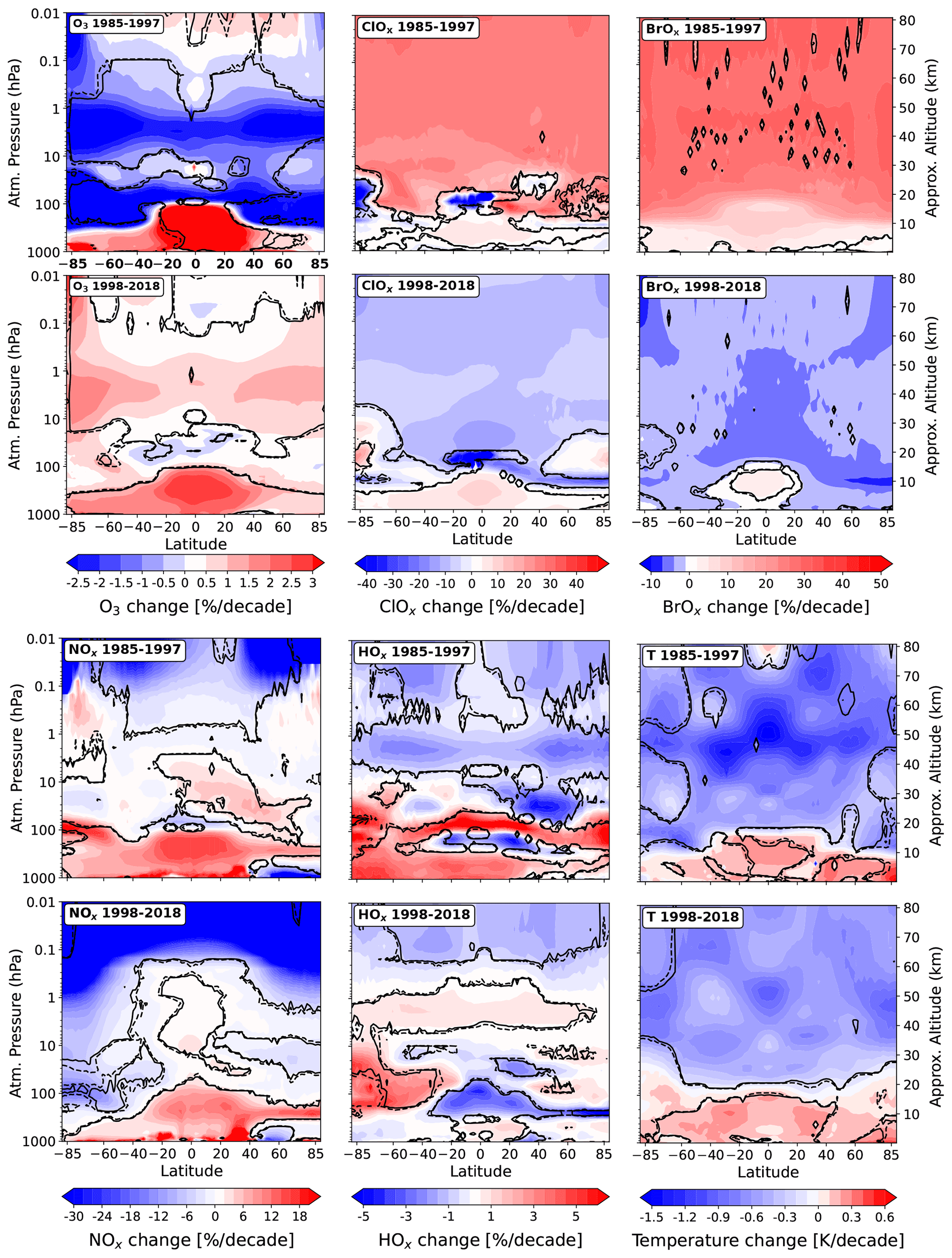
Figure 2 Ensemble mean trends of O₃, ClO_x, BrO_x, NO_x, HO_x (% per decade), and temperature (K per decade) from the SOCOLv4 results. The dashed line is the delimiter of the region with significance at the 90 % level for positive or negative changes; the solid line is the same at the 95 % level.

The radicals shown here are odd nitrogen [NO_x] = [NO] + [NO₂], odd hydrogen [HO_x] = [OH] + [HO₂], reactive chlorine [ClO_x] = [Cl] + [ClO], and reactive bromine [BrO_x] = [Br] + [BrO]. In the troposphere, an upward trend in NO_x is observed for both periods and it is stronger in the tropics. This positive trend is primarily due to the continuous increase in lightning activity and intensification of thunderstorms caused by global warming (Shindell et al., 2006) because the increase of the frequency of lightning flashes produces additional NO_x (Chameides et al., 1977; Sauvage et al., 2007). The NO_x due to aircraft emissions may also contribute to the positive trend in upper tropospheric NO_x (Köhler et al., 1997). Moreover, some tropospheric NO_x decrease related to the improved air quality is visible over the Northern Hemisphere. In addition, more intensive convective mixing can also intensify the upward transport of ozone precursors. In the mesosphere, NO_x strongly decreases in both periods. This is not related to solar activity; DLM excludes its contribution from evolution. It can be explained by the suppressed NO_x production due to the CO₂-related cooling in the mesosphere, which accelerates the cannibalistic NO + N → N₂ + O reaction. The same can be said about the negative trends in HO_x in the mesosphere, which are more pronounced and statistically significant in the region where the temperature decreases. In the upper stratosphere, HO_x trends follow ozone behavior because the HO_x production from water vapor strongly depends on the O(¹D) produced from the ozone. Furthermore, the decline in HO_x is observed in the upper tropical troposphere, which may be related to some dehydration processes (Ueyama et al., 2014). The simulated increase in ClO_x and BrO_x in the free tropical troposphere may be associated with an increase in emissions of very short-lived substances from the ocean and intensification of the atmospheric upwelling. In the middle atmosphere, both ClO_x and BrO_x show a statistically significant increase during the ozone depletion phase and a decrease during the ozone recovery phase. The temperature decreases in the middle atmosphere with a larger decline in the ozone depletion phase. In the troposphere, the temperature rises everywhere, with a stronger increase in the tropics and in the Northern Hemisphere.

4.2 Partial and total column ozone evolutions between 1985 and 2018

Figure 3 displays a comparison of the extra-polar (55^∘ N–55^∘ S), annual mean anomalies in partial and total column ozone (represented in Fig. 3 by the entire model atmosphere, upper right panel) for the 1985–2018 period simulated with SOCOLv4 and obtained from BASIC ozone composite as well as MERRA-2, ERA-5, and MSRv2 reanalyses.

Figure 3 Extra-polar (55^∘ N–55^∘ S), annual mean evolution of partial and total column ozone changes (in Dobson Units, DU) and DLM fits for the 1985–2018 period simulated with SOCOLv4 (red), from the Bayesian BASIC ozone composite (black), and from the reanalyses, including MERRA-2 (blue), ERA-5 (green), and MSRv2 (purple) for different atmospheric levels. Column ozone evolution and DLM fit presented for the (a) mesosphere; (b) upper stratosphere; (c) middle stratosphere; (d) lower stratosphere; (e) entire model atmosphere; (f) entire stratosphere, and (g) troposphere. The solid thin lines represent the ozone column anomalies; the solid curves represent the regression model fits computed by DLM, marked with the same color as the ozone anomalies. Red shadings represent 2σ standard deviation of ozone evolutions and DLM fits between ensemble members of SOCOLv4 results. Dashed-dotted vertical gray line marks the year 1998; dashed horizontal gray line marks the zero level.

It is worth noting that the mesospheric ozone evolution generally resembles the one in the stratosphere since the lower mesosphere in the model is still affected by the stratospheric ozone. In addition, mesospheric ozone does have a tiny positive contribution to the enhancement of the total column ozone (TOTOZ); it demonstrates a positive trend of ∼ 0.03 DU between 1998 and 2018.

The upper stratospheric ozone from both SOCOLv4 and BASIC demonstrates a pronounced decline during the ozone depletion phase, with a minimum after the Pinatubo eruption due to additional chlorine activation on volcanic aerosols. After 1998, the upper stratospheric ozone from both SOCOLv4 and BASIC began to increase distinctly. Yet, the upper stratospheric ozone evolution on the near-global scale in MERRA-2 and ERA-5 seems to be biased against BASIC and SOCOLv4 and does not reflect the evolution of hODS, with the hODS-induced ozone decline not appearing at all in MERRA-2 and being only scarcely presented in ERA-5. Meanwhile, ozone evolutions in the upper stratosphere during the recovery phase in MERRA-2 and ERA-5 are more reasonable but still hardly resemble those from BASIC and SOCOLv4.

In the middle stratosphere, SOCOLv4 shows a pronounced increase in ozone for a few years after the Pinatubo eruption due to an additional heterogeneous reactive uptake of N₂O₅ onto sulfuric acid particles, leading to a suppression of the NO_x catalytic ozone cycle (Prather, 1992; Solomon, 1999; Rozanov et al., 2002). BASIC does not show a similar increase in ozone, which might be because the effect of the Pinatubo eruption was filtered from the data due to some reported problems in satellite ozone retrieval during strong stratospheric aerosol loading (Davis et al., 2016; Ball et al., 2017). Unlike SOCOLv4, MERRA-2 and ERA-5 show a continuous decrease in middle stratospheric ozone until 1998 in MERRA-2 and around 2003 in ERA-5. In ERA-5, the start of ozone recovery due to the decrease in hODS is biased relative to BASIC and SOCOLv4 towards the beginning of the 2000s.

In the lower stratosphere, the ozone decline is seen in all presented datasets for the ozone depletion phase. The ozone minimum in this region has been visible for a few years after 1991 because of the enhancement of chlorine activation after the Pinatubo eruption (Solomon et al., 1993), after which ozone starts to recover. The LSO evolution in MERRA-2 shows a decline similar to SOCOLv4, while in ERA-5, the ozone decline is much stronger than in all other datasets. Starting from 1996, the LSO evolution is highly variable as a result of natural unforced variability. The extra-polar LSO evolutions from SOCOLv4 fluctuate around zero. BASIC shows the continuous decline of extra-polar LSO throughout the whole period, which is estimated to be 2 DU since 1998. In ERA-5 and MERRA-2, ozone evolution has completely opposite behavior during the last years of the period, showing either decline or increase, correspondingly. MERRA-2 and SOCOLv4 generally match each other and only a few years toward the end of the period, MERRA-2 shows a pronounced decline. ERA-5 demonstrates a much stronger increase in ozone during the ozone recovery phase, but the ozone starts to increase later than in other datasets and is virtually biased against BASIC and SOCOLv4.

Extra-polar tropospheric ozone in both SOCOLv4 and ERA-5 are similar, showing a pronounced increase throughout the whole period of ∼ 4 DU per period, which is facilitated by an increase in the number of ozone precursors, mainly NO_x (see Fig. 2) and CO. In the troposphere, MERRA-2 is not shown because it dramatically disagrees with expectations and other datasets. ERA-5 is more applicable in the troposphere, showing a general agreement with SOCOLv4.

Overall, the TOTOZ evolution modeled with SOCOLv4 is within the range of evolution from other datasets, for which the TOTOZ data are available. The TOTOZ evolution simulated with SOCOLv4 agrees better with MSRv2. For ERA-5, we see a much stronger increase in TOTOZ than in the other data presented, resulting from the abnormal ozone evolution in the stratosphere. MERRA-2 shows the marginal decline of TOTOZ compared to SOCOLv4 and other reanalyses, which may also be due to some flaws in these data, primarily for the stratosphere. Nevertheless, the presented time series display a general increase of the extra-polar TOTOZ. Yet, based on the obtained results, the important message is that the ERA-5 and MERRA-2 reanalyses still do not fit well for ozone trend analysis. We cannot demonstrate the source of this discrepancy, but it could be related to some issues with their underlying models, specific observational data processing, or assimilation approaches. We can be confident in saying that this is not related to DLM, as the evolution of ozone from these reanalyses prior to the application of DLM (dashed lines in Fig. 3) also exhibits this anomalous behavior. Yet, the MSRv2 reanalysis behavior is much smoother and more understandable, which agrees rather well with the SOCOLv4 simulations.

4.3 Simulated and observed long-term ozone trends for the ozone depletion and recovery phases

In this study, we first applied the regression model to the whole period (1985–2018), and then ozone changes for two phases of ozone evolution were computed from the DLM results. Figure 4 illustrates zonal mean decadal ozone trends between 1985 and 1997 in the ensemble mean SOCOLv4 reference experiment and from the BASIC observational composite.

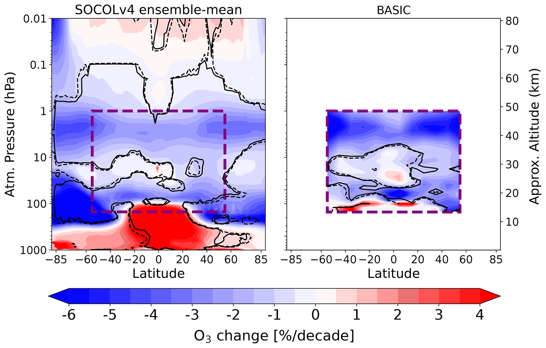
Figure 4 Ozone changes per decade (in %) for the ozone depletion phase (between 1985 and 1997) from the ensemble mean SOCOLv4 reference experiment and the BASIC observational composite. The dashed line is the delimiter of the region with significance at the 90 % level for positive or negative changes; the solid line is the same at the 95 % level. The dashed purple line indicates the region for which the BASIC composite is available.

For the ozone depletion phase, it is sufficient to show only the ensemble mean, since stratospheric ozone depletion due to hODS dominates any other effects on ozone evolution. The trend distribution calculated with SOCOLv4 is presented for the whole model atmosphere, i.e., from the ground to 0.01 hPa and for 90^∘ N–90^∘ S latitudes. For BASIC, the available region is only the extra-polar stratosphere (55^∘ N–55^∘ S). In the lower atmosphere, below the tropopause, it is seen that the model tropospheric ozone has a strong positive and statistically robust trend. The positive trend might result from continuous emissions of tropospheric ozone precursors; in the extra-polar region, it is mainly NO_x and CO (Griffiths et al., 2021). The chemical reactions that involve these precursors lead to ozone formation in the troposphere. We would like to emphasize that the positive trend of tropospheric ozone is getting stronger in the tropics (20^∘ N–20^∘ S), showing an increase of more than 4 % per decade that is attributed to increasing NO_x (see Fig. 2).

In high latitudes of both hemispheres, strong negative changes in ozone are observed in the lower stratosphere. Even if the Antarctic ozone hole is not a continuous event and occurs only during austral springtime, the pronounced and statistically significant negative changes of more than 6 % per decade are seen in the Southern Hemisphere, indicating the expansion of the ozone towards lower latitudes. The decline in ozone in the lower stratosphere of the Southern Hemisphere appears in SOCOLv4, even in the mid-latitudes (55–40^∘ S). As shown in Sukhodolov et al. (2021), the expansion of the ozone hole in SOCOLv4 is larger than in observations. It is related to overestimated isolation of the southern polar vortex area during wintertime (Sukhodolov et al., 2021). In the Northern Hemisphere, the negative lower stratospheric ozone changes also appeared. It should be noted that the strong ozone hole events over the Arctic are rather irregular, and usually, the Arctic ozone depletion is weaker than the one over the Antarctic (WMO, 2018). We obtained prominent, statistically significant negative ozone changes of about 4 %–5 % per decade over mid-to-high latitudes in the upper stratosphere of both hemispheres. This effect is observed because during this period, the continuous increase in halogen content strongly influenced the loss of ozone in these regions, and the catalytic ozone destruction cycle involving chlorine is more effective in the upper stratosphere due to the presence of a sufficient number of oxygen atoms (Chipperfield et al., 2018). Negative ozone trends from BASIC revealed in the upper stratosphere and over tropical lower stratosphere exceed those from SOCOLv4, showing depletion in ozone even more than 6 % per decade.

As it was mentioned above, the notable feature can be seen in the mesosphere, where SOCOLv4 demonstrates positive changes in ozone in the upper part of the mesosphere. This may be due to the NO_x and HO_x decline as was discussed above (see Fig. 2).

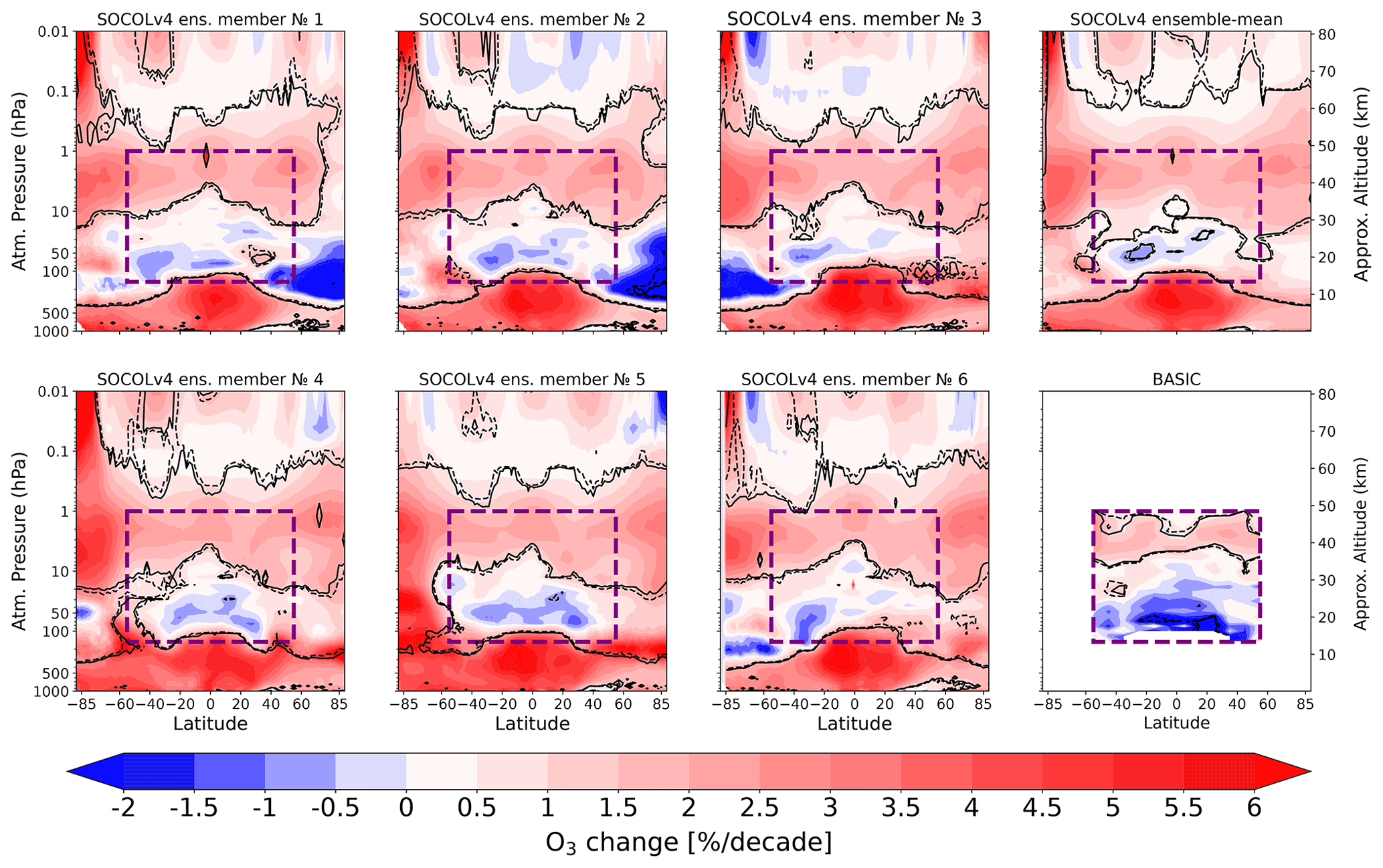
Figure 5 Zonal mean ozone changes for the ozone recovery phase (between 1998 and 2018) from the SOCOLv4 ensemble experiment and the BASIC observational composite (in percent per decade). The name of each ensemble member (or the ensemble mean) is indicated at the top of each panel. The dashed line indicates the region with significance at the 90 % level for positive or negative changes; the solid line is the same at the 95 % level. The dashed purple line indicates the region for which the BASIC composite is available.

The profile of decadal ozone trends between 1998 and 2018 from all individual ensemble members and ensemble mean of the SOCOLv4 reference experiment and BASIC observational composite are depicted in Fig. 5. For the recovery phase, we are particularly interested in analyzing and comparing the trend patterns from individual ensemble members to reveal how slightly different evolutions of the system, resulting in changes in natural unforced variability, affect the trend patterns.

For the ozone recovery phase, the tropospheric positive ozone changes with a similar magnitude remained stable, as the production of ozone precursors continued to increase for this period too (see Fig. 2). The tropical free-tropospheric ozone shows an increase of ∼ 4 %–5 % per decade. In the lower stratosphere, in defiance of recovery, the ozone in high latitudes of both hemispheres is not showing the increase in all presented ensemble members of the experiment and even demonstrates signs of negative changes. In three out of six ensemble members, there are regions with a manifestation of negative signal in ozone, either in the northern or southern high latitudes, which might be artifacts as they are not significant. This may be related to an underestimation of ozone production or abnormal dynamical perturbations in these ensemble members during the recovery phase. The modeled extra-polar LSO changes are controversial. Yet, some slightly negative trends of ∼ 1 %–1.5 % per decade are observed in all ensemble members. It should be stated that positive, statistically significant trends in the extratropical lower stratosphere are also not observed and the ozone trends in this region diverge significantly between ensemble members as a result of the natural unforced variability. Despite the statistical significance being less than 90 % for a major part of the lower stratosphere and the magnitude being lower, the simulated trend patterns in ensemble members 4 and 5 largely correspond to the trend distribution revealed in the observations.

The middle stratospheric ozone from both SOCOLv4 and BASIC demonstrates a near-zero state, showing some signs of positive and negative changes but in general, the trend is not so different from zero.

In the upper stratosphere, the ozone increase of about 3 %–4 % per decade in mid-to-high latitudes is visible, statistically robust, and observed in all presented realizations of the SOCOLv4 reference experiment and BASIC composite as expected because of hODS limitation by Montreal Protocol, mainly ClO_x as well as temperature decrease (see Fig. 2). The simulated ozone changes in the upper stratosphere are slightly overestimating the BASIC by ∼ 1 % and have a more pronounced tendency to increase in a poleward direction. Note that the simulated ozone trends in the upper stratosphere do not vary much between ensemble members, showing generally similar distributions and magnitudes of trends. The mesospheric ozone shows an upward trend with a higher significance over the mid-latitudes of the Southern Hemisphere in most realizations, where a pronounced decline in NO_x and HO_x is observed (see Fig. 2). We would like to reemphasize that the possible ozone increase in the mesosphere is worth considering, since it can slightly contribute to the TOTOZ increase and compensate for some ozone decline in lower atmospheric levels to some extent.

5 Discussion and summary

In this paper, we examine long-term ozone trends computed with the SOCOLv4 in an ensemble with six members of a reference experiment and compare these realizations to data from the BASIC ozone composite and from a number of available reanalyses. The evolution of long-term ozone changes is quantified using dynamic linear modeling. In general, the ozone trends integrated across atmospheric layers (i.e., troposphere; lower, middle, and upper stratosphere; mesosphere) are well captured by SOCOLv4, although there are also some discernible deviations from the available observations and reanalyses. The model shows a continuous ozone increase during the entire period in the troposphere and for the recovery phase in the mesosphere as well as the upper and middle stratosphere, which is important to consider because they contribute positively to the overall enhancement of the TOTOZ.

Although ozone trends in SOCOLv4 are well simulated in most atmospheric layers, our study infers that the modeled ozone trends in the extra-polar lower stratosphere show significant variability in these trends across ensemble members. Indeed, detecting clear and robust ozone trends outside the polar regions in model simulations is difficult because of the high dynamical variability perturbing the individual ensemble members (Stone et al., 2018). This justifies the analysis of each ensemble member separately to study extra-polar LSO variability, as we do in the present work. We show that the model cannot fully reproduce the observed trends in LSO from 1998 to 2018. It may just be that our particular ensemble members do not follow the same dynamical trajectory that happened in reality. Therefore, the use of ensemble mean is not going to help if what happened during 1998–2018 in Earth’s atmosphere history is a statistical outlier. A better way to proceed is to conduct a larger ensemble of simulations and identify those simulations which do look a lot like what happened in reality, even if there are relatively very few of them. Then, diagnose that subset for the underlying causes of the shown LSO trends, as was done by Smith et al. (2020). Our analysis of 6 individual realizations for the ozone recovery phase revealed that the LSO trend patterns in ensemble members 4 and 5 show a better resemblance with observations than other members of the ensemble, suggesting that the natural variability in simulations may coincide, by chance, with the dynamical storyline that we have in our reality, i.e., in observations. Increasing the number of ensemble members to 100 or 1000 will increase the probability to get this pattern in the model atmosphere, which would allow obtaining ozone trends even closer to the observed ones. Such complication comes from the fact that the considered period is rather short and therefore, such small, not properly resolved dynamical fluctuations cause a very strong influence on trends. We cannot perform 1000 simulations, due to obvious computational limitations; however, the obtained range of results for this region in our work and that of Stone et al. (2018) already allows us to state that internal variability is a strong player in this game and its specific combination can produce various “technically” statistically significant results.

Recently, Godin-Beekmann et al. (2022) provided updated trends of the stratospheric ozone vertical distribution based on the LOTUS regression model, which relies on merged satellite records tested against ground-based records (but not using DLM). They confirmed the large influence of short-term dynamical variability, preventing solid conclusions on ozone trends in the extratropical lower stratosphere. Even small changes in time-series duration (±1 year) can affect the trend patterns (Ball et al., 2019). However, adding 3 more years between the original version of LOTUS and the update still did not produce statistically significant trends in LSO for the ozone recovery phase. Possibly, the ozone recovery phase is not yet long enough to detect statistically significant LSO trends in the LOTUS regression analysis (Godin-Beekmann et al., 2022). The attribution of all necessary regressors and their quality/completeness is also important to increase the robustness of the trend. In addition, the BASIC observational composite might have some limitations based on the quality and accuracy of measurements included in it.

Another very recent paper by Bognar et al. (2022) describes a new merged ozone profile dataset, based on SAGE II, SAGE III/ISS, and updated OSIRIS data. Trends are determined by using and comparing MLR and DLM analyses. For the 2000–2021 period, they show that ozone decreased by 1 %–3 % in the lower stratosphere since 2000. These decreases were found to be more pronounced in DLM than in MLR, and significant in the tropics (> 95 % confidence), but not necessarily at mid-latitudes (> 80 % confidence). They further highlight that in tropopause relative coordinates, most of the negative trends in the tropics lose significance, highlighting the impacts of a warming tropopause and increasing tropopause altitudes. We should emphasize the need to find out what the ozone changes in the extra-polar lower stratosphere are related to.

They may be to a certain degree, induced by uncertainties in emissions, particularly on greenhouse gases, ozone-depleting substances, anthropogenic very short-lived substances (Barrera et al., 2020) including iodine-containing species (Karagodin-Doyennel et al., 2021), and volcanic aerosol loading. Other factors might concern structural uncertainties of the models, such as their horizontal and vertical resolution, in the upper troposphere and lower stratosphere as well as insufficient treatment of diffusion and transport processes (Dietmüller et al., 2017, 2018).

Regardless of the lower stratospheric ozone issues in the model, the modeled TOTOZ shows a continuous increase during the ozone recovery phase that is in good agreement with the MSRv2 reanalysis. Yet, we should stress that other reanalyses used in our study, such as the MERRA-2 and ERA-5, are less suitable for ozone trend analysis because they have artifacts from unknown origin that interfere with a correct trend estimate. It is beyond the scope of this study to explain the biases in the different reanalysis datasets. They could stem from some issues with their underlying models, from observational uncertainties, specific data retrievals, or be dependent on the assimilation technique.

In summary, the trends identified by SOCOLv4 are largely consistent with previous findings and confirm the general understanding of ozone recovery, including the effects of climate change on the ozone layer. The model results further confirm that there are marginally significant negative ozone changes in parts of the low-latitude lower stratosphere. This result generally agrees with the negative trends extracted from satellite data composite, however, the simulated magnitude and significance are lower than in observations. Thus, further efforts should be directed to carrying out model experiments with a higher number of ensemble members to address the higher part of the system uncertainty, which have to increase the chances to reproduce the observed pattern of atmospheric variability in the model. It is also necessary to continue work on reducing the uncertainty of the boundary conditions. Nevertheless, the presented results indicate a good level of agreement between the model and observations, allowing the production of reliable estimates of future ozone evolution using contemporary Earth system models.

Appendix A

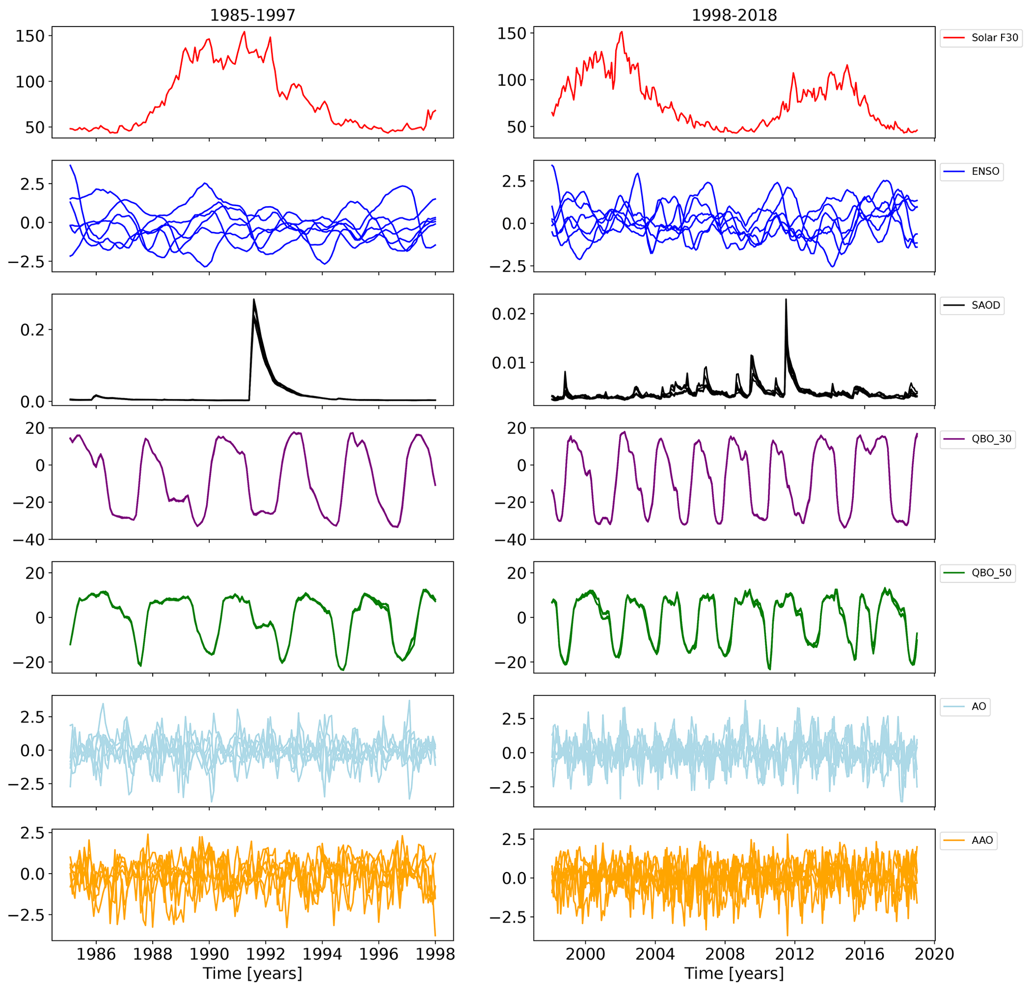
Figure A1 Input quantities (proxy variables) for the forcing of the SOCOLv4 ensemble experiment.

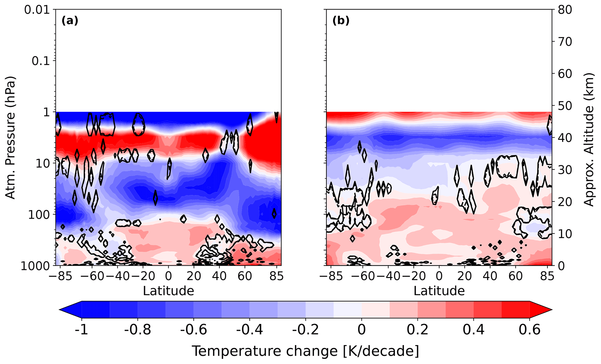
Figure A2 Profiles of temperature trends (K per decade) obtained from the ERA-5 reanalysis dataset. (a) Ozone depletion phase (1985–1997); (b) ozone recovery phase (1998–2018). The dashed line indicates the region with significance at the 90 % level for positive or negative changes, the solid line is the same at the 95 % level.