Cluster-based characterization of multi-dimensional tropospheric ozone variability in coastal regions: an analysis of lidar measurements and model results

Coastal regions are susceptible to multiple complex dynamic and chemical mechanisms and emission sources that lead to frequently observed large tropospheric ozone variations. These large ozone variations occur on a mesoscale and have proven to be arduous to simulate using chemical transport models (CTMs). We present a clustering analysis of multi-dimensional measurements from ozone lidar in conjunction with both an offline GEOS-Chem chemical-transport model (CTM) simulation and the online GEOS-Chem simulation GEOS-CF, to investigate the vertical and temporal variability of coastal ozone during three recent air quality campaigns: 2017 Ozone Water-Land Environmental Transition Study (OWLETS)-1, 2018 OWLETS-2, and 2018 Long Island Sound Tropospheric Ozone Study (LISTOS). We developed and tested a clustering method that resulted in five ozone profile curtain clusters. The established five clusters all varied significantly in ozone magnitude vertically and temporally, which allowed us to characterize the coastal ozone behavior. The lidar clusters provided a simplified way to evaluate the two CTMs for their performance of diverse coastal ozone cases. An overall evaluation of the models reveals good agreement (R≈0.70) in the low-level altitude range (0 to 2000 m), with a low and unsystematic bias for GEOS-Chem and a high systemic positive bias for GEOS-CF. The mid-level (2000–4000 m) performances show a high systematic negative bias for GEOS-Chem and an overall low unsystematic bias for GEOS-CF and a generally weak agreement to the lidar observations (R=0.12 and 0.22, respectively). Evaluating cluster-by-cluster model performance reveals additional model insight that is overlooked in the overall model performance. Utilizing the full vertical and diurnal ozone distribution information specific to lidar measurements, this work provides new insights on model proficiency in complex coastal regions.

1 Introduction

Tropospheric ozone (O₃) is an important secondary pollutant created by multiple reactions involving sunlight, nitrogen oxides (NO_x = NO + NO₂), and volatile organic compounds (VOCs), which, in accumulation, can have damaging effects on human and plant health. In addition to its photochemical growth, O₃ can easily be influenced by local and regional transport mechanisms. For coastal regions, surface O₃ is highly variable in time and space due to its susceptibility to many factors such as local ship emissions, long-range transport, and sea/bay breeze processes. This variability is challenging for air quality models to capture as high-resolution measurements are necessary to fully understand and simulate this O₃ behavior in coastal regions.

For example, Dreessen et al. (2019) tested the U.S. Environmental Protection Agency (EPA) Community Multiscale Air Quality (CMAQ) model's ability, configured at 12 km, to simulate O₃ exceedances at Hart Miller Island in Maryland (HMI) revealing high bias and “false alarms” due to several factors such as emission transport over water and the coarse model resolution's inability to capture fine-scale meteorology and transport. Multiple studies have proven the strong influence that sea/bay breeze and wind flow patterns can have on the accumulation of coastal O₃ and can often lead to poor air quality (e.g., Tucker et al., 2010; Martins et al., 2012; Stauffer et al., 2012; Li et al., 2020). Cases such as sea/bay breeze events, which directly contribute to high coastal O₃ cases, are denoted by local meteorological mechanisms such as surface wind speed deceleration, wind direction convergence, and recirculation (Banta et al., 2005). Loughner et al. (2014) also highlighted the importance of understanding the ability bay breeze events have in O₃ variability not only spatially but vertically throughout the atmosphere. Air quality models with coarse horizontal and vertical resolutions are not able to capture such fine developments (Caicedo et al., 2019). Ring et al. (2018) also used CMAQ to estimate the impact of ship emissions on the air quality in eastern US coastal regions indicating that an understanding of the vertical profiles of emissions was significant for improving air quality simulations. These are consistent and unanimous issues with air quality modeling in coastal regions. Since offshore sites within coastal regions are historically undersampled due to the difficulty of water-based measurements, this problem is still pertinent today.

Recently, three associated air quality campaigns have set out to address this issue (https://www-air.larc.nasa.gov/index.html, last access: 20 January 2021): the 2017 and 2018 NASA Ozone Water-Land Environmental Transition studies (OWLETS-1 and OWLETS-2) and the Long Island Sound Tropospheric Ozone Study (LISTOS) (e.g., Sullivan et al., 2019). These three campaigns were each conducted in highly populated coastal regions along the Chesapeake Bay in Virginia and Maryland and the Long Island Sound in the New England/Middle Atlantic region, which are vulnerable to O₃ exceedances, with the goal of filling the measurement gaps in these regions. During these campaigns, a suite of detailed airborne and ground measurements were taken during the course of highly polluted summer months (end of May through August) to capture the variability of pollutants, including O₃ and its precursor species, and the distinct meteorological processes specific to land–water regions that affect them.

The three campaigns strategically placed multi-dimensional tropospheric O₃ lidar instruments on and offshore in order to capture critical land–water gradients and to fill the deficit of measurements in these under-monitored areas. These measurements were supported as part of NASA's Tropospheric Ozone Lidar Network (TOLNet). Continuous profile measurements from O₃ lidars highlight important regional transport and temporal variations in O₃ in the lower and middle levels of the troposphere that are usually difficult to capture by most satellite-based remote-sensing instruments (Thompson et al., 2015). Lidar instruments are unique in their ability to capture high-resolution full O₃ 2-D profile curtains over a period of time that can help in understanding O₃ behavior in coastal regions. In Gronoff et al. (2019), the co-located lidar at the Chesapeake Bay Tunnel Bridge (CBBT) during OWLETS-1 successfully captured a near-surface maritime ship plume emission event on 1 August 2017. An ensemble of other instruments (e.g., drones, Pandora spectrometer systems) launched near the shipping channel captured elevated NO₂ concentrations, while the lidar instrument captured a depletion of O₃ simultaneously. The lidar was able to capture the unique low-range altitude O₃ concentrations which elucidated the evolution of the trace-gas concentrations during this ship plume event.

Several studies have thoroughly evaluated the results from the air quality campaigns used in this study but were focused more on specific case studies (Dacic et al., 2020; Sullivan et al., 2019; Gronoff et al., 2019). Dacic et al. (2020) used lidar measurements of a high-O₃ episode during OWLETS-1 to evaluate the ability of two NASA coupled chemistry–meteorology models (CCMMs) – the GEOS Composition Forecast (“GEOS-CF”; Keller et al., 2021) and MERRA2-GMI (Strode et al., 2019) – to simulate this high-O₃ event. They found that the GEOS-CF model performed fairly in simulating O₃ in the lower level (between 400 to 2000 $\mathrm{m}\mathrm{a}.\mathrm{s}.\mathrm{l}.$) and outperformed MERRA2-GMI based on surface observations at multiple monitoring sites. In the case of this event, GEOS-CF was able to simulate the 2-D O₃ profile curtains at small scales. At the time of the Dacic et al. (2020) study, processed observational data were only available from OWLETS-1.

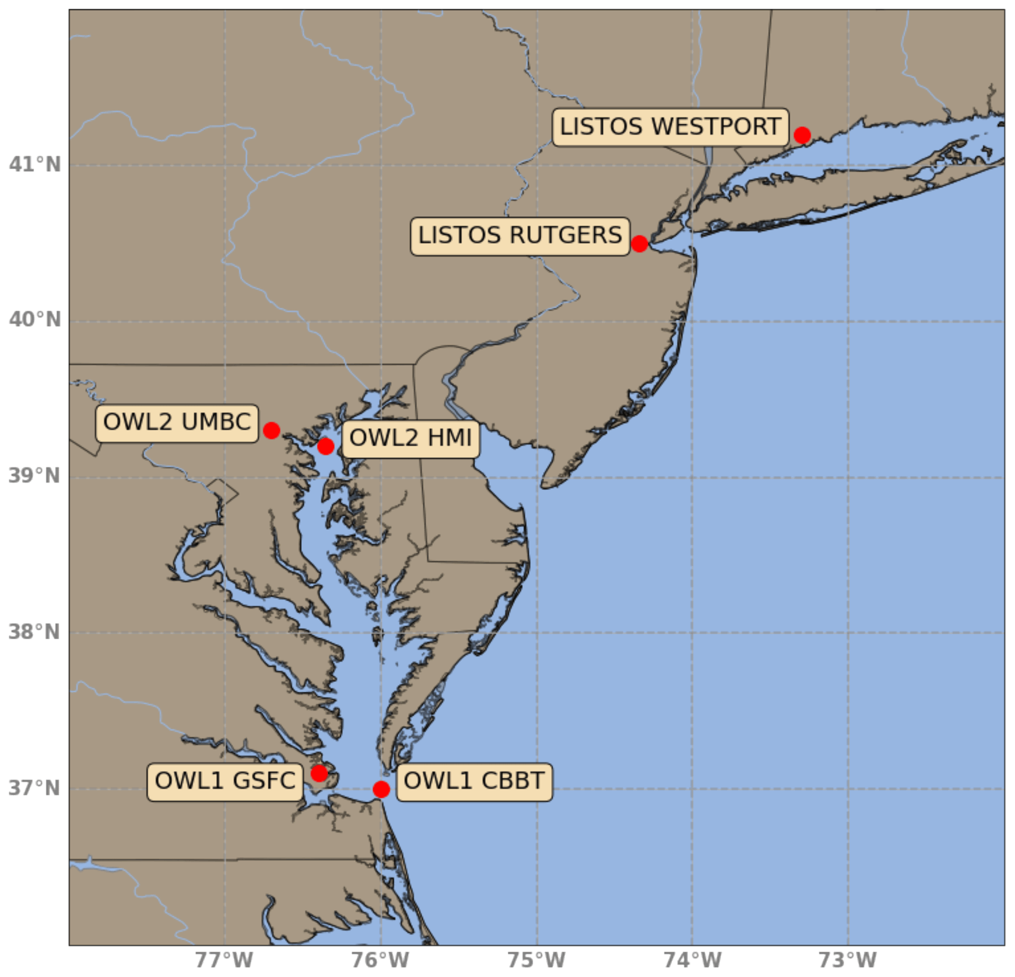
Figure 1 An inset map of the Chesapeake Bay airshed in Maryland, Virginia, and Long Island Sound in New York with the six lidar monitoring locations used for OWLETS-1, OWLETS-2, and LISTOS highlighted and labeled.

For this study, we took advantage of measured 2-D (vertical and diurnal) O₃ profile curtains from all three air quality campaigns (Sect. 2). To characterize the different behaviors of O₃ in coastal regions, we developed a novel clustering method based on the altitude and time dimensions of the lidar measurements that organized the profile curtains (Sect. 2). We used the developed clusters to evaluate the ability of both offline and online GEOS-Chem and GEOS-CF simulations to reproduce the coastal O₃ and wind characteristics highlighted by each cluster (Sect. 3).

2 Materials and method

2.1 Air quality campaigns

During the years 2017 and 2018, NASA in partnership with other US national agencies and university research groups orchestrated three air quality campaign studies that focused on key land and water observations: OWLETS-1, OWLETS-2, and LISTOS. OWLETS-1 was conducted in 2017 from 5 July to 3 August, while OWLETS-2 and LISTOS were conducted in 2018 from 6 June to 6 July and 12 July to 29 August, respectively. All campaigns took advantage of a multitude of ground, aircraft, and remote-sensing measurements. For the sake of this study, we will focus on measurements from the two lidars from the TOLNet: the NASA Langley Mobile Ozone Lidar (LMOL) (De Young et al., 2017; Farris et al., 2019; Gronoff et al., 2019, 2021) and NASA Goddard Space Flight Center (GSFC) Tropospheric Ozone (TROPOZ) Differential Absorption Lidar (DIAL) (Sullivan et al., 2014, 2015a), which ran simultaneously at the marked positions in Fig. 1. The TOLNet data from all three campaigns are available on the NASA Langley Research Center (LaRC) Airborne Science Data for Atmospheric Composition archive (https://www-air.larc.nasa.gov/missions.htm, last access: 20 January 2021).

The two lidars were placed strategically for each campaign (Fig. 1), so that one lidar was closest to over-water measurements, while the other was farther inland with the goal of examining how O₃ transport and concentration are influenced by specific coastal mechanisms such as the land–water breezes. For OWLETS-1, the LMOL lidar was used at the CBBT (37.0366^∘ N, 76.0767^∘ W), depicting the real time over-water O₃ measurements, while the GSFC TROPOZ lidar was stationed at the NASA Langley Center (37.1024^∘ N, 76.3929^∘ W) further inland. Similarly, for OWLETS-2, the LMOL lidar was stationed for the over-water measurements at Hart Miller Island (39.2449^∘ N, 76.3583^∘ W) and GSFC TROPOZ was stationed at the University of Maryland, Baltimore County (UMBC) (39.2557^∘ N, 76.7111^∘ W). For LISTOS, LMOL was at the Westport site (41.1415^∘ N, 73.3579^∘ W) and TROPOZ at Rutgers (40.2823^∘ N, 74.2525^∘ W). For the sake of this study the unique benefits due to the different placements (onshore versus offshore) of the co-located lidars are not specifically evaluated. Instead, the study focuses on the benefits of the detail and multi-dimensionality of lidar instrument data in general.

Routine lidar measurements were taken for the duration of the campaigns. Both lidars retrieve data at a 5 min temporal resolution and use a common processing scheme to produce a final O₃ product which was used for this study. In this study, the individual profile curtains refer to the “full-day”, vertical and diurnal lidar measurements. In this study, 91 individual 2-D profile curtains were used from both lidars from the three campaigns: 26 profile curtains from OWLETS-1, 28 profile curtains from OWLETS-2, and 37 profile curtains from LISTOS.

To evaluate meteorological impacts on the lidar O₃ clusters and model performance, we used various temperature and wind measurements. Hourly observed temperature, wind speed, and wind direction and O₃ from surface monitors pertaining to the study area were obtained from the Air Quality System (AQS) (data can be accessed at https://aqs.epa.gov/aqsweb/airdata/download_files.html, last access: 17 December 2020). We utilized high-resolution vertical and horizontal wind speed and direction data monitored by Doppler wind lidar Leosphere WINDCUBE 200s instruments deployed at HMI during OWLETS-2 and during LISTOS (e.g., Couillard et al., 2021; Coggon et al., 2021; Wu et al., 2021).

2.2 Clustering lidar data

2.2.1 Description of the ozone lidar measurements

The lidar instrument is unique in that it provides high-dimensional profile measurements of O₃, as opposed to one-dimensional surface measurements from air quality monitoring sites. The two TOLNet lidars used during the campaigns have been evaluated for their accuracy during previous air quality campaigns (DISCOVER-AQ, https://www-air.larc.nasa.gov/missions/discover-aq, last access: 29 November 2022 and FRAPPÉ, https://www2.acom.ucar.edu/frappe, last access: 29 November 2022) and have also been compared against each other (e.g., Sullivan et al., 2015b; Wang et al., 2017). The two lidars have different transmitter and retrieval components but produce O₃ profiles within 10 % of each other as well as compared to ozonesondes (Sullivan et al., 2015b). In comparison with other in situ instrument measurements, the TOLNet lidars were found to have an accuracy better than ± 15 % for capturing high temporal tropospheric O₃ vertically proving their capability of capturing high temporal tropospheric O₃ variability (Wang et al., 2017; Leblanc et al., 2018).

To characterize coastal O₃ during the summer months, we use a multitude of lidar profile curtains obtained during the OWLETS-1 and 2 and LISTOS campaigns. The two lidars used in the campaigns produced O₃ profile curtains from 0–6000 m above ground level ($\mathrm{a}.\mathrm{g}.\mathrm{l}.$) with some days beginning as early as 06:00 LT (EDT) and ending measurements as late as the last hour of the day. One of the challenges is that the multiple lidar datasets are not always uniform; although most of the profile curtains began at or around 08:00 EDT, the lidar measurements commence and conclude at different times. At the time of these campaigns, the lidar data retrieval was constrained by the availability of personnel as well as the availability of electricity in remote areas. Due to this constraint, the 91 lidar curtains range from as short as a 6 h window to a full 24 h window. Similarly, the profile curtains do not have an exact uniform altitude range either. In the processing of the lidar data, some measurements may be filtered out and removed due to issues, such as clouds, which can influence and degrade the retrieval leaving some blocks of empty data within the vertical altitude dimension. When the cloud conditions are perfect, the limiting factor for the altitude is the solar background: the UV from the sun is a source of noise that prevents the detection of the low level of backscattered photons. For LMOL, this means that the maximum altitude is about 10 $\mathrm{km}\mathrm{a}.\mathrm{g}.\mathrm{l}.$ at night (Gronoff et al., 2021) and lowered to about 4 $\mathrm{km}\mathrm{a}.\mathrm{g}.\mathrm{l}.$ at solar noon (worse conditions possible for the summer in the continental US resulting in below 4 $\mathrm{km}\mathrm{a}.\mathrm{g}.\mathrm{l}.$). This results in a general scarcity of O₃ measurements above 4000 $\mathrm{m}\mathrm{a}.\mathrm{g}.\mathrm{l}.$ for most of the vertical profile curtains. Lidars still have limitations that prove to be a complication, e.g., noise signal and manual operations. At the time of writing, the operative limitation has been addressed and the lidars are now more fully automatized for use during succeeding campaigns, removing such constraints.

2.2.2 Clustering approach and application

To characterize coastal O₃, we used a cluster analysis to categorize the behavior of the tropospheric O₃ captured in the profile curtains. Clustering methods are commonly used in air quality and atmospheric studies to group and characterize large datasets (Darby, 2005; Alonso et al., 2006; Christiansen, 2007; Davis et al., 2010; Stauffer et al., 2018). In our previous work, we have successfully used clustering methods to automatically characterize diurnal patterns of surface winds and surface O₃ in the Houston–Galveston–Brazoria area that proved to perform better than a rudimentary quantile method to reveal the dependence of surface O₃ variability on local and synoptic circulation patterns on the Gulf Coast (Bernier et al., 2019; Li et al., 2020).

In evaluating the structure of the lidar measurements and working within measurement limitations (described in Sect. 2.2.1) from the three air quality campaigns, we developed a method to cluster multi-dimensional O₃ profile curtains using K-means clustering algorithm. Input features (seed values) were rationally established to best represent the behavior of O₃ temporally and vertically without including an excessive number of input features, which can weaken the results of clustering (discussed in detail in Sect. S1 in the Supplement). With the goal of evaluating lower-level tropospheric O₃ and based on description of the structure and constraints of the lidar measurements, the features were tailored to the altitude range of 0–4000 $\mathrm{m}\mathrm{a}.\mathrm{g}.\mathrm{l}.$ and time range of 06:00–21:00 EDT.

Figure 2 illustrates the eight features that represent the slabs of altitude and time used in the cluster analysis. For each O₃ profile curtain (total of 91), we calculated the average O₃ from the following time and altitude range: Feature 1–4 altitudes range from 0–2000 m; Feature 5–8 altitudes range from 2000–4000 m. The two altitude ranges were determined to best represent different O₃ transport events, although they do not explicitly represent these layers. For Features 1–4, O₃ would most likely primarily be affected by local production and pollution transport, while for Features 5–8, O₃ would more likely be associated with long-range transport (e.g., interstate). As planetary boundary layer growth (PBL) in coastal regions does not usually reach altitudes greater than 2000 m, mixing between the boundary layer and free troposphere would presumably take place within the low-level altitude bin. Additional attention to the PBL in the selecting of low versus mid-level features for the clustering will be investigated in future work. For clarity, we will use the terms low-level and mid-level features to address the two altitude subsets, e.g., Features 1–4 and 5–8, respectively. Feature 1 and 5 times range from 06:00–08:00 EDT; those of Feature 2 and 6 from 08:00–12:00 EDT; those of Feature 3 and 7 from 12:00–16:00 EDT; and those of Feature 4 and 8 from 16:00–21:00 EDT. The four subset time ranges were indicated to best represent features that characterize the common diurnal behavior of O₃.

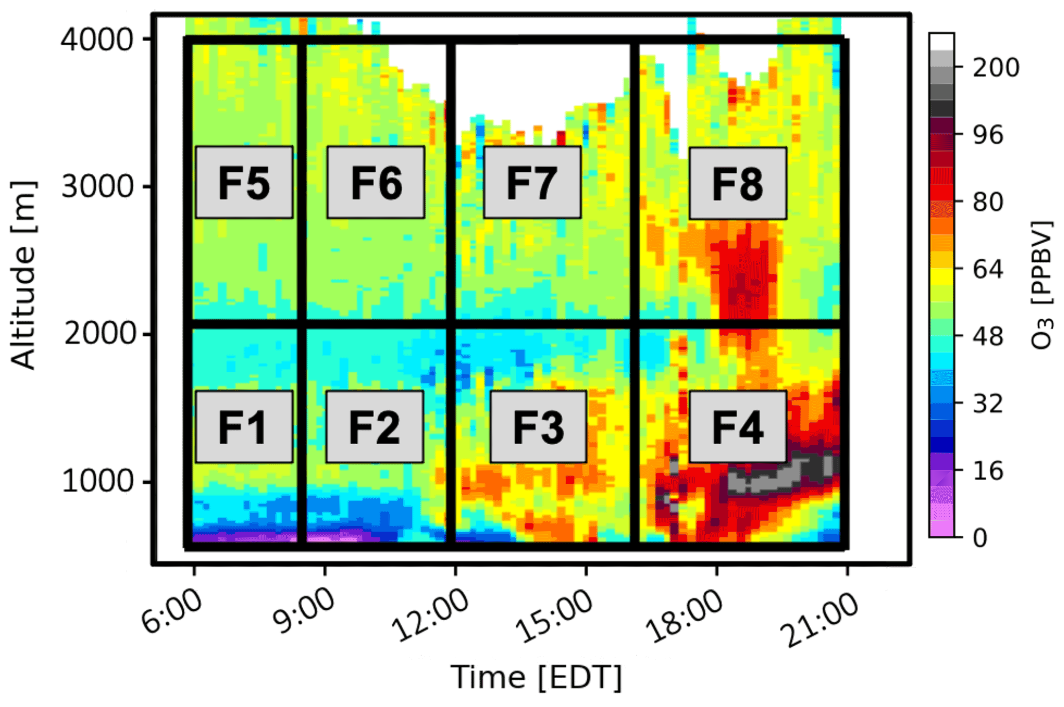
Figure 2 The clustering method developed for clustering vertical O₃ profiles taken from lidar measurements. The color coding shows a typical day of lidar measurements of O₃ profiles on 6 August 2018, from the LMOL at Westport, CT, during the LISTOS Campaign. F1–F8 indicate the time and altitude range of the eight features used for the clustering algorithm.

The features were evaluated for cluster tendency, essentially to confirm our dataset contained meaningful clusters (discussed in detail in Sect. S2 in the Supplement). Evaluating different feature options did not lead to better statistical results than with the final chosen features. Since the choice of clustering algorithm is subjective, we chose K-means clustering for its simplicity and widespread use. To use the K-means clustering algorithm, the optimal number of clusters based on your dataset must be chosen beforehand (Sect. S2). We selected six clusters as the optimal number of clusters. Since the K-means clustering algorithm is based on the Euclidean distance to each centroid, the input data were normalized (to a mean of 0 and standard deviation of 1) to ensure each feature is given the same importance in the clustering (Aksoy and Haralick, 2001; Larose, 2005).

The clustering analysis initially identified six clusters (described fully in Sect. 3.2). Only one date was assigned to Cluster 6 (16 June 2018): the lidar profile curtain on this day (Fig. S1 in the Supplement) shows a large fraction of data missing, and the available data have relatively high O₃ throughout the lowest 3 km, which is different from other clusters. Therefore, we consider Cluster 6 to be an outlier and will not be included in the subsequent analysis.

2.2.3 Missing data

Although the input features were tailored based on the structure of the lidar measurements, the remaining data still had missing data points. In performing a quick evaluation on the eight input features (Fig. S6 in the Supplement), we found that Features 1, 4, 5, and 8 had the most missing data, while Features 2, 3, 6, and 7 had few or zero cases of missing data. This means that the earlier morning measurements (06:00–12:00 EDT) and the later evening measurements (16:00–21:00 EDT) had the most cases of missing data points. This is plausible as the campaign teams were best able to retrieve clear measurement during midday/evening hours (12:00–16:00 EDT). As a result, 51 out of 91 O₃ profile curtains had at least one missing data point (feature) throughout the individual profile curtain.

A common practice for dealing with missing data is complete case analysis (CCA), in which observations with missing values are completely ignored, leaving only the complete data to cluster. CCA can be inefficient as it introduces selection bias since the sample data no longer retain the state of the original full dataset (Donders et al., 2006; Little and Rubin, 2014). When we applied CCA, there were only 40 O₃ profile curtains of complete data, removing over half of the study profiles. Instead, we used a more comprehensive solution – imputation – that yields results (Donders et al., 2006). For this study we used the single imputation (SI) technique, knnImputation, which uses the k-nearest neighbors and searches for the most similar cases and uses the weighted average of the values of those neighbors to fill in the missing data (Torgo, 2011). Essentially, this method selects the days that have the most similar profile curtain to any profile which has missing data points and uses those real data points to calculate a weighted mean that will fill in the missing data. We acknowledge using an imputation method on the dataset will possibly introduce a bias which is difficult to quantify, but this allows us to utilize all 91 O₃ profile curtains. The silhouette method was used to test the quality of the newly imputed dataset, which proved to be neither worse nor better than the CCA (real data) results. Therefore, the dataset was first imputed using SI to create a complete dataset, and then the clustering method described in the section before (Sect. 2.2.2) was applied to the complete imputed dataset.

2.3 Model simulations

The offline GEOS-Chem chemical-transport model (CTM) was utilized to simulate the spatial and temporal variability of coastal O₃ in the Chesapeake Bay and Long Island Sound during the time of the campaigns. The GEOS-Chem model is a global 3-D CTM driven by assimilated meteorological data from the NASA Global Modeling and Assimilation Office (GMAO). Our simulations were driven by reanalysis data from Modern-Era Retrospective analysis for Research and Applications, Version 2 (MERRA-2; Gelaro et al., 2017). We ran a nested GEOS-Chem (v12-09) simulation at 0.5^∘ × 0.625^∘ horizontal resolution over the eastern portion of North America and the adjacent ocean (20–50^∘ N, 90–60^∘ W), using lateral boundary conditions updated every 3 h from a global simulation with 2^∘ × 2.5^∘ horizontal resolution. The nested GEOS-Chem simulation was run with 72 vertical levels from 1013 to 0.01 hPa. Since the study focuses on the altitude range of 0–4000 m, the first 20 vertical levels from GEOS-Chem were used with 14 levels within the boundary layer (≤ 2000 m). The nested simulation was conducted for the study periods June–September 2017 and April–August 2018. We used the standard “out-of-the-box” unmodified default settings from the tropospheric chemistry chemical mechanism (tropchem) with global anthropogenic emissions from the Community Emissions Data System (CEDS) inventory (McDuffie et al., 2020) and the U.S. Environmental Protection Agency (EPA) National Emissions Inventory (NEI) 2011 for monthly mean North American regional emissions (EPA NEI, 2015).

We also used results from NASA's near real-time forecasting system, GEOS-CF, an online GEOS-Chem simulation (v12-0-1) from GMAO (https://gmao.gsfc.nasa.gov/-weather_prediction/GEOS-CF/ last access: 2 February 2022) with GEOS coupled to the GEOS-Chem tropospheric–stratospheric unified chemistry extension (UCX) and run at a high spatial resolution of 0.25^∘, roughly 25 km (Keller et al., 2021; Knowland et al., 2021). The vertical resolution for GEOS-CF is interpolated onto 72 vertical levels from 1000 to 10 hPa. Since the study focuses on the altitude range of 0–4000 m, the first 21 vertical levels from GEOS-CF were used with 14 levels within the boundary layer (≤ 2000 m). Prior to the launch of the 12Z 5 d forecast, GEOS-CF produces daily global, 3-D atmospheric composition distributions using the GEOS meteorological replay technique (Orbe et al., 2017), and this study makes use of these historical estimates, made available to the public for the period since January 2018. Therefore, the GEOS-CF results shown in this study only include the dates from the OWLETS-2 and LISTOS campaigns, since they both occurred in 2018.

While both model simulations use similar versions of GEOS-Chem chemistry, there are noteworthy differences to keep in mind during the analysis of the clustering. The main differences between the two models are (1) GEOS-Chem is an offline CTM using archived meteorology, while GEOS-CF simulates atmospheric composition simultaneously with meteorology (online); (2) the spatial resolution of the GEOS-CF model (0.25^∘) is higher than GEOS-Chem (0.5^∘ × 0.625^∘); and (3) the GEOS-CF model runs with Harmonized Gridded Air Pollution (HTAP; v2.2; base year 2010) anthropogenic emissions from the Emission Database for Global Atmospheric Research (EDGAR), while GEOS-Chem was run with CEDS anthropogenic emissions (base year 2014). These imperative differences can lead to disparities in the following results.

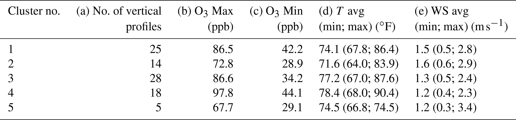
Table 1 Lidar vertical O₃ profile cluster statistics: (a) total number of vertical profiles; (b) O₃ maximum; (c) O₃ minimum. AQS monitoring station cluster mean (d) surface temperature and (e) wind speed (WS); minimum and maximums in parentheses. The statistics and averages were derived from the total number of profile curtains assigned to each cluster.

3 Results and discussion

3.1 Overview of the 2-D O₃ curtain clusters

The clustering results reveal distinctive characterized O₃ behavior during the three campaigns in which O₃ concentrations vary. Various O₃ and surface meteorological parameter cluster statistics for the five clusters are summarized in Table 1. With only five of the 2-D profile curtains assigned, Cluster 5 depicts the least common O₃ behavior during the campaigns. On the other hand, Cluster 3 is the most common O₃ behavior during the campaigns with 28 profile curtains assigned to this cluster. Following Cluster 3, Cluster 1 is the next most common cluster with 25 profile curtains. Cluster 2 and Cluster 4 fall in the middle with 14 and 18 profile curtains assigned to the cluster numbers, respectively.

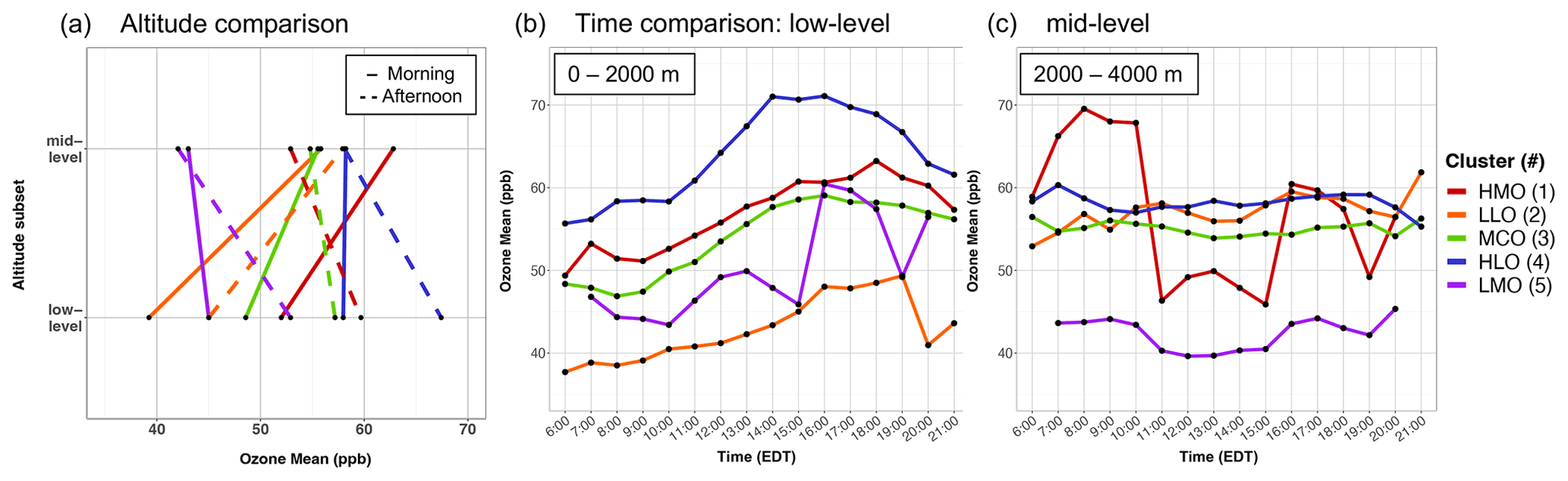
Figure 3 Lidar O₃ cluster average comparisons (five clusters depicted in colors). (a) Altitude comparison of mean O₃ averaged over time: morning hours from 6:00–12:00 (solid line) and afternoon hours from 12:00–21:00 (dashed lines). Time comparison of mean hourly O₃ split between the (b) low level and (c) mid-level.

The five clusters were distinguished by the varying O₃ concentrations between the low level and mid-level as well as diurnal variations (Fig. 3). In Fig. 3a we separate the data by the two altitude subsets (low and mid-level) and by morning (06:00–12:00) and afternoon (12:00–21:00) to quantify the between-cluster differences. In the low level, all five clusters exhibit the common O₃ diurnal pattern where surface O₃ is titrated overnight and reaches a minimum but then is quickly exacerbated with the increase in sunlight throughout the day and typically peaks after midday (Fig. 3b). The extent of this common diurnal pattern varies by cluster.

Cluster 1 in the low level has the second highest morning and afternoon O₃ average (52 and 59 ppb) and in the mid-level the highest morning O₃ average (64 ppb) (Fig. 3a). Cluster 1 also exhibits the most unique pattern of mid-level O₃ (Fig. 3c), with the highest concentrations found in the early morning and an uncharacteristic plunge to lower O₃ concentrations from 11:00–15:00 EDT. This is contrary to the other clusters which do not show much O₃ variation temporally in the mid-level. The majority of the individual profile curtains assigned to Cluster 1 show concentrated early morning residual layers in the mid-level that diffuse after the morning, which is distinctive compared to the other clusters. In the low level, Cluster 2 has the lowest morning and afternoon O₃ average among the clusters (39 and 45 ppb) with moderate mid-level O₃ concentrations. Cluster 3 has the most uniform vertical O₃ extent between the low and mid-level (Fig. 3a), in contrast to the other clusters that differ greatly in O₃ concentrations between the two altitude subsets. Cluster 4 has the highest morning and afternoon O₃ averages (59 and 68 ppb) in the low level, reaching > 70 ppb temporally (Fig. 3b). Finally, Cluster 5 has the considerably lowest morning and afternoon O₃ averages (42 and 43 ppb) in the mid-level, almost 10 ppb lower than the other clusters. Cluster 5 does not have a smoothly evolving O₃ diurnal pattern in the lower level (Fig. 3b), which can be attributed to the averaging of only five different profile curtains that were assigned to this cluster (Table 1).

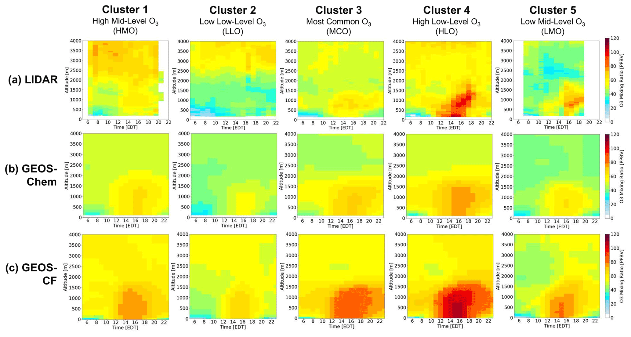
Figure 4 Cluster mean O₃ vertical profile results by cluster assignment (1–5) and arranged as follows: (a) lidar; (b) GEOS-Chem simulation; and (c) GEOS-CF simulation.

Figure 4a illustrates the mean lidar O₃ 2-D profile curtains for each of the clusters. For Clusters 1, 3, 4, and 5, higher O₃ concentrations in the low level are captured during afternoon/evening time (12:00–21:00 EDT), with the highest low-level O₃ in Cluster 4 (> 70 ppb). This behavior follows the common diurnal pattern of O₃ that was distinguishable in Fig. 3b. This common O₃ growth reaches vertically to approximately 1500 m for each of the clusters but is generally contained below 2000 m. Differing from the low-level O₃ behavior, mid-level O₃ is generally less variable in magnitude throughout the entire profile curtain (except for Cluster 1; see Fig. 3a). The highest O₃ concentrations for the mid-level are exhibited in Clusters 1, 2, 3, and 4, with the highest mid-level O₃ in Cluster 1 during the early morning hours (≥ 70 ppb).

Following the descriptions above, each cluster is given a nomenclature according to its unique characteristics: Cluster 1 is termed the highest mid-level O₃ (HMO) cluster; Cluster 2 is the lowest low-level O₃ (LLO) cluster; Cluster 3 is the most common O₃ (MCO) cluster; Cluster 4 is the highest low-level O₃ (HLO); Cluster 5 is the least common and lowest mid-level O₃ (LMO) cluster. The O₃ variability represented and justified above is what led to the successful clustering of the lidar O₃ 2-D profile curtains.

Figure 3b and c indicate that each cluster represents a different O₃ evolution pattern, likely related to different photochemical or transport regimes. This kind of evaluation is useful in that it combines O₃ information from both temporal and vertical dimensions. For example, the HLO cluster reveals a unique low-level case in which high O₃ concentrations at a high elevation (∼ 1000 m) are captured early in the temporal profile that translate to the higher O₃ concentrations at the surface later in the evening. The mean profile curtain indicates these cases did not have “clean air” to begin with which can allow a greater accumulation in the low level in the afternoon. In another example, several profile curtains assigned to the HMO cluster indicate concentrated residual layers in the mid-level and possible entrainment to the surface as the day progressed. To prove this feature, vertical velocity and vertical velocity variance data would be needed, but the knowledge that a clustering approach is able to highlight these features that could only be discernible through lidar measurements proves to be useful. The clustering results were valuable in recognizing a significant large pollution-related cluster (HLO), a total of 18 out of the 91 curtain profiles which correspond with the highest daily surface maxima measured at these sites (= 97.8 ppb) (Table 1). This cluster, on average, exhibited a daily surface maximum up to 10 ppb greater than any of the other clusters. Discerning these higher-O₃ cases is imperative for mitigating severe air pollution.

Figure 5 Cluster-averaged meteorological surface AQS station observations and GEOS-Chem model results. (a) Surface temperature observations represented as the circular markers and simulated surface temperatures represented as the spatial contour (top row). (b) Surface wind speed and direction observations represented as circular markers and white arrows and simulated wind speed and direction represented as spatial contour and black arrows (bottom row).

3.2 Cluster surface analysis

To support the lidar clustering results, daily averaged meteorological surface observations from AQS stations nearest to the lidar locations pertaining to the campaign period and GEOS-Chem surface model output were evaluated with regard to the five clusters. Figure 5 shows the cluster mean surface temperature from AQS stations and the GEOS-Chem model as well as the simulated wind speed and direction. The average surface temperature from each station is represented as the circular markers, while the simulated temperatures are represented as the spatial contour and the simulated wind speed (m s⁻¹) and direction as arrows. Cluster average and minimum and maximum AQS surface temperature and wind speed can be found in Table 1d and e.

In general, the surface meteorological conditions agree with our knowledge of transport and O₃ production that would lead to each of the five clustered lidar O₃ profile curtains. It is evident that the clusters with the highest surface O₃ (HMO, MCO, and HLO) all share a predominant offshore, westerly wind. Furthermore, MCO and HLO presented higher overall observed and simulated surface temperatures compared to the other clusters (Fig. 5a). These meteorological conditions are conducive to a higher production of surface O₃ concentrations which validates the higher O₃ found in the low-level results (Figs. 3b and 4a).

Conversely, the lowest surface temperatures are found in LLO. Lower surface temperatures are also indicative of low vertical mixing due to less generation of convection which can reduce any possible descending O₃ from aloft. Relatively calm wind speeds, lower temperatures, and other possible meteorological factors such as high cloud cover could have contributed to the lower O₃ concentrations in LLO. Although surface O₃ concentrations in LMO reach higher levels later in the day, first at 13:00 EDT and then again at 16:00 EDT, the rest of the temporal profile stays below moderate levels. Average temperatures for LMO are moderately high but, in contrast, the average wind speed is higher (specifically over the Long Island Sound) and unique to the other clusters, wind direction is predominantly onshore (easterly–southerly). This prevalent onshore flow indicates a transport of cleaner marine air which corroborates the lower surface O₃ levels. LMO did not have any profile curtains assigned from OWLETS-1, which is why data for the lower Chesapeake Bay area are not shown in Fig. 5.

There was only one occurrence during the dates in which the lidar instruments were operating in which there was a recorded maximum daily 8 h average (MDA8) O₃ exceedance (> 70 ppbv). This exceedance date is 25 May 2018, on which three AQS sites in the LISTOS region measured MDA8 O₃ of 73, 72, and 72 ppbv. This curtain profile was assigned to the HMO cluster (Cluster 1), the cluster with high O₃ in the mid-level and moderate O₃ in the low level and near the surface. Since the AQS stations applied here were the nearest stations to the lidar instrument placements, the MDA8 O₃ values captured by the AQS stations do not necessarily reflect the high O₃ concentrations captured by the lidars near the surface.

3.3 Evaluating the GEOS-Chem and GEOS-CF model

In this section the model results from GEOS-Chem and GEOS-CF will be compared to the lidar data using the five lidar O₃ profile clusters discussed in Sect. 3.1. Both model results were sampled in an equal manner, in which we extracted the same cluster date assignments from the lidar clusters and created mean vertical profiles based on the model results. This allowed us to evaluate the model performance based on the five characterized O₃ lidar clusters. As mentioned previously, the GEOS-CF simulation data are not available for 2017. Thus, the results shown subsequently will only include GEOS-CF results from 2018 (only dates from the OWLETS-2 and LISTOS campaigns). The GEOS-Chem simulation results include both years and thus all three campaign duration periods.

3.3.1 Overall model performance

Figure 4b and 4c depict the simulated cluster mean O₃ profile curtains from GEOS-Chem and GEOS-CF, mirroring the mean lidar profile curtains in Fig. 4a. For all clusters in the low level, both models simulate a consistent accumulation of O₃ near the surface after 12:00 EDT, mirroring the O₃ common diurnal pattern depicted in mean lidar profile curtains in Fig. 4a. However, the extent the models simulate is often higher in magnitude than the observations, specifically GEOS-CF consistently predicting the accumulation at a higher magnitude than GEOS-Chem. In the mid-level, both models simulate much less O₃ variability than what is captured in the lidar observations. Figure 4b and c clearly show how the models struggle to reproduce any mid-level O₃ pattern or variability that is relayed in the lidar observations.

We first evaluate overall correlation and biases between the model and lidar data, disregarding the specific clusters. The overall correlation between the models and the lidar data is evaluated by the two altitude subsets as the performances differ considerably between low level and mid-level for both GEOS-Chem (Fig. S7a in the Supplement) and GEOS-CF (Fig. S7b) (mean normalized biases found in Table S1 in the Supplement). For both models, overall low-level O₃ correlation rounds to 0.70, signifying a strong relationship between the model simulations and the lidar observations (Fig. S7 – top panel, low level). This indicates that both models can simulate the development and pattern of O₃ well in the low level. Overall, GEOS-Chem performs well in simulating low-level O₃ with a lower non-systematic normalized bias ranging from −0.10 to +0.13. Thus, based on the lower bias, GEOS-Chem also fares well simulating the magnitude of low-level O₃. Overall, GEOS-CF overestimates the magnitude of low-level O₃ with a systematic high positive normalized bias ranging from +0.30 to +0.67. This consistently high bias reveals that GEOS-CF generally struggles to simulate low-level O₃ magnitude.

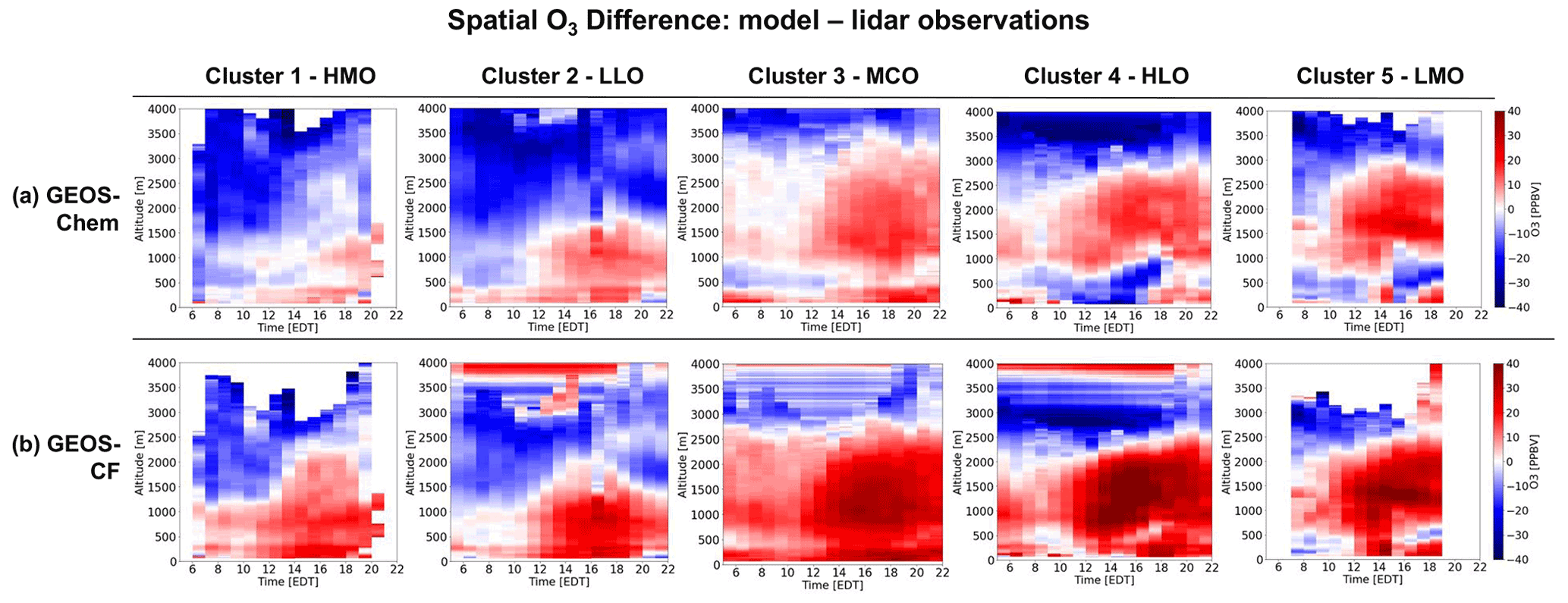
Figure 6 Mean profile curtain spatial O₃ difference (model–lidar observations) for each cluster (1–5). GEOS-Chem differences (a) and GEOS-CF differences (b).

For the mid-level, the overall correlation reveals that GEOS-CF and GEOS-Chem both have a weak relationship with the lidar (R=0.22 and R=0.12, respectively) (Fig. S7 – bottom panel, low level). This indicates that neither model can simulate the mid-level O₃ pattern well. GEOS-Chem consistently underestimates the magnitude of mid-level O₃ with a systematic high negative normalized bias ranging from −0.44 to −0.18, while GEOS-CF has a lower and non-systematic normalized bias ranging from −0.22 to 0.28. Overall, both models are unable to simulate the O₃ variability or magnitude well in the mid-level. The overall analysis provides a fundamental but condensed assessment of model performance.

Figure 7 O₃ correlation between lidar observations and (a) GEOS-Chem model simulation results and (b) GEOS-CF model results by each cluster split by low level (top rows) and mid-level (bottom rows).

3.3.2 Model evaluation based on lidar clusters

In this section we discuss significant cluster-by-cluster differences in model performance that are unmasked by the clustering approach. To better explain the side-by-side comparison in Fig. 4, spatial O₃ differences (model–lidar observations) for each cluster were derived (Fig. 6) as were individual cluster correlations (Fig. 7, Table S1). Subsequent mean normalized biases (Table S1) were calculated from the total vertical and diurnal averages separated by low level and mid-level.

In the low level, GEOS-CF has a similar performance ability for the HMO, HLO, and LMO clusters with high positive biases at +0.30, +0.41, and +0.45, respectively. These higher biases imply GEOS-CF has difficulty capturing moderate-O₃ cases (HMO and LMO) as well as high-O₃ cases (HLO) below 2000 m. GEOS-CF also has a high positive bias (+0.50) in the LLO cluster indicating the model struggles to capture the lower-O₃ cases as well. This is warranted as models are intended to approximate and are not usually able to capture extremes (high or low). In the low level, GEOS-Chem has the best performance (minimal −0.04 bias and strong correlation, R=0.61) in HLO, the cluster with the highest low-level O₃ accumulation, and the second-best performance (minimal +0.07 bias and fair correlation, R=0.55) in LLO, the cluster with the lowest O₃ accumulation. These results challenge the overall assumption that models struggle to capture extreme cases. GEOS-Chem has a similar performance for the LMO and HMO clusters with low negative biases of −0.10 and −0.09, respectively, indicating the model is also able to capture moderate-O₃ cases.

Both models perform the worst (in comparison to other clusters) in the low level in the MCO cluster with a +0.13 bias for GEOS-Chem and a +0.67 bias for GEOS-CF. As described in Sect. 3.1, MCO is the most common cluster with moderate–high average O₃ concentrations in the low level (refer to Fig. 3b). Although GEOS-Chem has its worst performance in the MCO cluster, it is not necessarily a poor performance. By contrast, the GEOS-CF performance in the MCO cluster reveals a more substantially high positive bias. This stands out as models are usually able to capture moderate levels (e.g., non-extreme cases). Evaluating the full temporal and vertical profile indicates that the higher GEOS-CF bias in the MCO cluster is additionally influenced by the greater overestimation of morning O₃, not solely the afternoon O₃. This is different to the performance in the LLO and LMO clusters where GEOS-CF also had a high positive bias in the low level but better simulates early morning O₃. A similar conclusion can be drawn when evaluating the low-level GEOS-Chem performance. HMO, LLO, MCO, and LMO all share “higher” biases (rounding to ± 0.10), but the highest bias is found in the MCO cluster. This can similarly be attributed to GEOS-Chem overestimating morning O₃ in the MCO cluster in contrast to the better early morning estimation in the other clusters.

In the mid-level, GEOS-Chem underestimates O₃ magnitude to the greatest extent in the HMO and the LLO cluster (both biases = −0.44), which are both clusters with higher mid-level O₃ concentrations (refer to Fig. 3c). GEOS-Chem performs similarly in the HLO and MCO clusters, with a negative mean bias of −0.30 and −0.27, respectively. This indicates that GEOS-Chem struggles most to simulate higher concentrations of O₃ in the mid-level. The GEOS-Chem model actually never reaches O₃ cluster averages greater than 50 ppb, directly divulging the greater systemic negative bias in the mid-level. GEOS-Chem simulates LMO mid-level O₃ magnitude the best (−0.18 bias), which is the cluster with the lowest O₃ average (< 45 ppb). Although for the LMO cluster GEOS-Chem has a lower bias, the correlation is still poor (R=0.23) which indicates that the model is relatively capable of simulating mid-level O₃ only when the case devises lower concentrations but still fails to replicate any O₃ variability and pattern.

On the other hand, GEOS-CF does best simulating LLO, MCO, and HLO, which are all clusters with moderate O₃ in the mid-level (≥ 50 and ≤ 70 ppb). GEOS-CF has the highest bias in the LMO cluster (+0.28), the cluster with the lowest mid-level O₃ magnitude, but also has the strongest correlation in the same cluster (R=0.74). This is a unique case where, although the model is not able to capture mid-level O₃ magnitude, it is able to capture the variability well. Comparing the full profile curtain, it is evident that in the LMO cluster, the GEOS-CF model simulates the mid-level O₃ pattern in the morning/early afternoon fairly well. GEOS-CF also struggles to simulate mid-level O₃ in the HMO cluster, by contrast the cluster with the highest mid-level O₃ (≥ 70 ppb). This supports the previous conclusion that, although GEOS-CF has a relatively lower biases in the mid-level, the model still struggles to simulate the extreme O₃ cases. Although GEOS-CF underestimates O₃ magnitude in the HMO cluster, it has a higher correlation than most of the other clusters (R=0.51) (Fig. 7, Table S1). GEOS-CF does a fair job connecting the mid-level higher O₃ pattern in the early morning that develops down to the low level later in the afternoon (Fig. 3). From this we can draw the conclusion that GEOS-CF is better able to capture mid-level O₃ patterns earlier in the temporal profile leading to better correlations with the lidar.

3.3.3 Advantages of the cluster approach and derived model conclusions

It is warranted that models struggle to simulate extreme events/cases such as seen in the low level in the HLO cluster and in the LLO cluster. However, GEOS-Chem performs best in both clusters with minimal biases and strong to fair correlations. Our results suggest that GEOS-Chem does a much better job simulating extreme O₃ cases in the low level than expected. We can conclude that the non-systemic bias is not only attributed to a good simulation of afternoon O₃ but also a fair simulation in morning O₃. This specific model feature is not eminent when evaluating overall performance. GEOS-CF systematically overestimates low-level O₃, but the individual clusters indicate that the model has a better correlation with O₃ in the HMO cluster. The higher O₃ levels measured throughout the diurnal profile from 1500–2000 m are well captured by the model and contribute to the better low-level correlation.

The clustering approach also reveals more discrepancies in the models such as in the MCO cluster. Evaluating the full profile curtains, we find that the overestimation of early morning O₃ in the low level in GEOS-CF adds to the systemic overestimation in afternoon O₃ contributing greater bias and poorer correlation. The same case can be found in the GEOS-Chem MCO cluster performance but to a lesser extent as GEOS-Chem has a much lower positive bias. Previous studies have found that excessive vertical mixing leads to overestimation of O₃ near the surface as well as underestimation of O₃ nighttime depletion resulting in overestimation of O₃ the next day (Dacic et al., 2020; Keller et al., 2021; Travis and Jacob, 2019). Model overestimation of O₃ at night and in the early morning hours is a common problem for 3-D Eulerian CTMs. Overnight, O₃ concentrations from the evening before can remain lingering in the residual layer. This residual layer sits at about 1000 m or higher depending on the conditions of the environment. O₃ trapped in this residual layer can directly correlate with the next day's afternoon O₃ (e.g., Fig. 3a; HLO cluster). Models struggle to resolve the shallow surface layer at night, which enhances nighttime NO titration and O₃ dry deposition. If this residual layer and the titration of O₃ overnight in the shallow surface layer are not resolved, next-day simulated O₃ will most likely warrant even greater biases. Therefore, in the given case where there is an O₃ event that lasts more than 1 d (at the same lidar location), the model will likely underestimate O₃ nighttime depletion, overpredict morning O₃, and subsequently overpredict the afternoon buildup. Given multiple cases of multi-day or consecutive high-O₃ events from the lidar measurements (17 total from HMO, MCO, and HLO), this is likely one of the reasons for GEOS-CF overestimating early and therefore afternoon O₃ in these high-O₃ cases in the low level. In Fig. 6, GEOS-CF exhibits the greatest afternoon O₃ overprediction in MCO and HLO. In HLO alone, there were 4 (out of 18) of the profiles that were consecutive while in MCO there were 8 (out of 28). This gives an explanation for upwards of 22 %–29 % of the overestimation of O₃ in the profile curtains of these clusters. These multi-day O₃ events are particularly important as they can indubitably lead models to overestimations of afternoon O₃. Full vertical and temporal curtains provided by lidar instruments are essential in fully understanding the development and depletion of O₃ in these cases. The mean curtain profiles in Fig. 3a indicate that what is captured at the surface (below 500 m) in the early morning does not represent what is captured in the residual layer (1000 m) by the lidar. Therefore, surface data would not be sufficient in evaluating a multi-day event.

GEOS-Chem does not have such an issue overestimating low-level O₃ in the afternoon. In the other clusters, GEOS-Chem actually underpredicts early morning low-level O₃ in the full vertical profile and does an overall better job than GEOS-CF simulating morning low-level O₃, such as in the HLO cluster. A better estimation of early morning O₃ does not warrant the same buildup of afternoon O₃. In these cases, GEOS-Chem handles the multi-day simulations better than GEOS-CF. This gives some explanation as to why GEOS-Chem underpredicts the other clusters with higher O₃ concentrations in the low level (HMO and HLO). GEOS-CF does best simulating morning low-level O₃ in cases of lower O₃ extent (LLO and LMO) but still overestimates the afternoon O_3. Since in these cases the afternoon does not seem to be related to early morning overestimations, other factors may be contributing. In the LLO cluster, the full curtain profile implies that excessive mixing throughout the entire vertical profile could be adding to afternoon O₃ overestimation. Similarly, for the LMO cluster, mid-level O₃ seems to be at play in influencing low-level O₃ which could be adding to afternoon biases.

In the mid-level GEOS-Chem consistently underestimates O₃ but the clusters reveal a better performance in LMO. It is evident that the model is better able to capture lower-magnitude O₃ cases in the mid-level. A unique case is exposed in which GEOS-CF has a strong correlation in the mid-level in the LMO cluster despite having a low correlation overall and in the other clusters. The individual cluster correlation reveals the GEOS-CF model is better able to capture the higher-O₃ observations in this cluster thus capturing more of the variability. Since the version of GEOS-Chem used in this study was run with the tropchem chemistry mechanism which excludes stratospheric chemistry (now obsolete with current GEOS-Chem developments) and GEOS-CF uses the UCX chemistry mechanism that includes stratospheric chemistry, this may allude to a better performance of GEOS-CF in simulating higher O₃ concentrations in the mid-level. The weak correlations in the mid-level could be due to multiple model inefficiencies such as the coarse model resolutions. Although GEOS-CF has a finer resolution than GEOS-Chem, it may still not be sufficient in horizontal and vertical grid resolution to replicate the O₃ variations captured in the 2-D lidar observations. Additionally, transport of emissions in the free troposphere (FT) is another influential factor that could contribute to the misrepresentation of mid-level O₃. In Fig. S8 in the Supplement, aircraft measurements from OWLETS-2 are used to evaluate GEOS-Chem-simulated carbon monoxide (CO) in the FT (1800–2500 $\mathrm{m}\mathrm{a}.\mathrm{g}.\mathrm{l}.$). The flight days evaluated are all curtain profiles that were assigned to the clusters with higher levels of O₃ in the mid-level (HMO, MCO, and HLO). It is evident that the model is able to capture lower levels of CO in the FT (100–110 ppbv) (e.g., background levels) but struggles to capture the higher levels (130–140 ppbv). Since increased levels of CO in the FT are indicative of possible long-range transport (Neuman et al., 2012), FT transport could be a factor contributing to the GEOS-Chem poor performance in the mid-level.

There are additional model discrepancies that can lead to underestimations of O₃ in GEOS-Chem in the mid-level that were found in all five clusters. One gap in the GEOS-Chem model could be the representation of tropospheric halogen chemistry which has a large effect on coastal O₃ production. Newer updates to the GEOS-Chem model (v12.9) have included updated tropospheric halogen chemistry mechanisms (iodine, bromine, and chlorine) (Wang et al., 2021) and indicate that further investigation of halogen chemistry is needed for better model representation. Another study finds a similar conclusion in the proper representation of cloud uptake and tropospheric chemistry in the model (Holmes et al., 2019), warranting further testing. The role lightning plays in tropospheric oxidation is another feature that is commonly misrepresented in global models and can affect O₃ simulation (Mao et al., 2021). These are all examples of features that if not simulated correctly can lead to misestimations of O₃. The clustering approach allows us to organize the detailed lidar measurements to scope out specific cases where these misrepresentations occur. These previous studies also highlight the importance of lidar measurements and their ability to depict tropospheric emission development and behavior throughout the vertical profile and diurnal cycle which can be used to constrain model emissions and improve simulations.

Although this analysis proves to be a useful technique to characterize the largely variably O₃ behavior in coastal regions and evaluate the subsequent model performance, there are also limitations. In this study we are comparing single-point lidar versus model output; therefore we cannot simply state that the model is incorrect. We make conclusions and calculate biases based on the ability to subset a grid point and compare that to a single-point lidar curtain to our best ability, but that still leaves an uncertainty.

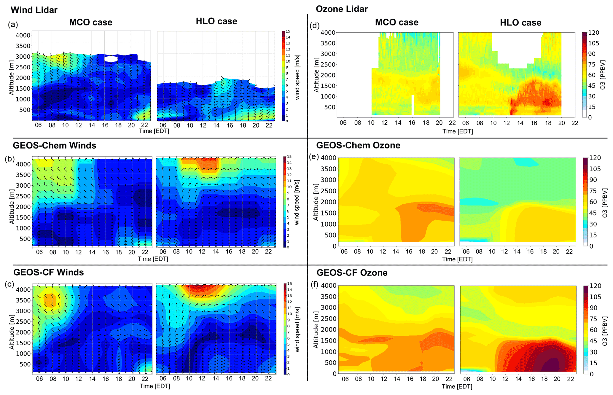
Figure 8 Profile curtains of wind speed/direction (a–c) and O₃ (d–f) from the lidar (a, d), GEOS-Chem (b, d), and GEOS-CF (c, f). Results from OWLETS-2 at HMI. Wind direction is depicted by wind barbs. The white spaces indicate missing data for both the (a) wind and (d) O₃ lidar curtain profiles.

3.4 Cluster-derived case studies to evaluate modeled wind and ozone

Meteorological factors such as wind speed and direction can directly impact whether a coastal region will experience clean air or O₃ exceedances. When local meteorological processes such as sea/bay breeze occur at such a fine scale, equally fine-resolution measurements are essential in capturing this. The Doppler wind lidar offers a focus on fine details that are only revealed in the multi-dimensional data, which allows for such a comprehensive evaluation of the established O₃ cluster profile curtains. In this section, we evaluate the 2-D relationship between wind and O₃ to assess model performance using lidar and model-derived profile curtains (Fig. 8). We derived two specific case studies, each from a different cluster: MCO, 17 June 2018, and HLO, 30 June 2018. Utilizing the derived clusters, the case studies were chosen to focus on high low-level O₃ behavior cases with a goal of evaluating possible sea/bay breeze events. The two case studies are both from the HMI location during the OWLETS-2 campaign. The white spaces in both the wind and O₃ lidar figures (Figs. 4, 6, and 8) indicate missing data.

3.4.1 Sea breeze event interpretation

In the MCO case, the Doppler wind lidar captures a wind direction shift from westerly to easterly winds beginning at 06:00 EDT accompanied by calm winds (approximately 0 m s⁻¹) indicating an early onset sea/bay breeze event. The timing of the start of this event is simulated well. but the models fail to predict an actual well-defined wind shift, instead merely simulating 0 m s⁻¹ winds after 05:00 EDT. A wind direction shift is depicted in the HLO case, with westerly winds early in the morning and a shift to southeasterly winds later in the temporal profile (at about 10:00 EDT). This could also likely be a common sea breeze event which could have contributed to the high observed O₃ concentrations in the afternoon. Again, the exact timing of the start of the wind shift is captured by the models, but then no defined directional shift and little to no winds are simulated afterwards, with a worse performance for the GEOS-Chem model. Based on the Doppler wind lidar curtain profiles, we can derive the conclusion that the two sea/bay breeze cases are distinct. The HLO case closely mirrors a common sea/bay breeze event with a more definite wind direction shift later in the morning and winds above the surface remain consistent throughout the profile. The MCO case shows a less discernible wind shift which also begins earlier in the morning with weaker winds above the surface. These differences are not well captured by either model. It is important to note that GEOS-Chem runs with offline meteorology, averaged every 3 h. Since sea/bay breezes often happen at a finer temporal resolution, the GEOS-Chem model is at a disadvantage in modeling such fine processes.

3.4.2 Wind relation to ozone cases and clustering

In this sect., the wind lidar curtains will be assessed in relation to the O₃ lidar profile curtains and the model performance. We show in Sect. 3.3.2 that both models have the highest bias and lowest correlation simulating low-level O₃ in the MCO cluster. Mirroring those results, both models overestimate low-level O₃ in the MCO case studies (Fig. 8e and f). Higher O₃ concentrations are captured in the lidar curtain profile throughout the day but are constrained between 1000–2000 m. Both models bring this high-O₃ pattern down to the surface (below 500 m), which contributes to the overestimation. The models predict little to no winds in the low level simulating a stagnant environment. Simulated stagnant winds reflect lower dilution rates and induce higher O₃ concentration buildup near the surface that is reproduced in both models. For the mid-level, the GEOS-CF model seems to replicate the O₃ pattern better, while GEOS-Chem overestimates O₃. This is a unique finding that was not detected in the previous analysis, where GEOS-Chem was found to consistently underestimate mid-level O₃. From the data available above 2000 m, both models seem to do well replicating mid-level winds. This implies that there are more factors at play such as transport or background level O₃ that may have prompted the overestimated O₃ in these cases.

For the HLO cluster, GEOS-CF had a high positive mean normalized bias and a reasonable relationship (R=0.61) in the low level (Sect. 3). For the individual HLO case (Fig. 8f), GEOS-CF was similarly found to overestimate low-level O₃ magnitude, while it is better able to capture the O₃ pattern. GEOS-CF is better able to reproduce the wind shift in HLO (Fig. 8c), but, like the MCO case, stagnant winds simulated earlier in the morning suggest a similar overestimation of early morning O₃. This is another clear example supporting the tendency for GEOS-CF to overestimate morning O₃ which can facilitate an overestimation in the afternoon. The GEOS-Chem HLO case results mirror its mean cluster performance closely by underestimating both low-level and mid-level O₃. For this case, the simulated winds indicate a very different result than the lidar winds, simulating no winds in the low level for almost the entirety of the temporal profile and vertical profile. Since the results reveal O₃ is underestimated, this suggests that there are more factors affecting O₃ results in this specific case. One of these factors can be the simulation of the boundary layer as the sea/bay breeze develops. If the boundary layer is simulated to be larger in depth, the ability for the model to simulate higher O₃ concentrations may be hindered, such as found in Dacic et al. (2020). Since the HLO case indicates a common sea breeze event based on the timing and shift, it appears that GEOS-Chem really struggles to capture this intricate process while GEOS-CF does a better job.

It is evident from these cases that differences in sea/bay breeze events can lead to diverse O₃ profiles. The HLO case has high O₃ levels that reach down to the surface, with peaks >75 ppb at both 12:00 and again at 16:00 EDT. Just above this extreme O₃ plume at 2000 m, there is an O₃ deficit of almost 50 ppb. The MCO case differs in that the highest O₃ concentrations do not reach the surface. Also, O₃ is more distributed and mixed throughout the curtain profile, and the vertical gradient, although present, is not as stark as in the HLO case. The HLO case also has higher O₃ captured aloft above 2500 m, which is not captured in the MCO case. Analyzing their full curtain profiles, it is easy to conclude why these events were not assigned to the same cluster and the differences are also apparent in the individual model performance. For both cases, the models generally seem to underestimate wind speed and overestimate O₃ (to different extents) but the GEOS-Chem performance in the HLO case is different. The uniqueness of this case implies that GEOS-Chem struggles to simulate this sea/bay breeze based on factors other than wind speed and direction.

It is imperative to correctly simulate coastal mechanisms in order to mitigate high-O₃ events. To accurately simulate such complex exchanges, high-resolution vertical and horizontal simulations are needed. Because of the models' relatively coarse resolutions (nominally 50 and 25 km horizonal resolution; 72 vertical levels), the fine-scale vertical wind gradients and horizontal wind shifts are difficult to resolve and, in these cases, not fully possible to replicate. This study also acknowledges the need for an evaluation of other modeled factors, aside from model resolution, such as divulged in Sect. 3.3.3, considering the possible confounding effects on modeled O₃ outcome.

4 Conclusion

We developed a clustering method based on a suite of 91 multi-dimensional lidar O₃ profile curtains retrieved from three recent campaigns. The K-means clustering algorithm, driven by eight well-defined features, was applied to categorize the fine-resolution O₃ data, revealing five distinct O₃ behavior cases that all vary in pattern and magnitude vertically and temporally. The results indicate that fine-resolution data can be used to characterize highly variable vertical and temporal coastal O₃ behavior and classify different cases of O₃ exploiting the multiple dimensions. Furthermore, this approach could be used by states to better identify different O₃ photochemical regimes and frequency beyond just surface sampling.

The performance of two CTMs (GEOS-Chem and GEOS-CF) was evaluated. Overall, the models had a weak overall relationship with the lidar observations in the mid-level (R=0.12 and 0.22). GEOS-Chem had a systematic high negative bias and GEOS-CF had an overall lower unsystematic bias range. In the low level, GEOS-Chem had an low unsystematic bias range and fair relationship with the lidar observations (R=0.66), while GEOS-CF had a systematic high positive bias but overall fair relationship (R=0.69). Utilizing the curated clusters reveals new model insight that is neglected in the overall performance analysis. GEOS-Chem does best simulating extreme O₃ cases in the low level (such as in HLO and LLO). The greater underestimations of mid-level O₃ for GEOS-Chem can be attributed to multiple model discrepancies such as the mechanism used (tropchem), which only considers tropospheric chemistry. Another factor inhibiting the poor simulation in the mid-level is the model failing to capture long-range transport of emissions in the FT. Evaluating the full profile curtains reveal that GEOS-CF low-level overestimations can be most attributed to the greater overestimation of early morning O₃. This feature is affiliated with multi-day O₃ events where O₃ lingering in the residual layer overnight can contribute to higher O₃ in the afternoon the next day and proves to be a challenge for CTMs. Lidar curtain profiles prove to be essential in evaluating these multi-day cases as they can capture the full development and deposition of O₃ in the residual layer that is not observed at the surface. Although we find that the GEOS-CF model struggles to simulate O₃ magnitude in the mid-level, it can relatively emulate O₃ variability in some cases (LMO cluster). GEOS-CF also does fairly well in cases in which the pattern of higher mid-level O₃ suggests a relationship with the low-level O₃. Although GEOS-CF is run with the combined tropospheric and stratospheric chemistry mechanism, has a finer grid resolution, and is an online model, we conclude there are still limitations to both models which contribute to the difficulty in simulating fine-scale coastal O₃ variability.

We demonstrate a unique value of the clustering approach on multi-dimensional lidar data in which we use the cluster results to evaluate two cases studies from the MCO and HLO clusters. The wind speed and directional shifts (onshore to offshore) illustrated in wind lidar profile curtains indicate a possible sea/bay breeze event in both case studies. The two cases represent distinct sea/bay breeze events that lead to different O₃ developments that were difficult for the CTMs to reproduce, due to coarse model resolution and other possible factors. With a regional model analysis being outside the scope of this study, we propose to use multi-dimensional lidar measurements to evaluate finer regional modeling in our future work.

This work is the first time that all three associated campaign lidar data have been analyzed in conjunction. The value of lidar measurements is reflected in their ability to reveal unique features within the temporal and vertical pattern of O₃ behavior. Applying the clustering analysis directly to the lidar O₃ data emerges as a useful and robust approach for identifying O₃ regimes. Further observations using lidar instruments should be especially valuable in investigating coastal O₃ behavior as it can divulge the finer-scale O₃ characteristics that remain difficult to successfully simulate in CTMs. We provide a new approach that is the middle ground between looking at specific cases and summarizing overall model performance that allows a synopsis of summer coastal O₃ behavior and subsequently model performance without completely muting distinct O₃ features. Evaluating model performance for diverse O₃ behavior in coastal regions is crucial for improving the simulation and, furthermore, mitigation of air quality events.