Intermittency of gravity wave potential energies and absolute momentum fluxes derived from infrared limb sounding satellite observations

Atmospheric gravity waves contribute significantly to the driving of the global atmospheric circulation. Because of their small spatial scales, their effect on the circulation is usually parameterized in general circulation models. These parameterizations, however, are strongly simplified. One important but often neglected characteristic of the gravity wave distribution is the fact that gravity wave sources and, thus, the global distribution of gravity waves are both very intermittent. Therefore, time series of global observations of gravity waves are needed to study the distribution, seasonal variation, and strength of this effect.

For gravity wave absolute momentum fluxes and potential energies observed by the High-Resolution Dynamics Limb Sounder (HIRDLS) and Sounding of the Atmosphere using Broadband Emission Radiometry (SABER) limb sounding satellite instruments, we investigate the global distribution of gravity wave intermittency by deriving probability density functions (PDFs) in different regions as well as global distributions of Gini coefficients. In the stratosphere, we find that intermittency is strongest in mountain wave regions, followed by the polar night jets and by regions of deep convection in the summertime subtropics. Intermittency is weakest in the tropics. A better comparability of intermittency in different years and regions is achieved by normalizing observations by their spatially and temporally varying monthly median distributions. Our results are qualitatively in agreement with previous findings from satellite observations and quantitatively in good agreement with previous findings from superpressure balloons and high-resolution models. Generally, momentum fluxes exhibit stronger intermittency than potential energies, and lognormal distributions are often a reasonable approximation of the PDFs. In the tropics, we find that, for monthly averages, intermittency increases with altitude, which might be a consequence of variations in the atmospheric background and, thus, varying gravity wave propagation conditions. Different from this, in regions of stronger intermittency, particularly in mountain wave regions, we find that intermittency decreases with altitude, which is likely related to the dissipation of large-amplitude gravity waves during their upward propagation.

1 Introduction

Atmospheric waves are important drivers of the atmospheric circulation (e.g., Andrews et al., 1987, and references therein). Particularly, the global observation and modeling of gravity waves is very challenging because of their small spatial scales (e.g., Fritts and Alexander, 2003, and references therein). In the middle atmosphere, typical horizontal wavelengths of gravity waves are in the range of a few tens of kilometers to a few thousand kilometers. Their vertical wavelengths range from below 1 km to several tens of kilometers (e.g., Preusse et al., 2008; Alexander et al., 2010, and references therein).

Many gravity wave sources are located in the troposphere and lower stratosphere. Some of the most relevant gravity wave sources are atmospheric flow over topography (e.g., McFarlane, 1987; Lott and Miller, 1997; Eckermann and Preusse, 1999; Kruse et al., 2022), deep convection (e.g., Fovell et al., 1992; Pfister et al., 1993; Piani et al., 2000; Song and Chun, 2005; Stephan et al., 2019a, b; Ern et al., 2022), and processes related to strong wind jets and fronts (e.g., Charron and Manzini, 2002; Zhang, 2004; Zülicke and Peters, 2006; Plougonven and Zhang, 2014; Kim et al., 2016; Wei et al., 2016; Geldenhuys et al., 2021). According to their sources, these waves are also called mountain waves (or orographic gravity waves), convective gravity waves, and jet- or front-generated gravity waves, respectively.

Gravity waves propagate away from their sources, both vertically and horizontally, redistributing energy and momentum in the atmosphere and, thus, coupling different atmospheric layers and regions. When gravity waves dissipate, they exert forcing (“gravity wave drag”) on the atmospheric background flow (e.g., McLandress, 1998; Fritts and Alexander, 2003).

The vertical flux of horizontal pseudomomentum of a gravity wave (denoted as “momentum flux” in the following for simplification) is given by

$$\begin{array}{}\text{(1)}& (F_{px},F_{py})=\stackrel{\mathrm{‾}}{\mathit{\varrho }}(\mathrm{1}-{\displaystyle \frac{f^{\mathrm{2}}}{{\widehat{\mathit{\omega }}}^{\mathrm{2}}}})(\stackrel{\mathrm{‾}}{u^{\prime }{w}^{\prime }},\stackrel{\mathrm{‾}}{v^{\prime }{w}^{\prime }})\end{array}$$

(e.g., Fritts and Alexander, 2003), where F_px and F_py are the zonal and the meridional momentum flux, respectively; $\stackrel{\mathrm{‾}}{\mathit{\varrho }}$ is the atmospheric background density; f is the Coriolis frequency; $\widehat{\mathit{\omega }}$ is the intrinsic frequency of the gravity wave; and u^′, v^′, and w^′ are the wind perturbations of the background atmosphere in the zonal, meridional, and vertical directions, respectively, that are caused by the gravity wave. Averaging over one or multiple full wave cycles is indicated by the overbars. The absolute momentum flux F_ph of a gravity wave is given by

$$\begin{array}{}\text{(2)}& F_{ph}=\sqrt{F_{px}^{\mathrm{2}}+F_{py}^{\mathrm{2}}},\end{array}$$

and the gravity wave drag (X,Y) that a gravity wave exerts on the background flow is given by

$$\begin{array}{}\text{(3)}& (X,Y)=-{\displaystyle \frac{\mathrm{1}}{\stackrel{\mathrm{‾}}{\mathit{\varrho }}}}{\displaystyle \frac{\partial (F_{px},F_{py})}{\partial z}},\end{array}$$

where X and Y are the gravity wave drag in zonal and meridional directions, respectively, and z is the vertical coordinate.

Gravity waves contribute significantly to the driving of the meridional circulation in the stratosphere (e.g., Alexander and Rosenlof, 2003) and in the mesosphere (e.g., Holton, 1983). They are the main drivers of the wind reversal at the top of the mesospheric wind jets in both the summer hemisphere and the winter hemisphere (e.g., Lindzen, 1981; Holton, 1982). Gravity wave drag is also an important contribution to the zonal momentum budget in the tropics, and, along with global-scale waves, they drive the quasi-biennial oscillation (QBO) (e.g., Lindzen and Holton, 1968; Ern and Preusse, 2009a, b; Alexander and Ortland, 2010; Ern et al., 2014) and the semiannual oscillation (SAO) (e.g., Delisi and Dunkerton, 1988; Antonita et al., 2007; Ern et al., 2015, 2021; Smith et al., 2022) of the zonal wind in the tropics. Further, gravity waves contribute to the variations in the polar night jets around sudden stratospheric warmings (SSWs) (e.g., Hitchcock and Shepherd, 2013; Albers and Birner, 2014; Ern et al., 2016) and contribute to the forcing of global-scale waves in the mesosphere (e.g., Holton, 1984; Smith, 2003; Ern et al., 2013; Matthias and Ern, 2018; Sato et al., 2018).

Another important effect is that temperature fluctuations of gravity waves contribute to the formation of ice clouds and, thus, dehydration in the upper troposphere and the tropopause region (e.g., Schoeberl et al., 2015; Dinh et al., 2016), as well as to the formation of polar stratospheric clouds (e.g., Carslaw et al., 1999; Eckermann et al., 2009), and, thus, to ozone depletion in the polar regions (e.g., Orr et al., 2020, and references therein).

General circulation models (GCMs) and chemistry climate models (CCMs) usually resolve only parts of the whole spectrum of gravity waves. Therefore, the effect of gravity waves on the global circulation is simulated by gravity wave parameterizations (e.g., Fritts and Alexander, 2003; Kim et al., 2003; Geller et al., 2013, and references therein). These gravity wave parameterizations are usually very simplified. For example, they assume that gravity waves propagate only vertically, whereas gravity waves in the real atmosphere can propagate not only vertically but also horizontally (e.g., Sato et al., 2009; Preusse et al., 2009b; Kalisch et al., 2014; Hindley et al., 2015; Thurairajah et al., 2017).

Several parameterizations exist that are dedicated to specific gravity wave source processes. Some examples are McFarlane (1987) or Lott and Miller (1997) for mountain waves; Charron and Manzini (2002) or de la Cámara and Lott (2015) for gravity waves excited by jets and fronts; and Beres et al. (2004), Song and Chun (2005), or Bushell et al. (2015) for convectively generated gravity waves. Many gravity wave parameterizations, however, comprise the contribution of non-orographic gravity waves into just one parameterization that assumes a globally constant (e.g., Warner and McIntyre, 2001; Orr et al., 2010), piecewise constant (e.g., Molod et al., 2015), or otherwise very simplified source distribution, even though it is evident that a more realistic middle atmosphere can be simulated by more realistic gravity wave source distributions (e.g., de la Cámara et al., 2014; Yigit et al., 2021).

While orographic gravity wave parameterizations can simulate a highly intermittent gravity wave distribution (e.g., Kuchar et al., 2020; Sacha et al., 2021) because they are driven by the highly variable near-surface winds, these simplified non-orographic gravity wave parameterizations are not coupled to realistic specific source processes. Therefore, they do not account for the intermittency of gravity wave sources and the resulting intermittent global distributions of gravity waves. In the real atmosphere, gravity wave amplitudes, wavelengths, and momentum fluxes can vary strongly, both spatially and temporally. Particularly, large-amplitude gravity waves will saturate earlier and exert their drag at different locations than small-amplitude gravity waves (e.g., Fritts, 1984). As a consequence, if uniform and constant launch amplitudes are assumed, the resulting global distribution of gravity wave drag will not be fully realistic.

To overcome this limitation, several gravity wave parameterizations simulate the intermittency of gravity wave sources by introducing stochastic variations in the gravity wave sources (e.g., Eckermann, 2011; Lott et al., 2012; de la Cámara et al., 2014; de la Cámara and Lott, 2015; Serva et al., 2018). It has been shown, for example, by de la Cámara et al. (2014) that this can lead to more realistic simulations of the QBO and that the gravity wave forcing at the top of the mesospheric wind jets does not unrealistically peak around a single altitude but rather over a range of altitudes, including also somewhat lower altitudes.

Generally, parameterizations need guidance by observations to become more realistic. Consequently, observations of gravity waves and their intermittency are needed to improve stochastic gravity wave parameterizations. In addition, these kind of observations are needed for comparison with gravity wave parameterizations that are dedicated to specific source processes, like orography and convection, as well as for comparison with gravity waves that are explicitly resolved by high-resolution models. Some examples of gravity wave intermittency observations from ground-based stations are Zink and Vincent (2001), Cao and Liu (2016), Minamihara et al. (2020), or Conte et al. (2022). Gravity wave intermittency has also been studied using superpressure balloon observations in the Southern Hemisphere at polar latitudes (Hertzog et al., 2008, 2012; Plougonven et al., 2013; Jewtoukoff et al., 2015) as well as in the tropics (Jewtoukoff et al., 2013; Corcos et al., 2021). Further, gravity wave intermittency has been derived from satellite observations, for example, from Global Navigation Satellite System radio occultations (GNSS-RO) (Baumgaertner and McDonald, 2007), from High-Resolution Dynamics Limb Sounder (HIRDLS) observations (Hertzog et al., 2012; Wright et al., 2013), and from nadir soundings of the Atmospheric Infrared Sounder (AIRS) instrument (Alexander and Grimsdell, 2013; Wright et al., 2017).

In our study, we determine gravity wave intermittency for monthly global distributions of gravity wave potential energies and absolute momentum fluxes derived from observations of the HIRDLS and Sounding of the Atmosphere using Broadband Emission Radiometry (SABER) limb sounding satellite instruments. Compared with previous estimates of gravity wave intermittency from limb sounders, our data cover a larger range of gravity wave vertical wavelengths. In addition, SABER observations cover a larger altitude range, including the whole mesosphere. This allows one to follow the evolution of gravity wave intermittency from the middle stratosphere (close to the gravity wave sources) to the upper mesosphere (where gravity waves strongly dissipate and drive the reversal of the mesospheric wind jets).

The remainder of the paper is structured as follows: the HIRDLS and SABER instruments are briefly introduced in Sect. 2; in Sect. 3, we describe how gravity wave potential energies and absolute momentum fluxes are derived; in Sect. 4, gravity wave intermittency is discussed based on probability density functions (PDFs); in Sect. 5, we introduce the Gini coefficient for investigating global distributions of intermittency in the stratosphere with better spatial resolution; using distributions of Gini coefficients, the evolution of intermittency in the vertical direction is investigated in Sect. 6; and, finally, Sect. 7 provides a summary and discussion.

2 The HIRDLS and SABER satellite instruments

The HIRDLS and SABER satellite instruments observe Earth's atmosphere in limb-viewing geometry. HIRDLS was launched onboard the Earth Observing System (EOS) Aura satellite and provided observations from 22 January 2005 until 17 March 2008 in the latitude range from about 63^∘ S to 80^∘ N. SABER was launched onboard the Thermosphere Ionosphere Mesosphere Energetics and Dynamics (TIMED) satellite and started atmospheric observations on 25 January 2002. SABER measurements are still ongoing at the time of writing. The TIMED satellite performs yaw maneuvers approximately every 60 d. As a consequence, SABER changes between a northward-viewing and a southward-viewing measurement geometry about every 60 d. The latitude coverages are about 50^∘ S to 82^∘ N and about 82^∘ S to 50^∘ N, respectively. Therefore, the latitude coverage of monthly averages is either 50^∘ S to 82^∘ N or 82^∘ S to 50^∘ N for those months not containing a yaw maneuver, or, in the case of months containing a yaw, 82^∘ S to 82^∘ N but with coverage at high latitudes only during part of the month. Initially, yaws were performed during “odd” months (i.e., January, March, May, July, September, and November), but the times of the yaw maneuvers have gradually shifted during the SABER mission.

While both instruments observe several atmospheric trace species, our work focuses on HIRDLS and SABER temperature observations. Both instruments are infrared radiometers, and atmospheric temperatures are derived from infrared emissions of CO₂ at around 15 µm. Because both instruments are limb sounders, they provide temperature altitude profiles with good vertical resolution. The vertical resolution is about 1 km for HIRDLS (∼2 km above 60 km altitude) and about 2 km for SABER. The altitude range of HIRDLS temperatures is from about the tropopause to near the mesopause. The SABER instrument was designed for observations at even higher altitudes, and temperatures cover the altitude range from about the tropopause to well above 100 km.

A description of the HIRDLS instrument is given in Gille et al. (2003), and the HIRDLS temperature retrieval is described in Gille et al. (2008, 2011). The SABER instrument is described in more detail in Mlynczak (1997) and Russell et al. (1999). More information on the SABER temperature retrieval can be found in Remsberg et al. (2004, 2008).

3 Gravity wave analysis based on satellite limb soundings

3.1 Determination of gravity wave temperature fluctuations

Observed temperature altitude profiles are a superposition of the large-scale atmospheric background and of the temperature fluctuations due to gravity waves. We isolate the temperature fluctuations due to gravity waves by following the approach described in Ern et al. (2018). First, from each altitude profile a zonal mean altitude profile is subtracted. The resulting altitude profiles of residual temperatures still contain the contributions of both global-scale waves and gravity waves.

The contribution of global-scale waves is determined by a dedicated spectral analysis (Ern et al., 2011). The 2D spectra in longitude and time are calculated in overlapping 31 d time windows for a set of fixed altitudes and latitudes. The contribution of global-scale waves is determined for each observation in every altitude profile from these spectra for the respective location (i.e., longitude, latitude, and height) and time. This approach removes global-scale waves with periods as short as about 1.3 d and covers 2 d waves, tropical Kelvin waves, and inertial instabilities that are difficult to remove by other methods (e.g., Ern et al., 2008, 2009; Ern et al., 2013; Rapp et al., 2018; Strube et al., 2020). Additional high-pass filtering was applied separately to each altitude profile in order to limit the range of vertical wavelengths still contained in each altitude profile to shorter than about 25 km. This high-pass filtering is performed by fitting and subtracting a sinusoidal wave with a vertical wavelength of 40 km or longer, individually for each altitude profile. In this way, remnants of global-scale waves are further reduced, and the range of gravity wave vertical wavelengths is limited to the range that is suitable for the momentum flux analysis described in Sect. 3.2.

In an additional step, atmospheric tides are removed from the temperature residuals. For satellites in slowly precessing low-Earth orbits, solar tides appear as wave patterns that are stationary if ascending (satellite flying northward), and descending (satellite flying southward) orbit parts are considered separately in time intervals that are much shorter than the period of one full satellite precession cycle. The reason for this is that, during these short time intervals, the respective local solar times of the ascending and descending parts of the satellite orbit are about constant. This fact is utilized to remove tides up to apparent zonal wave number 4 from observed altitude profiles (Ern et al., 2013).

After performing the abovementioned steps, the resulting altitude profiles of residual temperatures can be attributed mainly to gravity waves. An approximation for the sensitivity of limb sounding satellite instruments to gravity waves was derived by Preusse et al. (2002) as a function of the gravity wave horizontal and vertical wavelength. Approximate sensitivity functions that apply to the HIRDLS and SABER datasets used here are given in Ern et al. (2018).

3.2 Gravity wave potential energies and absolute momentum fluxes

The gravity wave potential energy E_pot is given by

$$\begin{array}{}\text{(4)}& E_{\mathrm{pot}}={\displaystyle \frac{\mathrm{1}}{\mathrm{2}}}{\left({\displaystyle \frac{g}{N}}\right)}^{\mathrm{2}}\stackrel{\mathrm{‾}}{{\left({\displaystyle \frac{T^{\prime }}{\stackrel{\mathrm{‾}}{T}}}\right)}^{\mathrm{2}}},\end{array}$$

where T^′ is the temperature fluctuations due to the gravity wave, g is the gravity acceleration, N is the buoyancy frequency, and $\stackrel{\mathrm{‾}}{T}$ is the atmospheric background temperature. Using the gravity wave temperature amplitude $\widehat{T}$, this can be rewritten as follows:

$$\begin{array}{}\text{(5)}& E_{\mathrm{pot}}={\displaystyle \frac{\mathrm{1}}{\mathrm{4}}}{\left({\displaystyle \frac{g}{N}}\right)}^{\mathrm{2}}{\left({\displaystyle \frac{\widehat{T}}{\stackrel{\mathrm{‾}}{T}}}\right)}^{\mathrm{2}}.\end{array}$$

The reader is also referred to Ern et al. (2018).

For deriving gravity wave absolute momentum fluxes from temperature observations, Eq. (1) has to be rewritten in terms of gravity wave temperature amplitudes using the linear gravity wave polarization relations (Ern et al., 2004; Ern et al., 2017):

$$\begin{array}{}\text{(6)}& (F_{px},F_{py})={\displaystyle \frac{\mathrm{1}}{\mathrm{2}}}\stackrel{\mathrm{‾}}{\mathit{\varrho }}{\left({\displaystyle \frac{g}{N}}\right)}^{\mathrm{2}}{\displaystyle \frac{(k,l)}{m}}{\left({\displaystyle \frac{\widehat{T}}{\stackrel{\mathrm{‾}}{T}}}\right)}^{\mathrm{2}}.\end{array}$$

This involves the 3D gravity wave wave vector, where k, l, and m represent the zonal, meridional, and vertical wave numbers, respectively. For gravity wave absolute momentum fluxes, we obtain

$$\begin{array}{}\text{(7)}& F_{ph}={\displaystyle \frac{\mathrm{1}}{\mathrm{2}}}\stackrel{\mathrm{‾}}{\mathit{\varrho }}{\left({\displaystyle \frac{g}{N}}\right)}^{\mathrm{2}}{\displaystyle \frac{{\mathit{\lambda }}_z}{{\mathit{\lambda }}_h}}{\left({\displaystyle \frac{\widehat{T}}{\stackrel{\mathrm{‾}}{T}}}\right)}^{\mathrm{2}},\end{array}$$

where $k_h={\left(k^{\mathrm{2}}+l^{\mathrm{2}}\right)}^{\mathrm{0.5}}=\mathrm{2}\mathit{\pi }/{\mathit{\lambda }}_h$ is the horizontal wave number of the gravity wave, λ_h is its horizontal wavelength, and λ_z is its vertical wavelength.

For each observed vertical profile of residual temperatures, we carry out a combination of the maximum entropy method (MEM) and harmonic analysis (HA), following Preusse et al. (2002), to derive altitude profiles of gravity wave amplitudes, vertical wavelengths, and phases for the strongest wave component at each altitude, based on running 10 km vertical windows. These gravity wave amplitudes are used to calculate gravity wave potential energies after Eq. (5). This can be performed for each altitude profile.

The estimation of gravity wave absolute momentum fluxes is more difficult because the gravity wave horizontal wavelength λ_h has to be estimated. For gravity wave momentum fluxes, we follow the approach of Ern et al. (2004, 2011) and focus on pairs of altitude profiles along the satellite measurement track that are not horizontally separated by more than about 300 km. For these pairs of altitude profiles, we determine the vertical phase difference of the strongest wave at each altitude. From these phase differences, the apparent horizontal wavelength of a gravity wave parallel to the satellite measurement track can be estimated. For an illustration see, for example, Preusse et al. (2009a) and Ern et al. (2018).

We assume that the same wave is seen in both altitude profiles if the vertical wavelengths in the two profiles differ by no more than 40 %. All other pairs of altitude profiles are discarded (i.e., those with nonmatching vertical wavelengths and those that have overly large distances between the two profiles). The remaining pairs of altitude profiles are likely still representative of the whole distribution of gravity waves, because distributions of squared gravity wave amplitudes of the remaining pairs are approximately equal to the distributions calculated from single altitude profiles and also approximately equal to the distributions calculated from the unused pairs of altitude profiles (see also Ern et al., 2018).

Absolute momentum fluxes are calculated by assuming that the horizontal wavelength parallel to the measurement track can be used as a proxy for the true horizontal wavelength of a gravity wave. Because the horizontal wavelength parallel to the measurement track will always overestimate the true horizontal wavelength, this will introduce large biases and likely result in an underestimation of absolute momentum fluxes. Other error sources are aliasing effects caused by an undersampling of observed gravity waves and effects caused by the instrument sensitivity functions. Both of these effects could cause an even stronger underestimation of absolute momentum fluxes. The full observational filter of limb sounding satellite instruments is discussed in more detail by, for example, Trinh et al. (2015) or Trinh et al. (2016). Overall errors in the momentum fluxes derived in this manner are at least a factor of 2 (see also Ern et al., 2004; Ern et al., 2017, 2018).

As an example, Fig. 1 shows global distributions of gravity wave potential energies for the HIRDLS instrument at an altitude of 30 km for each calendar month. The time range used for averaging is from March 2005 until February 2008. The global distributions were gridded using overlapping 5^∘ × 15^∘ (latitude × longitude) bins, and each bin slid 2.5^∘ in latitude and 5^∘ in longitude to yield a final 2.5^∘ × 5^∘ (latitude × longitude) grid. Figure 2 shows the same as Fig. 1 but for the SABER instrument using an averaging period from January 2002 until October 2020 and, as SABER has a coarser sampling resolution, larger latitude × longitude bins of 10^∘ × 15^∘ are used with the same final 2.5^∘ × 5^∘ grid. Different from the global distributions shown in Ern et al. (2018), values are multiyear means of medians, not multiyear means of the arithmetic mean values. Further, for each single month entering the multiyear means, grid points are not used if fewer than 40 data points are contained in the respective grid box.

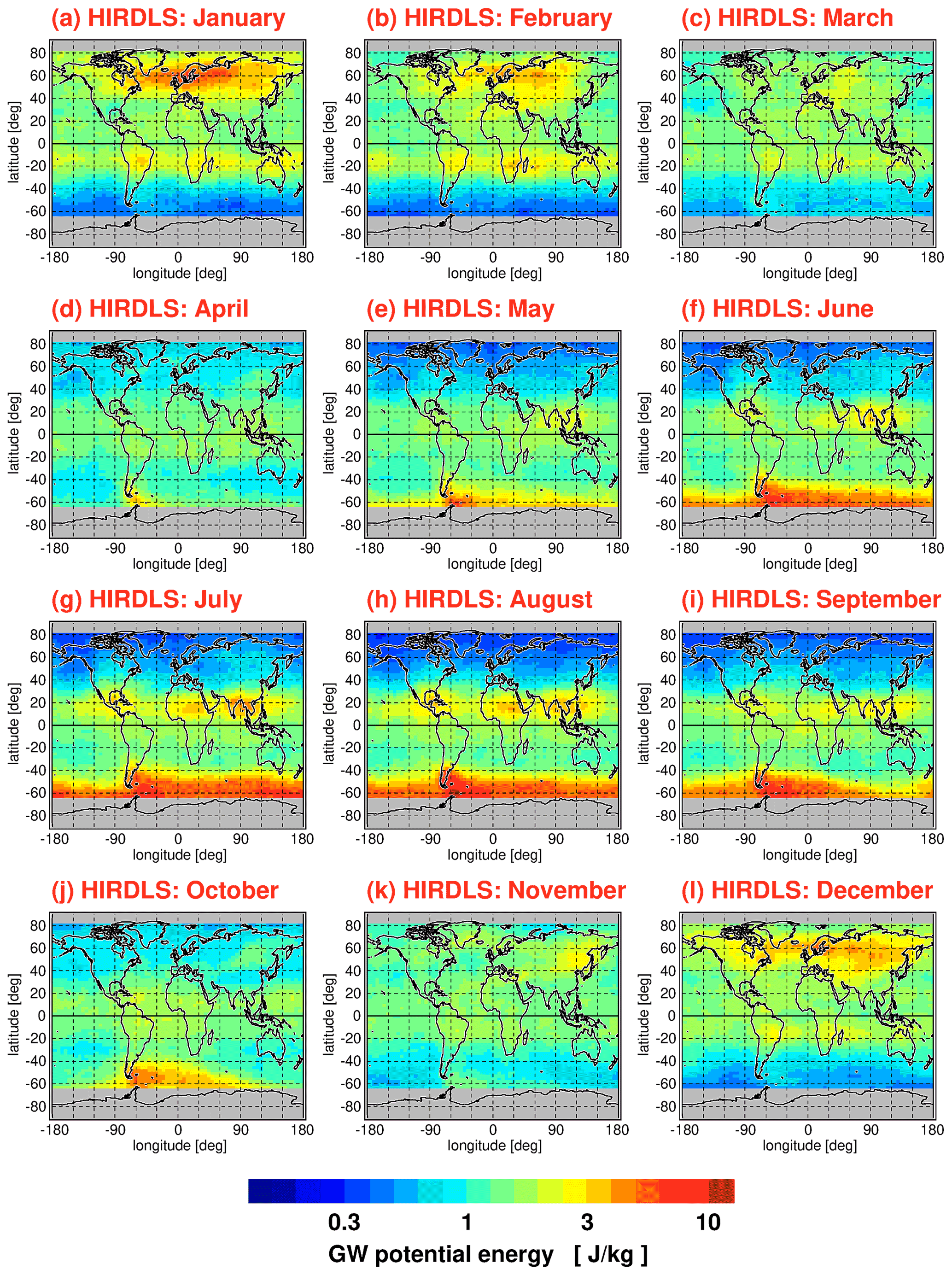
Figure 1 Global distributions of HIRDLS gravity wave (GW) potential energies at 30 km altitude for each calendar month. Values shown are multiyear means of monthly median values determined in overlapping 5^∘ × 15^∘ (latitude × longitude) grid boxes. The period used for averaging is March 2005 until February 2008.

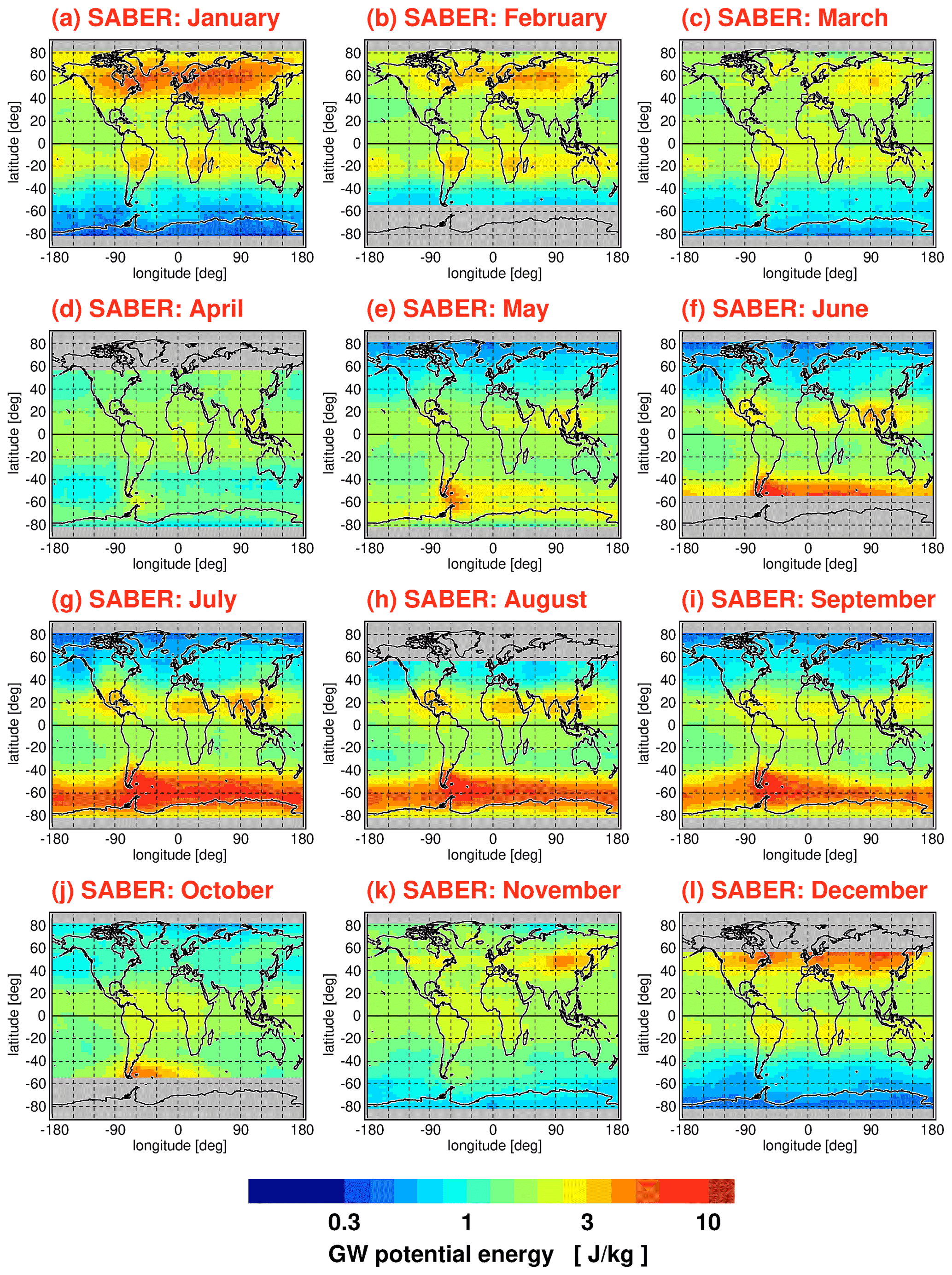
Figure 2 Global distributions of SABER gravity wave (GW) potential energies at 30 km altitude for each calendar month. Values shown are multiyear means of monthly median values determined in overlapping 10^∘ × 15^∘ (latitude × longitude) grid boxes. The period used for averaging is January 2002 to October 2020.

Similar to Figs. 1 and 2, Figs. 3 and 4 show global distributions of median absolute gravity wave momentum fluxes at 30 km altitude for each calendar month for HIRDLS (Fig. 3) and SABER (Fig. 4). For HIRDLS, we again use overlapping 5^∘ × 15^∘ (latitude × longitude) bins. For SABER, however, due to the reduced number of available data points, we use a coarser 20^∘ × 30^∘ resolution, i.e., worse than for SABER gravity wave potential energies. For this coarser resolution, we also use a coarser final grid of 5^∘ × 10^∘.

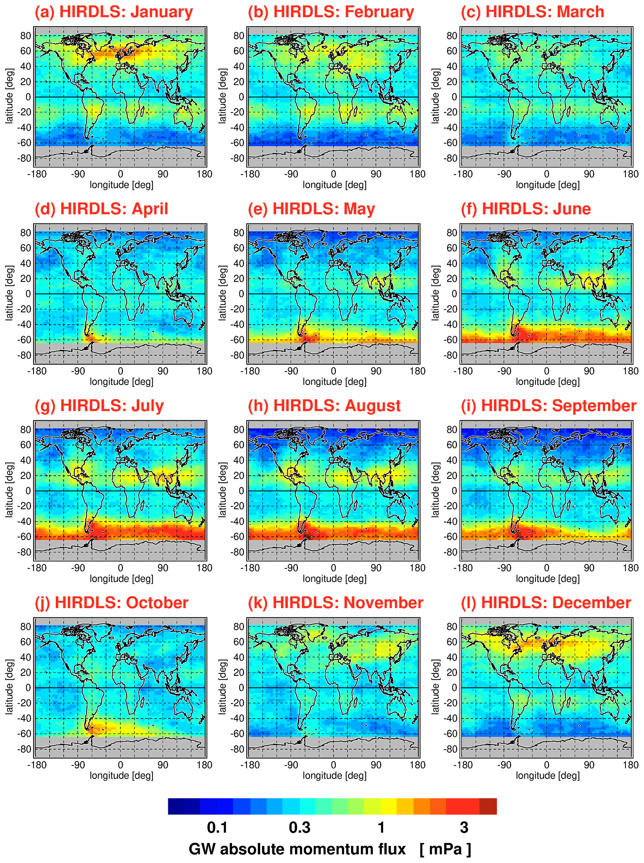
Figure 3 Same as Fig. 1 but for median HIRDLS gravity wave (GW) absolute momentum fluxes.

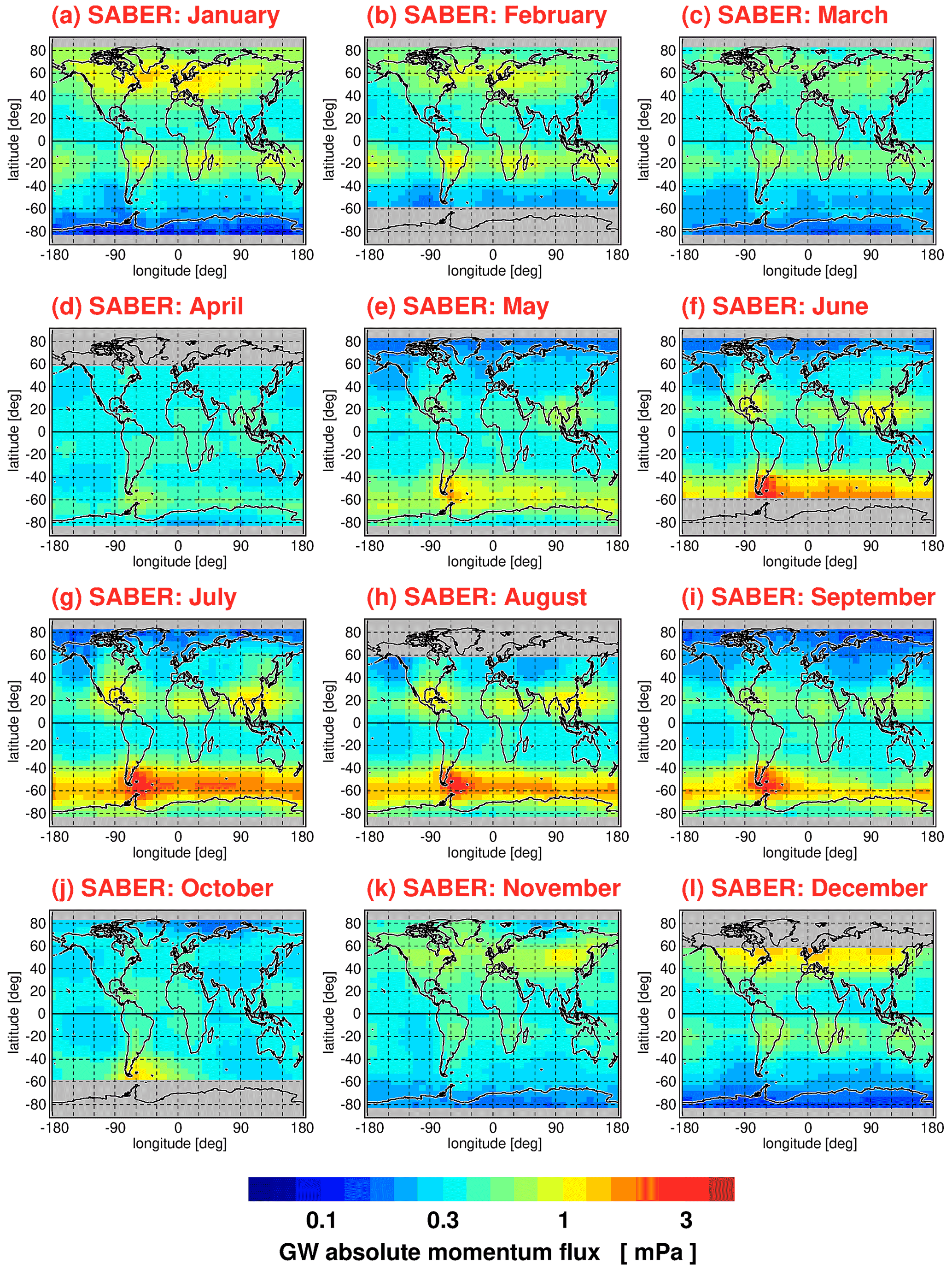
Figure 4 Same as Fig. 2 but for median SABER gravity wave (GW) absolute momentum fluxes determined in 20^∘ × 30^∘ (latitude × longitude) grid boxes.

The global distributions shown in Figs. 1–4 are the result of seasonally varying gravity wave sources and seasonally varying gravity wave propagation conditions given by the background winds and background temperature profile. In case of potential energies, seasonal variations in the background density are also important (for a discussion, the reader is referred to Strelnikova et al., 2021). In the subtropics of the respective summer hemisphere, characteristic enhancements of gravity wave activity are found that are likely caused by gravity waves excited by deep convection over the continents as well as over the Maritime Continent. At middle and high latitudes of the respective winter hemisphere, we find strong gravity wave activity in the polar night jets and their vicinity. Partly, these gravity waves are excited by jet-related source processes. Partly, mountain waves excited by flow over mountain ranges form hot spots, for example, over South America, the Antarctic Peninsula, Scandinavia, or Greenland. Overall, the global distributions of medians display relative variations that are very similar to the global distributions of arithmetic means shown in Ern et al. (2018).

4 Gravity wave intermittency investigated by probability density functions (PDFs)

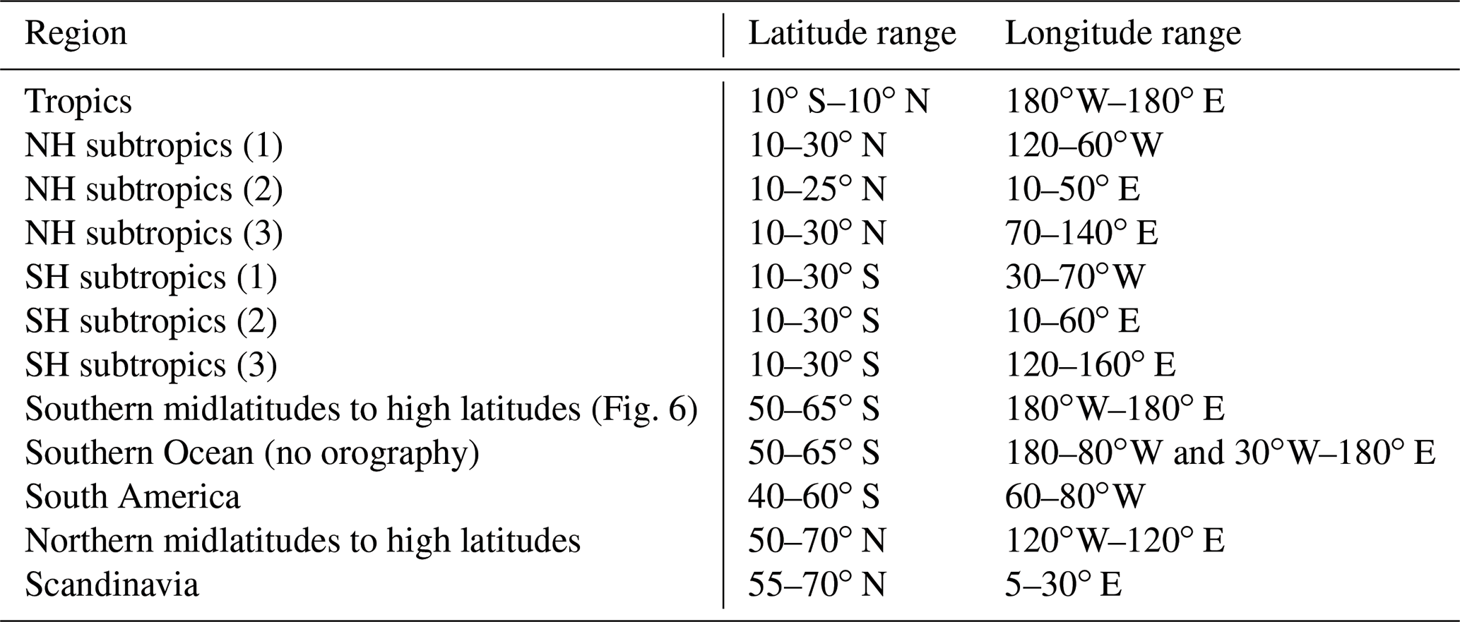
The global distributions in Figs. 1–4 show regular patterns that are similar in different years. In spite of these robust patterns, gravity wave activity is very intermittent, both spatially and temporally. Whenever intermittency of gravity wave distributions is determined, this requires collecting data temporally and/or spatially in a certain time interval or region. In our case, we collect data over 1 month in several predefined latitude–longitude intervals for a given altitude. Of course, these choices will have effect on the level of intermittency that is obtained in our analysis, as both temporal variations in gravity wave sources and of gravity wave propagation conditions within these intervals will contribute. The latitude–longitude regions selected in our work for determining PDFs are illustrated in Fig. 5, and the corresponding latitude and longitude ranges are summarized in Table 1.

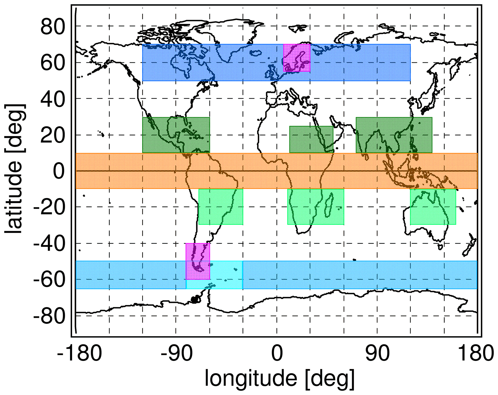
Figure 5 Illustration of the different regions selected for creating PDFs. The latitude–longitude ranges of the different regions are summarized in Table 1.

Table 1 Latitude–longitude ranges of the different regions illustrated in Fig. 5.

4.1 A first example: PDFs at Southern Hemisphere midlatitudes to high latitudes in October

One method to investigate the intermittency of the gravity wave distribution is the use of probability density functions (PDFs). As an example, for the latitude range 50–65^∘ S and all longitudes, Fig. 6a displays the absolute momentum flux PDF for the HIRDLS instrument at 30 km altitude for October 2005 (blue), October 2006 (red), and October 2007 (green), respectively. For all PDFs shown in Fig. 6, the mean, the 90th percentile, and the 99th percentile as well as the fractions of the mean momentum fluxes at values beyond the respective percentiles are given in Table 2.

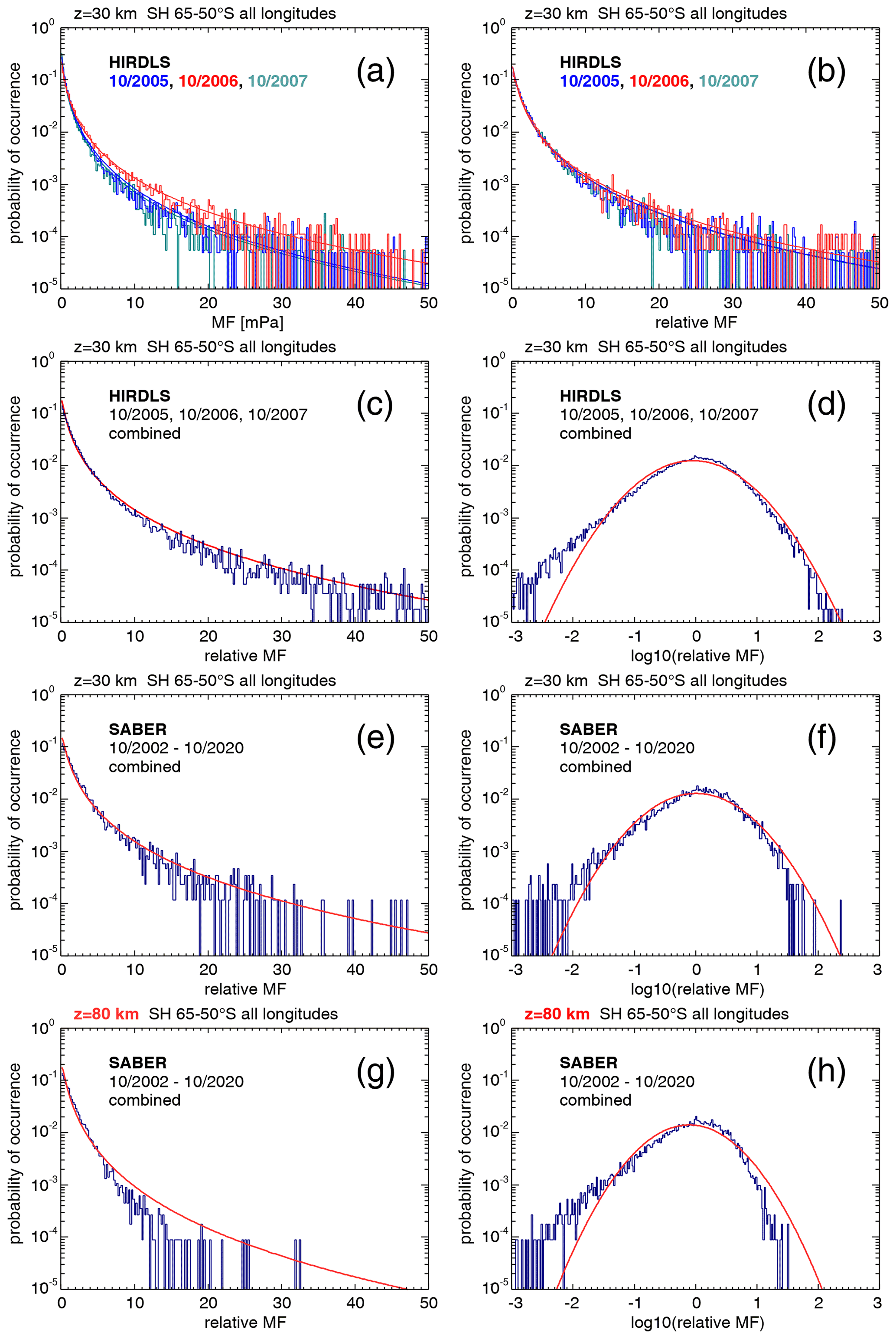
Figure 6 Probability density functions (PDFs) of (a) HIRDLS gravity wave absolute momentum fluxes (MF) over the Southern Ocean (latitudes 65–50^∘ S, all longitudes) at 30 km altitude for the month of October in the years 2005 (blue), 2006 (red), and 2007 (green). Panel (b) is the same as panel (a), but momentum fluxes were normalized by the monthly median global distribution. Panel (c) is the same as panel (b), but all years were combined into one PDF. Panel (d) is the same as panel (c) but on a logarithmic scale. Panel (e) is the same as panel (c) but for the SABER instrument and combining the October values for the years 2002–2020. Panel (f) is the same as panel (e) but on a logarithmic scale. Panel (g) is the same as panel (e) but for an altitude of 80 km. Panel (h) is the same as panel (g) but on a logarithmic scale. Red curves plotted in all panels are the corresponding lognormal distributions.

Table 2 Means, 90th percentiles, and 99th percentiles as well as fractions of gravity wave absolute momentum fluxes at values beyond the respective percentiles for the PDFs of momentum fluxes and normalized momentum fluxes shown in Fig. 6 for the month of October in the latitude band from 50 to 65^∘ S.

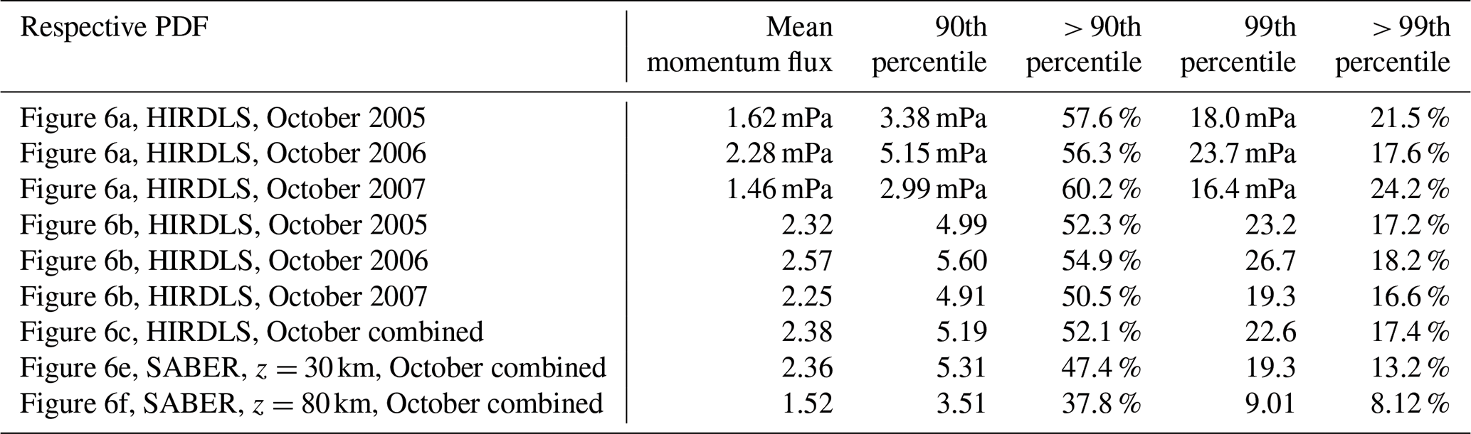
The region 50–65^∘ S is dominated by the Southern Ocean (flat terrain) except for South America (see also Fig. 5), which means that most gravity waves detected in this region are likely not mountain waves. Like in Hertzog et al. (2012), we find that the PDFs follow a lognormal distribution for each of the months. The respective lognormal distributions, which are characterized by the mean and the standard deviation of the logarithmic momentum flux values, are indicated by the smooth curves in the color of the respective year. The fact that the distributions are roughly lognormal means that the PDFs have a long tail at high momentum fluxes, and the largest 10 % (1 %) of values contribute as much as about 60 % (20 %) to the mean momentum flux in the region. This finding is similar to that for the HIRDLS data in Hertzog et al. (2012) (their Fig. 2).

It is, however, notable that the mean, median, and 90th percentile momentum fluxes in different years are different, whereas the shape of the PDFs is very similar. This means that if one wants to combine data from different years, the PDFs should be created by normalizing all values by, for example, the global distribution of median values. Further, it is shown in Appendix A that strong horizontal gradients of the global distribution can lead to spurious intermittency within a given region. The reason for this is that, by forming a PDF (or quantifying intermittency in another way), one assumes that all data points considered follow the same distribution with the same mean and the same standard deviation. This, however, is clearly not the case if there are horizontal gradients caused by variations in the overall global distribution within an area considered.

Therefore, in our study, we normalize values by the global distribution of spatially and temporally varying medians. For this, we determine the global distribution of medians, separately for each month in every year of available data, by applying the gridding based on latitude–longitude bins, as described in Sect. 3.2. We use the same bin sizes and the same latitude–longitude grids for the respective datasets as introduced in Sect. 3.2. The median of the respective latitude–longitude bin is attributed to the longitude and latitude of the bin center. For the normalization of a given momentum flux, or potential energy data point at a given altitude, we apply linear interpolation in longitude and time from the four surrounding bin centers to the latitude–longitude coordinate of the considered data point within an altitude profile. We do not apply temporal interpolation between different months and, instead, only use the global distribution of the month matching the time of the data point. In this way, we are able to better reduce the spurious intermittency due to horizontal gradients. However, we do not account for spurious intermittency that may arise from temporal variations in the global distribution on timescales shorter than about 1 month. (Please note that we do not use the distributions of the multiyear mean calendar months for normalization; instead, we use the distributions for the single months.)

Normalization by median values particularly makes sense if PDFs are expected to follow a lognormal distribution, as the median characterizes the center of a lognormal distribution. Normalization of distributions may be particularly important in the tropics and subtropics where the QBO modulates the gravity wave distribution, in addition to seasonal variations (e.g., Ern et al., 2011; Ern et al., 2014; Chen et al., 2019). Normalization of the PDFs also makes sense if only the shapes of the PDFs of different datasets are to be compared, but magnitudes are different. In the case of observations, this could happen if instruments have different observational filters for observing gravity waves. In the case of model data, differences in magnitude could arise from different model resolutions or from different model setups. Using normalization, it is even possible to compare completely different physical parameters that have different physical units.

Figure 6b shows the same as Fig. 6a, but the single momentum flux observations were normalized by the October global distribution of medians of the respective year. As can be seen from Fig. 6b, the PDFs of the different years are almost on top of each other, further demonstrating that the statistical properties of the momentum flux distributions in different years are very similar. Moreover, the relative contributions of momentum fluxes at values beyond the 99th percentiles are more similar for the normalized momentum fluxes (see Table 2). Further, the relative contributions of momentum fluxes at values beyond the respective percentiles are usually somewhat lower than those for the unnormalized momentum fluxes, indicating that local variations in momentum fluxes cause an overestimation of the intermittency of the PDFs when the unnormalized values are used. This again shows the advantage of using normalized values for PDFs.

It should also be noted that, in Hertzog et al. (2008), the ratio of the median (i.e., the 50th percentile) and the 90th percentile was introduced as a measure of intermittency. As the median of “normalized” PDFs is very close to unity, the 90th percentile of a normalized PDF can be directly taken as a measure of intermittency: the higher the 90th percentile of a normalized PDF, the stronger the intermittency of the distribution. This is a very practical application of using normalized values for creating PDFs. In particular, the 90th percentiles of normalized PDFs of different parameters, and thus the intermittency of the different parameters (for example, gravity wave potential energies and absolute momentum fluxes), can be directly compared. Because we are using local medians for normalization, not the overall median of all data points used for a PDF, it is not expected that the overall median of a normalized PDF is exactly unity.

As the distributions in different years are very similar, we combine the normalized gravity wave momentum flux values of the three PDFs into a single PDF. The result is shown in Fig. 6c. Again, the red curve represents the corresponding lognormal distribution. As can be seen from Table 2, the mean, the 90th and 99th percentiles, and the momentum flux relative contributions beyond the respective percentiles are close to the values of the single years.

Most previous studies displayed PDFs only on a linear scale, which made it difficult to investigate the shape of the PDF at low momentum flux values. To overcome this shortcoming, we also display (in Fig. 6d) the PDF of Fig. 6c on a logarithmic scale. As can be seen from Fig. 6d, the PDF also follows a lognormal distribution for a large range of 1–2 magnitudes of normalized momentum fluxes at values below zero (i.e., at values lower than the location of the distribution maximum). The PDF only starts to exceed the lognormal distribution at the very lowest values. As will be shown later in Sect. 4.2.4, measurement noise only partly affects the PDFs at low values of normalized momentum fluxes. The meaningful range of the PDFs for normalized momentum fluxes starts from about − 2 in most cases.

Figure 6e and f show the same as Fig. 6c and d but for the SABER instrument and combining the October data of the years 2002 until 2020. Obviously, the SABER PDFs in Fig. 6e and f are very similar to those of the HIRDLS instrument. The SABER PDFs only decrease more strongly than the HIRDLS PDFs at the very highest momentum fluxes. The likely reason for this is the coarser along-track sampling resolution of SABER (about twice the along-track sampling step of HIRDLS), which leads to stronger aliasing and stronger overestimation of the horizontal wavelength (i.e., underestimation of absolute momentum fluxes) of short horizontal wavelength gravity waves that potentially carry large momentum fluxes. This is also reflected in the reduced numbers of the 99th percentile and the momentum flux relative contribution beyond this percentile (given in Table 2).

Figure 6g and h show the same as Fig. 6e and f but for an altitude of 80 km. Compared with 30 km altitude, the distribution at 80 km is more strongly skewed toward low values. This is expected for two reasons. Firstly, the along-track sampling distance of those pairs of SABER altitude profiles that are used for calculating momentum fluxes increases with altitude, leading to stronger undersampling (aliasing) of gravity wave horizontal wavelengths and, thus, to low biases of gravity wave momentum fluxes (see Ern et al., 2011). Secondly, large-amplitude gravity waves that potentially carry stronger momentum fluxes will reach saturation at lower altitudes, dissipate, and are thus removed from the PDF. This also leads to much reduced numbers of the 90th and 99th percentiles as well as to reduced relative contributions of the momentum fluxes beyond the respective percentiles (see Table 2).

4.2 PDFs of gravity wave absolute momentum fluxes and potential energies for specific regions

In the following, we will investigate the characteristics of the PDFs in the different regions illustrated in Fig. 5. We focus on the HIRDLS instrument because of the better HIRDLS along-track sampling distance. Similar to Fig. 6c and d, we again combine the momentum fluxes of all years available for HIRDLS to improve statistics.

4.2.1 Gravity wave momentum flux PDFs in the tropics and in the respective summer hemisphere

Figure 7 shows PDFs of HIRDLS gravity wave absolute momentum fluxes at 30 km altitude in different regions in the tropics and the respective summer hemisphere. Figure 7a–c shows PDFs for the tropics in the latitude band 10^∘ S–10^∘ N and all HIRDLS observations from January 2005 until February 2008. The figure presents the PDFs for unnormalized momentum fluxes on a linear scale (Fig. 7a), the PDFs of momentum fluxes normalized by the monthly varying global distributions of medians (also on a linear scale) (Fig. 7b), and the PDFs of momentum fluxes normalized by the monthly varying global distributions of medians on a logarithmic scale (Fig. 7c). The mean, the 90th and 99th percentiles, and the fractions of the mean momentum fluxes at values beyond the respective percentiles for the different PDFs in Fig. 7 are given in Table 3.

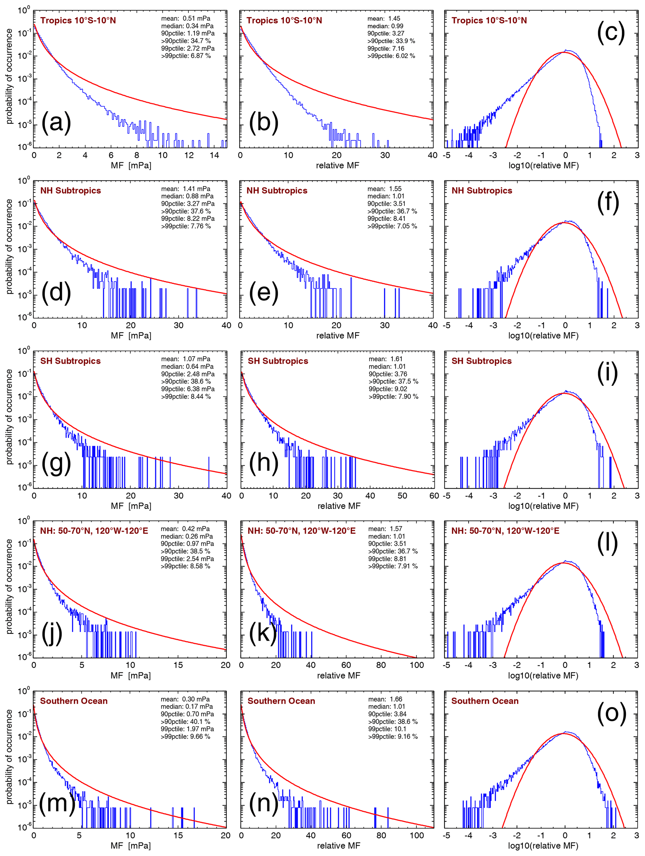
Figure 7 PDFs of HIRDLS gravity wave absolute momentum fluxes (MF) at 30 km altitude in the tropics for the period from January 2005 until February 2008 (a–c), for the three hot spots of gravity wave activity in the subtropics of the Northern Hemisphere during boreal summer (JJA) (d–f), for the three hot spots of gravity wave activity in the subtropics of the Southern Hemisphere during austral summer (DJF) (g–i), for the Northern Hemisphere midlatitude–high-latitude region from 50 to 70^∘ N and from 120^∘W to 120^∘ E during boreal summer (JJA) (j–l), and for the Southern Ocean region from 50^∘ S to 65^∘ N without the longitudes from 80 to 30^∘W during austral summer (DJF) (m–o). For an illustration of the locations of the different regions, see Fig. 5. Panels (a), (d), (g), (j), and (m) show gravity wave absolute momentum flux in millipascals (mPa), whereas the remaining panels show relative momentum flux.

Table 3 Means, 90th percentiles, and 99th percentiles as well as fractions of gravity wave absolute momentum fluxes at values beyond the respective percentiles for the PDFs of momentum fluxes (upper part of the table) and normalized momentum fluxes (lower part of the table) shown in Figs. 7 and 8.

Generally, the shapes of the unnormalized PDFs are quite similar to the PDFs composed of normalized momentum fluxes (and potential energies; see Sect. 4.2.3 below). The intermittency of unnormalized momentum fluxes is only generally somewhat stronger, as can be seen from the percentages of momentum fluxes beyond the 90th and 99th percentiles. However, the unnormalized PDFs and values in the different regions are not directly comparable in terms of their absolute values. Therefore, the following discussion will focus on the PDFs based on normalized values.

From the PDFs shown in Fig. 7a–c, it is evident that in the tropics the tail of the PDFs at large momentum fluxes is far below the red curve that represents a lognormal distribution, and the PDF is skewed toward low momentum flux values. Together with the somewhat reduced width of the fitted lognormal distribution in the tropics, this means that the distribution of gravity wave momentum fluxes in the tropics is much less intermittent than the distribution at high latitudes during winter (see Fig. 6). This is in agreement with previous findings by Wright et al. (2013) and Ern et al. (2014) for HIRDLS momentum fluxes. Moreover, the percentages of momentum fluxes beyond the 90th percentiles are in good agreement with previous findings in the tropics (Wright et al., 2013; Ern et al., 2014; Corcos et al., 2021). (Please note that, in contrast to Jewtoukoff et al., 2013, Corcos et al., 2021 did not use superpressure balloon observations above nighttime clouds that lead to high-biased momentum fluxes and possibly to overly long tails at high momentum fluxes in tropical gravity wave momentum flux PDFs.)

Figure 7d–i show the PDFs for the gravity wave hot spot regions in the summertime subtropics (see Figs. 1–4) that were previously discussed by Ern and Preusse (2012). Even in these regions of enhanced gravity wave activity during the summer months, the characteristics of the PDFs are similar to in the tropics; intermittency is only somewhat enhanced compared to the tropics, as can be seen from the 90th and 99th percentiles of the normalized PDFs given in Table 3.

Furthermore, the PDFs shown in Fig. 7j–o, which represent midlatitude and high-latitude regions in the respective summer hemisphere, are skewed towards low values. The normalized PDFs are very similar to those in the summertime subtropics, and intermittency is also similar to that for the distributions in the summertime subtropics (see the similar 90th and 99th percentiles for the normalized PDFs given in Table 3).

In the tropics and summertime subtropics, it is expected that deep convection is one of the main gravity wave source processes (e.g., Beres et al., 2004; Song and Chun, 2005; Kang et al., 2017, 2018). Infrared limb sounding satellite instruments can only observe gravity waves with horizontal wavelengths longer than 100–200 km (intrinsic periods longer than 1–2 h; see Alexander et al., 2010). These long horizontal wavelengths are attributable rather to mesoscale convective systems than to single convective cells that usually excite gravity waves of shorter horizontal scales and shorter intrinsic periods (e.g., Trinh et al., 2016). Therefore, it should be pointed out that our work focuses only on the part of the gravity wave spectrum seen by infrared limb sounders, and the intermittency of gravity waves can be different in different parts of the gravity wave spectrum. In particular, superpressure balloon observations indicate that convective gravity waves of intrinsic periods shorter than 1 h are more intermittent than convective gravity waves of longer intrinsic periods (Corcos et al., 2021).

4.2.2 Gravity wave momentum flux PDFs in the respective winter hemisphere

Figure 8 shows PDFs of HIRDLS gravity wave absolute momentum fluxes at 30 km altitude for middle and high latitudes in the respective winter hemisphere. Figure 8a–c show PDFs for gravity wave momentum fluxes in the austral winter season from June until August over the Southern Ocean (i.e., the latitude band 50–65^∘ S without the longitude range 30–80^∘ W). By omitting the longitude range 30–80^∘ W, the gravity wave hot spot over South America is excluded that is likely dominated by mountain waves. In this way, we focus on the intermittency of non-orographic gravity waves over the Southern Ocean. Compared to the situation in October shown in Fig. 6, the PDFs over the Southern Ocean (shown in Fig. 8a–c) are very similar, but they decrease somewhat more strongly than lognormality at high values. Likely reason is that the very high gravity wave momentum fluxes of the hot spot over South America are not included in the PDFs shown in Fig. 8a–c. As can be seen from Tables 2 and 3, the 90th and 99th percentiles for normalized momentum fluxes during June to August are very similar to the percentiles of the corresponding distributions shown in Fig. 6, whereas the momentum flux fraction at values beyond the 99th percentile is somewhat higher for Fig. 6.

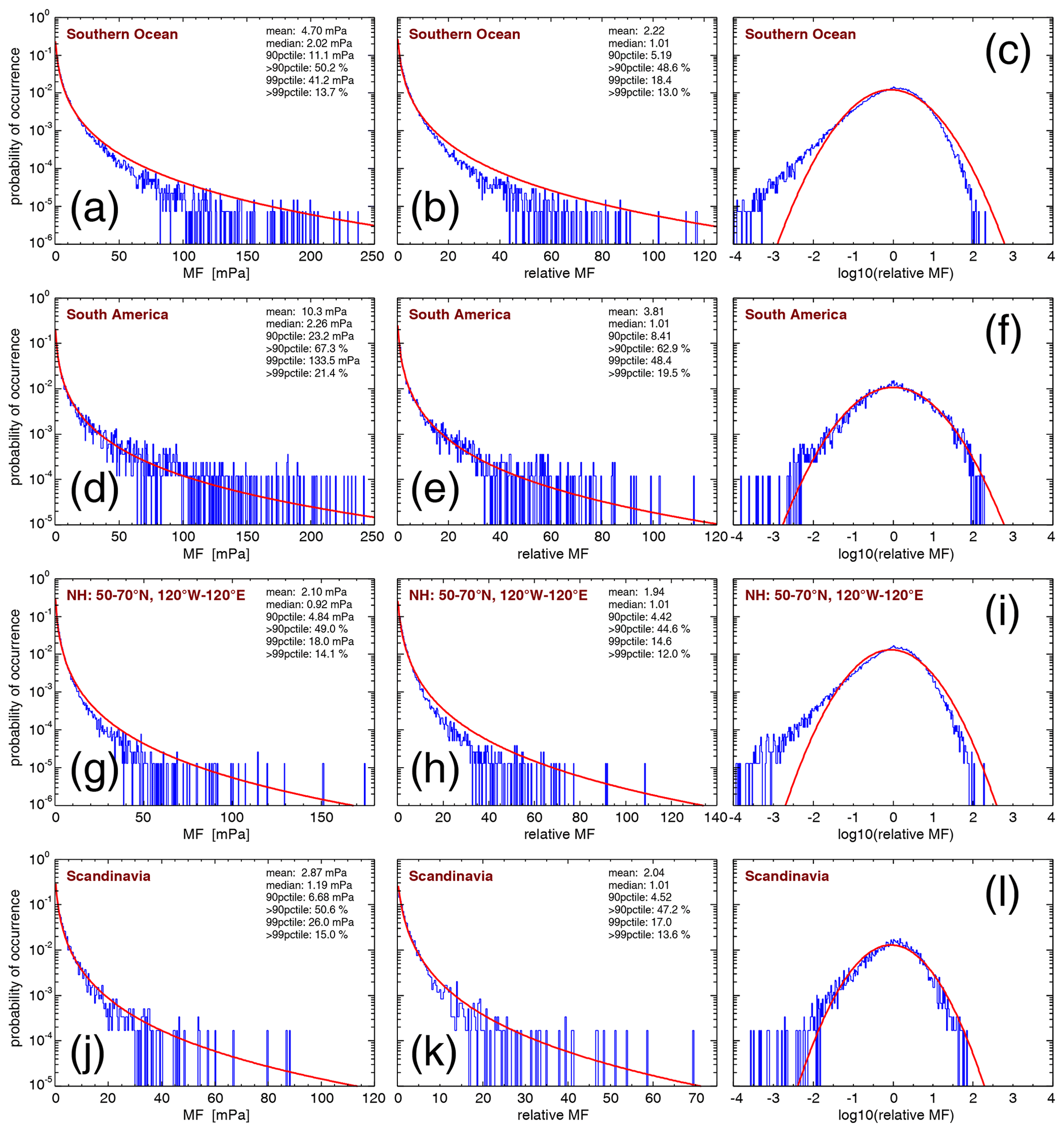
Figure 8 PDFs of HIRDLS gravity wave absolute momentum fluxes (MF) at 30 km altitude for the Southern Ocean during austral winter (JJA) (a–c), for the region of the gravity wave hot spot over South America during austral winter (JJA) (d–f), for the region of enhanced gravity wave activity in the Northern Hemisphere polar night jet during boreal winter (DJF) (g–i), and for Scandinavia and its close vicinity during boreal winter (DJF) (j–l). For an illustration of the locations of the different regions, see Fig. 5. Panels (a), (d), (g), and (j) show gravity wave absolute momentum flux in millipascals (mPa), whereas the remaining panels show relative momentum flux.

Because the likely reason for the abovementioned differences are the orographic gravity waves over South America, we will next investigate the PDFs of the gravity wave hot spot over South America. Figure 8d–f show PDFs for gravity wave momentum fluxes in the austral winter season from June until August in the region from 40 to 60^∘ S and from 60 to 80^∘W (i.e., the region of the gravity wave hot spot over South America that is likely dominated by mountain waves). As has been stated before by, for example, Hertzog et al. (2008), Hertzog et al. (2012), and Wright et al. (2013), gravity waves excited by orographic sources are very intermittent. This is the case because this source mechanism depends on the strongly variable near-surface winds. As can be seen from Fig. 8e, the PDF indeed exceeds a lognormal distribution at relative momentum fluxes in the range of about 10–30. Moreover, the 90th and 99th percentiles of the relative momentum fluxes over South America are the highest values to be found in Table 3. However, the PDF does not exceed the lognormal distribution as strongly as has been found for the momentum fluxes observed by superpressure balloons or those simulated by high-resolution models (e.g., Hertzog et al., 2008, 2012). At relative momentum fluxes above 30, the PDFs in Fig. 8e and f even drop below the lognormal distribution. This is likely an effect of the observational filter that applies for limb sounding satellite instruments. The very highest momentum fluxes are likely carried by gravity waves of quite short horizontal wavelength. However, horizontal wavelengths shorter than about 100 km cannot be seen by HIRDLS and SABER. In addition, short horizontal wavelengths that are still seen by HIRDLS and SABER will suffer from amplitude low biases by the sensitivity function of limb sounders (e.g., Preusse et al., 2002; Ern et al., 2018, and references therein) as well as an undersampling and, thus, overestimation of horizontal wavelengths, resulting in low-biased momentum fluxes.

It is also noteworthy that gravity wave observations by the Atmospheric Infrared Sounder (AIRS) show similar characteristics at middle and high southern latitudes (Hindley et al., 2019). Although AIRS has a very different observational filter and observes only gravity waves with a vertical wavelength longer than about 12 km (e.g., Ern et al., 2017; Meyer et al., 2018), very strong intermittency is found over South America and the Antarctic Peninsula, and somewhat weaker, although still strong, intermittency is found over the Southern Ocean.

In order to find out whether there are hemispheric differences, we will investigate PDFs of the gravity waves in the Northern Hemisphere at middle and high latitudes during boreal winter. Figure 8g–i show PDFs for gravity wave momentum fluxes in the boreal winter season December until February in the region from 50 to 70^∘ N and from 120^∘W to 120^∘ E, which corresponds to enhanced values of gravity wave activity related to the Northern Hemisphere polar night jet (see also Figs. 1–4). Obviously, the PDFs of normalized momentum fluxes in Fig. 8h and i are very similar to those over the Southern Ocean (Fig. 8b, c). The 90th and 99th percentiles of normalized momentum fluxes, however, are somewhat lower than over the Southern Ocean, which indicates that the gravity wave distribution in the Northern Hemisphere polar night jet region is less intermittent on average.

Hot spots of gravity wave activity in the Northern Hemisphere during boreal winter that are linked to orography are usually less pronounced than the gravity wave hot spot over South America during austral winter (see Figs. 1–4). One of the reasons might be that, due to the more pronounced large-scale orography, Rossby wave activity in the Northern Hemisphere is usually stronger. Therefore, it is expected that jet-related gravity wave source processes act more continuously, and hot spots of mountain wave activity are therefore swamped with gravity waves from other sources. Given the strong activity of jet-related gravity waves sources, it may appear counterintuitive that gravity wave amplitudes in the Northern Hemisphere during boreal winter are much lower than in the Southern Hemisphere during austral winter. However, during the respective winter season, background winds are usually much weaker in the Northern Hemisphere than in the Southern Hemisphere. This makes gravity wave propagation conditions less favorable in the Northern Hemisphere during boreal winter and limits the maximum amplitudes that gravity waves can attain. Therefore jet-related gravity wave source processes could still act more continuously. Another effect that can lead to less pronounced hot spots of mountain wave activity in the Northern Hemisphere is that mountain waves can be advected over large distances and, in the stratosphere, do not necessarily occur over the mountain range where they were excited (e.g., Krisch et al., 2017).

Still, mountain waves are often observed near their sources, for example over Scandinavia (e.g., Doernbrack and Leutbecher, 2001; Gisinger et al., 2020). Therefore, in order to also include a region in the Northern Hemisphere where mountain waves are repeatedly observed, Fig. 8j–l show PDFs for gravity wave momentum fluxes in the boreal winter season from December until February in the region from 55 to 70^∘ N and from 5 to 30^∘ E, which roughly corresponds to Scandinavia and its close vicinity.

Indeed, for relative momentum fluxes in the range from 10 to 20, the PDFs shown in Fig. 8k and l are somewhat closer to a lognormal distribution than those shown in Fig. 8h and i. Further, the PDF in Fig. 8l has a less pronounced tail at low values of relative momentum fluxes than the PDF in Fig. 8i. However, at high values of relative momentum fluxes, the PDFs in Fig. 8k and l do not show an enhancement as strong as seen in the South America region (see Fig. 8e and f). This means that the PDFs over Scandinavia are an intermediate state between those PDFs dominated by non-orographic gravity wave sources (Southern Ocean and Northern Hemisphere polar night jet regions) and PDFs that are more strongly dominated by orographic sources (South American region). This might indicate that a mixture of mountain waves and non-orographic waves is often observed over Scandinavia. Indeed, several case studies show that non-orographic gravity waves are frequently seen over Scandinavia (e.g., Réchou et al., 2013; Krisch et al., 2020).

4.2.3 PDFs of gravity wave potential energies

In addition to gravity wave momentum fluxes, gravity wave potential energies are also of interest for comparison with other instruments or with model data. Therefore, Figs. 9 and 10 show PDFs for the same regions as in Figs. 7 and 8 but for gravity wave potential energies. Similar to Table 3, Table 4 shows the 90th and 99th percentiles of the PDFs as well as the corresponding fractions of potential energies at values beyond the respective percentiles.

Figure 9 Same as Fig. 7 but for gravity wave potential energies (E_pot).

Figure 10 Same as Fig. 8 but for gravity wave potential energies (E_pot).

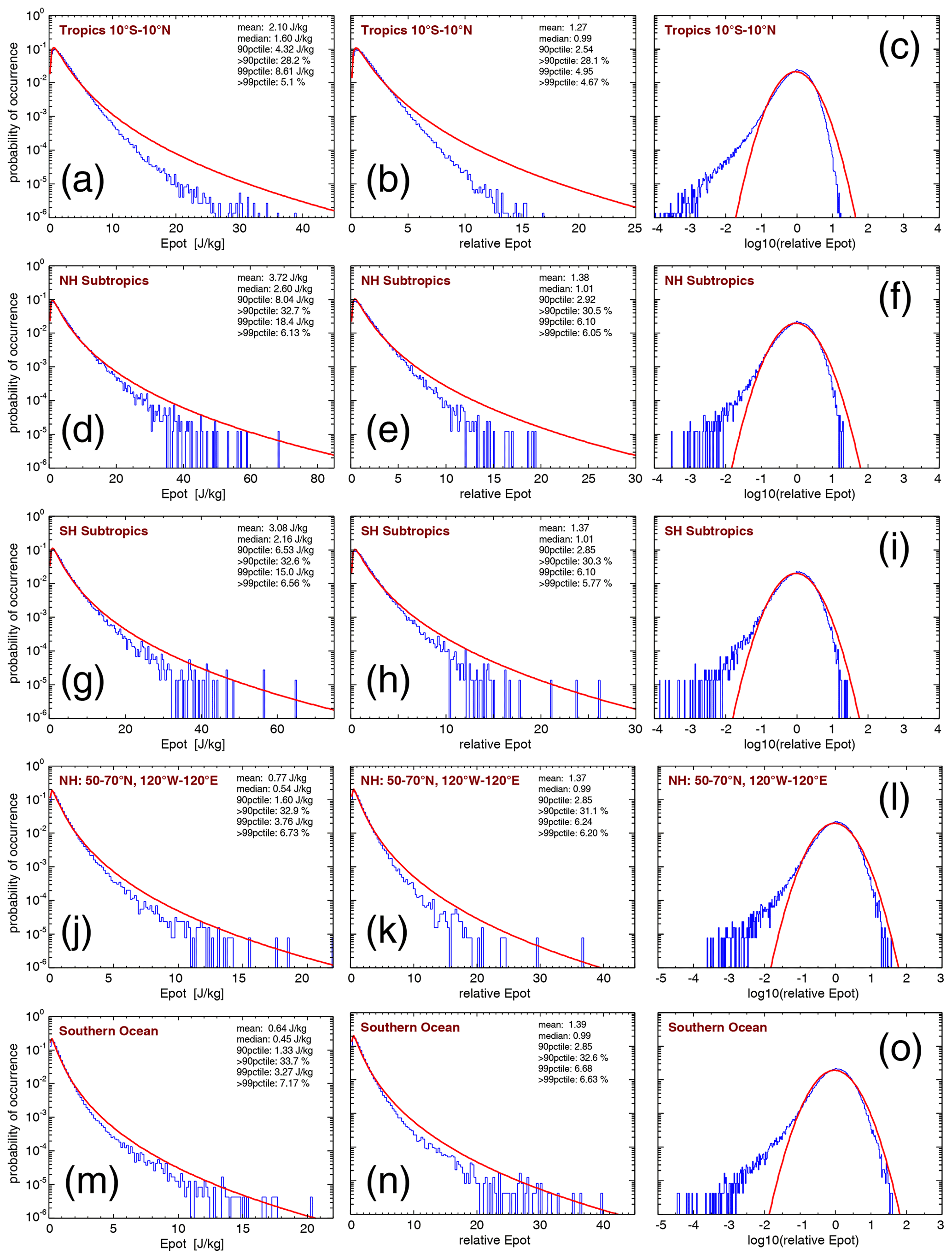
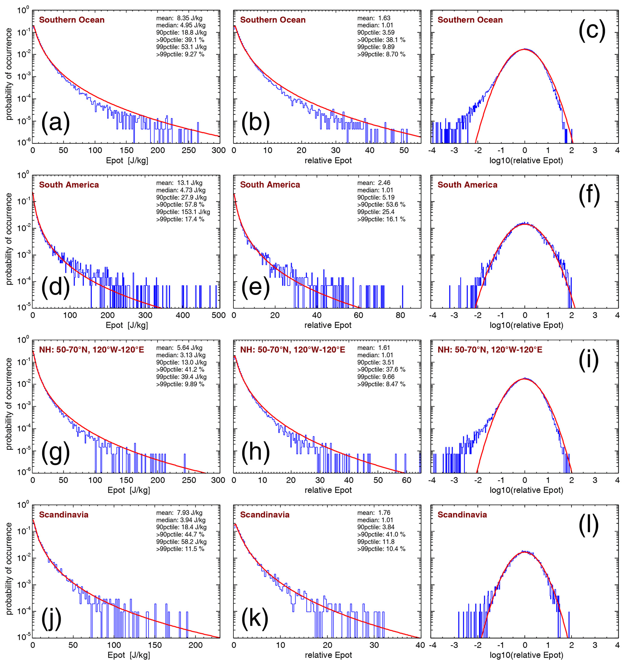
Table 4 Means, 90th percentiles, and 99th percentiles as well as fractions of gravity wave potential energies at values beyond the respective percentiles for the PDFs of potential energies (upper part of the table) and normalized potential energies (lower part of the table) shown in Figs. 9 and 10.

Similar to the PDFs for gravity wave absolute momentum fluxes, the PDFs for gravity wave potential energies roughly follow lognormal distributions. This has been pointed out before by, for example, Baumgaertner and McDonald (2007). As is evident from Figs. 7–10, the shapes of the potential energy PDFs in the different regions are very similar to the shapes of the corresponding momentum flux PDFs. This is noteworthy, as one might expect that the shape of the momentum flux PDFs could be skewed by biases introduced by the satellite sampling and the corresponding biases in horizontal wavelength estimates. Obviously, however, these biases have no strong effect on the overall shape of the PDFs.

The main difference between potential energy PDFs and momentum flux PDFs is that the potential energy PDFs are generally narrower than the corresponding momentum flux PDFs. This is also reflected in the lower numbers of 90th and 99th percentiles of relative potential energy PDFs, compared with PDFs for relative momentum fluxes. The same holds for the fractions of relative momentum fluxes and relative potential energies at values beyond the respective percentiles. The reduced numbers for potential energy PDFs indicate that potential energy distributions are less intermittent than absolute momentum flux distributions. This finding is as expected because gravity wave horizontal and vertical wavelengths also enter into the calculation of momentum fluxes. These additional parameters will add further variability; thus, they contribute to the stronger intermittency of momentum fluxes compared with potential energies.

4.2.4 The effect of measurement noise

The intermittency of gravity wave potential energies is almost exclusively introduced by the intermittency of gravity wave squared temperature amplitudes (see Eq. 5). This allows us to investigate the reliability of the long tails of PDFs at low potential energies (and momentum fluxes). Generally, measurement noise should result in a high bias of squared temperature amplitudes (and, thus, potential energies) of weak gravity wave events.

As an example, we will now roughly estimate the extent to which the parts of PDFs at low values may be affected by measurement noise. At 30 km altitude, the precision σ of temperature observations is about σ=0.4 K for HIRDLS and σ=0.3 K for SABER (e.g., Gille et al., 2011; Ern et al., 2018, and references therein). In our study, we determine temperature amplitudes $\widehat{T}$ in sliding vertical windows of 10 km extent. According to the respective vertical field of view, n=10 (n=5) independent values enter an amplitude estimate for HIRDLS (SABER), which reduces the noise-induced uncertainty by the averaging effect. The corresponding noise-equivalent temperature amplitude is ${\widehat{T}}_{\mathrm{noise}}=\mathit{\sigma }/\sqrt{n}$ (i.e., about 0.13 K for both HIRDLS and SABER). According to Eq. (5), we can calculate the noise-equivalent gravity wave potential energy:

$$\begin{array}{}\text{(8)}& E_{\mathrm{pot},\mathrm{noise}}={\displaystyle \frac{\mathrm{1}}{\mathrm{4}}}{\left({\displaystyle \frac{g}{N}}\right)}^{\mathrm{2}}{\left({\displaystyle \frac{{\widehat{T}}_{\mathrm{noise}}}{\stackrel{\mathrm{‾}}{T}}}\right)}^{\mathrm{2}}.\end{array}$$

Inserting typical values for the lower stratosphere of g=9.8 m s⁻², $\stackrel{\mathrm{‾}}{T}=\mathrm{230}$ K, N=0.02 s⁻¹, and ${\widehat{T}}_{\mathrm{noise}}=\mathrm{0.13}$ K, we obtain $E_{\mathrm{pot},\mathrm{noise}}\approx \mathrm{0.02}$ J kg⁻¹ for HIRDLS and SABER at altitudes around 30 km. Dividing this value by the respective medians given in panels a, d, g, and j in Figs. 9 and 10 and taking the base-10 logarithm, we obtain values between about −1.9 and −2.4 for all regions, except for midlatitude and high-latitude regions in the respective summer hemisphere (for which we obtain values of around −1). This means that in all PDFs shown in panels c, f, i, and l of Figs. 9 and 10, the peaks of the distribution as well as a large part of the tails of the distributions at low relative gravity wave potential energies are well resolved. It can be assumed that this finding also holds for the PDFs of gravity wave absolute momentum fluxes, and similar considerations can be made also for other altitudes.

5 Gravity wave intermittency investigated by the Gini coefficient

5.1 The Gini coefficient

While PDFs give comprehensive information on intermittency in a given time interval and region, it takes a large number of observations to create a robust PDF. This comes at the cost of losing spatial and temporal resolution and, potentially, combining different regions of different intermittency into one PDF. In such cases, even the use of normalized values for creating a PDF does not help. Further, PDFs do not provide an integral number that allows one to display the distribution of intermittency in global maps.

One way to overcome these limitations is the introduction of intermittency coefficients. For gravity wave absolute momentum fluxes observed by superpressure balloons, Hertzog et al. (2008) introduced the Bernoulli coefficient and the 90th-percentile coefficient. Later, however, Plougonven et al. (2013) found that another coefficient – the Gini coefficient (Gini, 1912) – is preferable for high-resolution model simulations. Therefore, in the following, we will also use the Gini coefficient for displaying intermittency distributions. To calculate the Gini coefficient, the dataset consisting of N observations f_i is first sorted, such that $\mathrm{1}\le i\le N$ with $f_i\le f_{i+\mathrm{1}}$. After that, a set of cumulative sums F_n is calculated for $n=\mathrm{1},\mathrm{\dots },N-\mathrm{1}$:

$$\begin{array}{}\text{(9)}& F_n=\sum _{i=\mathrm{1}}^n{f}_i.\end{array}$$

The Gini coefficient I_g is then defined as follows:

$$\begin{array}{}\text{(10)}& I_g={\displaystyle \frac{{\sum }_{n=\mathrm{1}}^{N-\mathrm{1}}\left(n\stackrel{\mathrm{‾}}{f}-F_n\right)}{{\sum }_{n=\mathrm{1}}^{N-\mathrm{1}}n\stackrel{\mathrm{‾}}{f}}},\end{array}$$

where $\stackrel{\mathrm{‾}}{f}$ is the arithmetic mean of the dataset.

Values of the Gini coefficient are between 0 and 1, and a higher Gini coefficient denotes stronger intermittency. The two extreme cases are (1) all values f_n are equal, and (2) all values are negligible (zero) except for one single value that dominates the arithmetic mean of the dataset. In case (1), intermittency is as low as possible, and I_g=0. In case (2), intermittency is as strong as possible, and I_g=1.

One problem, however, remains: because of the low number of available data points, relatively large latitude–longitude bins of 20^∘ × 30^∘ are required to determine global distributions of SABER absolute momentum fluxes. In the presence of strong spatial gradients of the global distribution, this will lead to biases of the global distribution of intermittency coefficients.

As can be seen from Eq. (10), the Gini coefficient is a relative measure and does not depend on the average magnitude of the dataset. This means that, in order to reduce the biassing effect of spatial gradients within given latitude–longitude bins, similar to the method used for PDFs, single values can be normalized by, for example, the monthly mean or median distribution. In regions of low gradients, the normalization of values will leave values of I_g unaltered, whereas the use of normalized values in regions of strong gradients will reduce the biases of I_g. Therefore, we apply the same procedure as for the normalized PDFs: before calculating the global distributions of I_g, we generally normalize the values of gravity wave potential energies or absolute momentum fluxes by the monthly global distribution of medians determined in the sets of latitude–longitude bins used in our study (see Sects. 3.2 and 4.1) and then interpolate to the location of each observation. This is performed separately for each month. It should be noted that global distributions of I_g would be almost unchanged if we would normalize by the monthly global distribution of mean values, instead of the monthly global distribution of medians. One possible reason for this similarity could be that, for every latitude–longitude bin used for calculating the global distributions of I_g, the median differs from the mean by a factor that does not vary much within a bin. If this is the case, the Gini coefficient for a bin would be almost the same for both kinds of normalization. Still, the factor between the mean and median could vary from bin to bin without having much effect on the global distribution of I_g.

For HIRDLS, global distributions of I_g are almost unchanged by this normalization procedure because relatively small 5^∘ × 15^∘ (latitude × longitude) bins are used for calculating global distributions. Obviously, the effect of spatial gradients within these small bins can be widely neglected. The same holds for global distributions of I_g for SABER potential energies that are based on 10^∘ × 15^∘ bins. However, for the SABER distributions of momentum fluxes that are calculated with a 20^∘ × 30^∘ bin size, values of I_g in regions of strong spatial gradients are strongly reduced if normalization is applied (see Sect. 5.2.2 and Appendix A), and the distributions become more similar to the corresponding HIRDLS distributions of I_g. The resulting HIRDLS and SABER global distributions of Gini coefficients at 30 km altitude (i.e., at a relatively low altitude) will be discussed in the following subsection (Sect. 5.2).

5.2 Global distributions of Gini coefficients

Distributions of Gini coefficients have previously been derived for gravity wave potential energies (e.g., Baumgaertner and McDonald, 2007) and for gravity wave absolute momentum fluxes (e.g., Hertzog et al., 2008, 2012; Wright et al., 2013). Based on gravity wave amplitudes, the calculation of potential energies from satellite observations can be performed for each individual altitude profile, whereas the calculation of momentum fluxes requires assumptions regarding how different altitude profiles can be combined. Particularly for SABER, the along-track sampling distance for 50 % of the observed altitude profiles is too large for momentum fluxes to be calculated. Further, for calculating momentum fluxes, a certain number of altitude profiles have to be discarded due to nonmatching vertical wavelengths (see also Ern et al., 2018, and references therein). Therefore, global distributions of Gini coefficients for gravity wave potential energies are based on a much better statistics, and we will discuss these distributions first.

5.2.1 Gini coefficients for gravity wave potential energies

Figure 11 shows global distributions of Gini coefficients for HIRDLS gravity wave potential energies at 30 km altitude. The different panels in Fig. 11 represent different average calendar months. Averaging over the the respective monthly distributions was performed for the period from March 2005 until February 2008 (i.e., 3 full years). For the global distributions, Gini coefficients were determined in overlapping bins of 5^∘ × 15^∘ (latitude × longitude), and only those bins that contained more than 40 data points were used. As discussed in Sect. 5.1, Gini coefficients were calculated from normalized potential energies, which means that each potential energy data point was normalized by the E_pot value of the corresponding monthly median E_pot distribution, interpolated to the exact location of each data point considered.

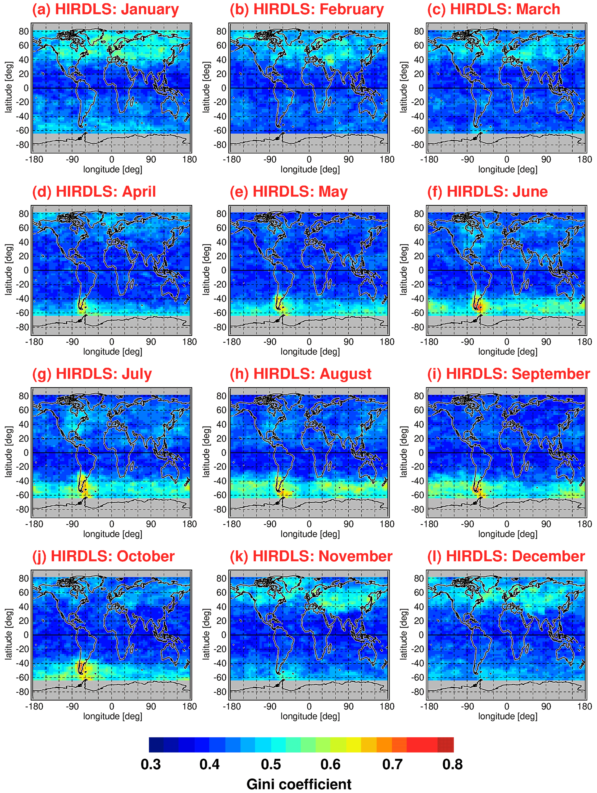
Figure 11 Global distributions of the Gini coefficients for HIRDLS gravity wave potential energies at 30 km altitude for each calendar month. Values shown are multiyear means of monthly values determined in overlapping 5^∘ × 15^∘ (latitude × longitude) grid boxes. Single E_pot values were normalized by the monthly median distribution before calculating the Gini coefficients. The period used for averaging is March 2005 to February 2008.

As can be seen from Fig. 11, the global distribution of Gini coefficients exhibits seasonal variations that are linked to seasonal variations in the potential energy distributions (see Fig. 1). Particularly high values of the Gini coefficient are found in the respective winter hemisphere at middle and high latitudes. In the winter season, these regions are dominated by the polar night jets. The gravity waves in these regions are mainly excited by flow over orography (mountain waves) and by jet-related source processes. The corresponding gravity wave sources are highly variable, as they depend on the strongly variable near-surface winds and on the strongly variable wind jets and weather systems, respectively. In addition, the strong winds in the polar night jets offer favorable propagation conditions for the gravity waves excited by these mechanisms.

In the months from April to October, the latitude range of about 40^∘–65^∘ S is dominated by the Southern Hemisphere polar night jet. During this period, maximum intermittency of I_g up to values of about 0.7 is found over the southern tip of South America and over the Antarctic Peninsula. These regions are well known as source regions of very strong and very intermittent mountain waves (e.g., Hertzog et al., 2008). In the same period and latitude range, intermittency over the Southern Ocean is still quite strong with values of I_g around 0.5.

Similarly, in the Northern Hemisphere, the latitude range of about 40^∘–65^∘ N is dominated by the Northern Hemisphere polar night jet during the months of November to February. Gini coefficients in the Northern Hemisphere polar night jet are about as strong as in the Southern Hemisphere polar night jet over the ocean. However, peak values as high as over the southern tip of South America and the Antarctic Peninsula are not attained.

At latitudes equatorward of about 30^∘ to 40^∘, Gini coefficients are comparably low (around 0.4). Still, there is a hemispheric asymmetry with somewhat higher values in the subtropics of the respective summer hemisphere. As can be seen in the global distributions of E_pot, there are enhancements in the summertime subtropics which are related to gravity waves that are excited by deep convection (e.g., Jiang et al., 2004; Wright and Gille, 2011; Ern and Preusse, 2012; Trinh et al., 2016; Kalisch et al., 2016; Stephan et al., 2019b). These gravity waves seem to be somewhat more intermittent than convectively generated gravity waves in the tropics, which confirms our results obtained for the PDFs in Sect. 4.2.1. Moreover, at midlatitudes in boreal summer over North America, intermittency is somewhat enhanced, which is possibly related to thunderstorms in the summer season that are known to excite strong gravity waves (e.g., Hoffmann and Alexander, 2010).

Figure 12 shows the same as Fig. 11 but for the SABER instrument. However, for SABER, Gini coefficients were calculated in overlapping bins of 10^∘ × 15^∘ (latitude × longitude) because of the lower number of data points per month available for SABER. The SABER number of data points per month is particularly low at high latitudes during months when the SABER viewing geometry (and thus the covered latitude range) changes. Another difference between Fig. 11 and Fig. 12 is that the distributions shown in Fig. 12 were obtained by averaging over a longer period (January 2002 until October 2020). The corresponding E_pot distributions are shown in Fig. 2.

Figure 12 Global distributions of the Gini coefficients for SABER gravity wave potential energies at 30 km altitude for each calendar month. Values shown are multiyear means of monthly values determined in overlapping 10^∘ × 15^∘ (latitude × longitude) grid boxes. Single E_pot values were normalized by the monthly median distribution before calculating the Gini coefficients. The period used for averaging is January 2002 to October 2020.

Obviously, the relative distributions of Gini coefficients in Figs. 11 and 12 are very similar, even though the spatial resolution of the SABER distributions is somewhat worse. On average, Gini coefficients for SABER E_pot are somewhat higher. The reason for this effect is not known. Possibly, this effect is related to subtle differences in the HIRDLS and SABER sensitivity functions for detecting gravity waves. This indicates that the magnitude of the Gini coefficient somewhat depends on the details of the dataset considered.

One effect that may play a role is the different line of sight orientations of the HIRDLS and SABER instruments (e.g., Trinh et al., 2015). These differences will lead to different sensitivities of observing gravity waves of a given orientation. In addition, the lines of sight are different for ascending and descending satellite orbits, which may lead to systematic differences between gravity wave amplitudes and momentum fluxes detected during ascending and descending orbits, respectively. These differences are probably one of the reasons why the diurnal cycle of convectively generated gravity waves in the tropics has not been investigated so far using satellite data. Of course, this diurnal cycle will also contribute to the level of intermittency in the monthly values shown in our study. However, the abovementioned effects are difficult to quantify and should be considered as one of the remaining uncertainties.

5.2.2 Gini coefficients for gravity wave absolute momentum fluxes

Figures 13 and 14 show global distributions of Gini coefficients I_g for gravity wave absolute momentum fluxes for HIRDLS (Fig. 13) and SABER (Fig. 14). Again, multiyear mean distributions were calculated for each calendar month. For HIRDLS, latitude–longitude bins were the same as for Fig. 11, but, as mentioned before, coarser 20^∘ × 30^∘ latitude–longitude bins are used for the SABER Gini coefficients in Fig. 14. Again, bins of a given month and year were not considered for calculating the multiyear means if the bin contained fewer than 40 data points.

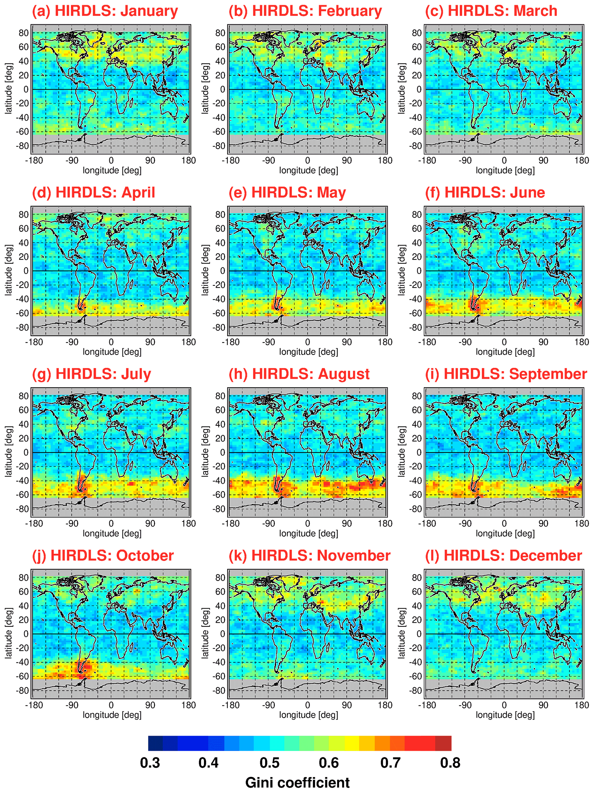
Figure 13 Same as Fig. 11 but for the Gini coefficients for HIRDLS gravity wave absolute momentum fluxes.

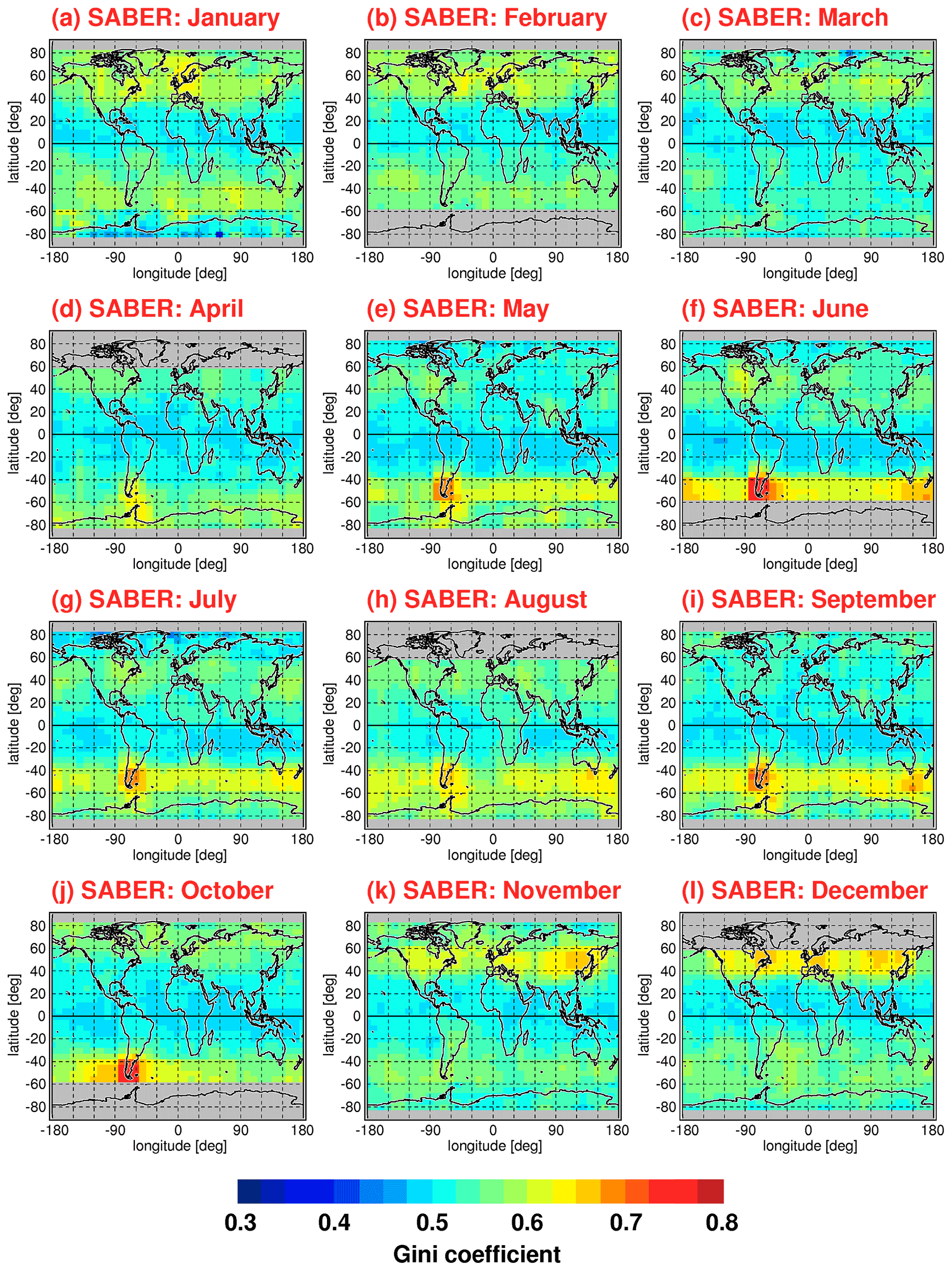
Figure 14 Same as Fig. 12 but for the Gini coefficients for SABER gravity wave absolute momentum fluxes and using a larger bin size of 20^∘ × 30^∘ (latitude × longitude).

As expected, the relative distributions of Gini coefficients for momentum fluxes are very similar to those for potential energies (see Figs. 11 and 12). However, Gini coefficients for gravity wave absolute momentum fluxes are generally higher than those obtained for potential energies. Indeed, stronger intermittency for distributions of momentum fluxes would be expected. Different from potential energies, momentum fluxes also depend on gravity wave horizontal and vertical wavelengths (see Eq. 7). As the wavelength distributions are also intermittent, this leads to the observed stronger intermittency of momentum fluxes. This effect was also seen for the PDFs in Sect. 4.2.

The relative distributions of the HIRDLS Gini coefficients for single calendar months in Fig. 13 are very similar to those previously derived by Wright et al. (2013) for HIRDLS absolute momentum fluxes (see the supplement of their paper). However, our Gini coefficients are considerably higher. Even the Gini coefficients for our gravity wave potential energies exceed the Gini coefficients for gravity wave absolute momentum fluxes in Wright et al. (2013).

The likely main reason for this difference in magnitude is differences in the gravity wave analysis technique. While we focus only on the strongest gravity wave at a given altitude in our study, the method used by Wright et al. (2013) selects for multiple waves in a given HIRDLS measurement, which typically identifies four discrete waves at any one measurement location (Wright and Gille, 2013; Wright et al., 2015). These additional waves usually have lower amplitudes and carry small momentum fluxes. This large population of relatively small absolute momentum fluxes will considerably pull down the level of intermittency, while relative variations in intermittency should be still dominated by the largest events.

Other possible reasons for the difference in magnitude are (1) the larger range of vertical wavelengths covered by our gravity wave analysis – vertical wavelengths of up to 25 km in our analysis compared with only up to 16 km in the analysis by Wright et al. (2013); (2) the fixed vertical resolution of 10 km of our analysis, which might give larger momentum fluxes for long vertical wavelength gravity waves due to the better vertical resolution; and (3) the fact that pairs of altitude profiles with nonmatching vertical wavelength are omitted in our method for deriving absolute momentum fluxes, whereas these events are retained in Wright et al. (2013) and may somewhat contribute to the abovementioned population of relatively small absolute momentum fluxes.

Remarkably, the magnitude of the Gini coefficients in Figs. 13 and 14 is very similar to values derived for absolute momentum fluxes obtained from superpressure balloons and high-resolution model simulations. For example, at altitudes of around 18 km, Gini coefficients I_g of 0.8 were obtained by Plougonven et al. (2013) over mountainous terrain in the Southern Hemisphere for the period from September 2005 until February 2006 in Weather Research and Forecast model (WRF) simulations. Similarly, a value of I_g=0.73 was obtained by Jewtoukoff et al. (2015) over mountainous terrain in the Southern Hemisphere during October 2010 from superpressure balloon observations. Over flat terrain (mostly ocean), values of I_g=0.34 to 0.58 (I_g=0.44 on average) and I_g=0.36 to 0.51 were obtained, respectively, by the same studies. In the tropics, values of I_g between 0.48 and 0.59 were obtained from superpressure balloon observations by Jewtoukoff et al. (2013). (These tropical values might, however, be somewhat high biased; see Corcos et al., 2021.)

The abovementioned values obtained from simulations and superpressure balloon observations compare very well to the values we obtain in our analysis from satellite data at 30 km altitude. For October, we obtain mean values of about I_g=0.7 (for HIRDLS) and I_g=0.65 (for SABER) over the southern tip of South America and the Antarctic Peninsula (see Figs. 13j and 14j). In the tropics, we find mean values between about 0.45 and 0.55 (see also Figs. 13 and 14).

Because the observational filters of limb sounders and superpressure balloons are very different, and the gravity wave spectrum in the simulations will also be different, the same waves are not necessarily being observed. Therefore, the agreement in Gini coefficient magnitudes suggests that, at least over a certain part of the gravity wave spectrum, the statistical distributions of momentum fluxes are similar.

6 Vertical evolution of intermittency diagnosed by Gini coefficients

In this section, we focus on SABER observations because these are available over a larger altitude range. Global distributions of gravity wave intermittency in the lower stratosphere still contain much information about the intermittency introduced by the gravity wave source processes. However, the vertical evolution of gravity wave intermittency is also of relevance, as the interaction of gravity waves with the background atmosphere during their propagation will have effect on the intermittency distribution. Some potential effects are as follows: (1) saturation and dissipation of large-amplitude gravity waves during their upward propagation should reduce the observed intermittency at high altitudes, (2) generation of secondary gravity waves when primary gravity waves dissipate (e.g., Vadas et al., 2018; Becker and Vadas, 2020) can alter the intermittency distribution, and (3) temporal changes in the background atmosphere will alter the propagation conditions for gravity waves and can, therefore, alter intermittency (either increase or decrease, e.g., Kim et al., 2021). Vertical changes in intermittency can, thus, also serve as a benchmark for the quality of the global distribution of gravity waves in models (i.e., whether sources, gravity wave propagation conditions, and all relevant processes of gravity wave physics are realistically simulated).

6.1 Zonal mean cross sections of Gini coefficients

In a first step, we investigate zonal mean distributions of median gravity wave momentum fluxes and of zonal mean Gini coefficients. These distributions are shown for SABER in Fig. 15 for medians of absolute momentum fluxes, and Fig. 16 shows the corresponding distributions for the zonal mean Gini coefficients.

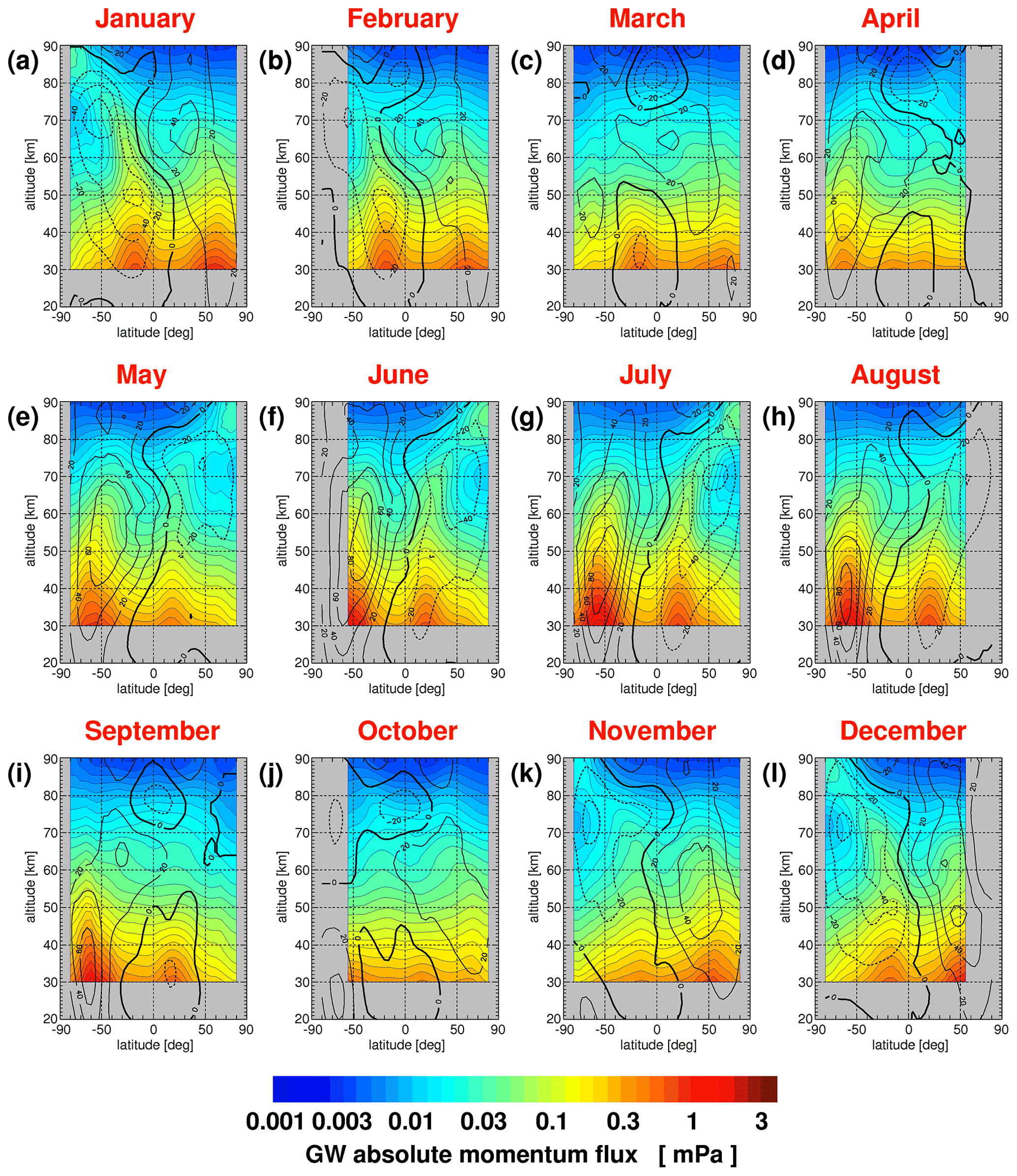
Figure 15 Multiyear mean zonal mean distributions of SABER median absolute gravity wave (GW) momentum fluxes for each calendar month. The averaging period is from January 2002 until October 2020. The plotted contour lines are zonal winds taken from the SPARC climatology of zonal winds (Swinbank and Ortland, 2003; Randel et al., 2002, 2004).

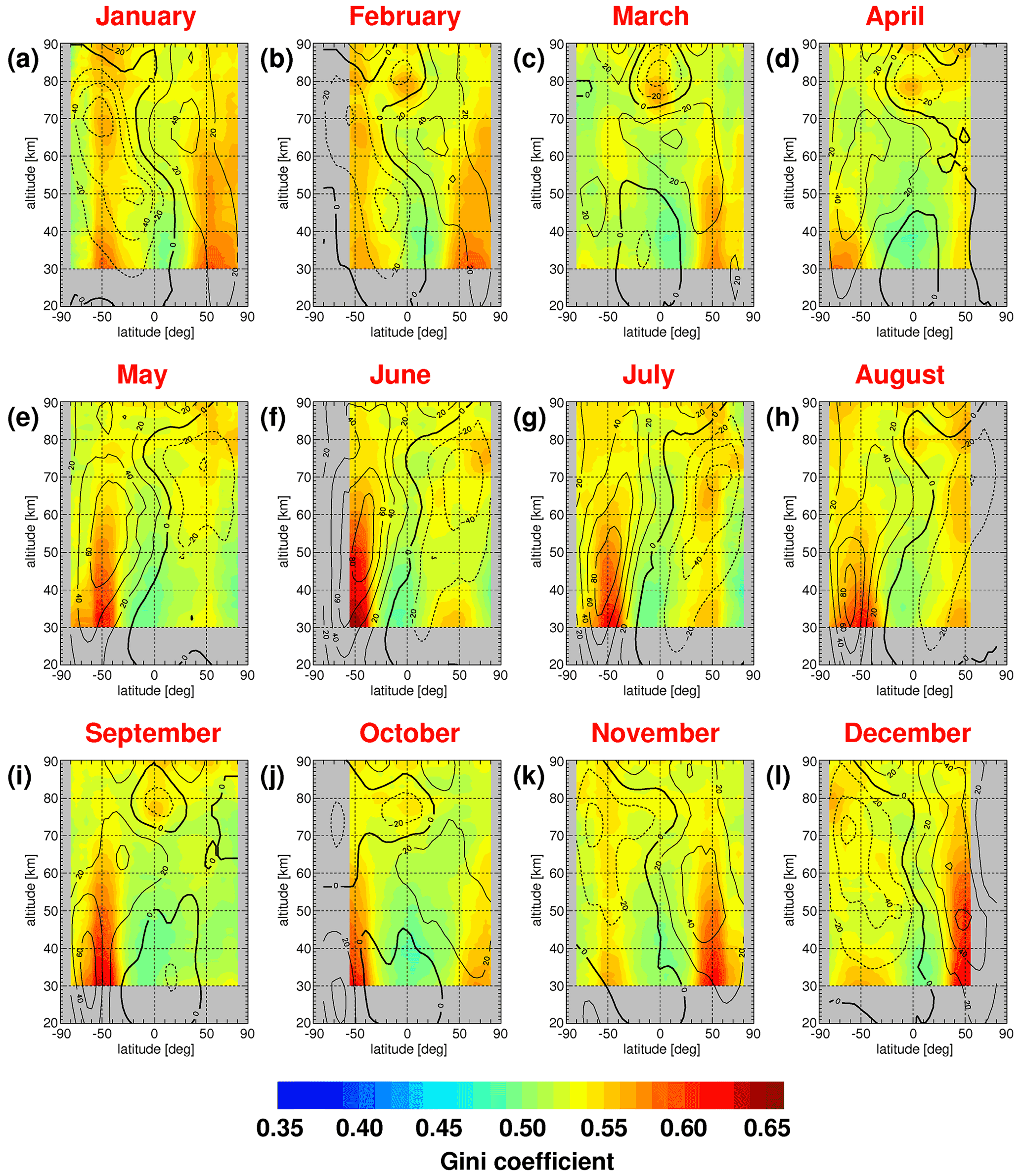
Figure 16 Same as Fig. 15 but for zonal mean Gini coefficients of the absolute momentum flux distributions.

For solstice conditions, enhanced gravity wave momentum fluxes are found in the polar night jets as well as in the subtropics of the respective summer hemisphere. Correspondingly, Gini coefficients are enhanced in the polar night jets. However, in the summer hemisphere, the highest Gini coefficients are found somewhat poleward of the momentum flux maximum, possibly because gravity waves are excited by deep convection more continuously in the tropics and subtropics but more sporadically at midlatitudes.

Interestingly, the altitude dependence of Gini coefficients displays characteristic latitudinal differences. In the tropics, Gini coefficients at low altitudes are generally low, and they increase with altitude, mainly in the mesosphere. At low altitudes, Gini coefficients should still be dominated by the intermittency of the gravity wave source processes. This indicates that gravity waves with horizontal wavelengths longer than 100–200 km in the tropics that can be detected by limb sounders are continuously excited (e.g., by mesoscale convective systems), and exceedingly strong events are rare, resulting in relatively low intermittency. This was already seen from the low-latitude PDFs in Figs. 7 and 9.

With increasing altitude, the intermittency of gravity waves (and thus the Gini coefficients) should be more and more dominated by the gravity wave propagation conditions that are governed by variations in the background atmosphere (i.e., the background winds and static stability). The background atmosphere in the tropical stratosphere is dominated by the relatively slow QBO of the zonal winds. Of course, the QBO will modulate the distribution of gravity waves (e.g., Ern et al., 2014). However, during a single month (our multiyear means are based on single-month distributions) these variations will not add much intermittency to the intermittency caused by the gravity wave source processes. At higher altitudes, however, the background atmosphere in the tropics is dominated by the SAO of the zonal wind as well as by atmospheric tides. The timescales of these variations are much shorter than that of the QBO, and, accordingly, on a monthly basis, these variations and the corresponding variations in the gravity wave distribution (e.g., Preusse et al., 2001; Ribstein and Achatz, 2016; Ern et al., 2015, 2021) should add intermittency to the monthly means. This could explain the increase in intermittency with altitude in the tropics as well as the intermittency maxima that are found at low latitudes around 80 km altitude around the equinoxes (see Fig. 16). This will be investigated in more detail in Sect. 6.2.

In the respective winter hemisphere, at low altitudes, we find enhanced Gini coefficients in the region of the polar night jet. As was seen from Figs. 1–4 and 11–14, enhanced gravity wave activity and Gini coefficients in this season and these regions are likely caused by orography and jet-related gravity wave sources. Strikingly, Gini coefficients stay high until reaching about the altitude of maximum eastward winds. Above this altitude, Gini coefficients decrease considerably. One possible explanation for this finding could be that high-amplitude mountain waves and high-amplitude jet-generated waves will gradually saturate due to amplitude growth in the reduced background density and dissipate while propagating upward (see also Alexander et al., 2016). As these waves contribute considerably to increased intermittency at low altitudes, dissipation of these waves should lead to a decrease in the Gini coefficients with altitude. This was already indicated by the SABER PDFs at different altitudes shown in Fig. 6. Consequently, gravity wave hot spots should become increasingly less prominent at high altitudes. Again, this will be investigated in more detail in Sect. 6.2.

In the respective summer hemisphere, midlatitude Gini coefficients are somewhat higher than in the tropics, but peak values are considerably lower than peak values found in the in the polar night jets. There is some altitude variation with somewhat enhanced values at low altitudes, possibly caused by intermittent gravity wave sources. Further, Gini coefficients are somewhat enhanced in the region of maximum westward winds in the summertime mesospheric wind jets, which hints at some effect of changes in gravity wave propagation conditions.

6.2 Horizontal distributions at different altitudes

Next, using SABER data, we will investigate how the global distributions of gravity wave momentum fluxes and Gini coefficients evolve with increasing altitude. For this, we focus on periods around the solstices in order to investigate the changes in the very characteristic global distributions during these periods. In addition, we want to avoid the months of TIMED yaw maneuvers. For these reasons, we selected the calendar months of August and December: Fig. 17 shows the global distributions of SABER median gravity wave momentum fluxes (Fig. 17a, c, e, g) and the corresponding distributions of Gini coefficients (Fig. 17b, d, f, h) at altitudes of 30 km (Fig. 17a, b), 50 km (Fig. 17c, d), 70 km (Fig. 17e, f), and 80 km (Fig. 17g, h) for the calendar month of August. Figure 18 shows the same but for the calendar month of December. Again, the distributions shown are arithmetic means over the years 2002 until 2020.

Figure 17 Global distributions of (a, c, e, g) SABER median absolute gravity wave momentum fluxes (MF) at altitudes of 30, 50, 70, and 80 km for the calendar month of August as well as (b, d, f, h) the corresponding global distributions of Gini coefficients. Again, the global distributions are arithmetic means obtained over the period from January 2002 to October 2020.

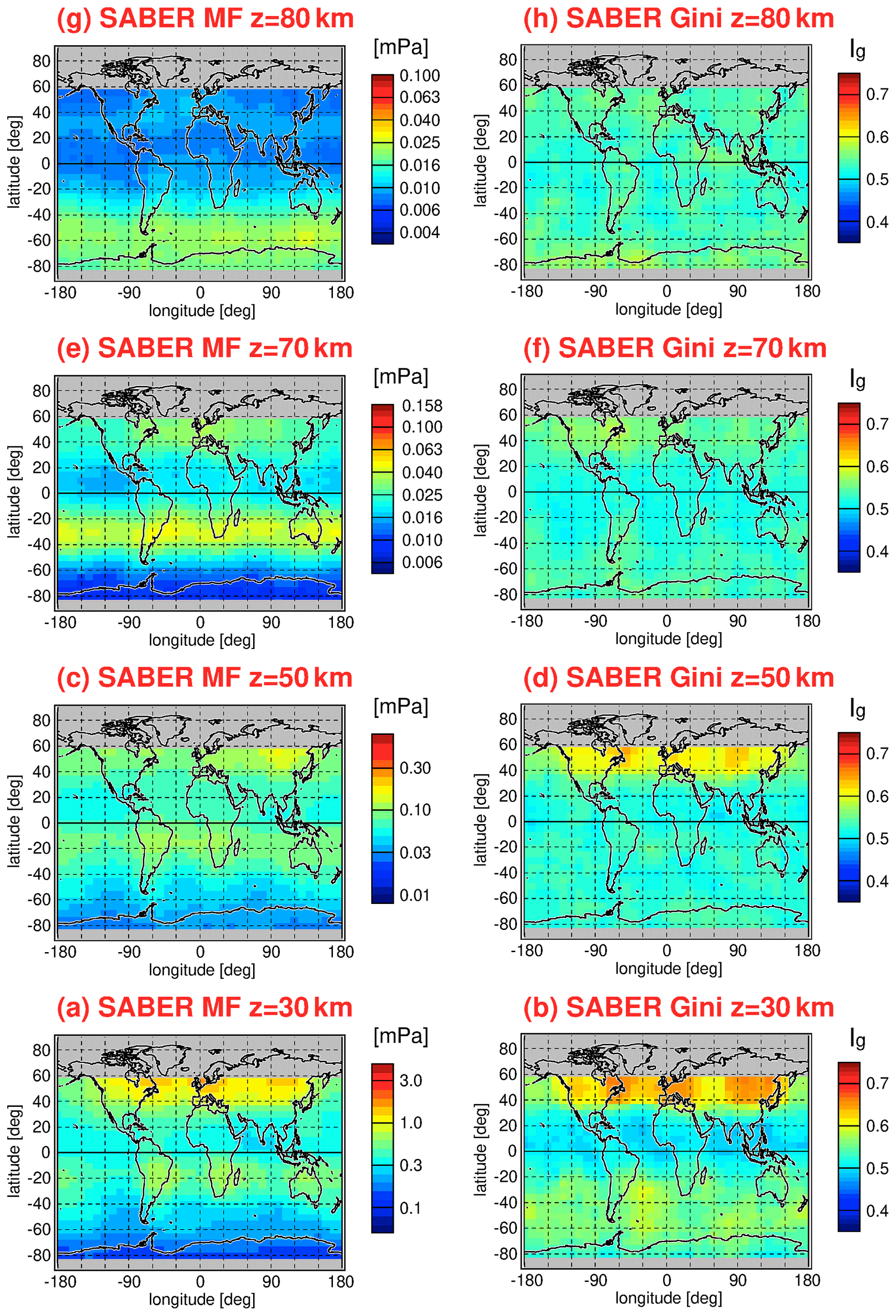
Figure 18 Same as Fig. 17 but for the calendar month of December.

As can be seen from Figs. 17 and 18, at an altitude of 30 km, the global distributions of momentum fluxes and Gini coefficients show the characteristic features of enhanced momentum fluxes and Gini coefficients at middle and high latitudes of the respective winter hemisphere (that are governed by the respective polar night jet), low Gini coefficients in the tropics, and intermediate Gini coefficients in the summer hemisphere subtropics and midlatitudes. Particular enhancements of momentum fluxes and Gini coefficients are found in August over South America and the Antarctic Peninsula, and in December over Northeast America, Europe, and Northeast Asia. Further, enhancements of momentum fluxes are found in the subtropics of the respective summer hemisphere.

At an altitude of 50 km, these distributions are still visible, but the specific features are much less pronounced. At 70 km altitude, the momentum flux distributions still exhibit some of these characteristic features. The range of the logarithmic color scale, however, was much reduced to make these structures visible. In contrast, the global distribution of Gini coefficients is almost flat and attains intermediate values of about 0.5, which means an increase in the Gini coefficients in the tropics and a reduction in the Gini coefficients at middle and high latitudes in the respective winter hemisphere.

For December, this is also the case at 80 km altitude; however, in August, at 80 km altitude, some structures start to emerge, with enhanced Gini coefficients in the tropics and enhanced values at midlatitudes in the Northern Hemisphere. The seasonality of these structures might be related to seasonal variations in the background atmosphere, which can lead to modulations of the gravity wave distribution. Possible candidates are the SAO in the tropics and atmospheric tides. Further investigation of this effect is, however, beyond the scope of this study. At 80 km, the momentum flux distribution also shows some structure. However, it is not clear whether the strong enhancement of momentum fluxes at high southern latitudes during August is reliable, as enhanced noise of the SABER temperature retrieval is expected in the cold summer mesopause region (see also Ern et al., 2018).

Changes in the global distribution of Gini coefficients with altitude were investigated previously, for example, by Alexander et al. (2016) based on momentum fluxes of the gravity waves resolved by the Kanto GCM in the Southern Hemisphere. The Kanto model resolves gravity waves with horizontal wavelengths longer than about 200 km (e.g., Watanabe et al., 2008; Sato et al., 2012), which roughly agrees with the range of horizontal wavelengths seen by infrared limb sounders. For July, at 50 hPa (about 21 km altitude), Alexander et al. (2016) found that Gini coefficients at middle and high southern latitudes are about 0.55 for oceanic regions, while Gini coefficients reach peak values as high as 0.7 to 0.9 in the regions above South America and the Antarctic Peninsula (that are dominated by mountain waves). At higher altitudes of 0.1 hPa (about 65 km), this difference between regions is strongly reduced to about 0.55 to 0.6 for the oceanic regions and 0.6 to 0.65 for the mountain wave regions, respectively (see their Figs. 5b and 6). In the subtropics, Gini coefficients increase from about 0.45–0.50 at 50 hPa to about 0.55 at 0.1 hPa.

In January, the Gini coefficients obtained by the Kanto model are about 0.45 to 0.50 throughout the Southern Hemisphere at 21 km altitude. Gini coefficients increase only slightly between 21 km (50 hPa) and 65 km (0.1 hPa) altitude; see Figs. 5a and 10a in Alexander et al. (2016).

Qualitatively, these results are similar to our findings: an increase in the Gini coefficients with altitude at low latitudes as well as and an increasingly uniform distribution of Gini coefficients with increasing altitude. Even the magnitudes of Gini coefficients are in good agreement between Alexander et al. (2016) and our study.

Changes in the Gini coefficients with altitude were also investigated by Wright et al. (2013) using HIRDLS absolute momentum fluxes. Of course, as mentioned in Sect. 5.2.2, there is some difference in the magnitude of Gini coefficients between Wright et al. (2013) and our study. However, there is still qualitative agreement with respect to some of the relative variations. For example, in the tropics, Wright et al. (2013) observed an increase in the Gini coefficients with altitude at altitudes above about ∼ 40 km, similar to our study. In other regions, the agreement with our study is less clear; for example, in Wright et al. (2013), intermittency increases or stays constant with altitude in oceanic regions, and it either slightly increases or decreases with altitude in mountain wave regions.

7 Summary and discussion

Intermittency of the global distribution of gravity waves is an important effect that can be caused, for example, by gravity wave source processes or varying gravity wave propagation conditions (i.e., variability in the background atmosphere). Although intermittency has an effect on where gravity waves dissipate and, thus, contribute to the driving of the global atmospheric circulation, intermittency is often neglected in gravity wave parameterizations. This means that the variability in gravity wave drag that is introduced by gravity wave intermittency is missing in many models.

As there are only few observations of gravity wave intermittency and its variation with altitude, we used global observations of gravity wave potential energies and of gravity wave absolute momentum fluxes, by the High-Resolution Dynamics Limb Sounder (HIRDLS) and Sounding of the Atmosphere using Broadband Emission Radiometry (SABER) infrared limb sounding satellite instruments, to investigate the global distribution of gravity wave intermittency and its evolution with altitude. For HIRDLS, we use observations from the period from January 2005 to February 2008; for SABER, we use the period from January 2002 until October 2020. The determination of gravity wave potential energies and absolute momentum fluxes from temperature observations follows the method described, for example, in Ern et al. (2018).

First, we derived probability density functions (PDFs) of gravity wave potential energies and absolute momentum fluxes in different regions. For a better comparability between different regions, we normalized the single values of potential energies and momentum fluxes by their monthly global distribution of median values. In agreement with previous observations (e.g., Baumgaertner and McDonald, 2007; Hertzog et al., 2008, 2012; Plougonven et al., 2013; Wright et al., 2013), we found that the PDFs of gravity wave potential energies and momentum fluxes roughly follow lognormal distributions. Already, this fact is an indication for strong intermittency associated with the distribution of gravity waves. However, there are important differences, depending on region and altitude.

In the stratosphere, we find that the PDFs over the Southern Ocean during austral winter closely follow lognormal distributions, in agreement with previous observations by HIRDLS and superpressure balloons (Hertzog et al., 2012). Our satellite observations show that the same is also the case at northern middle and high latitudes during boreal winter.

From previous observations by superpressure balloons and from corresponding high-resolution model simulations in Southern Hemisphere regions that are dominated by mountain waves during austral winter, it is expected that PDFs of absolute momentum fluxes even exceed a lognormal distribution at high momentum flux values (e.g., Hertzog et al., 2012; Plougonven et al., 2013). This is also found in our satellite observations, although less pronounced, which is likely an observational filter effect: satellite infrared limb sounders are sensitive only to gravity waves with horizontal wavelengths > 100–200 km (e.g., Preusse et al., 2002; Ern et al., 2018) and might, therefore, miss events of very strong momentum fluxes. Further, low biases of momentum fluxes may be introduced by (1) the HIRDLS and SABER sensitivity functions for gravity waves; (2) the satellite sampling that only allows one to estimate the apparent gravity wave horizontal wavelength parallel to the satellite track, which always overestimates the true gravity wave horizontal wavelength; and (3) short horizontal wavelength gravity waves may be undersampled, which also leads to an overestimation of the true gravity wave horizontal wavelength. A more detailed discussion of the observational filter of infrared limb sounders is given, for example, by Preusse et al. (2009a) and Trinh et al. (2015).

The PDFs over Scandinavia during boreal winter do not show this pronounced enhancement at high momentum flux values. Possibly, the gravity waves observed in this region are a mixture of highly intermittent mountain waves and less intermittent jet-generated gravity waves.

The PDFs in the tropics and in the respective summer hemisphere are quite different from those observed at middle and high latitudes during winter. The tropical and summer hemisphere PDFs are considerably skewed toward low values: low momentum flux values are more abundant, and high momentum fluxes are less abundant than suggested by a lognormal distribution. This is in agreement with previous findings by, for example, Ern et al. (2014), and this finding may be relevant for a more realistic simulation of the QBO.

At high altitudes, the PDFs are increasingly more skewed towards low values because the tail of the distribution at high momentum flux values is much reduced, likely due to dissipation of high-amplitude gravity waves at already relatively low altitudes.

The PDFs that we find for gravity wave potential energies in the same regions are qualitatively very similar to those found for absolute momentum fluxes. The main difference is that potential energy PDFs are much narrower. Indeed, the intermittency of potential energies should be lower than the intermittency of momentum fluxes because the gravity wave horizontal and vertical wavelengths are also included in the calculation of momentum fluxes, which will introduce further variability and, thus, intermittency.

While PDFs can give a complete picture of the magnitude distribution of a selected parameter, they require a large number of observations to give reliable results, and a display of global distributions is not easily possible. For this reason, intermittency coefficients were developed that provide a measure of intermittency for a given dataset as a single number (see also Hertzog et al., 2012; Plougonven et al., 2013). Recently, the Gini coefficient (Gini, 1912) has most widely been used to characterize the intermittency of gravity wave distributions. Therefore, we derived global distributions of Gini coefficients for each multiyear mean calendar month for both HIRDLS and SABER gravity wave potential energies and absolute momentum fluxes. Again, the values of potential energies and momentum fluxes were normalized by the monthly global distributions of medians to avoid biases of derived Gini coefficients by horizontal gradients within the latitude–longitude bins used to calculate the Gini coefficients. This is particularly important for SABER momentum fluxes because relatively large bins of 20^∘ × 30^∘ (latitude × longitude) have to be used to obtain sufficient statistics.

As already indicated by the PDFs, intermittency in the stratosphere is weakest in the tropics, followed by the summertime subtropics and summertime midlatitudes. Intermittency is strongest at winter hemisphere middle and high latitudes, with the strongest values over regions that are known for the strong activity of mountain waves, such as South America, the Antarctic Peninsula, New Zealand, or Scandinavia. The magnitude of our Gini coefficients is in good agreement with previous observations by superpressure balloons (e.g., Plougonven et al., 2013; Jewtoukoff et al., 2013, 2015) and with previous results obtained using high-resolution models (e.g., Plougonven et al., 2013; Alexander et al., 2016). Values of Gini coefficients obtained previously from HIRDLS observations are considerably lower (see the supplement of Wright et al., 2013). Possible reasons are differences in the method for deriving gravity wave momentum fluxes as well as a larger range of vertical wavelengths covered in our work. This shows the importance of using similar gravity wave analysis techniques if intermittency (e.g., PDFs or Gini coefficients) is to be directly compared.

In the extratropics, where intermittency is strongest at low altitudes, intermittency decreases with altitude. In the tropics, however, intermittency increases with altitude. Consequently, the global distribution of Gini coefficients is relatively flat at altitudes around 70 km and displays only weak variations around a value of 0.5. These findings are in good agreement with results of the Kanto model in the Southern Hemisphere (Alexander et al., 2016). In the tropics, our findings are also qualitatively in agreement with previous results obtained from HIRDLS observations (Wright et al., 2013).

In regions of strong intermittency at low altitudes, the reduction in the Gini coefficients with altitude may be related to the dissipation of high-amplitude gravity waves, as these waves saturate more quickly while propagating upward. Increases in the Gini coefficients with altitude (particularly in the tropics) may be related to varying gravity wave propagation conditions. In the tropics, this may be caused, for example, by the SAO of the background winds as well as by atmospheric tides (e.g., Ern et al., 2015, 2021; Ribstein and Achatz, 2016), as the timescales of these variations are close to, or shorter than, 1 month, which is the time interval used in our study to collect observations for calculating Gini coefficients.

It should be mentioned that the results obtained in our study apply only to the part of the gravity wave spectrum that is visible for infrared limb sounders. Our study roughly covers gravity waves with horizontal wavelengths longer than about 100–200 km as well as vertical wavelengths in the range of 2–25 km for HIRDLS and 4–25 km for SABER. Approximate sensitivity functions are given, for example, in Ern et al. (2018). An improvement of this sensitivity could be achieved, for example, by future 3D observations and tomographic temperature retrievals (e.g., Preusse et al., 2009a; Ungermann et al., 2010; Song et al., 2017, 2018; Gumbel et al., 2020). It should be noted that the level of intermittency depends on the part of the gravity wave spectrum considered. In particular, intermittency could be stronger if only short horizontal wavelength gravity waves are considered. This is indicated, for example, in the recent studies by Kim et al. (2021) or Corcos et al. (2021). Further, intermittency could be different if timescales much shorter than 1 month were used to collect data for calculating PDFs or Gini coefficients.

Appendix A: The effect of normalization on SABER Gini coefficient distributions

In our study, we normalize gravity wave potential energy or momentum fluxes at a given altitude by their spatially varying monthly global distributions of medians. One of the main reasons for doing so is to account for horizontal gradients within the latitude–longitude bins that are used for calculating either PDFs or Gini coefficients. Strong horizontal gradients within a given bin can lead to spurious increases in intermittency. Here, as an example, in Fig. A1, we show the global distribution of the SABER Gini coefficients determined in the same way as for Fig. 14 but without normalization.

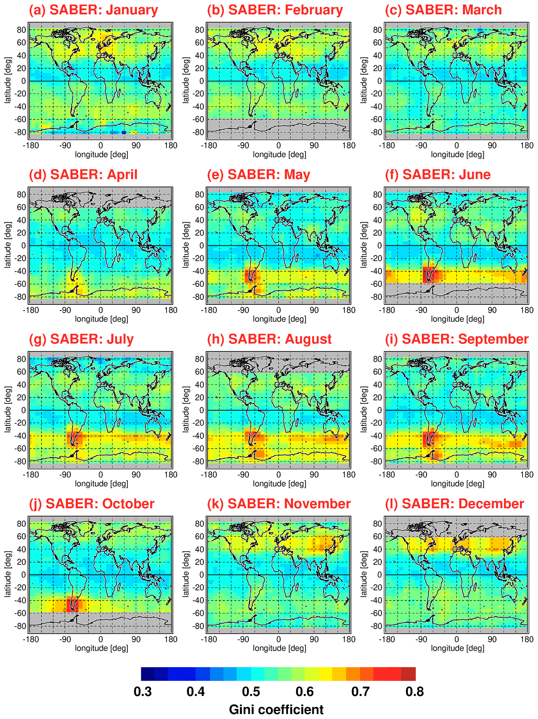
Figure A1 Same as Fig. 14, in that the Gini coefficients for SABER gravity wave absolute momentum fluxes for each multiyear mean calendar month are shown using a relatively large bin size of 20^∘ × 30^∘ (latitude × longitude), but without normalization of gravity wave momentum fluxes before calculating the Gini coefficients.

By comparing Figs. 14 and A1, it can be seen that two bands of strong intermittency (high Gini coefficients) are found at around 45 and 70^∘ S in the Southern Hemisphere, particularly in the months July to September. These bands of enhanced Gini coefficients coincide with the strong gradients of momentum fluxes seen in Fig. 4g–i at the same latitudes. After applying the normalization, these enhancements disappear (see Fig. 14), which results in a much better agreement with the relative distributions of Gini coefficients that are based on smaller latitude–longitude bins (e.g., Fig. 12) that are much less affected by horizontal gradients.