the Creative Commons Attribution 4.0 License.
the Creative Commons Attribution 4.0 License.
 | 25 Nov 2022
Global seasonal distribution of CH2Br2 and CHBr3 in the upper troposphere and lower stratosphere
Markus Jesswein
Rafael P. Fernandez
Lucas Berná
Alfonso Saiz-Lopez
Jens-Uwe Grooß
Ryan Hossaini
Eric C. Apel
Rebecca S. Hornbrook
Elliot L. Atlas
Donald R. Blake
Stephen Montzka
Timo Keber
Tanja Schuck
Thomas Wagenhäuser
Andreas Engel
Bromine released from the decomposition of short-lived brominated source gases contributes as a sink of ozone in the lower stratosphere. The two major contributors are CH2Br2 and CHBr3. In this study, we investigate the global seasonal distribution of these two substances, based on four High Altitude and Long Range Research Aircraft (HALO) missions, the HIAPER Pole-to-Pole Observations (HIPPO) mission, and the Atmospheric Tomography (ATom) mission. Observations of CH2Br2 in the free and upper troposphere indicate a pronounced seasonality in both hemispheres, with slightly larger mixing ratios in the Northern Hemisphere (NH). Compared to CH2Br2, CHBr3 in these regions shows larger variability and less clear seasonality, presenting larger mixing ratios in winter and autumn in NH midlatitudes to high latitudes. The lowermost stratosphere of SH and NH shows a very similar distribution of CH2Br2 in hemispheric spring with differences well below 0.1 ppt, while the differences in hemispheric autumn are much larger with substantially smaller values in the SH than in the NH. This suggests that transport processes may be different in both hemispheric autumn seasons, which implies that the influx of tropospheric air (“flushing”) into the NH lowermost stratosphere is more efficient than in the SH. The observations of CHBr3 support the suggestion, with a steeper vertical gradient in the upper troposphere and lower stratosphere in SH autumn than in NH autumn. However, the SH database is insufficient to quantify this difference. We further compare the observations to model estimates of TOMCAT (Toulouse Off-line Model of Chemistry And Transport) and CAM-Chem (Community Atmosphere Model with Chemistry, version 4), both using the same emission inventory of Ordóñez et al. (2012). The pronounced tropospheric seasonality of CH2Br2 in the SH is not reproduced by the models, presumably due to erroneous seasonal emissions or atmospheric photochemical decomposition efficiencies. In contrast, model simulations of CHBr3 show a pronounced seasonality in both hemispheres, which is not confirmed by observations. The distributions of both species in the lowermost stratosphere of the Northern and Southern hemispheres are overall well captured by the models with the exception of southern hemispheric autumn, where both models present a bias that maximizes in the lowest 40 K above the tropopause, with considerably lower mixing ratios in the observations. Thus, both models reproduce equivalent flushing in both hemispheres, which is not confirmed by the limited available observations. Our study emphasizes the need for more extensive observations in the SH to fully understand the impact of CH2Br2 and CHBr3 on lowermost-stratospheric ozone loss and to help constrain emissions.
- Article
(4939 KB) - Full-text XML
-
Supplement
(3259 KB) - BibTeX
- EndNote


Reactive gases containing chlorine and bromine are very efficient in destroying stratospheric ozone in catalytic reaction cycles. The relative efficiency of bromine is 60–65 times higher than that of chlorine (e.g. Sinnhuber et al., 2009; WMO, 2018). A more recent study reports a 74 times higher efficiency of bromine (Klobas et al., 2020). Thus, although the amount of bromine in the stratosphere is much smaller than that of chlorine, bromine plays an important role in stratospheric ozone chemistry. Major contributors to stratospheric bromine are the four major halons H-1211 (CBrClF2), H-1301 (CBrF3), H-1202 (CBr2F2), and H-2402 (CBrF2CBrF2), all originating from anthropogenic sources. Furthermore, methyl bromide (CH3Br) is a major contributor, which has both natural and anthropogenic sources. Additionally, the so-called “very short-lived substances” (VSLSs), with lifetimes shorter than 6 months, can contribute bromine to the stratosphere and thus lead to ozone loss. Bromine VSLSs (Br-VSLSs in the following) contributed about a quarter to stratospheric bromine in 2016 with a total of 5 (3–7) ppt (parts per trillion) (Engel et al., 2018). The contribution is partly in the form of organic source gases (source gas injection; SGI) providing 2.2 (0.8–4.2) ppt Br and in inorganic form as photochemically decomposed species (product gas injection; PGI) with 2.7 (1.7–4.2) ppt Br (Engel et al., 2018). Once in the lowermost stratosphere (LMS), released bromine from VSLSs can affect the ozone abundance and distribution. Especially in the midlatitude LMS, bounded by the 380 K potential temperature surface at the top and the extratropical tropopause at the bottom (e.g. Hoor et al., 2005), bromine-driven ozone loss cycles gain importance (e.g. Daniel et al., 1999; Salawitch et al., 2005). It is also a region where ozone changes have a relatively large radiative effect (Hossaini et al., 2015, and references therein).
Transport of source gases into the LMS can occur via different pathways. Transport associated with the global-scale stratospheric Brewer–Dobson circulation (BDC) brings older air from the stratospheric overworld into the upper troposphere and lower stratosphere (UTLS) via the deep branch with long transit times, as well as air from the tropics and subtropics into the UTLS via the shallow branch with shorter transit times (Birner and Bönisch, 2011). On the other hand, air can be transported directly into the LMS via the extratropical tropopause by troposphere-to-stratosphere transport (TST). Kunkel et al. (2019) describe in more detail the processes for stratosphere–troposphere exchange (STE) in the midlatitudes, for example due to Rossby wave breaking and tropopause folds along jet streams. Furthermore, Kunkel et al. (2019) suggested that air masses potentially enter the stratosphere in ridges of baroclinic waves at the anticyclonic side of the jets above the outflow of warm conveyor belts (whereby the significance of this process still needs to be assessed). Previous studies estimated that the contribution of extratropical tropospheric air to the LMS shows a pronounced seasonality. Hoor et al. (2005) used CO in situ measurements to infer a fraction of 35 % extratropical tropospheric air in winter and spring LMS composition over Europe, whereas the fraction rises to 55 % in summer and autumn. A similar seasonality but with much higher extratropical fractions was found by Bönisch et al. (2009) using in situ measurements of CO2 and SF6. Extratropical tropospheric fractions of up to 90 % were found in October and the lowest fraction below 20 % in April. Hegglin et al. (2009) used O3, H2O, and CO measurements from the Atmospheric Chemistry Experiment Fourier Transformation Spectrometer (ACE-FTS) on Canada's SCISAT-1 satellite to investigate the global behaviour of the extratropical tropopause transition layer (ExTL), which is the finite chemical transition layer across the tropopause and into the LMS. Major findings were a shallower transition layer in the Southern Hemisphere (SH) with a weaker troposphere–stratosphere transport compared to the Northern Hemisphere (NH) and an overall smaller seasonal variation. Hegglin and Shepherd (2007) showed that “flushing” of the LMS with younger air from the tropics is most evident in NH summer and autumn and is weaker in the SH. These results are confirmed by the CO tracer distribution in Hegglin et al. (2009).
The different transport paths have an influence on the distribution of Br-VSLSs, especially in the LMS of each hemisphere. This study focuses on bromoform (CHBr3) and dibromomethane (CH2Br2), which are the most abundant Br-VSLSs. The local lifetime of CH2Br2 ranges from 150 to 890 d and that of CHBr3 between 17 to 88 d, depending on location and season (see Sect. 4, Table 3 for seasonally resolved local lifetimes). The main sources of these Br-VSLSs are open-ocean and coastal regions via the metabolism of marine organisms such as phytoplankton and macro-algae (e.g. Carpenter and Liss, 2000; Quack et al., 2007; Leedham et al., 2013). Sturges et al. (1993) and Abrahamsson et al. (2018) suggested that winter sea ice could potentially be an additional source of Br-VSLSs. Anthropogenic sources are water chlorination (e.g. Worton et al., 2006; Maas et al., 2021) and industrial discharge of chlorinated effluents to seawater (Quivet et al., 2022; Maas et al., 2019; Hamed et al., 2017; Boudjellaba et al., 2016; Sam Yang, 2001). The contribution of treated water may have an impact on a local scale only, and the significance of theses sources on a global scale remains unclear (e.g. Quivet et al., 2022; Liu et al., 2011). Studies of the observation-based distribution, especially when looking at stratospheric input of Br-VSLSs, have focused predominantly on the tropics and the NH. The current best estimates of tropical tropopause values of CH2Br2 and CHBr3 are given in Engel et al. (2018) ranging from 0.81 (0.59–0.98) ppt to 0.64 (0.32–0.89) ppt CH2Br2 from the level of 0 clear-sky radiative heating (LZRH) to the tropical tropopause (TTP) and 0.36 (0.05–0.72) ppt to 0.19 (0.01–0.54) ppt CHBr3 from LZRH to TTP (Wofsy, 2011; Sala et al., 2014; Navarro et al., 2015; Pan et al., 2017). A recent study by Keber et al. (2020) reported aircraft measurements of Br-VSLSs at the tropopause and LMS in NH midlatitudes to high latitudes during winter and late summer to early autumn. They reported systematically higher mixing ratios of CHBr3 at the extratropical tropopause than those at the TTP. A similar, although less pronounced feature was found for CH2Br2. This increase was more pronounced in winter, when lifetimes increase at higher latitudes. In addition, Keber et al. (2020) compared their observations with model estimates using different emission scenarios. Although no scenario was able to capture the tropical and extratropical values from their observations, the Ordóñez et al. (2012) scenario showed an overall good agreement, especially for CH2Br2.
As Keber et al. (2020) already pointed out, there are still some knowledge gaps regarding the distribution of the Br-VSLSs in the upper atmosphere, as they only show observations of the NH in winter and late summer to early autumn. Especially the data coverage in the SH is sparse. It is expected that the distribution of the Br-VSLSs in the SH may differ from the NH distribution, due to fewer source regions like coastal ocean regions. Here we expand the analysis of Keber et al. (2020) to a global view of the two major Br-VSLSs. For that, besides using the observations already used in Keber et al. (2020), namely the High Altitude and Long Range Research Aircraft (HALO) missions TACTS (Transport and Composition in the Upper Troposphere/Lowermost Stratosphere), PGS, and WISE (Wave-driven ISentropic Exchange), we also use observations from the southern hemispheric HALO mission SouthTRAC (Southern Hemisphere Transport, Dynamics, and Chemistry) from September to November 2019. Furthermore, we use observations from the HIAPER Pole-to-Pole Observations (HIPPO) mission and the Atmospheric Tomography (ATom) mission, both of which include data from the Northern and Southern hemispheres, to investigate the global seasonal distribution of the Br-VSLSs. Observations are compared with two global models, namely CAM-Chem (Community Atmosphere Model with Chemistry, version 4) and TOMCAT (Toulouse Off-line Model of Chemistry And Transport), both using the same emission scenario of Ordóñez et al. (2012). In Sect. 2, we give a brief overview of the missions and instruments used for this analysis, followed by an introduction to the meteorological data and the models against which we compare the observations in Sect. 3. The distribution of CH2Br2 and CHBr3 from observations and model simulations is discussed in Sect. 4. We start with the broader global distribution by presenting seasonal zonal mean mixing ratios from both hemispheres from the ground to the lower stratosphere, moving on to a closer look at near-tropopause mixing ratios, and finally focus on the vertical distribution in the midlatitudes of NH and SH. Lastly, we summarize the conclusion and provide an outlook in Sect. 5.
2.1 HALO missions
In this work, we use data from four missions conducted with the High Altitude and Long Range Research Aircraft (HALO). HALO is a Gulfstream V (GV) aircraft and can reach altitudes of up to 15 km. The first mission is the TACTS (Transport and Composition in the Upper Troposphere/Lowermost Stratosphere) mission, conducted in August and September 2012 with flights covering an area from the Cabo Verde islands to the Norwegian archipelago of Spitsbergen and over Europe and the Atlantic Ocean. The base of all flights was Oberpfaffenhofen (Germany) (Fig. 1, blue tracks). The second mission was PGS, consisting of three sub-missions: POLSTRACC (Polar Stratosphere in a Changing Climate), GW-LCYCLE (Investigation of the Life cycle of gravity waves), and SALSA (Seasonality of Air mass transport and origin in the Lowermost Stratosphere). The mission took place from December 2015 to March 2016 with flights mainly in the Arctic and covering Greenland, the North Atlantic, and Europe. Flights were conducted from Oberpfaffenhofen (Germany) and from Kiruna (Sweden) (Fig. 1, purple tracks) (Oelhaf et al., 2019). The third mission was the WISE (Wave-driven ISentropic Exchange) mission between September and October 2017. Flights were conducted mainly from Shannon (Ireland), covering an area above the Atlantic Ocean and western Europe (Fig. 1, green tracks). Finally, the SouthTRAC (Southern Hemisphere Transport, Dynamics, and Chemistry) mission took place from September to November 2019. It is the only one of the four HALO missions that covers the SH. In addition to the scientific transfer flights, which departed from Oberpfaffenhofen (Germany) via the Cabo Verde islands to South America, all other flights took place from Rio Grande (Argentina). Flights of the SouthTRAC mission cover the southern Pacific and southern Atlantic oceans near South America and Antarctica (Fig. 1, orange tracks).
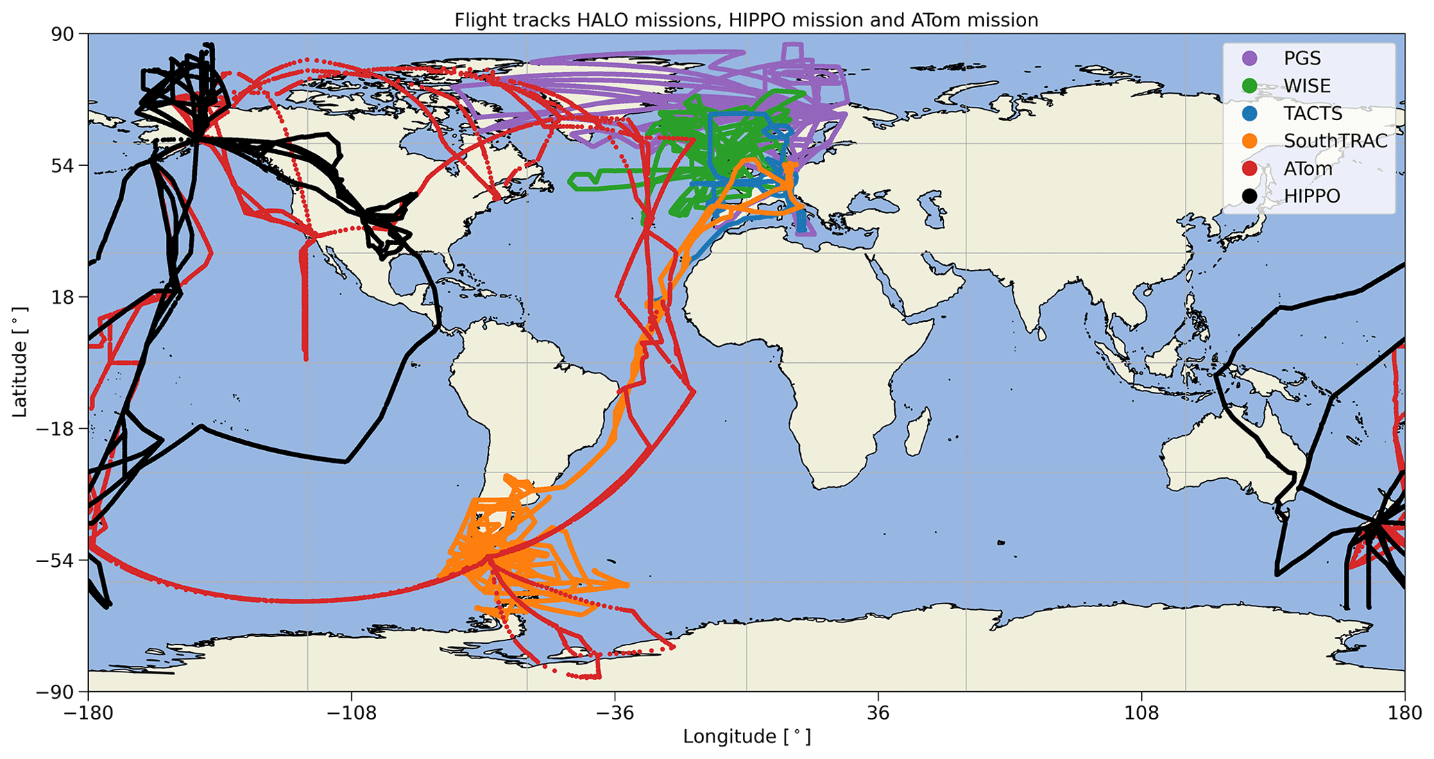
Figure 1Flight tracks of the HALO missions TACTS (blue), WISE (green), PGS (purple), and SouthTRAC (orange) as well as flight tracks of the HIPPO mission (black) and ATom mission (red).
Data from the Gas chromatograph for Observational Studies using Tracers (GhOST) in situ instrument were used in this analysis. The instrument has two channels. The first channel couples an isothermally operated gas chromatograph (GC) with an electron capture detection (ECD) (GhOST-ECD), and the second channel couples a temperature-programmed GC with a quadrupole mass spectrometer (MS) (GhOST-MS) (see Jesswein et al. (2021) and references therein). For the SouthTRAC campaign, the GhOST-MS ionization mode was changed from negative chemical ionization (NCI) to electron impact ionization (EI) to record broader mass spectra, leading to different detection limits for the Br-VSLSs compared to previous campaigns. In this work, only measurements of the MS channels are used. The measurements of CH2Br2 and CHBr3 are on the NOAA-2003 scale, thus consistent with NOAA/ESRL observations.
2.2 HIPPO mission
The HIPPO mission measured cross sections of trace gases over the Pacific Basin and North American mainland (170–80∘ W) (Fig. 1 black tracks), covering a latitudinal range from the North Pole (85∘ N) to the coastal region of Antarctica (65∘ S) (Wofsy, 2011). The mission was split into seasonal segmented deployments, which took place in January 2009 (HIPPO-1), October to November 2009 (HIPPO-2), March to April 2010 (HIPPO-3), June to July 2011 (HIPPO-4), and August to September 2011 (HIPPO-5). The platform used for the observations was the NSF/NCAR High-performance Instrumented Airborne Platform for Environmental Research (HIAPER) Gulfstream V (GV) aircraft.
Data from two whole air samplers (WASs) were combined in this analysis. The University of Miami operated the Advanced Whole Air Sampler (AWAS), storing air samples in pressurized stainless steel canisters (Atlas, 2016). The second sampler operated during HIPPO was the NOAA Whole Air Sampler (NWAS), which stores samples in pressurized glass flasks. Subsequently, the samples were analysed using ground-based laboratory GC–MS (gas chromatograph–mass spectrometer) systems. Results from both laboratories were provided on a scale consistent with NOAA/ESRL ground-based station results (see Hossaini et al., 2013, 2016).
2.3 ATom mission
The ATom mission was split into four parts, which took place in July to August 2016 (ATom-1), January to February 2017 (ATom-2), September to October 2017 (ATom-3), and April to May 2018 (ATom-4). Thus, all seasons were covered within a 2-year time period. In each season, flights started and ended in Palmdale (California, USA) with a route to the western Arctic, south to the South Pacific, east to the Atlantic, and north to Greenland, returning across central North America (Wofsy et al., 2021) (Fig. 1, red tracks). The platform for the ATom mission was the NASA DC-8 aircraft, which is capable of reaching an altitude of around 12 km (Thompson et al., 2022).
As with the HIPPO mission, data from two WASs were used for this analysis. The University of Carlifornia – Irvine (UC-Irvine) research group operated one whole air sampler (hereafter referred to as WAS), storing air in stainless steel canisters. Samples were analysed in the laboratory using GC with flame ionization detection (FID), ECD, and MS (Barletta et al., 2019). In addition, the NOAA/GML's Programmable Flask Package Whole Air Sampler (PFP) was operated using glass flasks. The air samples were analysed at the NOAA's Global Monitoring Division laboratory for trace gases by GC-MS and at the Institute of Arctic and Alpine Research (INSTAAR) Stable Isotope Lab for isotopes of methane. Beside the two WASs, the NCAR Trace Organic Gas Analyzer (TOGA) was operated during ATom. TOGA is an in situ instrument, combining a GC with an MS (Apel et al., 2015), similar to the GhOST-MS. Asher et al. (2019) used ATom-2 observations among others to improve estimates of short-lived halocarbon emissions during summer from the Southern Ocean using airborne observations. The two whole air samplers and the TOGA instrument shared approximately half of the sampling period, generally presenting a good correlation and consistency in mole fractions for CH2Br2 and CHBr3 (Asher et al., 2019).
3.1 TOMCAT
The TOMCAT (Toulouse Off-line Model of Chemistry And Transport) is an Eulerian offline three-dimensional chemistry transport model (CTM) (Chipperfield, 2006; Monks et al., 2017). The model uses a hybrid vertical sigma–pressure coordinate (σ–p) with 60 vertical levels from the ground up to around 60 km. The horizontal resolution was set to (latitude × longitude). The CTM is forced by meteorological fields (winds, temperature, and humidity) taken from the European Centre for Medium-Range Weather Forecasts ERA5 reanalysis (Hersbach et al., 2020). The internal model step was 30 min and monthly means of the tracers are generated for this study. A similar setup was previously used to study NH Br-VSLSs in Keber et al. (2020), beside using ERA-Interim data instead of ERA5. In addition, the configuration used here reads an offline monthly varying climatological OH concentration field, developed for the TransCom-CH4 project (Patra et al., 2011). In this study, the VSLS emission scenario of Ordóñez et al. (2012), which includes monthly variability in emissions, was used with TOMCAT. Model output is available for the period from 2009 to 2019.
3.2 CAM-Chem
CAM-Chem (Community Atmosphere Model with Chemistry, version 4) is a three-dimensional chemistry climate model (CCM) and a component of the NCAR Community Earth System Model (CESM) (Lamarque et al., 2012). The WACCM (Whole Atmosphere Community Climate Model) physics module for the stratosphere is included, and it uses the chemical mechanism of MOZART (Model for OZone and Related chemical Tracers) with different possibilities of complexity for tropospheric and stratospheric chemistry. The model includes a detailed treatment of tropospheric Br-VSLS sources and chemistry described in Fernandez et al. (2014) and Fernandez et al. (2017). The horizontal resolution was set to (latitude × longitude) and 56 hybrid vertical levels from the surface to around 40 km. The model setup is similar to the one used in Navarro et al. (2015), using the NASA Goddard Global Modeling and Assimilation Office (GMAO) GEOS5-generated meteorology. The model step was 5 min but monthly means of the tracers are used for this study. As with the TOMCAT model, the monthly varying emission scenario of Ordóñez et al. (2012) was used, with fixed emissions of the VSLSs during the whole modelling period (available from 2009–2019).
3.3 Meteorological data
Aeroplanes modified for scientific observations are equipped with on-board instruments to gather meteorological and aircraft parameters along the flight tracks. In addition, local tropopause information along the flight tracks as well as equivalent latitude were derived using the Chemical Lagrangian Model of the Stratosphere (CLaMS) (e.g. Grooß et al., 2014) with underlying ECMWF reanalysis. For the SouthTRAC, PGS, HIPPO, and ATom mission, the underlying meteorological field are taken from the ERA5 reanalysis, whereas for TACTS and WISE, the underlying fields are from the ERA-Interim reanalysis (Dee et al., 2011).
For this work, the potential vorticity (PV)-based dynamical tropopause is used (e.g. Gettelman et al., 2011). The commonly used value of 2 PVU (potential vorticity unit) was used for the dynamical tropopause; this condition was replaced by the potential temperature level of 380 K in the tropics when the 2 PVU level is above (e.g. Keber et al., 2020; Jesswein et al., 2021). We additionally used the same PV-based climatological tropopause information as in Keber et al. (2020), which is based on the ERA-Interim reanalysis.
4.1 Analysis methods
In the course of this work, we progressively move from a more global view of the distribution of the tracers to a more detailed view of the UTLS in the midlatitudes of both hemispheres. For the global view (Sect. 4.2), we use latitude as the horizontal coordinate and pressure as the vertical coordinate and thus get a detailed perspective of the troposphere from the ground up to the tropopause and the LMS. As we then look more closely at the area around the tropopause and into the stratosphere, we change the vertical coordinate using potential temperature (Θ) and potential temperature difference to the local tropopause (ΔΘ) instead of pressure (starting from Sect. 4.3). Transport in the free atmosphere is predominantly isentropic, making Θ a very useful coordinate. Furthermore, Θ allows for better vertical resolution as it increases more rapidly with height in stable layers. Finally, the focus moves towards the UTLS of the midlatitudes in the course of the analysis (Sect. 4.4). We switch from the examination in latitude only to a combined coordinate already used in Keber et al. (2020) and Jesswein et al. (2021). Latitude is used for tropospheric observations, whereas equivalent latitude is used for stratospheric ones. The equivalent latitude (Butchart and Remsberg, 1986) is a commonly used horizontal coordinate for studying tracers in the stratosphere and assigns PV to latitude based on the area (of the polar cap) enclosed by the specific isopleth of PV on a given potential temperature contour (Pan et al., 2012). The combined coordinate is referred to as equivalent latitude*. In all sub-analyses (Sects. 4.2–4.4), the observations are compared with the model data. The model results are only used for the years and months for which observations are available and have been zonally averaged (consistent with Keber et al., 2020).
4.2 Altitude–latitude cross sections
We combined the measurements from the different missions, leaving aside that the Br-VSLSs may have shown a weak positive trend (e.g. tropical mean 0.017 ± 0.012 ppt Br per decade for 1979–2013 from Tegtmeier et al., 2020). Observations and model results were split by season (DJF: December, January, February; MAM: March, April, May; JJA: June, July, August; SON: September, October, November). The data are binned in 10∘ latitude intervals from 90∘ S to 90∘ N. In the vertical we have binned the data between 1000 and 50 hPa into 20 bins. The bin size decreases logarithmically with increasing altitude and thus lower pressure. Thus, the size of the bins varies from about 180 hPa near the ground to 8.5 hPa in the lower stratosphere, which corresponds to an altitude resolution of about 1.3 km.
Figures 2 and 3 show the distributions of CH2Br2 and CHBr3 for the observations (a–d), the TOMCAT model (e–h), the CAM-Chem model (i–l), and the differences between the respective model and the observations (m–t). The merged observational data set allows for a comprehensive representation of the tropospheric distribution except for the southern high latitudes (greater than 70∘ S) in summer and winter. Furthermore, the LMS of both hemispheres is much better covered by observations in spring and autumn.
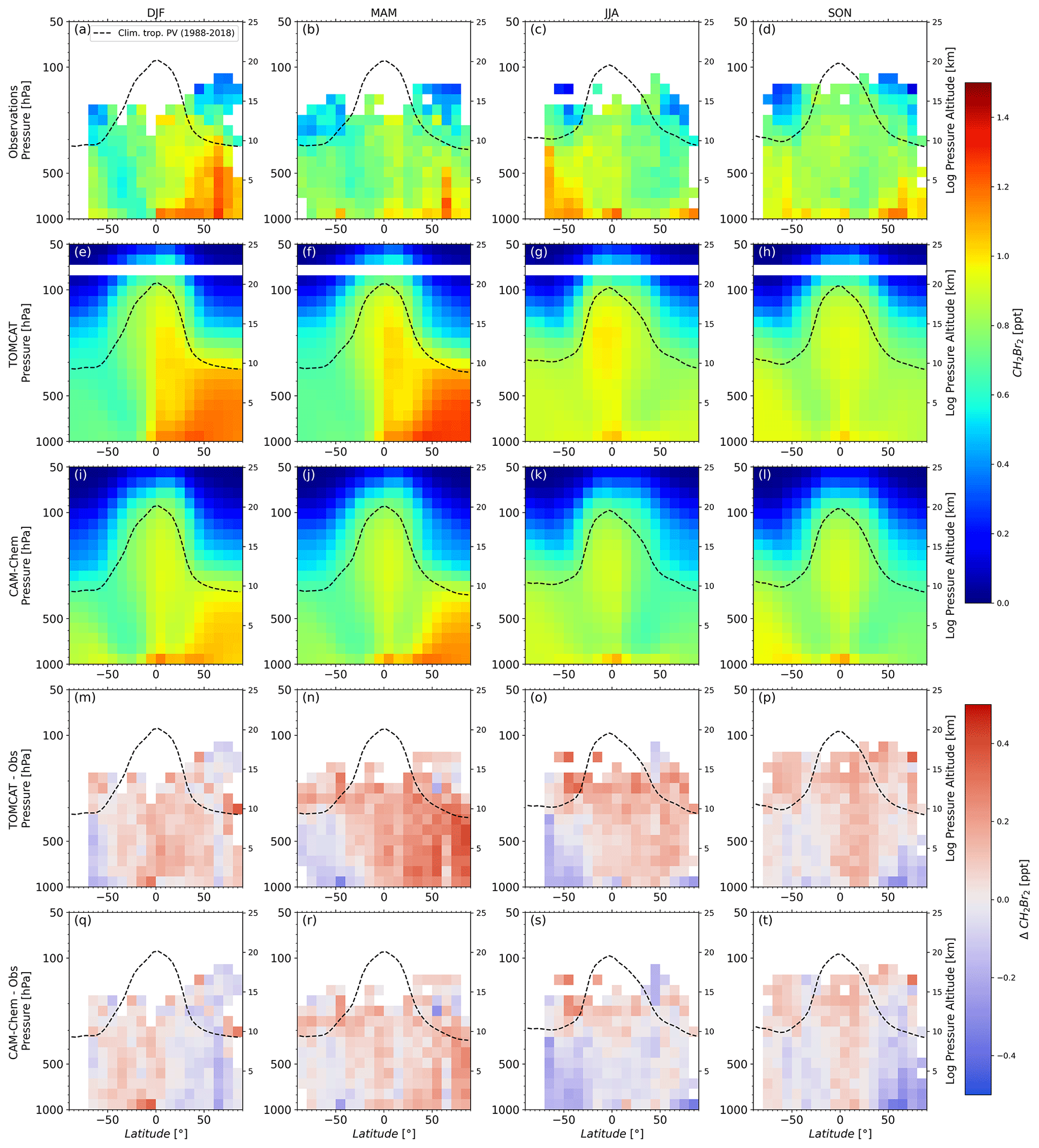
Figure 2Altitude–latitude cross section of CH2Br2. The data are separated by season and displayed as a function of latitude and pressure. Top row (a–d) shows observational data. Second and third row (e–h and i–l) show model results of TOMCAT and CAM-Chem, respectively. Fourth and fifths row (m–p and q–t) show differences between the respective model and the observations. The dynamical tropopause (dashed lines) has been derived from the ERA-Interim reanalysis, providing a climatological (1988–2018) zonal mean tropopause. The slightly coarser vertical resolution of TOMCAT combined with the bin size leads to missing TOMCAT data between 68 and 80 hPa.
The distributions of CH2Br2 in the troposphere (Fig. 2a–d) show a general increase in mixing ratios with increasing latitude, which is most pronounced in hemispheric winter. Increased mixing ratios almost reach the tropopause for this season. The tropospheric distributions show a clear seasonality in both hemispheres with the largest values observed in hemispheric winter and the smallest values in hemispheric summer in the lower troposphere. There is a slight asymmetry towards generally higher mixing ratios in the NH, particularly for the 70∘ N bin. The NH has more coastal regions, which are assumed to be one of the main sources of Br-VSLSs, which could explain the asymmetry of tropospheric mixing ratios. A rather striking difference between the NH and SH is observed in the LMS in autumn and spring. While the distribution of CH2Br2 in hemispheric spring is quite similar in both hemispheres, the distribution in hemispheric autumn differs with smaller values in the SH compared to the NH. Mixing ratios above the subtropical and extratropical tropopause are up to 0.3 ppt smaller in the SH. High mixing ratios of tropospheric tracers in the LMS observations during NH autumn have been explained by a strong influx of tropospheric air during NH summer and autumn (flushing of the LMS) (e.g. Hoor et al., 2005; Bönisch et al., 2009). It could be argued that this is an indication of the different strength of tropospheric air mixing into the LMS of the two hemispheres. The subtropical jet acts as a transport barrier and Konopka et al. (2015) diagnosed a hemispheric asymmetry of the subtropical jet with a most pronounced weakening in the NH summer (see Fig. 1 and references in Konopka et al., 2015).
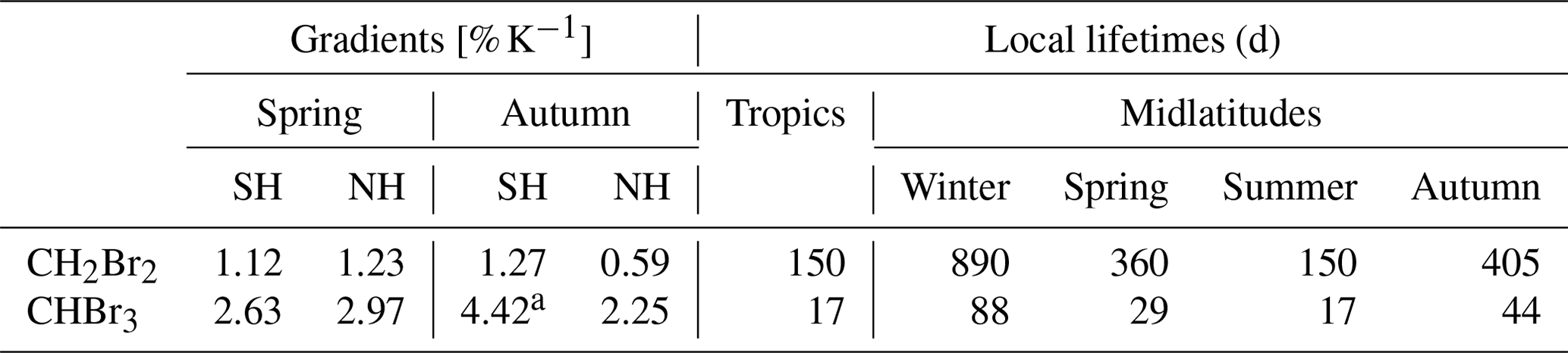
Even though SH observations are available for all seasons from the different missions, the SH database remains much smaller than the NH database. Unfortunately, MAM measurements during ATom-4 show quite large differences between the results from TOGA and both whole air samplers (WAS and PFP) but only for observations of the SH LMS. Figure 4 displays the altitude–latitude cross section of the observations for MAM, taking all observations (a) and thus being similar to Fig. 2b as well as using all observations but only TOGA measurements from ATom (b) and using all observations but only the whole air samplers for ATom (c). Although there is little difference in the rest of the atmosphere due to the use of TOGA or WAS/PFP, the difference in the SH LMS during MAM is clear (see Fig. 4 observations inside red rectangles). Using the TOGA data (Fig. 4b), values are larger in the range of around 0.4–0.8 ppt, which would suggest a flushing of the LMS similar to that in northern hemispheric autumn (e.g. Bönisch et al., 2009). Values are much smaller when using WAS and PFP data (Fig. 4c) below around 0.4 ppt. This would indicate a strong isolation of the SH lower stratosphere. Indeed, Shuckburgh et al. (2009) investigated a strong seasonal cycle in the strength of the barriers at the subtropical jet, where in MAM in the SH, mixing follows a mostly zonal pattern and the subtropical jet acts as a barrier. They further stated that observed mixing is of the greatest magnitude in the NH in any season. The representation of the southern hemispheric UTLS in MAM is based on fewer observations than, e.g., southern hemispheric UTLS in spring where the SouthTRAC campaign took place. The SouthTRAC campaign contributes to a substantial portion of the spring UTLS observations in the SH. For a more meaningful result especially in SH autumn, but also in winter and summer, further measurements are necessary and should be a focus of future campaigns.
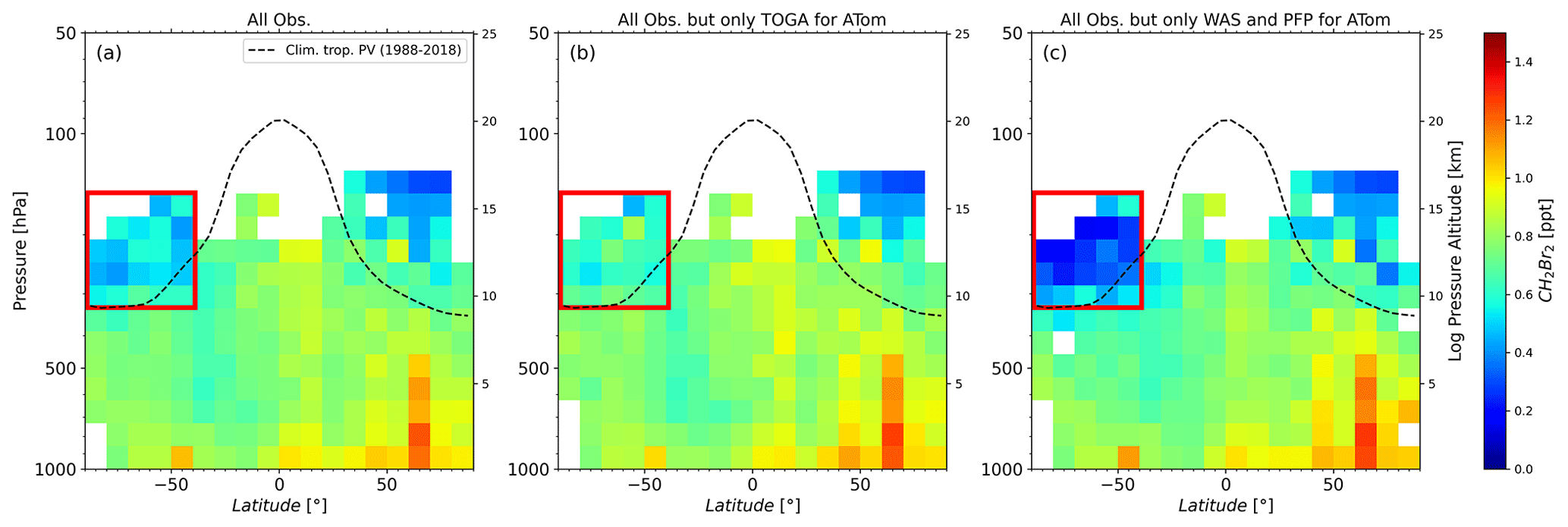
Figure 4Altitude–latitude cross section of CH2Br2 for March, April, and May. Panel (a) presents the distribution of CH2Br2 as in Fig. 2, whereas in (b) data from all missions were used, but only TOGA observations from ATom were included, and in (c) data from all missions were used, but only WAS and PFP observations from ATom were included. The red rectangle indicates the region where observations from different techniques differed substantially from one another.
The model results show a general good agreement to the observations in the annual mean. Positive or negative bias to the observations are not very pronounced or consistent. Instead, negative or positive bias is dependent on season and latitude. For the case of CH2Br2, the largest lower-tropospheric values in the NH observations are in winter, whereas models show the largest values in spring. This may arise from a possible incorrect seasonal representation in the Ordóñez et al. (2012) emission scenario. Furthermore, TOMCAT values in the free troposphere are larger than in CAM-Chem, despite using the same emission scenario. Thus, overestimation in MAM in the NH is larger within TOMCAT with differences to observations of up to about 0.4 ppt. Both models underestimate NH high-latitude values of CH2Br2 in SON by up to 0.3 ppt. Hossaini et al. (2016) showed a comparison of different models and ground-based stations in which the models do not reproduce the seasonality at coastal stations such as Mace Head (Ireland) (see Fig. 3 therein). The observations used in this work were conducted predominantly over ocean and coastal regions (e.g. nearshore bases such as during the WISE campaign) and may have similar signatures to the coastal stations shown in Hossaini et al. (2016). Neither model shows the pronounced seasonal pattern of CH2Br2 in the SH with elevated values in the southern hemispheric winter. This may be due to the emission scenario of Ordóñez et al. (2012), which was used in both models. The top–down emission estimates of the bromocarbons in the Ordóñez et al. (2012) scenario are based on aircraft campaigns and some available observations in the marine boundary layer, most of which are from the NH. Ordóñez et al. (2012) already identified the issue regarding the emission flux estimates in the SH as a consequence of missing aircraft observations in the SH (especially south of 40∘ S for all seasons). In addition, the Ordóñez et al. (2012) emission inventory does not consider Br-VSLSs arising from sea ice regions, which are possible sources of Br-VSLSs according to, e.g., Abrahamsson et al. (2018).
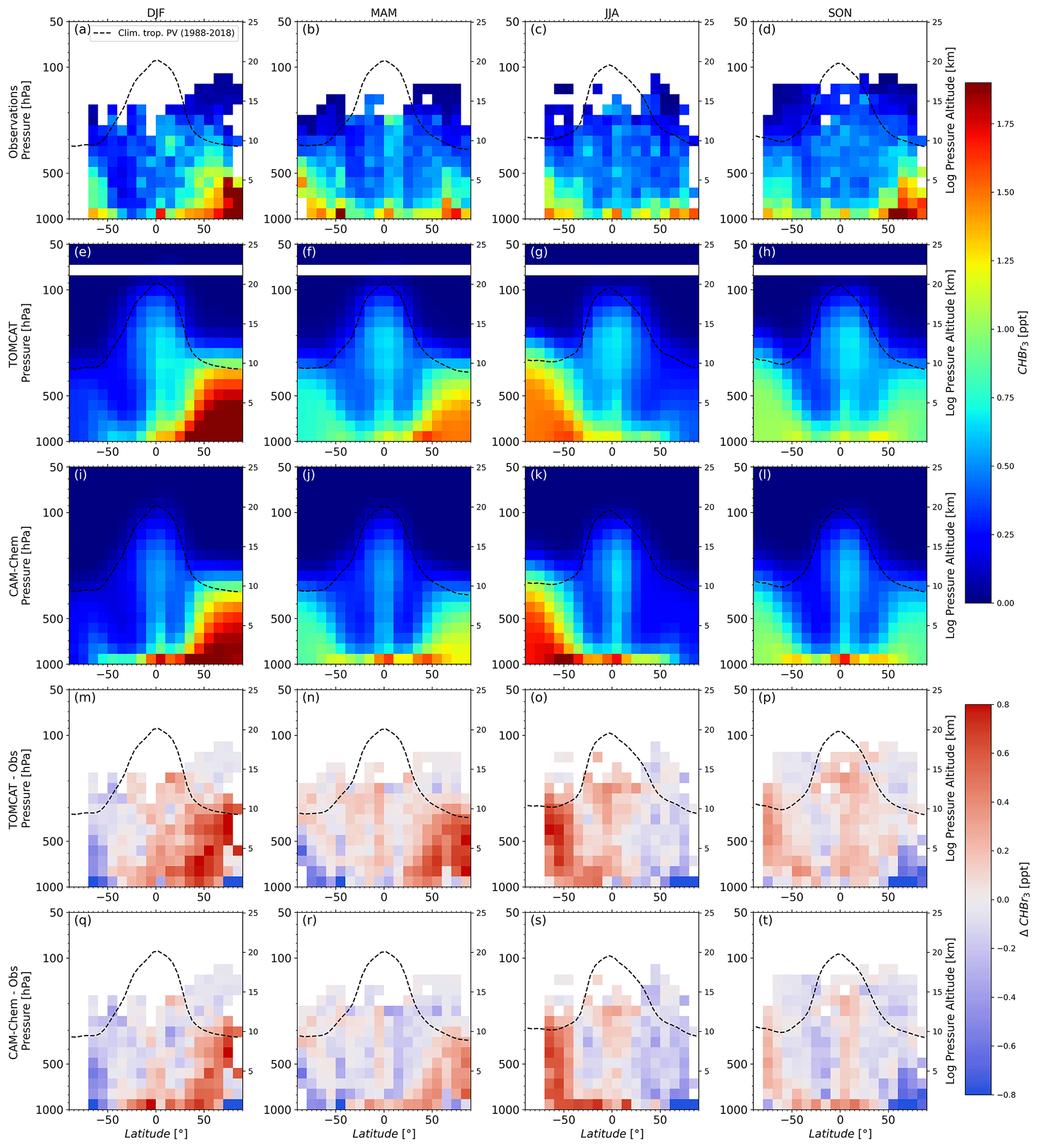
As noted before, CHBr3 has a much shorter atmospheric lifetime than CH2Br2. Consequently, the global tropospheric distributions from the observations of CHBr3 show larger variability and a less pronounced seasonality. Jia et al. (2019) used simulations to demonstrate that uniform background emissions of CHBr3 from the ocean result in a highly variable distribution in the atmosphere with larger values in regions of convergence or low wind speed and that the impact of localized elevated emissions on the distribution varies significantly from campaign to campaign. Thus, the interpretation of CHBr3 airborne observations is challenging. Nonetheless, the NH shows larger values in autumn and winter compared to spring and summer, a feature that is captured by both models, although the modelled wintertime maxima are more pronounced than in the observations and much less pronounced in autumn. Near-ground observations, however, may not be representative as they are largely from coastal areas. Based on the limited existing observations in the SH, the seasonality is not very pronounced with slightly smaller values in summer high latitudes and slightly larger near-ground values in autumn followed by winter. SH high-latitude ground-based NOAA/GML measurements presented in Hossaini et al. (2016) like the one from Cape Grim (Tasmania, Australia) and the Palmer Station (Antarctica), which are on a consistent scale as aircraft measurements, e.g. from PFP, also show a less pronounced seasonality. Furthermore, measurements of these stations reveal that models did not capture the observed seasonality for coastal stations (see Fig. 3 in Hossaini et al., 2016). Observations and model comparison from this study demonstrate a similar discrepancy as seen in Hossaini et al. (2016) at high latitudes of the SH with an underestimation in summer and autumn, where differences for tropospheric observations range between about 0.2 and 0.6 ppt, and overestimation mainly in winter high latitudes which reaches up to 0.8 ppt. Both models overestimate NH tropospheric values in winter and spring by up to 0.8 ppt except for near-ground values at high latitudes, which are much larger in the observational data (2–5 ppt difference to the observations above 80∘ N). In summer and autumn, the models underestimate high-latitude values (differences to observations of about 0.2 ppt and up to 0.9 ppt near the ground). Especially in the NH there is a larger frequency of observations over the northern Atlantic Ocean (see Fig. 1). For example, the flights of the WISE campaigns took place predominantly from Shannon (Ireland), close to known coastline source regions of CHBr3, which may have a greater influence on the atmospheric distribution than photochemical decay (e.g. Carpenter et al., 2005; Hossaini et al., 2016). CHBr3 lower-stratospheric values are close to 0, as this substance has a shorter lifetime and is faster decomposed compared to CH2Br2. Model estimates of TOMCAT and CAM-Chem overall agree well within the LMS of both hemispheres.
4.3 Upper-tropospheric latitudinal distribution
Trace gases can enter the extratropical UTLS through several pathways. Beside the downward transport from the stratospheric overworld, there is a two-way exchange across the extratropical tropopause and an isentropic exchange, often in the vicinity of the subtropical jet (e.g. Gettelman et al., 2011, and references therein). The amount of total bromine likely differs depending on how and where air enters the LMS and, consequently, the characteristics of the contributing input regions.
To investigate the distributions of the two major Br-VSLSs in the upper troposphere as a function of latitude, we binned the observational data according to latitude and to potential temperature relative to the local tropopause. Only data in the 10 K range below the local dynamical tropopause are included, to characterize the possible input region. For the models, only data in the 10 K range below the climatological PV-based tropopause are included. Data have been separated into low latitudes (0–30∘), midlatitudes (30–60∘), and high latitudes (60–90∘) for both hemispheres. Results for CH2Br2 and CHBr3 are listed in Tables 1 and 2, respectively, and the hemispheric winter CH2Br2 results are shown in Fig. 5 (graphical representations of the other seasons and seasonal cycle of each latitudinal band can be found in the Supplement). Engel et al. (2018) reported typical tropical tropopause mixing ratios compiled from different measurement campaigns with mixing ratios in the upper tropical tropopause layer (upper TTL) of 0.73 (0.43–0.94) ppt CH2Br2 and 0.28 (0.02–0.64) ppt CHBr3.
Table 1Averaged mole fractions (median in parts per trillion, ppt) of CH2Br2 and their corresponding range (25th to 75th percentiles) at high latitudes (60–90∘), midlatitudes (30–60∘), and low latitudes (0–30∘) in the upper troposphere, e.g. within 10 K below the local dynamical tropopause for the Northern and Southern hemispheres.
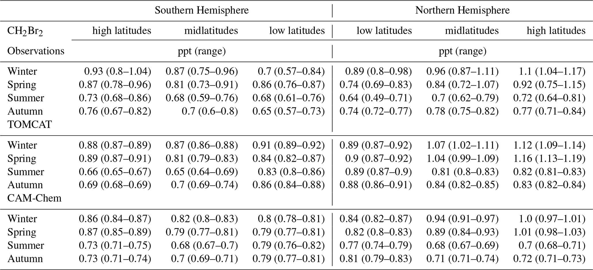
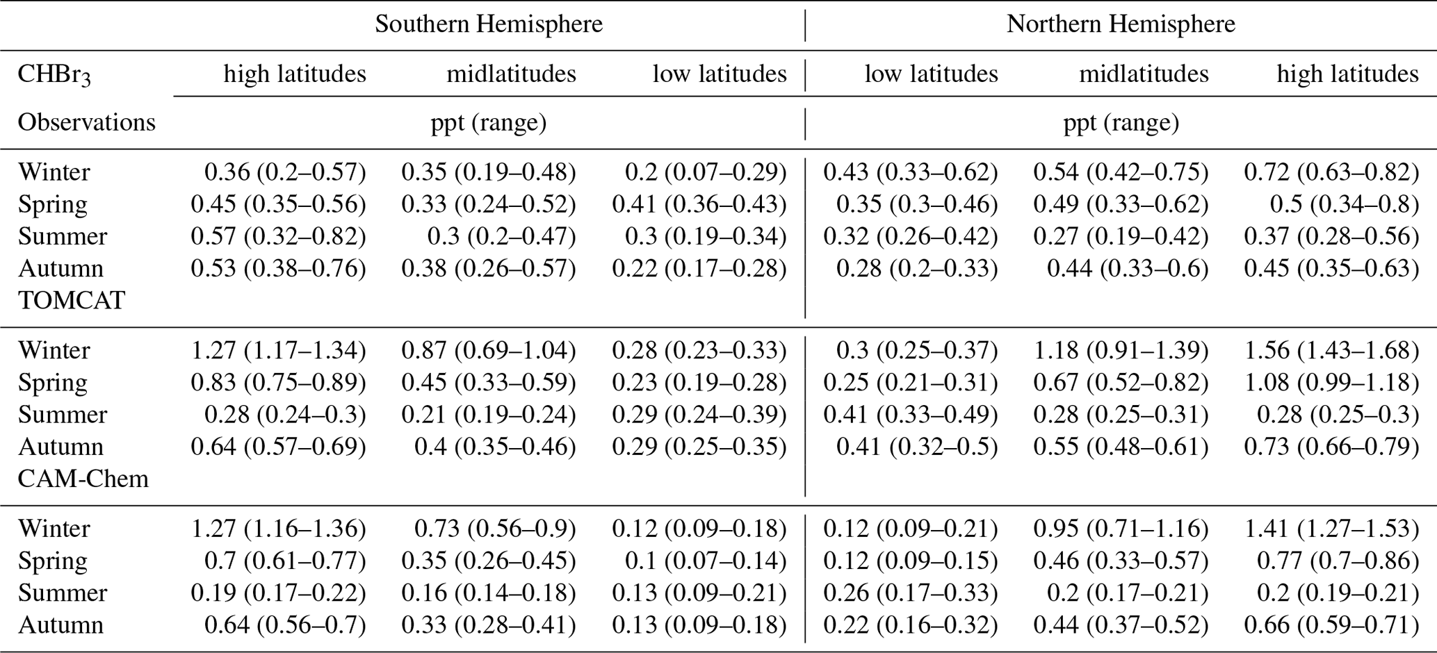

Figure 5Latitude cross section of tropopause representative mixing ratios of CH2Br2 from observation (black) and model results (blue for TOMCAT and green for CAM-Chem) for both hemispheres in winter. Data are binned into three latitude bins for each hemisphere: high latitudes (60–90∘), midlatitudes (30–60∘), and low latitudes (0–30∘) and only for data within the 10 K below the dynamical tropopause. Shown are the medians with the error bars representing the interquartile range (IQR). The median latitudinal position of observational and model bins may differ due to different spatial data coverage of observations and models. Also included is the reference mixing ratio for the tropical tropopause (Engel et al., 2018).
As shown in Table 1, low-latitude CH2Br2 values in both hemispheres during all seasons are well within the range reported by Engel et al. (2018) although with slightly higher mixing ratios. Keber et al. (2020) showed a clear tendency for an increase in tropopause mixing ratios with latitude in the NH, most pronounced in winter (see Fig. 5). This is likely due to the increase in lifetimes with latitude, as photochemical breakdown becomes slower with higher latitudes especially during winter. Our extended data set confirms the findings of Keber et al. (2020). In addition, we show that the SH upper-tropospheric distribution looks similar to that of the NH. Mixing ratios in NH winter and spring are slightly larger than in SH winter and spring, whereas mixing ratios in the respective hemispheric summer are close to each other across all latitudes. Larger differences are observed in the low and midlatitudes of NH and SH during autumn, with larger values in the NH than in the SH. However, the high latitudes of each autumn differ only to a small extent.
Both models qualitatively reproduce the larger CH2Br2 values in hemispheric winter and spring and smaller values in summer and autumn at high and midlatitudes (see Fig. S3 in the Supplement). However, both models overestimate low-latitude values for all seasons except for SH spring and NH winter. This overestimation in TOMCAT could already be seen in Keber et al. (2020) for the NH low latitudes for both winter and late summer to early autumn, as well as in Hossaini et al. (2013) where the TOMCAT model was only compared with HIPPO data. In general, CAM-Chem values are slightly smaller than TOMCAT values except in SH summer and autumn high latitudes. In NH winter, the models are close to observations (observations in between the model results), but both models overestimate NH spring values. However, both models reproduce the observed increase in mixing ratios with latitude in NH winter and spring, with CAM-Chem showing slightly better agreement. The models simulate SH winter and spring well in the midlatitudes and high latitudes, with TOMCAT somewhat closer to the winter observations, but none of the models capture the observed latitudinal variations in winter. The largest values in the models are found at high latitudes in spring for both hemispheres where observations show the largest values in hemispheric winter high latitudes (see Table 1 for absolute values). Summer and autumn of both hemispheres are in better agreement with CAM-Chem, as TOMCAT deviates more from the observations. TOMCAT generally simulates smaller mixing ratios in the SH and larger mixing ratios in NH summer and autumn midlatitudes and high latitudes.
For CHBr3 (see Table 2 and Figs. S2 and S4 in the Supplement), the upper-tropospheric distribution is much more variable and shows a less clear seasonality, especially in the SH. NH low-latitude values are slightly higher with a maximum in winter of 0.43 (0.33–0.62) ppt and maximum value in SH spring of 0.41 (0.36–0.43) ppt. NH values show an increase in mixing ratios with latitude, most pronounced in winter and spring. In NH summer, mixing ratios drop from low latitudes to midlatitudes and increase towards high latitudes again. Thus, the NH upper-tropospheric distribution of CHBr3 does not show the behaviour described in Keber et al. (2020) with an increase towards midlatitudes and a decrease at higher latitudes. Keber et al. (2020) considered a combined data set for summer and early autumn, whereas in this analysis summer and autumn are considered separately. As the latitudinal distribution differs substantially in summer and autumn (see Table 2), the separate consideration of summer and autumn compared to the combined consideration as in Keber et al. (2020) can lead to differences in the interpretation of the observations. The behaviour of CHBr3, which can be seen in the NH summer, is also observed in the SH spring as well. All other seasons of the SH show an increase in mixing ratios with latitude but with the largest values in summer and autumn high latitudes with up to 0.57 (0.32–0.82) ppt in SH summer.
TOMCAT simulates an increase in mixing ratio with latitude for almost all seasons, with the largest values occurring in hemispheric winter. Only in hemispheric summer do values decrease from low latitudes to midlatitudes and then increase slightly in SH high latitudes and remain at the same level in the NH high latitudes. Mid- and high-latitude mixing ratios in the NH are highly overestimated in winter, spring, and to a smaller extent in autumn, a feature already observed in Fig. 3. In the SH, midlatitude mixing ratios are also overestimated in winter, spring, and autumn, which is also true for high-latitude spring and autumn. In contrast, the observed and modelled mixing ratios in the SH high latitudes in winter and summer show a different behaviour. In the observations, the high-latitude values are smallest in the winter and highest in the summer, which is a reversed behaviour of the model estimations (see Table 2 or Fig. S4). As the high-latitude observations are much more limited during these seasons (see Fig. 2 or Table S1 in the Supplement), we are careful about interpreting these differences and further observations are needed to verify these deviations from model results. CAM-Chem upper-tropospheric distributions are similar to TOMCAT distributions, although in general they show smaller values for all latitudes. Thus, CHBr3 mixing ratios from CAM-Chem are somewhat closer to the observation in NH winter, spring, and autumn midlatitudes to high latitudes and deviate slightly more in NH summer, compared to TOMCAT. In the SH, spring and autumn distributions from CAM-Chem are closer to observations compared to winter and summer distributions. Like for TOMCAT, the seasonal variation within the high latitudes show a different behaviour in comparison to the observations, with an even smaller value from CAM-Chem in SH summer high latitudes. Overall, the distribution of CHBr3 is highly variable, and both models simulate a similar latitudinal distribution, though with smaller values for CAM-Chem. The tug of war between rapid advective transport and local accumulation at the time of emission plays a decisive role. As already mentioned, Jia et al. (2019) showed that transport variations in the atmosphere itself produce a highly variable Br-VSLS distribution with elevated values not always reflecting strong localized sources.
4.4 Midlatitude UTLS vertical profiles
The observational coverage of the upper troposphere and especially the lower stratosphere is best in spring and autumn of the respective hemisphere. From the altitude–latitude cross sections (Sect. 4.1, Figs. 2 and 3), we already suspect larger differences in the LMS Br-VSLS distribution in hemispheric autumn than in hemispheric spring.
We thus took a closer look at the vertical profiles of CH2Br2 and CHBr3 in the midlatitudes of the SH and NH during these seasons. The observations from the different missions were seasonally combined and have been binned in 10 K intervals of potential temperature and potential temperature difference to the local tropopause. Only bins with at least five observations are considered. For the profile in the free troposphere, data were binned in potential temperature (Θ). Data binned in potential temperature difference to the local tropopause (ΔΘ) show larger variability in the free troposphere (e.g. Keber et al., 2020). ΔΘ coordinates are therefore not well suited for tropospheric data. As ΔΘ coordinates reduce the variability of the profile near the tropopause and within the lowermost stratosphere (e.g. Keber et al., 2020), the profile continued from 10 K below the local tropopause into the stratosphere in ΔΘ coordinates. The two vertical coordinates were combined by aligning 0 K of ΔΘ with the median tropopause in Θ, observed during the measurements. Profiles in Θ coordinates may extend beyond the median tropopause even if the observations are declared as tropospheric ones. Tropopause Θ of these observations is much larger and corresponds to a higher tropopause, indicating that these observations may be subtropical in origin. The mixing ratios are averaged over equivalent latitude* of 40–60∘ of the respective hemisphere using box-and-whisker plots for the binned data (see Figs. 6 and 7). Vertical gradients for spring and autumn profiles for both hemispheres from tropopause values up to 30 K above the local tropopause are summarized in Table 3.
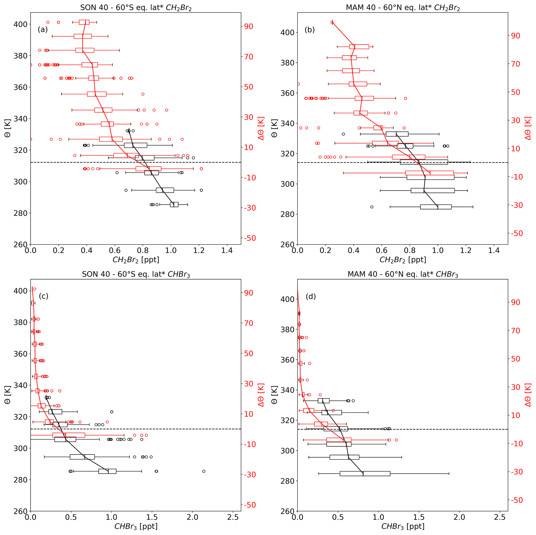
Figure 6Hemispheric spring vertical profiles of (a, b) CH2Br2 and (c, d) CHBr3. Observations were averaged over 40–60∘ of equivalent latitude*. Data are displayed as a function of potential temperature for tropospheric values (black) and potential temperature difference to the local tropopause for values from 10 K below the tropopause and above (red). Shown are the medians with the boxes representing the interquartile range (IQR), with whiskers as the 1.5×IQR, and circles are single observations outside the whiskers (outliers). The dashed black line shows the median dynamical tropopause derived from the times and locations of the observation.
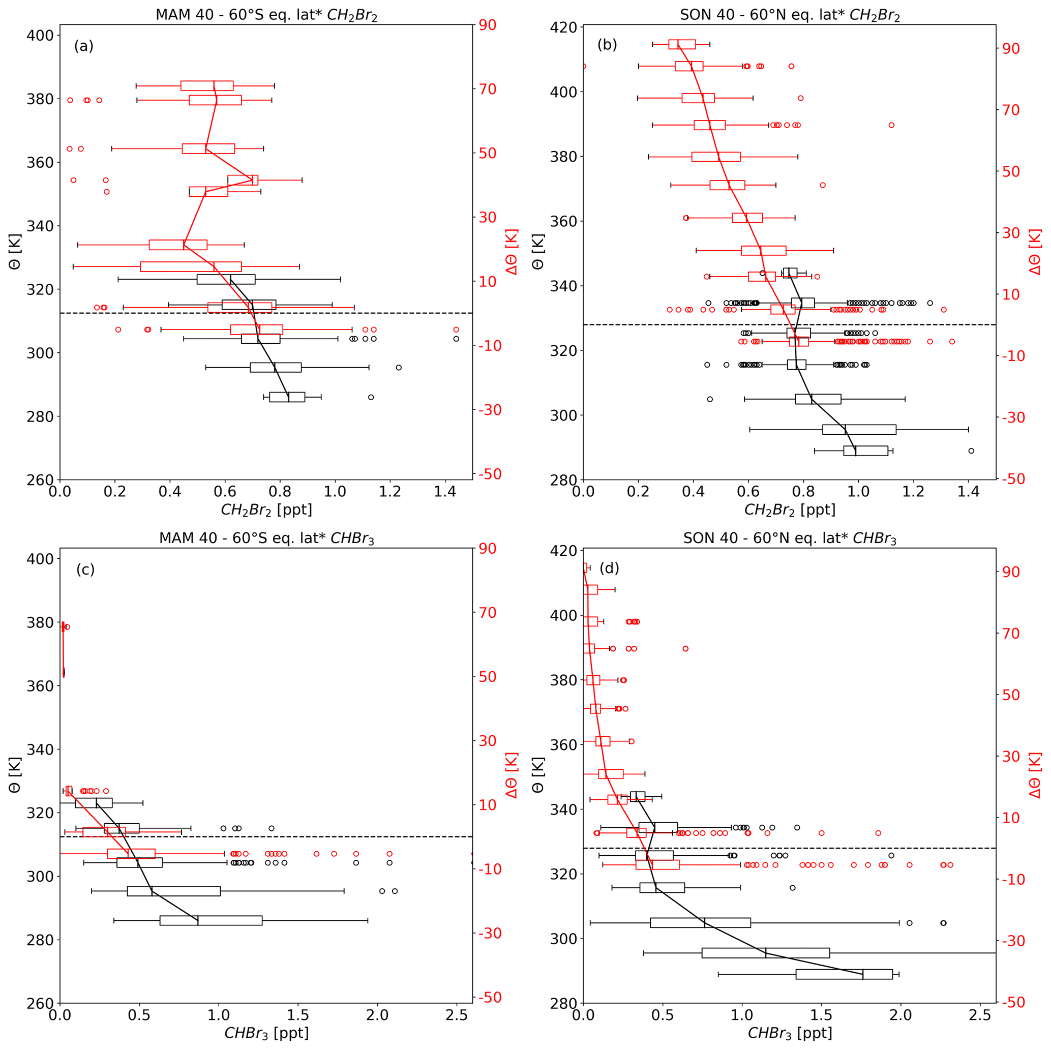
Table 3Vertical gradients across the tropopause in the Northern Hemisphere (NH) and Southern Hemisphere (SH) spring and autumn from tropopause (TP) mixing ratios from the 10 K bin below the dynamical tropopause up to the 20–30 K bin above the dynamical tropopause. In addition, local lifetimes of CH2Br2 and CHBr3 for the tropospheric tropics and northern hemispheric midlatitudes at 10 km, taken from Carpenter et al. (2014).
a Gradient from TP to 10–20 K.
Figure 6 shows hemispheric spring profiles of CH2Br2 and CHBr3. Upper-tropospheric values of CH2Br2 are very similar and close to 1 ppt in both hemispheres. The values at the tropopause are slightly larger (by 0.05–0.1 ppt) at the NH tropopause compared to the SH tropopause. The CH2Br2 profiles in the lowermost stratosphere of both hemispheres are very similar in their respective spring, beside an exceptional low value of 0.25 ppt at 90 K of ΔΘ in the NH. Vertical gradients of CHBr3 profiles are larger compared to CH2Br2, well in line with the much shorter lifetimes (see Table 3). Upper-tropospheric mixing ratios are slightly larger in SH midlatitudes (by roughly 0.16 ppt). However note that NH tropospheric values present a larger variability. In contrast, tropopause values are slightly larger in the NH than in the SH. Mixing ratios drop to values close to 0 in both hemispheres at about 30–40 K of Θ above the tropopause.
Figure 7 shows hemispheric autumn profiles of CH2Br2 and CHBr3 with less similarity between SH and NH profiles than in hemispheric spring for both compounds. Upper-tropospheric values of CH2Br2 are slightly larger in the NH with a difference of up to 0.16 ppt to the SH. Tropopause values for hemispheric autumn (Fig. 7a and b) are slightly smaller compared to hemispheric spring values (Fig. 6a and b), but hemispheric differences in spring and autumn are comparable. Differences between NH and SH autumn become larger on the lowest levels above the dynamical tropopause; i.e. in the ExTL. CH2Br2 shows a larger vertical gradient up to 30 K of ΔΘ in SH autumn than in NH autumn (see Table 3) reaching smallest value of 0.45 ppt between 20 and 30 K of ΔΘ. With a comparable distance to the dynamic tropopause, the value in the NH is 0.64 ppt. Between 40 and 70 K of ΔΘ, SH values range from 0.53 to 0.7 ppt associated with a large variability.
Figure 8 again shows the SH autumn vertical profile of CH2Br2, but two more profiles were included in ΔΘ coordinates with one profile excluding TOGA observations and one profile excluding WAS and PFP observations. The profile including only TOGA from ATom is much closer to the profile using all observations, whereas the profile including only WAS and PFP observations from ATom shows a much steeper gradient across the tropopause and much smaller values. The larger number of TOGA observations shifts the median towards larger values. The profile without TOGA measurements would be in line with the assumption of a strong transport barrier, e.g. the subtropical jet and exchange between stratosphere and troposphere only at the edges of the jets (e.g. Fig. 1 in Gettelman et al., 2011), while the profile without WAS and PFP shows a less strong but still larger transport barrier than in the NH autumn profile (Fig. 7b). The NH profile also shows a much smaller gradient compared to NH spring and less variability, which may indicate a well-mixed LMS. This is also well in line with finding by, e.g., Bönisch et al. (2009), who showed a flushing of the lowermost stratosphere in summer and autumn.
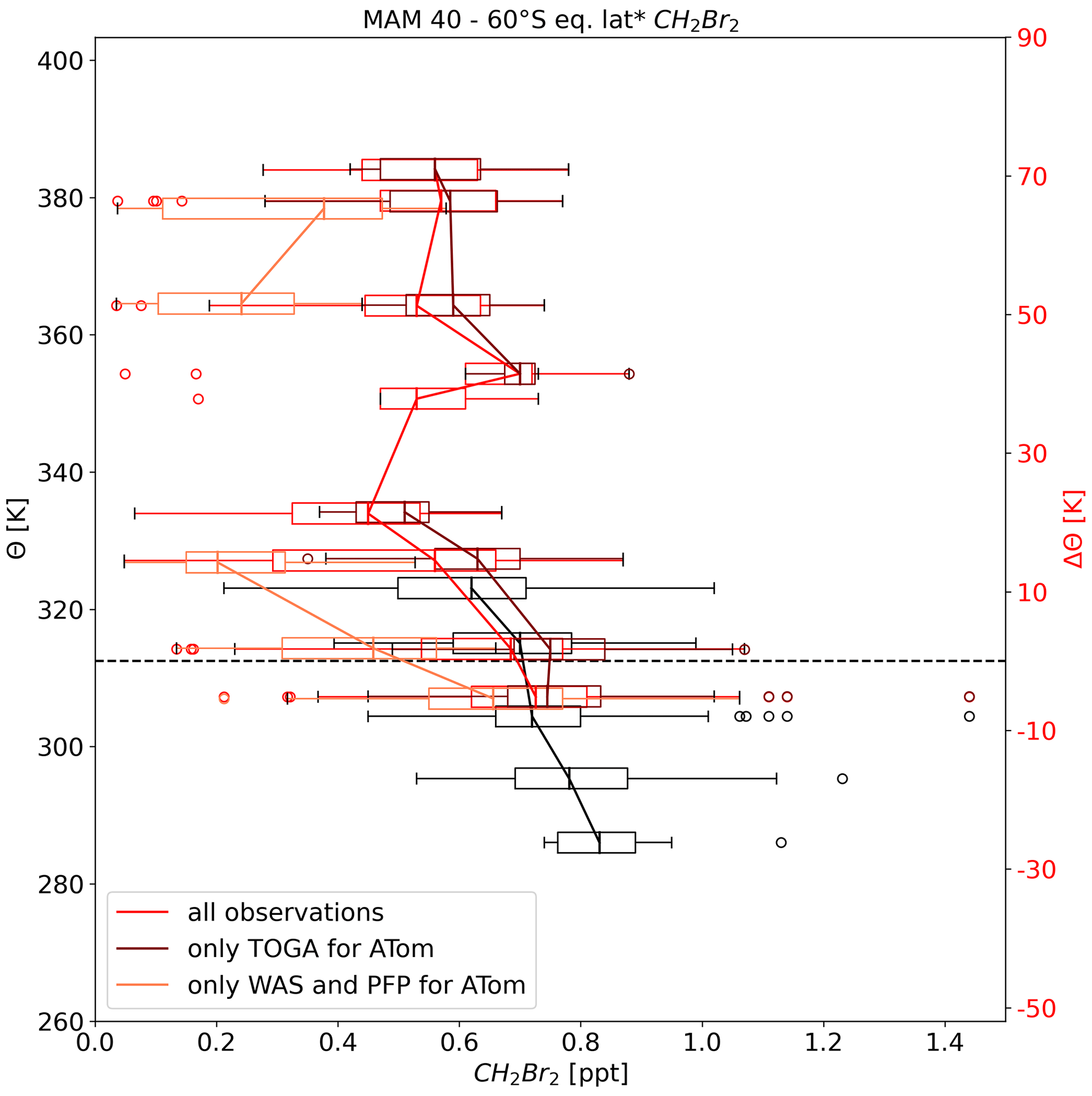
Figure 8As in Fig. 7 but only CH2Br2 for SH autumn. Profile as a function of potential temperature difference to the local tropopause was split into three profiles. Profile using all observations is in red, similar to Fig. 7, profile using all observation but with only TOGA observations from ATom in dark red, and profile using all observations but with only flask observations in light red.
Hemispherical differences can also be inferred from CHBr3 vertical profiles. Larger differences can be seen in the upper troposphere with nearly double the amount in the NH compared to the SH. In contrast, hemispheric differences at the tropopause are small (close to 0.5 ppt for both hemispheres). Regarding the LMS and especially the ExTL, the vertical gradient is much larger in the SH than in the NH. This implies that there is a stronger transport barrier in the SH when looking at CHBr3. SH values drop to almost 0 in the first 20 K above the dynamical tropopause but to around 0.22 ppt at a comparable distance to the NH autumn tropopause. Furthermore, NH lowermost-stratospheric values are steadily decreasing and are above 0.02 ppt even at 90 K of ΔΘ.
We further compared the midlatitude profiles of CH2Br2 and CHBr3 with model results of TOMCAT and CAM-Chem in Figs. 9 and 10. The comparisons are shown as a function of ΔΘ. Since there is no tropopause information for the TOMCAT model, we derived ΔΘ as the difference between the climatological tropopause potential temperature and model potential temperature. For consistency, the climatological tropopause was used for CAM-Chem as well. Additionally, since equivalent latitude information is not available for the models, latitude was used instead. The mean absolute percentage differences (MAPDs) reported below are tabled in the Supplement.

Figure 9Hemispheric spring vertical profiles of (a, b) CH2Br2 and (c, d) CHBr3. Observations were averaged over 40–60∘ of equivalent latitude*. Data are displayed as a function of potential temperature difference to the local tropopause (black). Also shown are model results from TOMCAT (blue) and CAM-Chem (green) as a function of potential temperature relative to the climatological tropopause. Profiles show medians with the boxes representing the interquartile range (IQR) and whiskers as the 1.5×IQR. Outliers are not included for a better illustration.
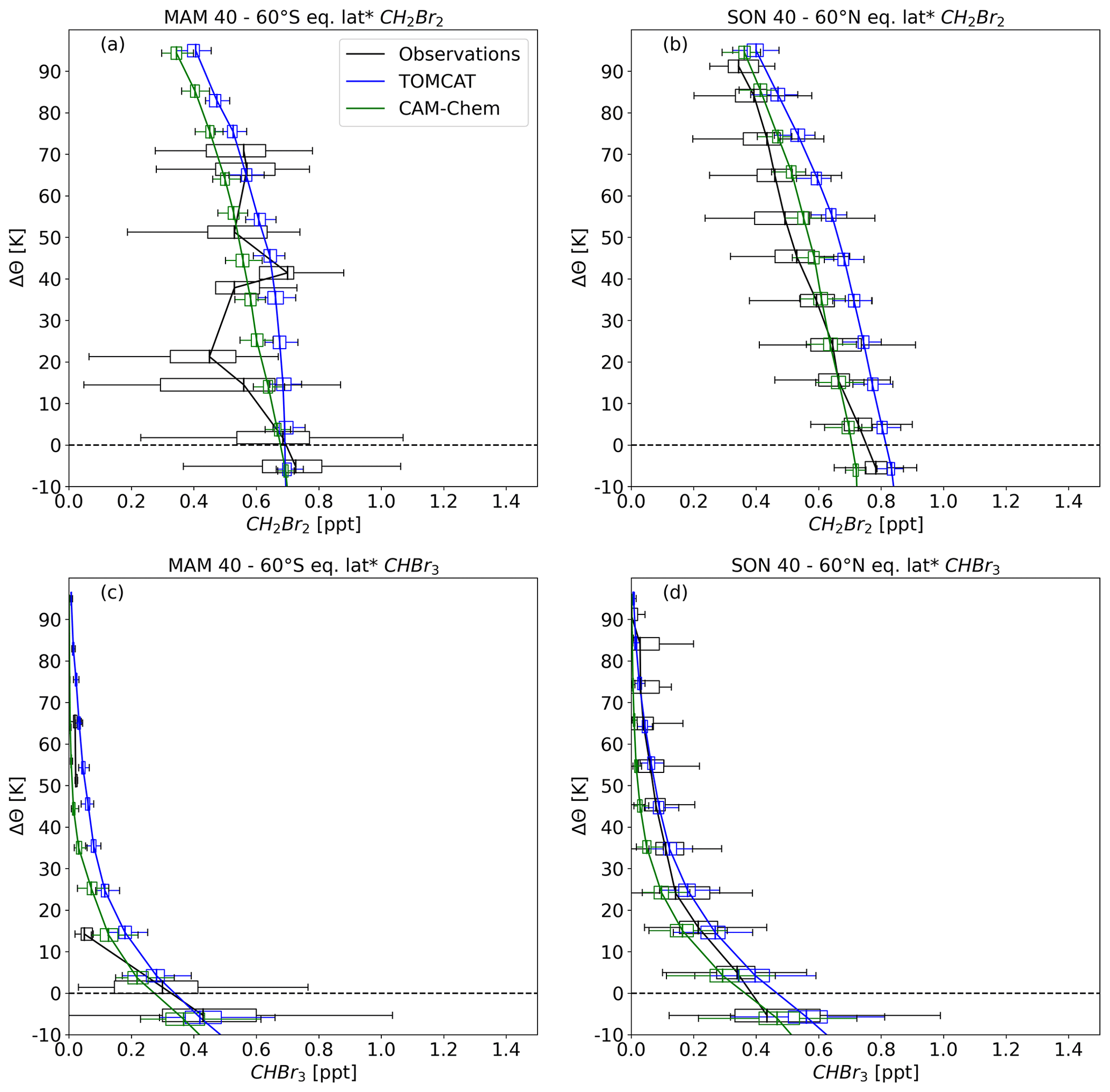
For spring CH2Br2 (Fig. 9a and b), TOMCAT profiles overestimate the observations on average by about 0.12 ppt in the NH and 0.08 ppt in the SH, with a corresponding MAPD of about 26 % (NH) and 18 % (SH). The CAM-Chem profiles are closer to the observations. Particularly the NH profile within the lowest 20 K above the dynamical tropopause is close to the observations but deviates towards higher altitudes. Average differences in the NH are 0.06 ppt and an MAPD of 17 %, whereas in the SH, differences are on average 0.03 ppt with an MAPD of 9 %. For CHBr3 (Fig. 9c and d), the comparison is only shown up to 40 K of ΔΘ, since this substance was almost completely depleted above. TOMCAT seems to overestimate NH CHBr3 by on average 0.1 ppt, corresponding to an MAPD of 69 %. Differences are much smaller in the SH with 0.02 ppt and an MAPD of 21 %. CAM-Chem estimated the lowermost stratosphere well in the NH with an average difference of 0.02 ppt and an MAPD of 15 %. SH differences in CAM-Chem are on average 0.04 ppt with an MAPD of 26 %, thus slightly larger than TOMCAT differences. Both models estimated a nearly complete depletion of CHBr3 in the SH lower stratosphere (above 40 K of ΔΘ). However, observations show a slight offset to the model estimations with values of 0.02–0.04 ppt up to 90 K of ΔΘ (Fig. 9c).
Hemispheric autumn midlatitude profiles of CH2Br2 and CHBr3 are displayed in Fig. 10. In NH autumn, the observed profiles and those of the models agree well. In the SH, however, the profiles diverge further as neither of the models reproduce the presumably stronger barrier at the tropopause described in Fig. 8. TOMCAT overestimates NH CH2Br2 up to 90 K of ΔΘ on average by about 0.1 ppt (MAPD of 20 %). The difference between models and observations becomes much larger in SH autumn. In addition, the observational profile exhibits a high degree of variability, and the scatter of the individual bins increases due to the differences between the ATom instruments, as mentioned earlier. Although models are close to observations above 40 K of ΔΘ, average differences between 0 and 40 K of ΔΘ are 0.12 ppt (MAPD of 25 %). CAM-Chem estimates are closer to the observations in the NH and differ on average by about 0.02 ppt corresponding to an MAPD of 6 %. However, CAM-Chem showed a similar profile to TOMCAT in the SH, although slightly smaller values in general and thus a smaller average difference between 0 and 40 K of ΔΘ of 0.06 ppt and an MAPD of 15 %. Compared to NH spring, TOMCAT shows a CHBr3 profile which is much closer to the observations in NH autumn. The average difference below 40 K of ΔΘ is 0.06 ppt with a corresponding MAPD of 22 %. SH observations are limited and thus a comparison is only possible up to 20 K of ΔΘ. Although observations and model results of TOMCAT are close near the dynamical tropopause, the difference increases rapidly to 0.13 ppt between 10 and 20 K of ΔΘ. As the CAM-Chem profile is smaller in absolute values, the largest differences are around 0.08 ppt. Both models fail to capture the steeper gradient across the dynamical tropopause during SH autumn.
In the present work, we investigated the global seasonal distribution of the two major short-lived brominated substances CH2Br2 and CHBr3. These natural substances with dominant oceanic origin gain importance because their relative contribution to the loss of ozone will rise as a result of the decline in the long-lived brominated substances of anthropogenic origin. We used data from four HALO missions: TACTS, WISE, PGS, and SouthTRAC. To further expand the data set, we included aircraft observations of the HIPPO and ATom missions. These are two global-scale missions, covering a wide latitude range in all seasons from the ground to the lowermost stratosphere. Zonal mean distributions were analysed by using latitude as the horizontal and pressure as the vertical coordinate (altitude–latitude cross sections). As the focus moved on to the tropopause region and lowermost stratosphere (upper-tropospheric distribution and vertical profiles), data are presented in potential temperature and further in a tropopause relative coordinate, namely the difference in potential temperature to the dynamical tropopause (ΔΘ). We further compared the observed distributions with two model distributions from TOMCAT and CAM-Chem, both using the Ordóñez et al. (2012) emission scenario, with emissions varying by season.
We found a similar tropospheric seasonality of CH2Br2 in both hemispheres, although with slightly larger mixing ratios in the NH. The larger values in the NH agree with expected hemispheric difference, as the main sources of many brominated VSLSs are believed to be stronger from coastal ocean regions. The ratio of ocean and land mass of the NH and SH is different, causing the size of coastal areas to vary. The upper-tropospheric distributions of CH2Br2 also show that the seasonality is similar in both hemispheres with larger values in winter and spring and smaller values in summer and autumn. In addition, in all seasons the mixing ratios are larger at NH midlatitudes and high latitudes than at the SH midlatitudes and high latitudes. Global seasonal distribution of CHBr3 shows larger variability and less clear seasonality. Although the NH mixing ratios seem to be larger in winter and spring than in summer and autumn, SH distributions show less seasonality with slightly larger values in autumn but overall smaller ones than in the NH. This may again be a result of the different ratio of ocean and land mass of both hemispheres. In good agreement with Keber et al. (2020), the mixing ratios at the extratropical tropopause are systematically larger than those at the tropical tropopause in both hemispheres at all times of the year. The comparison of the distributions in the UTLS was limited to hemispheric spring and autumn due to a lower coverage of the SH by observations. The LMS distributions in hemispheric spring are very similar (with differences well below 0.1 ppt) but differ considerably in hemispheric autumn (up to 0.3 ppt more in the NH). Midlatitude profiles of CH2Br2 and CHBr3, extending into the lowest stratosphere in hemispheric spring, are also similar, whereas profiles in hemispheric autumn differ much more. In particular, SH profiles of CH2Br2 and CHBr3 show much steeper gradients across the tropopause and into the stratosphere than NH profiles, and in the case of CH2Br2, SH observations present higher profile variability. This provides room for discussion as to whether the transport barrier in the SH autumn is significantly stronger, preventing the flushing of the lower stratosphere as it occurs in the NH summer and autumn. Unfortunately, in particular the observations in the lower stratosphere of the SH autumn show large differences between the different instruments on board the aircraft during ATom-4. Even if differences in the hemispheric autumn are already recognizable here, more observations and further investigation are needed to confirm an interhemispheric difference in the respective autumn lowermost stratosphere. The SH is less sampled than the NH and the observations may not be representative of the general distribution for all seasons in the SH.
We further compared the observed and modelled distributions from TOMCAT and CAM-Chem. The observed seasonality of CH2Br2 was only partially reproduced by the models and was not very pronounced in the SH, probably due to the emission scenario used, which for the high latitudes presents a homogeneous distribution and less pronounced seasonal cycle due to the scarcity of observations used in the construction of the scenario. The lack of aircraft observations in the SH led to issues regarding the emission flux estimates. In the case of CHBr3, both models systematically overestimate hemispheric winter and spring mixing ratios in the free troposphere and slightly underestimate hemispheric summer and autumn. In general, the mixing ratios in TOMCAT are larger than in CAM-Chem, which could be due to the differences in transport and the efficiency of the photochemical decomposition in the models when using the same emission scenario. Regarding upper-tropospheric distributions, the models reproduced the seasonality well with larger values in winter and spring and smaller values in summer and autumn. Model estimates are close to CH2Br2 observations for all seasons and both hemispheres, although the different flushing behaviour in the lower stratosphere between NH and SH is not captured by any of the models. Regarding CHBr3, both models yield significantly higher values in hemispheric winter midlatitudes and high latitudes than observed. The high-latitude observations of CHBr3 of the SH show a strong deviation from the models. Especially in winter and summer, the deviations are particularly large with observations showing reversed behaviour to the model simulations (largest values in summer and smallest values in winter). At these times of the year the flights do not reach such high latitudes (<70∘ S) and the number of observations in the high latitudes is very limited. For a more meaningful conclusion for the SH high latitudes, additional observations are needed. Modelled midlatitude vertical profiles agree well with observed profiles for NH spring and autumn as well as for SH spring. TOMCAT profiles are always slightly higher in mixing ratios than CAM-Chem and differences were therefore predominantly smaller when comparing with CAM-Chem. Both models were not capable of reproducing SH autumn vertical profiles of CH2Br2. Vertical gradients of CH2Br2 and CHBr3 across the tropopause in the respective autumn differ strongly from each other with steeper gradients in the SH autumn. Vertical gradients in the hemispheric spring, on the other hand, are more similar to each other.
Given these initial results of the global distribution of the two major Br-VSLSs, we reinforce the utility and need for further observations in the SH UTLS to further understand the seasonal distribution of theses species. Especially in the southern hemispheric UTLS, data coverage remains sparse in most seasons. First differences between the NH and SH could already be indicated based on the data used; thus extrapolating northern hemispheric observations to the SH is not possible. The representation of seasonal variability of Br-VSLS emissions and the efficiency of photochemical processes within the high latitudes need to be improved individually for the NH and SH to improve the agreement with current and future observations. In addition, it is of importance to generate a long-term global data set that can be used to determine if there is a trend in Br-VSLS abundance at the global and hemispheric scale.
Observational data from the HALO missions are available via the HALO Database (https://halo-db.pa.op.dlr.de/, last access: 22 June 2022). ATom observational data are available at the Oak Ridge National Laboratory Distributed Active Archive Center (ORNL DAAC; https://doi.org/10.3334/ORNLDAAC/1925; Wofsy et al., 2021). HIPPO observational data are available at the Earth Observing Laboratory data archive (EOL data archive, Wofsy et al., 2017). Model data are available on request: please contact Ryan Hossaini (r.hossaini@lancaster.ac.uk) for TOMCAT model data and Rafael P. Fernandez (rpfernandez@mendoza-conicet.gob.ar) for CAM-Chem model data.
The supplement related to this article is available online at: https://doi.org/10.5194/acp-22-15049-2022-supplement.
MJ, TK, TS, TW, and AE were involved in developing and operating the GhOST instrument. ELA and SM operated the instruments during HIPPO, and ECA, RSH, SM, and DRB operated the instruments during ATom. RH, RPF, ASL, and JUG provided model data and participated in the discussion regarding model comparison. MJ wrote the article with involvement of AE and TS in the analysis and writing process. All co-authors were involved in the discussion and iteration process of the article.
At least one of the (co-)authors is a member of the editorial board of Atmospheric Chemistry and Physics. The peer-review process was guided by an independent editor, and the authors also have no other competing interests to declare.
Publisher's note: Copernicus Publications remains neutral with regard to jurisdictional claims in published maps and institutional affiliations.
Dough Kinnison is thanked for helping with the high-resolution SD-CAM-Chem setup.
This research has been supported by the Bundesministerium für Bildung und Forschung (grant no. 01LG1908B), the Deutsche Forschungsgemeinschaft (grant nos. EN367/13-1, EN367/14-1, EN367/16-1, EN367/17-1), and DFG collaborative research program “The Tropopause Region in an Changing Atmosphere” TRR 301 – Project-ID 428312742, the National Center for Atmospheric Research (grant no. 1852977), the Consejo Nacional de Investigaciones Científicas y Técnicas (grant no. PICT 2019-2187), and the Natural Environment Research Council (grant no. NE/N014375/).
This open-access publication was funded by the Goethe University Frankfurt.
This paper was edited by Aurélien Dommergue and reviewed by two anonymous referees.
Abrahamsson, K., Granfors, A., Ahnoff, M., Cuevas, C. A., and Saiz-Lopez, A.: Organic bromine compounds produced in sea ice in Antarctic winter, Nat. Commun., 9, 5291, https://doi.org/10.1038/s41467-018-07062-8, 2018. a, b
Apel, E. C., Hornbrook, R. S., Hills, A. J., Blake, N. J., Barth, M. C., Weinheimer, A., Cantrell, C., Rutledge, S. A., Basarab, B., Crawford, J., Diskin, G., Homeyer, C. R., Campos, T., Flocke, F., Fried, A., Blake, D. R., Brune, W., Pollack, I., Peischl, J., Ryerson, T., Wennberg, P. O., Crounse, J. D., Wisthaler, A., Mikoviny, T., Huey, G., Heikes, B., O'Sullivan, D., and Riemer, D. D.: Upper tropospheric ozone production from lightning NOx-impacted convection: Smoke ingestion case study from the DC3 campaign, J. Geophys. Res.-Atmos., 120, 2505–2523, https://doi.org/10.1002/2014jd022121, 2015. a
Asher, E., Hornbrook, R. S., Stephens, B. B., Kinnison, D., Morgan, E. J., Keeling, R. F., Atlas, E. L., Schauffler, S. M., Tilmes, S., Kort, E. A., Hoecker-Martínez, M. S., Long, M. C., Lamarque, J.-F., Saiz-Lopez, A., McKain, K., Sweeney, C., Hills, A. J., and Apel, E. C.: Novel approaches to improve estimates of short-lived halocarbon emissions during summer from the Southern Ocean using airborne observations, Atmos. Chem. Phys., 19, 14071–14090, https://doi.org/10.5194/acp-19-14071-2019, 2019. a, b
Atlas, E.: Advanced Whole Air Sampler (AWAS) for HIAPER, UCAR/NCAR – Earth Observing Laboratory, https://doi.org/10.5065/D65X270F, 2016. a
Barletta, B., Biggs, B., Blake, D., Blake, N., Hoffman, A., Hughes, S., Meinardi, S., Vieznor, N., and Woods, C.: ATom: L2 Halocarbons and Hydrocarbons from the UC-Irvine Whole Air Sampler (WAS), https://doi.org/10.3334/ORNLDAAC/1751, 2019. a
Birner, T. and Bönisch, H.: Residual circulation trajectories and transit times into the extratropical lowermost stratosphere, Atmos. Chem. Phys., 11, 817–827, https://doi.org/10.5194/acp-11-817-2011, 2011. a
Bönisch, H., Engel, A., Curtius, J., Birner, Th., and Hoor, P.: Quantifying transport into the lowermost stratosphere using simultaneous in-situ measurements of SF6 and CO2, Atmos. Chem. Phys., 9, 5905–5919, https://doi.org/10.5194/acp-9-5905-2009, 2009. a, b, c, d
Boudjellaba, D., Dron, J., Revenko, G., Demelas, C., and Boudenne, J.-E.: Chlorination by-product concentration levels in seawater and fish of an industrialised bay (Gulf of Fos, France) exposed to multiple chlorinated effluents, Sci. Total Environ., 541, 391–399, https://doi.org/10.1016/j.scitotenv.2015.09.046, 2016. a
Butchart, N. and Remsberg, E. E.: The Area of the Stratospheric Polar Vortex as a Diagnostic for Tracer Transport on an Isentropic Surface, J. Atmos. Sci., 43, 1319–1339, https://doi.org/10.1175/1520-0469(1986)043<1319:TAOTSP>2.0.CO;2, 1986. a
Carpenter, L. J. and Liss, P. S.: On temperate sources of bromoform and other reactive organic bromine gases, J. Geophys. Res.-Atmos., 105, 20539–20547, https://doi.org/10.1029/2000jd900242, 2000. a
Carpenter, L. J., Wevill, D. J., O'Doherty, S., Spain, G., and Simmonds, P. G.: Atmospheric bromoform at Mace Head, Ireland: seasonality and evidence for a peatland source, Atmos. Chem. Phys., 5, 2927–2934, https://doi.org/10.5194/acp-5-2927-2005, 2005. a
Carpenter, L. J., Reimann, S., Burkholder, J. B., Clerbaux, C., Hall, B. D., Hossaini, R., Laube, J. C., and Yvon-Lewis, S. A.: Ozone-Depleting Substances (ODSs) and Other Gases of Interest to the Montreal Protocol, Chap. 1, World Meteorological Organization, Geneva, Switzerland, 55, ISBN 978-9966-076-01-4, 2014. a
Chipperfield, M. P.: New version of the TOMCAT/SLIMCAT off-line chemical transport model: Intercomparison of stratospheric tracer experiments, Q. J. Roy. Meteor. Soc., 132, 1179–1203, https://doi.org/10.1256/qj.05.51, 2006. a
Daniel, J. S., Solomon, S., and Portmann, R. W.: Stratospheric ozone depletion: The importance of bromine relative to chlorine, J. Geophys. Res.-Atmos., 104, 23871–23880, https://doi.org/10.1029/1999JD900381, 1999. a
Dee, D. P., Uppala, S. M., Simmons, A. J., Berrisford, P., Poli, P., Kobayashi, S., Andrae, U., Balmaseda, M. A., Balsamo, G., Bauer, P., Bechtold, P., Beljaars, A. C. M., van de Berg, L., Bidlot, J., Bormann, N., Delsol, C., Dragani, R., Fuentes, M., Geer, A. J., Haimberger, L., Healy, S. B., Hersbach, H., Hòlm, E. V., Isaksen, L., Kållberg, P., Köhler, M., Matricardi, M., McNally, A. P., Monge-Sanz, B. M., Morcrette, J.-J., Park, B.-K., Peubey, C., de Rosnay, P., Tavalato, C., Thépaut, J.-N., and Vitart, F.: The ERA-Interim reanalysis: Configuration and performance of the data assimilation system, Q. J. Roy. Meteor. Soc., 137, 553–597, https://doi.org/10.1002/qj.828, 2011. a
Engel, A., Rigby, M., Burkholder, J. B., Fernandez, R. P., Froidevaux, L., Hall, B. D., Hossaini, R., Saito, T., Vollmer, M. K., and Yao, B.: Update on Ozone-Depletion Substances (ODSs) and other Gases of Interest to the Montreal Protocol, Chap. 1, World Meteorological Organization, Geneva, Switzerland, 58, ISBN 978-1-7329317-1-8, 2018. a, b, c, d, e, f
Fernandez, R. P., Salawitch, R. J., Kinnison, D. E., Lamarque, J.-F., and Saiz-Lopez, A.: Bromine partitioning in the tropical tropopause layer: implications for stratospheric injection, Atmos. Chem. Phys., 14, 13391–13410, https://doi.org/10.5194/acp-14-13391-2014, 2014. a
Fernandez, R. P., Kinnison, D. E., Lamarque, J.-F., Tilmes, S., and Saiz-Lopez, A.: Impact of biogenic very short-lived bromine on the Antarctic ozone hole during the 21st century, Atmos. Chem. Phys., 17, 1673–1688, https://doi.org/10.5194/acp-17-1673-2017, 2017. a
Gettelman, A., Hoor, P., Pan, L. L., Randel, W. J., Hegglin, M. I., and Birner, T.: The extratropical upper troposphere and lower stratosphere, Rev. Geophys., 49, https://doi.org/10.1029/2011RG000355, 2011. a, b, c
Grooß, J.-U., Engel, I., Borrmann, S., Frey, W., Günther, G., Hoyle, C. R., Kivi, R., Luo, B. P., Molleker, S., Peter, T., Pitts, M. C., Schlager, H., Stiller, G., Vömel, H., Walker, K. A., and Müller, R.: Nitric acid trihydrate nucleation and denitrification in the Arctic stratosphere, Atmos. Chem. Phys., 14, 1055–1073, https://doi.org/10.5194/acp-14-1055-2014, 2014. a
Hamed, M. A., Moustafa, M. E., Soliman, Y. A., El-Sawy, M. A., and Khedr, A. I.: Trihalomethanes formation in marine environment in front of Nuweibaa desalination plant as a result of effluents loaded by chlorine residual, The Egyptian Journal of Aquatic Research, 43, 45–54, https://doi.org/10.1016/j.ejar.2017.01.001, 2017. a
Hegglin, M. I. and Shepherd, T. G.: O3–N2O correlations from the Atmospheric Chemistry Experiment: Revisiting a diagnostic of transport and chemistry in the stratosphere, J. Geophys. Res.-Atmos., 112, https://doi.org/10.1029/2006jd008281, 2007. a
Hegglin, M. I., Boone, C. D., Manney, G. L., and Walker, K. A.: A global view of the extratropical tropopause transition layer from Atmospheric Chemistry Experiment Fourier Transform Spectrometer O3, H2O, and CO, J. Geophys. Res.-Atmos., 114, https://doi.org/10.1029/2008JD009984, 2009. a, b
Hersbach, H., Bell, B., Berrisford, P., Hirahara, S., Horányi, A., Muñoz-Sabater, J., Nicolas, J., Peubey, C., Radu, R., Schepers, D., Simmons, A., Soci, C., Abdalla, S., Abellan, X., Balsamo, G., Bechtold, P., Biavati, G., Bidlot, J., Bonavita, M., De Chiara, G., Dahlgren, P., Dee, D., Diamantakis, M., Dragani, R., Flemming, J., Forbes, R., Fuentes, M., Geer, A., Haimberger, L., Healy, S., Hogan, R. J., Hólm, E., Janisková, M., Keeley, S., Laloyaux, P., Lopez, P., Lupu, C., Radnoti, G., de Rosnay, P., Rozum, I., Vamborg, F., Villaume, S., and Thépaut, J.-N.: The ERA5 global reanalysis, Q. J. Roy. Meteor. Soc., 146, 1999–2049, https://doi.org/10.1002/qj.3803, 2020. a
Hoor, P., Fischer, H., and Lelieveld, J.: Tropical and extratropical tropospheric air in the lowermost stratosphere over Europe: A CO-based budget, Geophys. Res. Lett., 32, L07802, https://doi.org/10.1029/2004GL022018, 2005. a, b, c
Hossaini, R., Mantle, H., Chipperfield, M. P., Montzka, S. A., Hamer, P., Ziska, F., Quack, B., Krüger, K., Tegtmeier, S., Atlas, E., Sala, S., Engel, A., Bönisch, H., Keber, T., Oram, D., Mills, G., Ordóñez, C., Saiz-Lopez, A., Warwick, N., Liang, Q., Feng, W., Moore, F., Miller, B. R., Marécal, V., Richards, N. A. D., Dorf, M., and Pfeilsticker, K.: Evaluating global emission inventories of biogenic bromocarbons, Atmos. Chem. Phys., 13, 11819–11838, https://doi.org/10.5194/acp-13-11819-2013, 2013. a, b
Hossaini, R., Chipperfield, M. P., Montzka, S. A., Rap, A., Dhomse, S., and Feng, W.: Efficiency of short-lived halogens at influencing climate through depletion of stratospheric ozone, Nat. Geosci., 8, 1427–1442, https://doi.org/10.1038/ngeo2363, 2015. a
Hossaini, R., Patra, P. K., Leeson, A. A., Krysztofiak, G., Abraham, N. L., Andrews, S. J., Archibald, A. T., Aschmann, J., Atlas, E. L., Belikov, D. A., Bönisch, H., Carpenter, L. J., Dhomse, S., Dorf, M., Engel, A., Feng, W., Fuhlbrügge, S., Griffiths, P. T., Harris, N. R. P., Hommel, R., Keber, T., Krüger, K., Lennartz, S. T., Maksyutov, S., Mantle, H., Mills, G. P., Miller, B., Montzka, S. A., Moore, F., Navarro, M. A., Oram, D. E., Pfeilsticker, K., Pyle, J. A., Quack, B., Robinson, A. D., Saikawa, E., Saiz-Lopez, A., Sala, S., Sinnhuber, B.-M., Taguchi, S., Tegtmeier, S., Lidster, R. T., Wilson, C., and Ziska, F.: A multi-model intercomparison of halogenated very short-lived substances (TransCom-VSLS): linking oceanic emissions and tropospheric transport for a reconciled estimate of the stratospheric source gas injection of bromine, Atmos. Chem. Phys., 16, 9163–9187, https://doi.org/10.5194/acp-16-9163-2016, 2016. a, b, c, d, e, f, g
Jesswein, M., Bozem, H., Lachnitt, H.-C., Hoor, P., Wagenhäuser, T., Keber, T., Schuck, T., and Engel, A.: Comparison of inorganic chlorine in the Antarctic and Arctic lowermost stratosphere by separate late winter aircraft measurements, Atmos. Chem. Phys., 21, 17225–17241, https://doi.org/10.5194/acp-21-17225-2021, 2021. a, b, c
Jia, Y., Tegtmeier, S., Atlas, E., and Quack, B.: How marine emissions of bromoform impact the remote atmosphere, Atmos. Chem. Phys., 19, 11089–11103, https://doi.org/10.5194/acp-19-11089-2019, 2019. a, b
Keber, T., Bönisch, H., Hartick, C., Hauck, M., Lefrancois, F., Obersteiner, F., Ringsdorf, A., Schohl, N., Schuck, T., Hossaini, R., Graf, P., Jöckel, P., and Engel, A.: Bromine from short-lived source gases in the extratropical northern hemispheric upper troposphere and lower stratosphere (UTLS), Atmos. Chem. Phys., 20, 4105–4132, https://doi.org/10.5194/acp-20-4105-2020, 2020. a, b, c, d, e, f, g, h, i, j, k, l, m, n, o, p, q, r, s
Klobas, J. E., Weisenstein, D. K., Salawitch, R. J., and Wilmouth, D. M.: Reformulating the bromine alpha factor and equivalent effective stratospheric chlorine (EESC): evolution of ozone destruction rates of bromine and chlorine in future climate scenarios, Atmos. Chem. Phys., 20, 9459–9471, https://doi.org/10.5194/acp-20-9459-2020, 2020. a
Konopka, P., Ploeger, F., Tao, M., Birner, T., and Riese, M.: Hemispheric asymmetries and seasonality of mean age of air in the lower stratosphere: Deep versus shallow branch of the Brewer–Dobson circulation, J. Geophys. Res.-Atmos., 120, 2053–2066, https://doi.org/10.1002/2014jd022429, 2015. a, b
Kunkel, D., Hoor, P., Kaluza, T., Ungermann, J., Kluschat, B., Giez, A., Lachnitt, H.-C., Kaufmann, M., and Riese, M.: Evidence of small-scale quasi-isentropic mixing in ridges of extratropical baroclinic waves, Atmos. Chem. Phys., 19, 12607–12630, https://doi.org/10.5194/acp-19-12607-2019, 2019. a, b
Lamarque, J.-F., Emmons, L. K., Hess, P. G., Kinnison, D. E., Tilmes, S., Vitt, F., Heald, C. L., Holland, E. A., Lauritzen, P. H., Neu, J., Orlando, J. J., Rasch, P. J., and Tyndall, G. K.: CAM-chem: description and evaluation of interactive atmospheric chemistry in the Community Earth System Model, Geosci. Model Dev., 5, 369–411, https://doi.org/10.5194/gmd-5-369-2012, 2012. a
Leedham, E. C., Hughes, C., Keng, F. S. L., Phang, S.-M., Malin, G., and Sturges, W. T.: Emission of atmospherically significant halocarbons by naturally occurring and farmed tropical macroalgae, Biogeosciences, 10, 3615–3633, https://doi.org/10.5194/bg-10-3615-2013, 2013. a
Liu, Y., Yvon-Lewis, S., Hu, L., Salisbury, J., and O'Hern, J.: CHBr3, CH2Br2, and CHClBr2 in the U. S. coastal waters during the Gulf of Mexico and East Coast Carbon cruise, J. Geophys. Res.-Oceans, 116, https://doi.org/10.1029/2010JC006729, 2011. a
Maas, J., Tegtmeier, S., Quack, B., Biastoch, A., Durgadoo, J. V., Rühs, S., Gollasch, S., and David, M.: Simulating the spread of disinfection by-products and anthropogenic bromoform emissions from ballast water discharge in Southeast Asia, Ocean Sci., 15, 891–904, https://doi.org/10.5194/os-15-891-2019, 2019. a
Maas, J., Tegtmeier, S., Jia, Y., Quack, B., Durgadoo, J. V., and Biastoch, A.: Simulations of anthropogenic bromoform indicate high emissions at the coast of East Asia, Atmos. Chem. Phys., 21, 4103–4121, https://doi.org/10.5194/acp-21-4103-2021, 2021. a
Monks, S. A., Arnold, S. R., Hollaway, M. J., Pope, R. J., Wilson, C., Feng, W., Emmerson, K. M., Kerridge, B. J., Latter, B. L., Miles, G. M., Siddans, R., and Chipperfield, M. P.: The TOMCAT global chemical transport model v1.6: description of chemical mechanism and model evaluation, Geosci. Model Dev., 10, 3025–3057, https://doi.org/10.5194/gmd-10-3025-2017, 2017. a
Navarro, M. A., Atlas, E. L., Saiz-Lopez, A., Rodriguez-Lloveras, X., Kinnison, D. E., Lamarque, J.-F., Tilmes, S., Filus, M., Harris, N. R. P., Meneguz, E., Ashfold, M. J., Manning, A. J., Cuevas, C. A., Schauffler, S. M., and Donets, V.: Airborne measurements of organic bromine compounds in the Pacific tropical tropopause layer, P. Natl. Acad. Sci. USA, 112, 13789–13793, https://doi.org/10.1073/pnas.1511463112, 2015. a, b
Oelhaf, H., Sinnhuber, B.-M., Woiwode, W., Bönisch, H., Bozem, H., Engel, A., Fix, A., Friedl-Vallon, F., Grooß, J.-U., Hoor, P., Johansson, S., Jurkat-Witschas, T., Kaufmann, S., Krämer, M., Krause, J., Kretschmer, E., Lörks, D., Marsing, A., Orphal, J., Pfeilsticker, K., Pitts, M., Poole, L., Preusse, P., Rapp, M., Riese, M., Rolf, C., Ungermann, J., Voigt, C., Volk, C. M., Wirth, M., Zahn, A., and Ziereis, H.: POLSTRACC: Airborne Experiment for Studying the Polar Stratosphere in a Changing Climate with the High Altitude and Long Range Research Aircraft (HALO), B. Am. Meteorol. Soc., 100, 2634–2664, https://doi.org/10.1175/BAMS-D-18-0181.1, 2019. a
Ordóñez, C., Lamarque, J.-F., Tilmes, S., Kinnison, D. E., Atlas, E. L., Blake, D. R., Sousa Santos, G., Brasseur, G., and Saiz-Lopez, A.: Bromine and iodine chemistry in a global chemistry-climate model: description and evaluation of very short-lived oceanic sources, Atmos. Chem. Phys., 12, 1423–1447, https://doi.org/10.5194/acp-12-1423-2012, 2012. a, b, c, d, e, f, g, h, i, j, k
Pan, L. L., Kunz, A., Homeyer, C. R., Munchak, L. A., Kinnison, D. E., and Tilmes, S.: Commentary on using equivalent latitude in the upper troposphere and lower stratosphere, Atmos. Chem. Phys., 12, 9187–9199, https://doi.org/10.5194/acp-12-9187-2012, 2012. a
Pan, L. L., Atlas, E. L., Salawitch, R. J., Honomichl, S. B., Bresch, J. F., Randel, W. J., Apel, E. C., Hornbrook, R. S., Weinheimer, A. J., Anderson, D. C., Andrews, S. J., Baidar, S., Beaton, S. P., Campos, T. L., Carpenter, L. J., Chen, D., Dix, B., Donets, V., Hall, S. R., Hanisco, T. F., Homeyer, C. R., Huey, L. G., Jensen, J. B., Kaser, L., Kinnison, D. E., Koenig, T. K., Lamarque, J.-F., Liu, C., Luo, J., Luo, Z. J., Montzka, D. D., Nicely, J. M., Pierce, R. B., Riemer, D. D., Robinson, T., Romashkin, P., Saiz-Lopez, A., Schauffler, S., Shieh, O., Stell, M. H., Ullmann, K., Vaughan, G., Volkamer, R., and Wolfe, G.: The Convective Transport of Active Species in the Tropics (CONTRAST) Experiment, B. Am. Meteorol. Soc., 98, 106–128, https://doi.org/10.1175/BAMS-D-14-00272.1, 2017. a
Patra, P. K., Houweling, S., Krol, M., Bousquet, P., Belikov, D., Bergmann, D., Bian, H., Cameron-Smith, P., Chipperfield, M. P., Corbin, K., Fortems-Cheiney, A., Fraser, A., Gloor, E., Hess, P., Ito, A., Kawa, S. R., Law, R. M., Loh, Z., Maksyutov, S., Meng, L., Palmer, P. I., Prinn, R. G., Rigby, M., Saito, R., and Wilson, C.: TransCom model simulations of CH4 and related species: linking transport, surface flux and chemical loss with CH4 variability in the troposphere and lower stratosphere, Atmos. Chem. Phys., 11, 12813–12837, https://doi.org/10.5194/acp-11-12813-2011, 2011. a
Quack, B., Peeken, I., Petrick, G., and Nachtigall, K.: Oceanic distribution and sources of bromoform and dibromomethane in the Mauritanian upwelling, J. Geophys. Res.-Oceans, 112, 1–13, https://doi.org/10.1029/2006JC003803, 2007. a
Quivet, E., Höhener, P., Temime-Roussel, B., Dron, J., Revenko, G., Verlande, M., Lebaron, K., Demelas, C., Vassalo, L., and Boudenne, J.-L.: Underestimation of Anthropogenic Bromoform Released into the Environment?, Environ. Sci. Technol., 56, 1522–1533, https://doi.org/10.1021/acs.est.1c05073, 2022. a, b
Sala, S., Bönisch, H., Keber, T., Oram, D. E., Mills, G., and Engel, A.: Deriving an atmospheric budget of total organic bromine using airborne in situ measurements from the western Pacific area during SHIVA, Atmos. Chem. Phys., 14, 6903–6923, https://doi.org/10.5194/acp-14-6903-2014, 2014. a
Salawitch, R. J., Weisenstein, D. K., Kovalenko, L. J., Sioris, C. E., Wennberg, P. O., Chance, K., Ko, M. K. W., and McLinden, C. A.: Sensitivity of ozone to bromine in the lower stratosphere, Geophys. Res. Lett., 32, 1–5, https://doi.org/10.1029/2004GL021504, 2005. a
Sam Yang, J.: Bromoform in the effluents of a nuclear power plant: a potential tracer of coastal water masses, Hydrobiologia, 464, 99–105, https://doi.org/10.1023/A:1013922731434, 2001. a
Shuckburgh, E., d'Ovidio, F., and Legras, B.: Local Mixing Events in the Upper Troposphere and Lower Stratosphere. Part II: Seasonal and Interannual Variability, J. Atmos. Sci., 66, 3695–3706, https://doi.org/10.1175/2009JAS2983.1, 2009. a
Sinnhuber, B.-M., Sheode, N., Sinnhuber, M., Chipperfield, M. P., and Feng, W.: The contribution of anthropogenic bromine emissions to past stratospheric ozone trends: a modelling study, Atmos. Chem. Phys., 9, 2863–2871, https://doi.org/10.5194/acp-9-2863-2009, 2009. a
Sturges, W. T., Sullivan, C. W., Schnell, R. C., Heidt, L. E., and Pollock, W. H.: Bromoalkane production by Antarctic ice algae, Tellus B, 45, 120–126, https://doi.org/10.3402/tellusb.v45i2.15586, 1993. a
Tegtmeier, S., Atlas, E., Quack, B., Ziska, F., and Krüger, K.: Variability and past long-term changes of brominated very short-lived substances at the tropical tropopause, Atmos. Chem. Phys., 20, 7103–7123, https://doi.org/10.5194/acp-20-7103-2020, 2020. a
Thompson, C. R., Wofsy, S. C., Prather, M. J., Newman, P. A., Hanisco, T. F., Ryerson, T. B., Fahey, D. W., Apel, E. C., Brock, C. A., Brune, W. H., Froyd, K., Katich, J. M., Nicely, J. M., Peischl, J., Ray, E., Veres, P. R., Wang, S., Allen, H. M., Asher, E., Bian, H., Blake, D., Bourgeois, I., Budney, J., Bui, T. P., Butler, A., Campuzano-Jost, P., Chang, C., Chin, M., Commane, R., Correa, G., Crounse, J. D., Daube, B., Dibb, J. E., DiGangi, J. P., Diskin, G. S., Dollner, M., Elkins, J. W., Fiore, A. M., Flynn, C. M., Guo, H., Hall, S. R., Hannun, R. A., Hills, A., Hintsa, E. J., Hodzic, A., Hornbrook, R. S., Huey, L. G., Jimenez, J. L., Keeling, R. F., Kim, M. J., Kupc, A., Lacey, F., Lait, L. R., Lamarque, J.-F., Liu, J., McKain, K., Meinardi, S., Miller, D. O., Montzka, S. A., Moore, F. L., Morgan, E. J., Murphy, D. M., Murray, L. T., Nault, B. A., Neuman, J. A., Nguyen, L., Gonzalez, Y., Rollins, A., Rosenlof, K., Sargent, M., Schill, G., Schwarz, J. P., Clair, J. M. S., Steenrod, S. D., Stephens, B. B., Strahan, S. E., Strode, S. A., Sweeney, C., Thames, A. B., Ullmann, K., Wagner, N., Weber, R., Weinzierl, B., Wennberg, P. O., Williamson, C. J., Wolfe, G. M., and Zeng, L.: The NASA Atmospheric Tomography (ATom) Mission: Imaging the Chemistry of the Global Atmosphere, B. Am. Meteorol. Soc., 103, E761–E790, https://doi.org/10.1175/BAMS-D-20-0315.1, 2022. a
WMO: Scientific Assesment of Ozone Depletion: 2018, Geneva, Switzerland, ISBN 978-1-7329317-1-8, 2018. a
Wofsy, S., Daube, B., Jimenez, R., Kort, E., Pittman, J., Park, S., Commane, R., Xiang, B., Santoni, G., Jacob, D., Fisher, J., Pickett-Heaps, C., Wang, H., Wecht, K., Wang, Q., Stephens, B., Shertz, S., Watt, A., Romashkin, P., Campos, T., Haggerty, J., Cooper, W., Rogers, D., Beaton, S., Hendershot, R., Elkins, J., Fahey, D., Gao, R., Schwarz, J., Moore, F., Montzka, S., Perring, A., Hurst, D., Miller, B., Sweeney, C., Oltmans, S., Hintsa, E., Nance, D., Dutton, G., Watts, L., Spackman, J., Rosenlof, K., Ray, E., Hall, B., Zondlo, M., Diao, M., Keeling, R., Bent, J., Atlas, E., Lueb, R., and Mahoney, M. J.: HIPPO Combined Discrete Flask and GC Sample GHG, Halocarbon, and Hydrocarbon Data, Version 1.0, https://doi.org/10.3334/CDIAC/HIPPO_012, 2017. a
Wofsy, S., Afshar, S., Allen, H., Apel, E., Asher, E., Barletta, B., Bent, J., Bian, H., Biggs, B., Blake, D., Blake, N., Bourgeois, I., Brock, C., Brune, W., Budney, J., Bui, T., Butler, A., Campuzano-Jost, P., Chang, C., Chin, M., Commane, R., Correa, G., Crounse, J., Cullis, P. D., Daube, B., Day, D., Dean-Day, J., Dibb, J., DiGangi, J., Diskin, G., Dollner, M., Elkins, J., Erdesz, F., Fiore, A., Flynn, C., Froyd, K., Gesler, D., Hall, S., Hanisco, T., Hannun, R., Hills, A., Hintsa, E., Hoffman, A., Hornbrook, R., Huey, L., Hughes, S., Jimenez, J., Johnson, B., Katich, J., Keeling, R., Kim, M., Kupc, A., Lait, L., McKain, K., Mclaughlin, R., Meinardi, S., Miller, D., Montzka, S., Moore, F., Morgan, E., Murphy, D., Murray, L., Nault, B., Neuman, J., Newman, P., Nicely, J., Pan, X., Paplawsky, W., Peischl, J., Prather, M., Price, D., Ray, E., Reeves, J., Richardson, M., Rollins, A., Rosenlof, K., Ryerson, T., Scheuer, E., Schill, G., Schroder, J., Schwarz, J., St. Clair, J., Steenrod, S., Stephens, B., Strode, S., Sweeney, C., Tanner, D., Teng, A., Thames, A., Thompson, C., Ullmann, K., Veres, P., Wagner, N., Watt, A., Weber, R., Weinzierl, B., Wennberg, P., Williamson, C., Wilson, J., Wolfe, G., Woods, C., Zeng, L., and Vieznor, N.: ATom: Merged Atmospheric Chemistry, Trace Gases, and Aerosols, Version 2, ORNL DAAC [data set], https://doi.org/10.3334/ORNLDAAC/1925, 2021. a, b
Wofsy, S. C.: HIAPER Pole-to-Pole Observations (HIPPO): fine-grained, global-scale measurements of climatically important atmospheric gases and aerosols, Philos. T. Roy. Soc. A, 369, 2073–2086, https://doi.org/10.1098/rsta.2010.0313, 2011. a, b
Worton, D. R., Sturges, W. T., Schwander, J., Mulvaney, R., Barnola, J.-M., and Chappellaz, J.: 20th century trends and budget implications of chloroform and related tri-and dihalomethanes inferred from firn air, Atmos. Chem. Phys., 6, 2847–2863, https://doi.org/10.5194/acp-6-2847-2006, 2006. a