the Creative Commons Attribution 4.0 License.
the Creative Commons Attribution 4.0 License.
 | 01 Nov 2022
Are dense networks of low-cost nodes really useful for monitoring air pollution? A case study in Staffordshire
Louise Bøge Frederickson
Ruta Sidaraviciute
Johan Albrecht Schmidt
Ole Hertel
Air pollution exhibits hyper-local variation, especially near emissions sources. In addition to people's time-activity patterns, this variation is the most critical element determining exposure. Pollution exposure is time-activity- and path-dependent, with specific behaviours such as mode of commuting and time spent near a roadway or in a park playing a decisive role. Compared to conventional air pollution monitoring stations, nodes containing low-cost air pollution sensors can be deployed with very high density. In this study, a network of 18 nodes using low-cost air pollution sensors was deployed in Newcastle-under-Lyme, Staffordshire, UK, in June 2020. Each node measured a range of species including nitrogen dioxide (NO2), ozone (O3), and particulate matter (PM2.5 and PM10); this study focuses on NO2 and PM2.5 over a 1-year period from 1 August 2020 to 1 October 2021. A simple and effective temperature, scale, and offset correction was able to overcome data quality issues associated with temperature bias in the NO2 readings. In its recent update, the World Health Organization (WHO) dramatically reduced annual exposure limit values from 40 to 10 µg m−3 for NO2 and from 10 to 5 µg m−3 for PM2.5. We found that the average annual mean NO2 concentration for the network was 17.5 µg m−3 and 8.1 µg m−3 for PM2.5. While in exceedance of the WHO guideline levels, these average concentrations do not exceed legally binding UK/EU standards. The network average NO2 concentration was 12.5 µg m−3 higher than values reported by a nearby regional air quality monitoring station, showing the critical importance of monitoring close to sources before pollution is diluted. We demonstrate how data from a low-cost air pollution sensor network can reveal insights into patterns of air pollution and help determine whether sources are local or non-local. With spectral analysis, we investigate the variation of the pollution levels and identify typical periodicities. Both NO2 and PM2.5 have contributions from high-frequency sources; however, the low-frequency sources are significantly different. Using spectral analysis, we determine that at least 54.3±4.3 % of NO2 is from local sources, whereas, in contrast, only 37.9±3.5 % of PM2.5 is local.
- Article
(4433 KB) - Full-text XML
- BibTeX
- EndNote


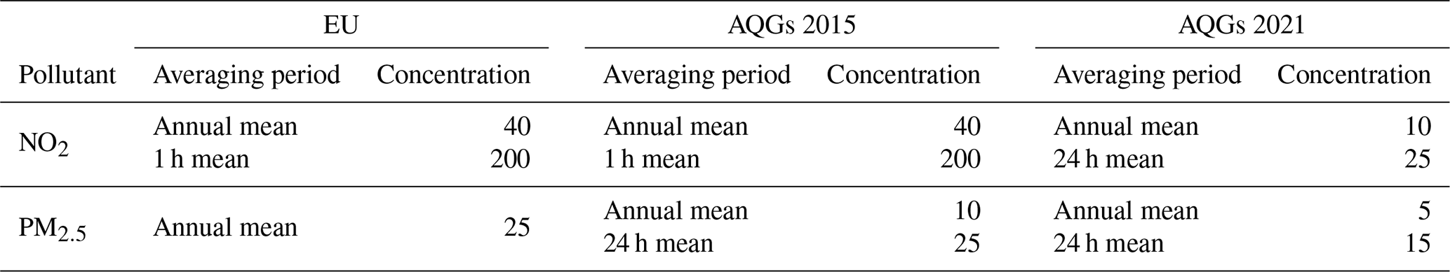
According to the World Health Organization (WHO), 7 million premature deaths every year can be attributed to poor air quality (Lelieveld et al., 2015; WHO, 2021). In response to the adverse health effects caused by air pollution, the WHO developed air quality guidelines (AQGs) for a set of key air pollutants, including nitrogen dioxide (NO2) and particulate matter with an aerodynamic diameter ≤ 2.5 µm (PM2.5) (WHO, 2021). Since the WHO's 2015 recommendation, evidence has accumulated showing many additional negative impacts of air pollution on health (Abdo et al., 2016; Sun et al., 2016; Chen et al., 2018; Ai et al., 2019; Wang et al., 2019; Wu et al., 2019; Zhang et al., 2020). After a comprehensive review of the evidence, the WHO has recently recommended a much stricter set of standards and warned that exceeding the new air quality guideline levels is associated with significant health risks. Table 1 shows the previous and revised AQGs for the pollutants of focus within this study along with the EU standards. These standards are legally binding, while the WHO values are indicative.
Table 1Air quality standards set by the European Union (Gemmer and Bo, 2013) and the WHO's global air quality guidelines (AQGs) from 2015 and 2021 (WHO, 2021). All concentrations are in µg m−3.
Traditionally, air quality monitoring is based on static air quality monitoring stations (AQMSs) with calibrated high-precision instruments. However, due to their purchase and maintenance costs, conventional AQMSs are generally sparsely located (Kumar et al., 2015; Maag et al., 2018). This monitoring strategy is suited to characterizing regional air quality but could fail to account for elevated concentrations near sources. Moreover, the temporal and spatial resolutions of such monitoring station networks are limited (Motlagh et al., 2020). For example, there are a total of 18 AQMSs in the nation of Denmark, responsible for measuring concentrations at street level, urban background, and regions – the Danish National Monitoring Programme for Water and Nature (NOVANA) (Ellermann et al., 2020).
Meanwhile, field studies have shown that pollution levels, especially in urban environments, can vary substantially within a few metres due to localized air pollution sources (Lebret et al., 2000; Kingham et al., 2000; Monn, 2001; Zou et al., 2009; Wang et al., 2018; Li et al., 2019; Wilson et al., 2019). The local component can often be an important factor contributing to people’s exposure, for example, for those who commute in a vehicle and/or work as professional drivers, street police, bicycle delivery, etc. (Frederickson et al., 2020a), or live or work in buildings near busy roads. Low-cost air pollution sensors and sensor networks have evolved rapidly during the last few decades, enabled by technological progress and the development of fast and inexpensive wireless communication systems (Snyder et al., 2013). While the technologies are still evolving, low-cost air pollution sensors are becoming available and are starting to become a valuable supplement to the sparse conventional AQMSs. Low-cost sensor (LCS)-based networks are not a substitute for networks of conventional AQMSs, since high-quality monitoring data are necessary for checking compliance with guidelines, and they are also necessary for validating less expensive mapping obtained from modelling and/or LCS-based monitoring.
Networks of low-cost air pollution sensors are becoming more common. On a device level, clearly the sensor elements cannot compete with commercial instruments regarding the three “S”s: sensitivity, stability, and selectivity (Lewis et al., 2016; Borrego et al., 2016; Castell et al., 2017; Frederickson et al., 2020b); this may be more than compensated for because LCSs enable greatly increased site density and temporal resolution, facilitating new insights into patterns and sources of air pollution. In addition, LCSs can not only supplement coarse-scale monitoring networks, but also add substantial value to mappings provided by mathematical models. Dense networks of LCSs can be used for source apportionment and to distinguish local from non-local pollution (Heimann et al., 2015) and as an aid in interpreting mathematical models that are often an integrated part of air quality monitoring (Hertel et al., 2007).
Within this study, electrochemical LCSs are used to measure gaseous pollutants, and laser-based particle counters are used to quantify particulate matter. Electrochemical sensor technology offers a number of advantages, including linear response, small size, low cost in fabrication, relatively fast response, and low power consumption (Frederickson et al., 2020b). While low-cost air pollution sensors bring new opportunities for monitoring, important issues remain regarding data quality. Studies show that sensor data can be influenced by environmental factors such as temperature and confounding gases (Spinelle et al., 2015, 2017; Mead et al., 2013; Bulot et al., 2020). Considerable efforts have been made to understand these factors, with varying success. Field work presents a complex and dynamic environment, greatly complicating the task of calibration. Experience shows that it is crucial to test each individual sensor and correct for multiple ambient factors (Popoola et al., 2016).
While a time series analysis based on summary statistics is a simple and effective tool, more sophisticated techniques are necessary to better understand the ultimate causes of these variations (Hwang and Chen, 2000). Spectral analysis using the Fourier transform can provide a deeper understanding of time series, because transformation into the frequency domain allows characterization of sources according to their periodicity and rate of change (Percival and Walden, 1998). While spectral analysis has long been used for meteorological variables, because of its ability to distinguish synoptic and seasonal signals (Van der Hoven, 1957; Lyons, 1975; Eskridge et al., 1997), studies applying the Fourier transform to air pollution data emerged much later (Rao et al., 1976; Hogrefe et al., 2006; Choi et al., 2008; Lazi et al., 2016).
There is a relation between temporal and spatial scales of air pollution (Brasseur and Jacob, 2017). Analysis of air quality data in the frequency domain contributes to the understanding of periodic behaviours and yields information about spatial and temporal scales of the hidden, underlying mechanisms (Hies et al., 2000; Sebald et al., 2000; Marr and Harley, 2002). Short-term fluctuations of the pollutant concentrations are related to local-scale phenomena, including local dispersion conditions and patterns in local emissions and chemistry. Conversely, seasonal changes and the long-range transport and emissions of pollutants contribute to the spectrum at very low frequencies (Tchepel et al., 2009). On the timescale of days, there are the motions of weather systems, for example a high-pressure system with well-developed photochemical air pollution. Pollution arriving from a distant source is characterized by a slowly rising and falling signal due to the effects of transport time and atmospheric mixing. Regional emissions are of course regional in scale, and photochemical pollution typically develops in a synoptic air mass. In contrast, local sources (e.g. traffic) more often present as a sharp spike in concentration. Even an instantaneous puff of pollution will broaden with time based on the vertical and horizontal eddy diffusion coefficients, K, which are of the order of 100 m2 s−1 (Seinfeld and Pandis, 2016).
In this paper, we show how low-cost air pollution sensors provide additional insights into the patterns and sources of air pollution when deployed as a network rather than as individual sensors. A low-cost air pollution sensor network consisting of 18 low-cost air pollution sensor nodes (called AirNode4PX) was deployed in Newcastle-under-Lyme, UK, in the area centred around the ring road (see Fig. 1). The variation in road width, the different types of road structure, and highly variable traffic patterns all impact pollutant dispersion, resulting in significant spatiotemporal variation of pollution in the area. Each AirNode measured a range of species, including nitrogen dioxide (NO2), ozone (O3), and particulate matter (PM2.5 and PM10); in this paper we focus on NO2 and PM2.5. This paper does not attempt to demonstrate that the low-cost air pollution sensors meet specific air quality monitoring standards. Rather, we argue that data obtained from such a network are able to provide useful additional information about local air pollution that extends what can be learned from conventional air quality monitoring stations. The data obtained from the low-cost air pollution sensor network are used for time series analysis in the frequency domain to obtain information on the variability of air pollution concentrations and to distinguish local sources from regional ones. The network, together with the analysis approach, has allowed pollutant emissions attributable solely to the local sources to be distinguished from other regional or long-range transport sources. The approach of frequency domain analysis will be further evaluated in subsequent studies.
In June 2020, a network of 18 air pollution sensor nodes containing low-cost electrochemical and metal oxide gas sensors and optical particle counters was deployed in Newcastle-under-Lyme in Staffordshire, UK, in the area centred around the ring road. In addition, an anemometer was installed to record wind speed and direction. The initial 14 d installation, stabilization, and testing periods of the measurement campaign are excluded from the analysis. Overall, the study covers a 14-month period from 1 August 2020 to 1 October 2021.
2.1 Nodes of low-cost air pollution sensors
The nodes include low-cost air pollution sensors, signal processing, and communications. The units, mm, are assembled by AirLabs into weatherproof enclosures with full exposure to ambient air and are set up to report measurements to a cloud hosted by Amazon Web Services. The low-cost air pollution sensor nodes are generation 4P and are referred to as AirNode, AirNode4PX, or 4PX, with X being the node number. Each AirNode includes sensors for measuring NO2 (NO2-B43F from Alphasense Ltd.) and O3 (MiCS-6814 from SGX Sensortech) as well as PM2.5 and PM10 (SDS-011 from Nova Fitness Co.) at a 1 min time resolution. In addition, each node is equipped with a control board and micro-controller unit (ESP32) for programming the sensors. The AirNodes were laboratory tested in Copenhagen, Denmark, to validate their response and obtain laboratory-based calibration coefficients, which are used to interpret the preliminary data. After laboratory calibration, the AirNodes were shipped to Newcastle-under-Lyme in Staffordshire, UK, and were mounted 2.5 to 3 m above street level on lamp posts which also provided power as shown in Fig. 1. Since the study focuses on NO2 and PM2.5, a brief description of the sensors is given below.
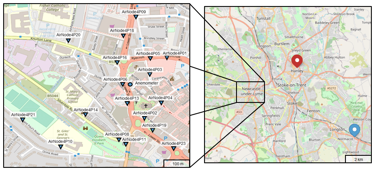
Figure 1Spatial distribution of the AirNode network (left panel) and an overview of the location of the network relative to the two closest reference stations (right panel). The urban background station at the Stoke-on-Trent centre is highlighted with a red marker, whereas the roadside monitoring station at the Stoke-on-Trent A50 roadside is highlighted with a blue marker. The last AQMS used in this study (regional background monitoring station at Ladybower) is located 54 km from the network and is for clarity not included in the map. Maps obtained from © OpenStreetMap contributors 2021. Distributed under Open Data Commons Open Database License (ODbL) v1.0 (OpenStreetMap contributors, 2021).
The SDS-011 sensor (Nova Fitness Co. Ltd, 2015) is a low-cost air pollution sensor measuring PM2.5 and PM10. Its principle of operation is based on light scattering (van de Hulst, 1981), where particle density distribution is determined using the intensity distribution patterns produced when particles scatter a laser beam (Liu et al., 2019). The sensor module includes a fan to ensure a continuous flow of air through the sensor chamber (Genikomsakis et al., 2018). An algorithm converts the particle density distribution into particle mass, and it can measure the particle density distribution between 0.3 and 10 µm (Bulot et al., 2020; Budde et al., 2018).
For NO2 measurements, the NO2-B43F sensor (Alphasense, 2019) is used. This is an amperometric electrochemical gas sensor containing four electrodes, where the principle of operation is based on electrochemistry (Frederickson et al., 2020b). When the working electrode (WE) is exposed to ambient air, the target gas can diffuse onto the surface of the electrode, where it is chemically reduced, resulting in a change in current. The counter electrode balances the current, and the reference electrode sets the operating potential of WE. The fourth electrode is an auxiliary electrode (AE) and has the same structure as WE but is not exposed to ambient air and hence is not affected by the target gas concentration, only by environmental parameters such as temperature. Therefore, the difference in voltage between the WE and AE corresponds to changes in target gas concentration at the electrochemical cell surface. A transimpedance amplifier converts the currents from the electrochemical cell into a voltage. The voltage is amplified further by a non-inverting operational amplifier, and then a 16-bit analogue-to-digital (A/D) converter (ADS1115) samples the output and produces a digital reading of the voltage level. This is used by the microprocessor to calculate the actual gas concentration (Cross et al., 2017; Stetter and Li, 2008; Mead et al., 2013). To minimize possible cross-interference from ozone, the NO2 sensors were fitted with integrated catalytic ozone filters (MnO2 filters). The performance of these filters was verified in the laboratory, and the NO2 sensors showed no significant response to ozone in the range of 0–100 ppb. Cross-interferences from other common gas pollutants were not considered important based on prior studies (Sun et al., 2017; Mead et al., 2013).
2.2 Correction methodology
The calibration of the electrochemical sensors measuring NO2 is known to vary at high (>20 ∘C) and low (<0 ∘C) temperatures and with rapid temperature change (Alphasense, 2019; Popoola et al., 2016; Li et al., 2021). Therefore, we apply a correction with coefficients determined by using a linear regression model:
where NO2 (dV) is the raw output obtained by the Alphasense NO2 cell. The NO2 (dV) readings are found from the voltage change in cell 2, which is determined by the difference between the WE and AE outputs, WE2v, and AE2v:
T is filtered temperature data obtained from the nearest reference station. Filtered temperature represents the temperature reading when ambient temperature exceeds 10 ∘C and is transformed according to
and is the rate of change in the filtered temperature. The temperature threshold of 10 ∘C was chosen because the internal temperatures of the LCS nodes often exceed the ambient temperatures, and the performance of the correction was sufficient. The linear regression coefficients, a0, a1, a2, and a3, are calculated using the method of multiple least squares, separately for each AirNode (Spinelle et al., 2017). In this formula, a3 is a measure of the sensor's sensitivity, and a0 is the offset of the sensor, whereas a1 and a2 are temperature correction coefficients.
All electrochemical sensors have a different inherent sensitivity, and hence the NO2 readings need to be scale-corrected. The scale correction is carried out by multiplying the temperature-corrected NO2 readings (NO2 (corT)), from each AirNode, by α, which is the ratio between the 0.80 and 0.20 quantiles of the NO2 readings obtained from the AirNodes (Qdiff,AirNode) and from the reference (Qdiff,Reference). The reference is the NO2 readings obtained by chemiluminescence from the reference-grade instrument at the AQMS at Stoke-on-Trent centre, 4.1 km from the network, from the same period as the measurements took place. All data from the reference station are used for the correction. The difference between the 0.80 and 0.20 quantiles is a proxy for the variation obtained in the measurements.
The offsets of the readings are determined by calculating the difference between the 0.25 quantile (Q0.25) obtained from each AirNode (Q0.25,AirNode) and from the reference (Q0.25,Reference). Hence, the offset of the temperature- and scale-corrected reading (NO2 (corT,S)) is adjusted by subtracting the calculated offset (β). The reference used in the offset correction is the same as the one used for the scale correction. The 0.25 quantile is a proxy for the measured background concentration.
where NO2 (corT,S) is the temperature- and scale-corrected NO2 reading, and NO2 (cor) is the temperature-, offset-, and scale-corrected NO2 reading.
Regarding the SDS-011 PM2.5 readings, outliers were removed by excluding all values exceeding 5 times the standard deviation. Scale and offset correction was performed for PM2.5, similarly to the one for the NO2 readings. However, there was no significant difference between the corrected and uncorrected PM2.5 readings since the PM2.5 readings were already highly correlated (mean R2=0.72) with the reference readings from the Stoke-on-Trent centre.
2.3 Comparison with regulatory air quality monitoring stations
The data obtained from the network are compared with data from the three nearest regulatory air quality monitoring stations: the roadside monitoring station at the Stoke-on-Trent A50 roadside (52.980436∘ N, 2.111898∘ W; 8.7 km from the network), the urban background monitoring station at Stoke-on-Trent centre (53.028210∘ N, 2.175133∘ W; 4.1 km from the network), and the regional background monitoring station at Ladybower (53.403370∘ N, 1.752006∘ W; 54 km from the network). We do not expect perfect agreement, but nonetheless the exercise is useful.
Ladybower is located in the Peak District National Park around 800 m to the south-west of the Ladybower reservoir. The nearest road is 20 m from the station and is only used by the nearby farmsteads. The surrounding area is mainly open moorland. The urban background monitoring station is located in Stoke-on-Trent and is in the northern part of downtown Hanley. This station is located 5 m from a road connected to a busy multi-story car parking facility (50 m from the monitoring station). The surrounding area is open grass, with a few trees and commercial properties. The A50 Potteries Way is a busy ring road which lies approximately 130 m to the north-east of the monitoring site. The roadside monitoring station is located between the main road and a parallel side road, near a pedestrian footbridge, beside the dual-carriageway A50 through Stoke. All three AQMSs are equipped with instruments for measuring NO2 by chemiluminescence, but only the Stoke-on-Trent centre measures PM2.5. Hourly air pollution data from each monitoring station were manually downloaded using the UK-Air data selector (DEFRA, 2022).
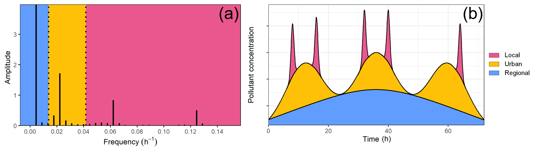
Figure 2(a) A periodogram showing short-term fluctuations at high frequencies (red), background signals at low frequencies (blue), and the fluctuations in between (yellow). (b) Schematic illustration of air pollutant contributions from regional transport (blue), the urban area (yellow), and the street (red). The relative concentration of the contributions depends on the considered pollutant and the dispersion conditions.
2.4 Spectral analysis
Spectral analysis is widely used for investigating cycles and variations of pollutants in time series to reveal the sources of pollution (Marr and Harley, 2002; Lazi et al., 2016). Within spectral analysis, the Fourier transform is a powerful tool for analysing time series including periodicities and rate of change. To use the method, it is necessary to overcome obstacles including the often unevenly spaced time points in time series due to technical and practical problems during monitoring (Sun and Wang, 1996, 1997). The unequally spaced or missing data can be circumvented by applying the fast Fourier transform after filling the gaps and missing values with the mean. In addition, the linear trend in the time series is removed by subtracting the average concentration obtained by each LCS. The periodogram for a finite time series is calculated as the square of the magnitude of X:
where k=0, 1, …, N−1, and N is the number of observations, xt is the time series, and . The periodogram indicates the strength of the signal as a function of frequency, while its spectrum over the frequency range corresponds to the variance of the time series data. Parseval's theorem (Narayanan and Prabhu, 2003) states that the energy, or in this case intensity, is conserved during Fourier transformation. Thus, the contribution of the different pollution sources can be quantified by integrating the peaks in the periodograms (Marr and Harley, 2002).

Figure 3Daily patterns of NO2 measured by the reference instrument (blue), corrected NO2 concentrations (red) measured by one representative node (AirNode4P01), and uncorrected NO2 concentrations (yellow) measured by AirNode4P01 during weekdays (a) and weekends (b). Note the different-scale y axis. The shading shows the 95 % confidence intervals of the mean. Please note that NO2_raw represents the Alphasense NO2 cell output (dV) multiplied by the scale coefficient obtained from the laboratory calibration. The plots are produced by timeVariation{openair} (Carslaw and Ropkins, 2012).
There is a relationship between temporal and spatial scales of the different air pollutants. Rapid, short-term fluctuations of the pollutant concentrations happen as a result of local phenomena, e.g. local-scale dispersion, local emissions, and short-term atmospheric chemistry. Rapid changes contribute to the periodogram at high frequencies, which in this work are defined as above 0.0417 h−1, i.e. events with a frequencies higher/shorter than 1 d. This is referred to as the “local” contribution to the pollutant concentration. The local cutoff is chosen based on the European Environment Agency's definition of a local timescale (EEA, 2008). The seasonal changes in the emissions and long-range transport of the pollution contribute to the periodogram at low frequencies (<0.0139 h−1), i.e. events with a frequency lower/longer than 3 d. This is then referred to as the “regional” contribution to the pollutant concentration. In this model, intermediate frequencies are due to the “urban” contribution to the pollutant concentration. The cutoff frequency for the regional contribution is based on the intercontinental transport, which occurs on timescales of the order of 3 d to 1 month (Stohl et al., 2002). As noted in the introduction, the mixing of pollution with time provides an upper limit on frequency for distant sources; only local sources can give a high-frequency signal. The above-mentioned definitions are illustrated in Fig. 2. One of the properties of diffusion is that a pulse of pollution will propagate in a Gaussian concentration profile depending on the diffusion constant and time. Under the Fourier transform, a Gaussian is mapped onto another Gaussian with a different width. The transform of a wide function is narrow and vice versa. By integrating periodograms in the three different frequency bins by the equations below, the relative contribution of local, urban, and regional pollution of the LCS data can be quantified.
where νstart and νend are the start and end frequencies in the chosen frequency bins, which is elaborated below.
g is non-negative and square-integrable with respect to the Lebesgue measure on νk. After the relative contributions are calculated for each LCS node, the average concentration together with the standard deviation can be calculated across the AirNode network to illustrate how much local pollution the network is seeing on average and how much variation is seen across all AirNodes.
In the following section, we present the results of our study and of the data analysis.
3.1 Sensor data quality
The first requirement is to establish the fidelity of the monitoring network.
3.1.1 Missing data
The data completeness of the AirNodes varies between sites. In the monitoring network, apart from four AirNodes (4P04, 4P06, 4P08, and 4P20), all AirNodes have more than 80 % data completeness during the sampling period. The four AirNodes with data completeness below 80 % were excluded from the analysis. Across the network of AirNodes, the mean data completeness is 95 %, which is sufficient for investigating the local variation of air pollution. The main reasons for data gaps are the irregularities in the line power and lapses in the wireless internet connection. In addition, spiders had in a few cases entered through the small holes at the base of the AirNodes and nested in the housing, leading to sensor failure.
3.1.2 Correction of NO2 readings
It is necessary to account for temperature bias while deploying electrochemical NO2 sensors (Alphasense, 2014). For our study, this correction was crucial in order to get meaningful readings from the electrochemical sensors since the raw readings showed unphysical behaviour. The typical NO2 patterns during weekdays (Monday to Friday) and weekends (Saturday and Sunday) measured by AirNode4P01 as an example are shown before and after the correction in Fig. 3. All AirNodes have the same tendencies, so Fig. 3 is characteristic of all AirNodes. For clarity, the NO2_raw represents the Alphasense NO2 cell output (dV) multiplied by the scale coefficient obtained from the laboratory calibration. The NO2 patterns of the corrected NO2 readings compared to the readings from the reference indicate that the correction procedure can overcome most of the disparity between the readings during higher temperatures. Modeled temperature data from DEFRA (DEFRA, 2022) are used to correct for the temperature bias. The correction coefficients for the AirNodes were calculated for each individual AirNode, and the mean and standard deviation of the correction coefficients are a0=20.83 (13.29), (0.17), a2=1.37 (0.58), and a3=892.38 (521.02). All four terms in the linear regression model have a p value of below 0.05 for all AirNodes. The relatively high standard deviations are linked to the known intra-sensor variability and show that each sensor requires individual calibration and/or correction. The correction coefficient, a0, or offset of the sensor is higher than the average concentration, and it has a relatively high standard deviation. This is a property of the Alphasense cell and can vary significantly from cell to cell, which underscores the importance of calibrating and correcting the raw data from low-cost sensors in order to obtain accurate concentrations.
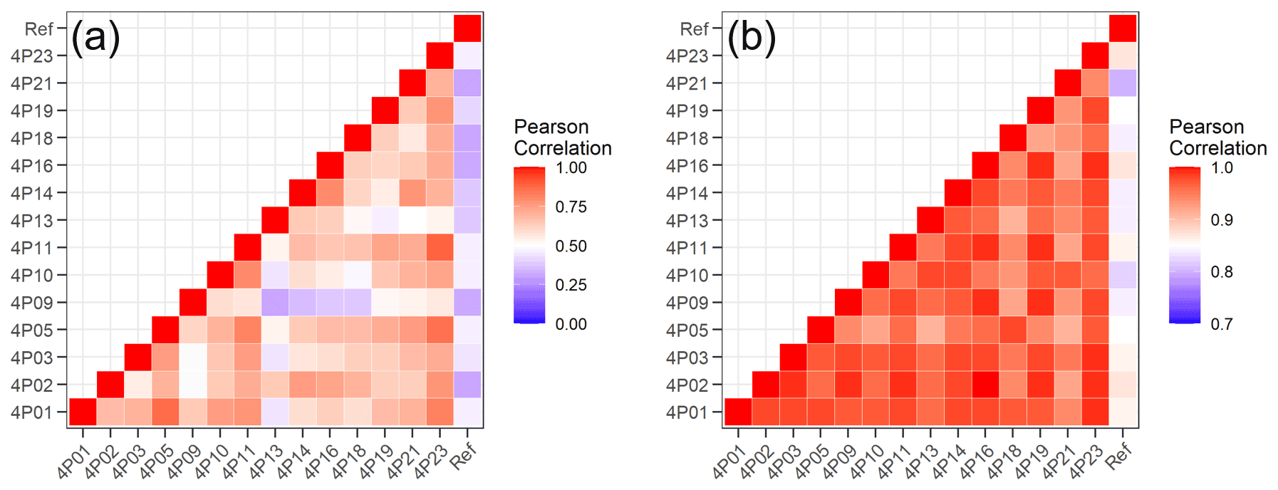
Figure 4Correlation heatmap of the Pearson correlation coefficient for NO2 (a) and PM2.5 (b). Note the different scales.
It is known that in cities the temperature can vary strongly over small distances (Cao et al., 2021), and therefore it would have been more accurate to measure the internal temperature of the AirNodes and use that information for the correction. However, the correction methodology even with the modeled temperature data yields corrected readings that follow expected trends, giving confidence in sensor accuracy. However, as seen in Fig. 3, there is still a relatively large discrepancy between the reference and corrected AirNode readings on weekdays between 8 and 12 h, which can be attributed to the large distance between the reference instrument and the AirNodes (4.1 km) and the fact that the concentration of NO2 can have different profiles at different locations, depending on the traffic modes and sources. Sensor performance is validated below.
3.1.3 Inter-sensor variability
Inter-sensor variability has been used as a metric of sensor reliability in recent studies (Liu et al., 2020). Figure 4 displays the correlation heatmap of the Pearson correlation coefficient for NO2 and PM2.5, in which the respective reference measurements from the Stoke-on-Trent centre are included. The Pearson correlation coefficients for PM2.5 among the AirNodes ranged from 0.87 to 0.99 with a mean of 0.95. In contrast, the Pearson correlation coefficients for NO2 ranged from 0.30 to 0.88 with a mean of 0.64. For PM2.5, the lowest Pearson correlation coefficients were above our quality criterion of 0.85. We did not choose a similar criterion for NO2 since we expect there is much higher variation between the sensors due to localized sources. The AirNode network readings rose and fell simultaneously as ambient concentrations and conditions changed, confirming that the sensors are operating as expected and giving confidence in sensor measurement reliability. The AirNode readings generally followed the same trends as seen at the reference instruments at Stoke-on-Trent centre. The mean Pearson correlation coefficient for NO2 was 0.40 with a range of 0.3 to 0.47, whereas the mean Pearson correlation coefficient for PM2.5 was 0.85 with a range of 0.80 to 0.87. Again, the larger discrepancy between the reference and corrected NO2 readings can be attributed to the more spatially variable nature of NO2.
3.2 Descriptive statistics
Air quality data for NO2 and PM2.5 measured at the different sites during 2020 and 2021 were analysed. For this section, only 1 year of data (1 August 2020 to 1 August 2021) is used to compare with official guidelines. Descriptive statistics of the air quality measurements are presented in Table 2. The mean concentrations are compared with the WHO's recently updated European AQGs and the legally binding EU standards; see Table 1. It should be noted that the legally binding values for annual means are defined for 1 January to 31 December. The mean annual NO2 and PM2.5 concentrations across the network exceed the updated WHO guidelines by 7 and 3 µg m−3 for NO2 and PM2.5, respectively. All sites have days where the daily average NO2 and PM2.5 concentrations exceed the WHO daily average AQG limits during the period. However, none of the sites are above the legally binding EU standards.
Table 2Statistics for air quality data measured from 1 August 2020 to 1 August 2021. For comparison, the descriptive statistics from the three regulatory air quality monitoring stations (regional: Ladybower, urban background: Stoke-on-Trent centre, roadside: Stoke-on-Trent A50 roadside) are shown for the corresponding period. Neither Ladybower nor the Stoke-on-Trent A50 roadside has instruments for monitoring PM2.5. Abbreviations: SD: standard deviation, max: maximum value. We are aware that the measurement uncertainty is significantly higher for low-cost air pollution sensors than for reference air quality monitoring measurements. However, EU air quality guidelines approve low-cost sensor data as indicative but not quantitative data – in line with calculations with air quality models.
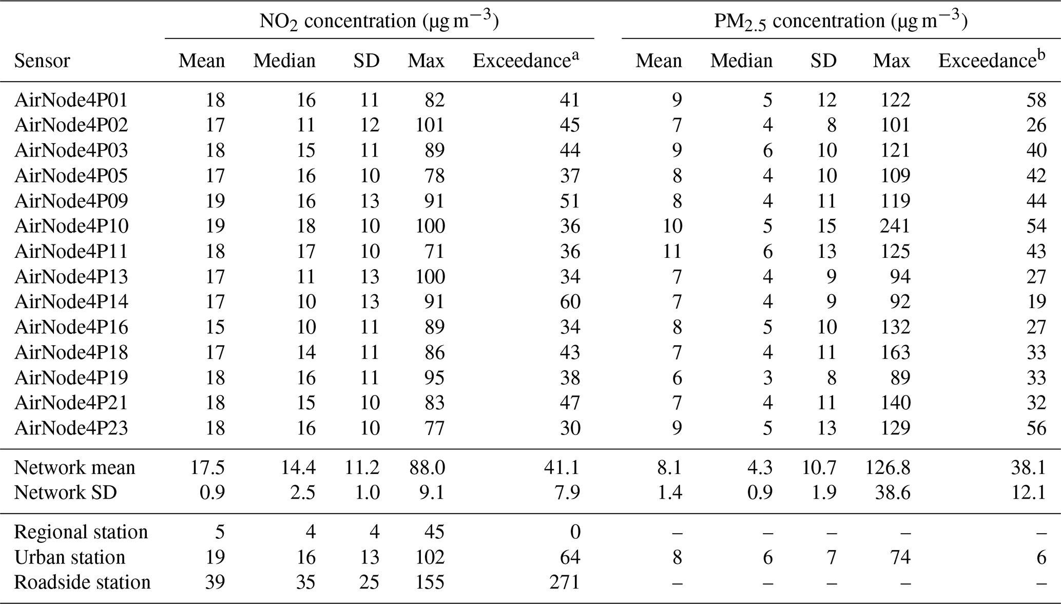
a Number of days with an average NO2 concentration above the WHO's guideline of 25 µg m−3. b Number of days with an average PM2.5 concentration above the WHO's guideline of 15 µg m−3.
The values obtained from the network can be analysed in relation to the values reported by AQMSs, as long as the significant distance between the measurement locations is kept in mind. The values from the network are compared with the three AQMSs: the monitoring station at the Stoke-on-Trent A50 roadside, the urban background monitoring station at the Stoke-on-Trent centre, and the regional background monitoring station at Ladybower. Only the urban background station at the Stoke-on-Trent centre is reported in PM2.5. Concentrations of NO2 and PM2.5 (when available) are averaged within the same period as the AirNodes in the network (i.e. 1 August 2020 to 1 August 2021), and the descriptive statistics are shown in Table 2. The mean concentrations obtained from the network show similar values for NO2 and PM2.5 to those seen at the urban background station. On average, while the network sees lower NO2 values than the roadside monitoring station (21.4 µg m−3), there is an NO2 excess relative to the regional background exposure (12.5 µg m−3). In an environment such as a city with an elevated urban background concentration, exposure to air pollution in micro-environments can cause exceedance of recommended threshold values for many individuals, in addition to the dangers of transient and continued exposure.
3.3 Temporal trends
Figure 3 shows the temporal variation in NO2. On weekdays, the NO2 concentration increases in two time periods during the day, with peaks at 07:00 and 18:00 LT. On weekends, the NO2 concentration rises steadily throughout the day. There is a notable decrease in concentration during the weekend compared to the weekdays at all sites. For both weekends and weekdays, the NO2 concentration is lowest at night. The two time periods with increased NO2 concentration during the weekdays are typically periods of increased traffic during morning and afternoon rush hours when people commute to and from work (Vignati et al., 1996; Berkowicz et al., 1996). Thus, traffic likely drives this observed variation, in line with the declining NO2 concentration during the night and over the weekend.

Figure 5Monthly variation of NO2 measured by one representative node (AirNode4P10) (red) and the corresponding reference instrument at Stoke-on-Trent centre (blue). The plot is produced by timeVariation{openair} (Carslaw and Ropkins, 2012).
In terms of monthly trends, Fig. 5 displays the monthly average of the NO2 concentration measured by one of the AirNodes together with the monthly readings from the nearest urban background AQMS (Stoke-on-Trent centre). All AirNodes have the same tendencies, so Fig. 5 is characteristic of all AirNodes. The readings from the AirNode and the AQMS follow the same trends, with the highest NO2 concentrations in the spring and the winter.
3.4 Spatial trends
Wind speed and direction have been shown to provide essential information that can help identify source locations (Carslaw et al., 2006; Westmoreland et al., 2007). The description of variation with wind direction and wind speed on a specific street (the so-called street canyon effect) is given in Berkowicz et al. (1996). Bivariate polar plots are a powerful tool for source characterization including mean pollutant concentrations for specific wind speed and direction bins (Uria-Tellaetxe and Carslaw, 2012; Grange et al., 2016; Carslaw and Ropkins, 2012; Carslaw and Beevers, 2013). In these plots wind direction is displayed from 0 to 360∘ clockwise on the angular axis, and wind speed is shown on the radial scale.
The wind speed and direction data used in this study are shown as a wind rose in Fig. 6. The wind rose shows that the prevailing winds come from the south and north-west during the measurement period. To assess spatially resolved source patterns, bivariate polar plots of the NO2 and PM2.5 are investigated. The bivariate polar plots for each pollutant for all sites are shown in Fig. 7. Reddish colours represent higher values compared to the blueish ones.
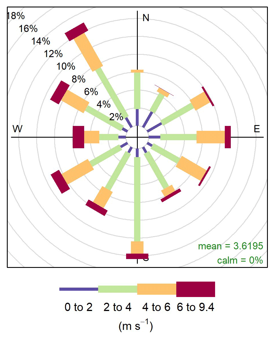
Figure 6Wind rose showing the frequency of counts by wind direction (%). The plot is produced by windRose{openair} (Carslaw and Ropkins, 2012).
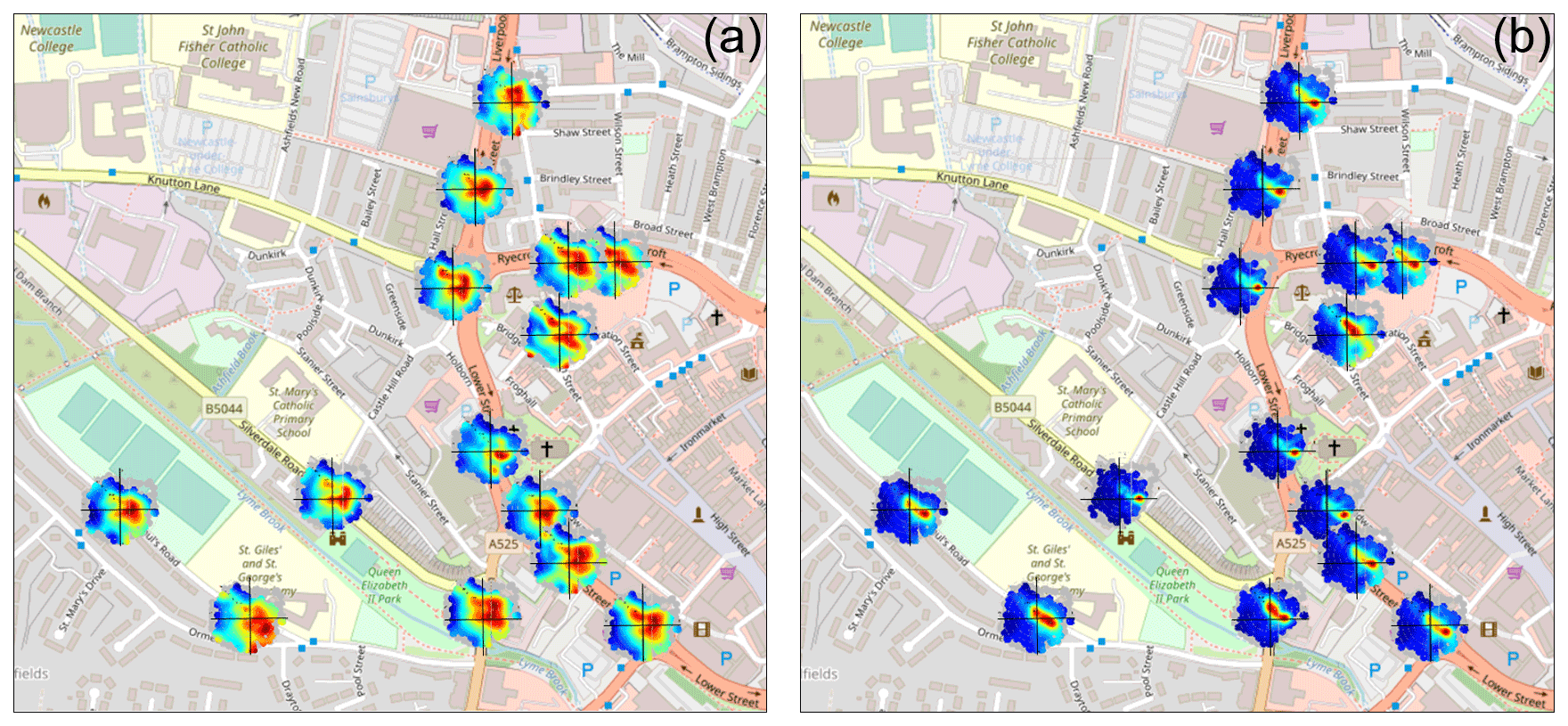
Figure 7Bivariate polar plots of NO2 (a) and PM2.5 (b) show the spatial variability in the study area for the entire study period. The figures are produced by polarMap{openairmaps} (openairmaps is a package that supports openair (Carslaw and Ropkins, 2012) for plotting on various maps), where the maps are obtained from © OpenStreetMap contributors 2021. Distributed under Open Data Commons Open Database License (ODbL) v1.0 (OpenStreetMap contributors, 2021).
The bivariate polar plots show patterns that depend on deployment location. AirNode4P23, AirNode4P19, and AirNode4P02 are located in the southern part of the ring road, and they display similar patterns in their bivariate polar plots. Their surroundings are almost identical, and the traffic influence on their readings is similar. The nodes located in the northern part of the ring road have different patterns relative to the ones in the southern area. They experience the highest values at lower wind speeds. When peak concentrations occur at low wind speeds, it suggests local sources. For example, in a street canyon, there is both a direct and recycled contribution to the concentration, where the relative size of these two contributions depends on whether the measuring site at a given time is on the leeward or windward side of the street. AirNode4P10 is located in front of a school, and at lower wind speeds or with westerly wind, elevated levels of NO2 were observed. In general, the highest concentrations are observed at low wind speeds, where no whirlwind is formed inside the street, independent of wind directions, or when the measuring site is on the leeward side of the street (in relation to the whirlwind). In the latter case, pollution from the traffic in the specific section of the street will be led directly to the measuring site, at the same time as there is a contribution due to trapping of pollution within the limited volume of the whirlwind.
Higher NO2 values are correlated with wind speed and the orientation of the road. The traffic comes from the ring road area and continues through St Paul's Road. Near the school, traffic stops frequently and accelerates and idles while children are being dropped off and picked up. The lowest values of NO2 are seen at higher wind speeds with north-westerly winds. The bivariate polar plots for AirNode4P01 and AirNode4P05 show similar patterns, with the highest concentrations found for easterly and south-westerly winds, whereas the lowest concentrations were seen with westerly and south-westerly winds. Higher-speed south-westerly winds contributed to the peak concentrations at these locations. A wide-open parking area is located next to the ring road in that direction, which could explain the elevated concentrations.
The wind speed dependence of concentrations in a street canyon can be complex, as there are opposing effects: higher wind speeds lead to more O3 but also more dilution of NOx (NO + NO2). High wind speeds will therefore lead to lower NO2, while at low wind speeds, NO2 formation is limited by O3, which goes towards zero in the street (Palmgren et al., 1996). Bivariate polar plots are good at revealing these interrelationships. The wind speed dependence can help distinguish sources from one another. When several measurement sites are available, polar plots can triangulate different sources (Carslaw et al., 2006). As expected, NO2 is dominated by local emissions, and peak values mainly occur for low wind speeds, where elevated concentrations were observed due to accumulation and lack of dispersion. The most obvious features of NO2 bivariate polar plots are that the elevated levels are attributable to the orientation of the road or the place with the highest traffic density.
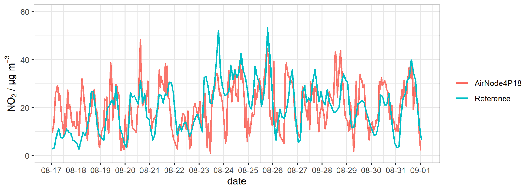
Figure 8Time series of NO2 measured by one representative AirNode (AirNode4P18) with a time resolution of 30 min and the corresponding reference instrument at Stoke-on-Trent centre with a time resolution of 1 h. For clarity, only 2 weeks of data are shown.
Relative to the bivariate polar plots of NO2, the bivariate polar plots of PM2.5 do not show as much variation across the network. Generally, the highest concentrations of PM2.5 are seen for south-easterly winds and higher wind speeds. This is confirmed by the frequency spectrum showing slow changes consistent with large air masses. This indicates that particles originate from long-range transport. The bivariate polar plots for PM2.5 also suggest that the locally sourced particulate matter is present, shown by the elevated concentrations at low wind speeds, where the atmospheric conditions are more stable.
In general, sites across the sensor network show a variation in their bivariate polar plots (however, more for NO2 than for PM2.5) due to the different pollution sources. Thus, there are additional benefits of multi-sensor node measurements for characterizing sources in detail, especially when combining them with meteorological information.
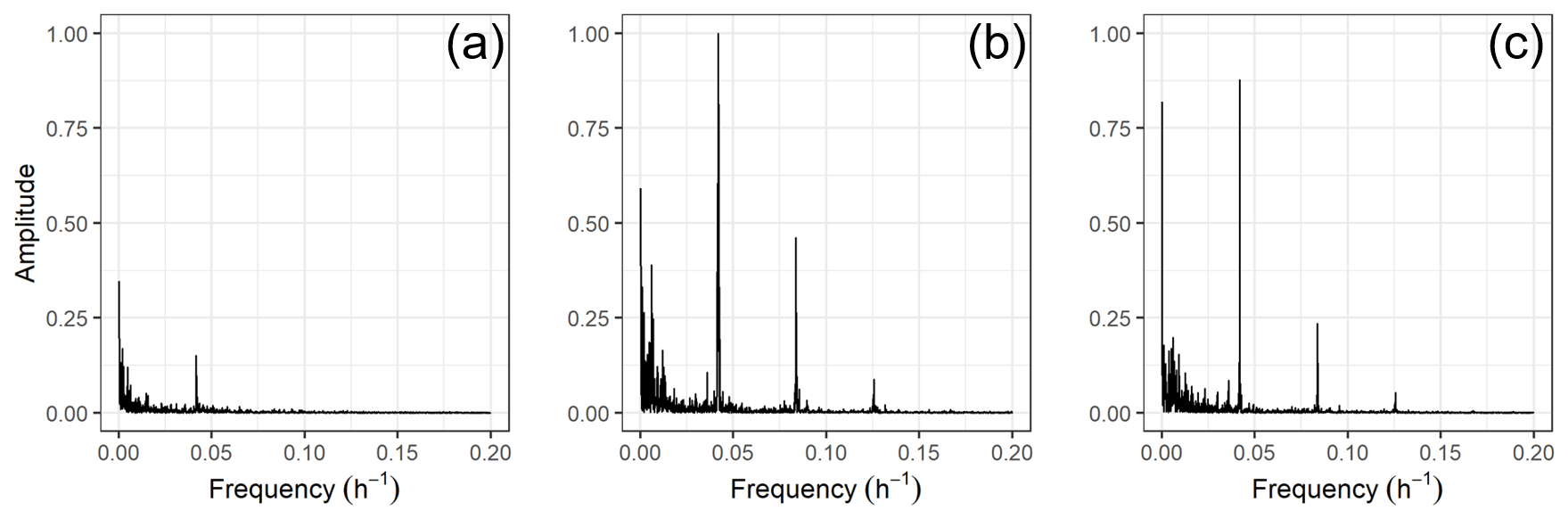
Figure 9Periodograms for NO2 at regional background AQMS, Ladybower (a), street AQMS, Stoke-on-Trent A50 roadside (b), and urban background AQMS, Stoke-on-Trent centre (c). All periodograms are normalized against the highest peak.
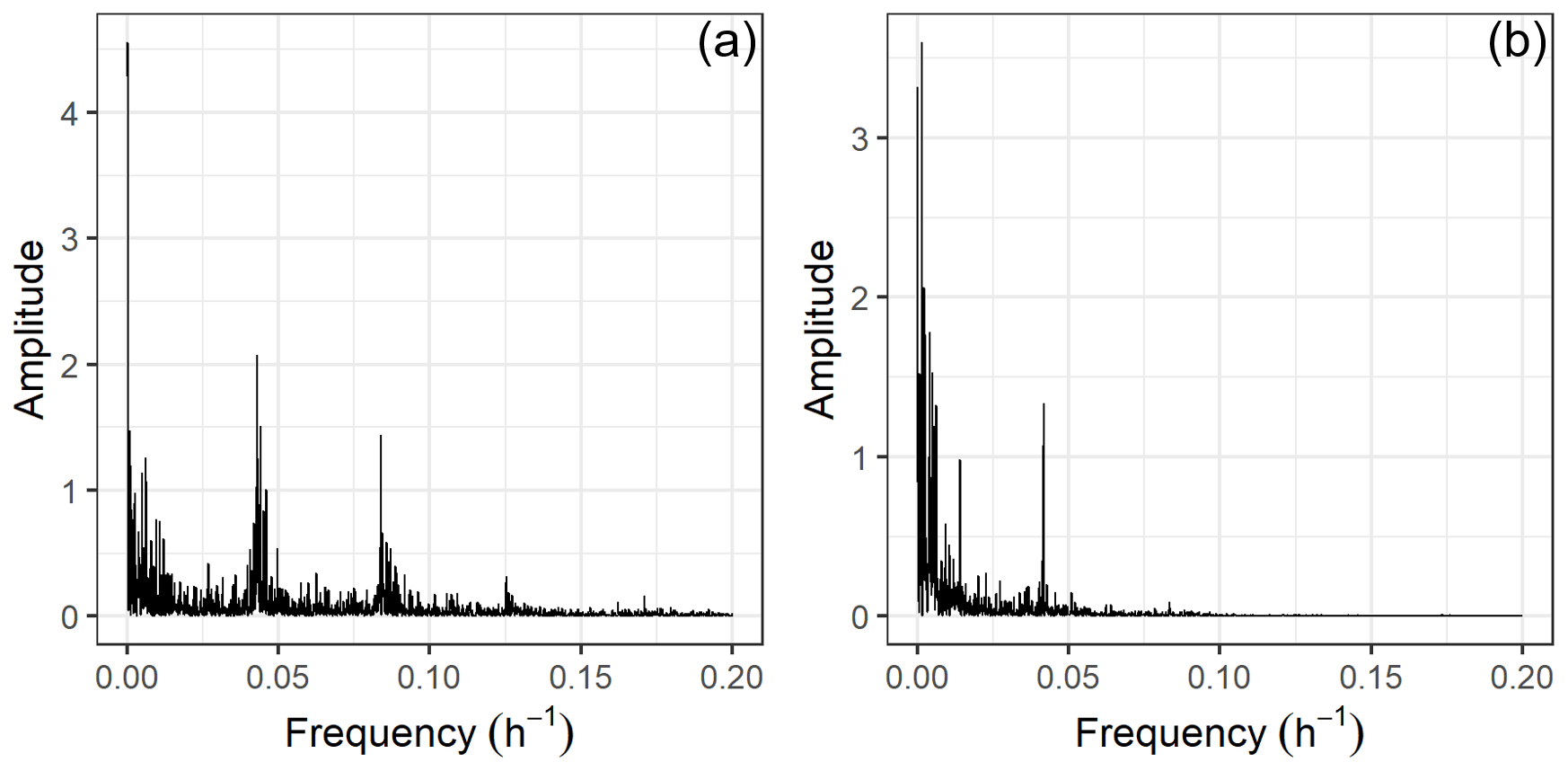
Figure 8 shows data from the urban background AQMS at the Stoke-on-Trent centre at a time resolution of 1 h (DEFRA, 2022). Data from one of the AirNodes with a time resolution of 30 min are shown for comparison. The raw readings from the AirNodes have a time resolution of 1 min; however, the temperature correction aggregates the data into 30 min bins. Still, with a time resolution of 30 min, we see more local variability in the data compared to the readings from the reference station. The data have a measurement density in both time and space, which cannot be achieved using current conventional measurement methods. As seen in Fig. 8, the readings from the AirNode and the AQMS follow the same trend, but the correlation of determination is only 0.28. This is expected, since the AQMS is located around 4 km from the AirNode network. However, increasing the time resolution will increase the correlation of determination; i.e. a time resolution of 3 h results in a correlation of determination of 0.38, and a time resolution of 1 d yields 0.63.
3.5 Spectral analysis
Spectral analysis is performed on the air pollution data to investigate its hidden periodicities and to quantify their magnitude. The contributions of local and regional sources to the pollution concentrations are determined based on the determined amplitudes and frequencies. The local sources are shown in the high-frequency periodogram, and the regional or long-range sources are revealed in the low-frequency periodogram. Note however that local sources may be present in both the low- and high-frequency regions. For example, in an urban street, the traffic patterns follow stable patterns with daily and weekly periodicities. Holiday periods follow their own pattern, and for wood smoke, emissions follow variations in outdoor temperature. By comparing the spectra for the different pollutants measured by the same AirNode, information on the sources can be revealed. If the emission sources for the different pollutants are the same, similar cyclic patterns can be expected. The differences in the pollution spectra can indicate a contribution from the different pollutant sources or the presence of chemical transformation since all other conditions are identical.
Spectral analysis is performed on NO2 data from three different types of AQMSs to illustrate how periodograms vary depending on location. These AQMSs are (1) regional background (Ladybower), (2) urban background (Stoke-on-Trent centre), and (3) street (Stoke-on-Trent A50 roadside). The three periodograms are shown in Fig. 9. While all three periodograms have significant peaks in the low-frequency region, only the urban background and street AQMSs have significant peaks in the high-frequency region. We conclude that these high-frequency peaks are due to the proximity and strength of local NO2 sources.
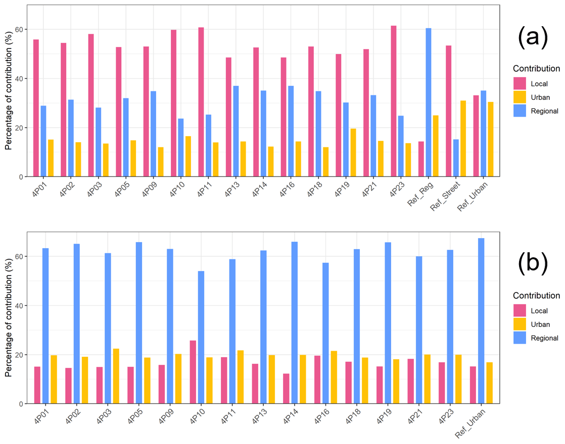
Figure 11Histogram of percentages of contribution (%) of local (red), urban (yellow), and regional sources (blue) for NO2 (a) and PM2.5 (b) measured by all AirNodes in the network as well as for the three AQMS. Ref_Reg is the regional background AQMS, Ladybower, Ref_Street is the street AQMS, Stoke-on-Trent A50 roadside, and Ref_Urban is the urban background AQMS, Stoke-on-Trent centre.
Figure 10 displays the periodograms for NO2 and PM2.5 measured by AirNode4P01. The periodogram of NO2 features three distinct peaks at 0.125, 0.084, and 0.042 h−1 corresponding to periods of 8, 12, and 24 h, respectively. In addition, one peak is identifiable in the high-frequency region at 0.17 h−1 (6 h). In the low-frequency region, there are multiple peaks close to each other; however, the peaks corresponding to 5 d (0.0083 h−1), 1 week (0.0061 h−1), and 1 month (0.00135 h−1) can still be identified. All these cycles can be related to local sources of pollution, e.g. traffic or meteorological changes. Peaks located in the low-frequency region can originate from changes over either a synoptic or larger scale. The highest intensity occurs in the high-frequency region since most of the NO2 originates from local sources. The daily changes in NO2 concentrations can be associated with the daily changes in traffic from nearby roads and the diurnal variation caused by sunlight. Weekly periodicity may also originate from changes in traffic.
The periodogram for PM2.5 (see Fig. 10) features one distinct peak in the high-frequency region at 0.042 h−1 (24 h) and a prominent peak at 0.084 h−1 (12 h). Besides these two peaks, most peaks are seen in the low-frequency region of the periodogram, which is expected since PM2.5 is dominated by long-range transport and non-local sources. However, the contribution by PM from a nearby road can originate from traffic, since vehicles, in general, can re-suspend particles from the road into the air, and abrasion from brakes and tires also produces PM (Grigoratos and Giorgio, 2015).
Periodograms for the rest of the AirNodes in the network show results similar to the ones shown in Fig. 10, with small changes in position and amplitude at specific locations. Conclusions regarding trends in pollution sources can be drawn by examining the relative contributions from local, urban, and regional sources. Figure 11 shows the calculated percentages of local, urban, and regional contributions for the AirNodes as well as for the three different types of AQMSs. The results for the network indicate that local emissions are the most important source of NO2 with an average of 54.3±4.3 %, whereas PM2.5 is mainly due to regional sources (62.1±3.5 %). For NO2, urban sources contribute 14.3±1.9 % and regional sources 31.2±4.5 %. For PM2.5, urban sources contribute 20.0±1.2 % and local sources 17.9±3.2 %.
As expected, the regional background AQMS shows the highest relative contribution from regionally sourced NO2, and the street AQMS has the highest level of locally sourced NO2. The AirNodes in the network show a distribution of contributions.
The results obtained for both NO2 and PM2.5 reveal contributions of short-term (12 and 24 h) and long-term fluctuations. The contributions at low frequencies are significantly different between the two pollutants, indicating that temporal variations are influenced by different processes. The methodology is a powerful tool for analysing the causes of air pollution.
Air pollution can be hyper-local, and low-cost air pollution sensors are capable of accurately describing variation close to pollution sources. This study assessed more than 1 year of NO2 and PM2.5 data with high spatiotemporal resolution (1 min) obtained using a network of 18 low-cost air pollution sensor nodes. Initially, there were significant calibration issues associated with temperature bias in the NO2 readings, but a simple and effective temperature, scale, and offset correction was able to overcome this problem. Therefore, this study, like many others, clearly indicates that while low-cost air pollution sensors can be useful, calibration and correction are far from trivial and require supporting data from reference stations. The corrected NO2 concentrations have a strong connection with the reference station used, so results reflect both the low-cost air pollution sensor data and reference station data.
In its recent update and revision of the air quality guidelines for Europe, the WHO has proposed annual NO2 and PM2.5 exposure guideline thresholds of 10 and 5 µg m−3, respectively. The annual mean NO2 and PM2.5 concentrations across the network exceed the updated WHO guidelines by 7 µg m−3 for NO2 and 3 µg m−3 for PM2.5. However, none of the sites had values exceeding the legally binding UK/EU standards. An excess concentration of 12.5 µg m−3 of NO2 in the network was seen relative to background levels measured by the regional monitoring station at Ladybower reservoir. This highlights the risk of pollution exposure for individuals due to local sources and supports the use of local monitoring to characterize the risk.
Spectral analysis is found to be a good method for studying the variation within the time series. This approach enabled the detection of different underlying periodicities in time series data and allowed the pollution signal to be apportioned to different categories of pollution sources, whether local, urban, or regional. The results highlighted the advantages of having a densely deployed sensor network over the sparse conventional air quality monitoring stations. The highly increased spatiotemporal resolution of low-cost sensors combined with their dense placement near pollution sources makes it possible to provide additional information on the patterns and sources of air pollution, which in turn provides a better description of the highly variable and complex nature of pollution.
All raw data are available upon request.
LBF and MSJ conceptualised the project, together with its methodology. RS and JAS were responsible for software and helped LBF with data curation. LBF carried out the formal analysis, investigation, and visualisation and took the lead in writing the manuscript with supervision from JAS, OH and MSJ. MSJ and OH were responsible for funding acquisition. All the authors provided critical feedback and helped shape the research, analysis and manuscript.
RS, JAS, and MSJ are employees of AirLabs, and LBF is partly funded by AirLabs. AirLabs made the sensor nodes used in this study.
Publisher's note: Copernicus Publications remains neutral with regard to jurisdictional claims in published maps and institutional affiliations.
The authors thank Bartosz Gaik and Archie Waller for their dedicated and professional assistance with logistical and technical issues. The authors thank © OpenStreetMap contributors 2021 for map data, available from https://www.openstreetmap.org (last access: 1 August 2022), and David Carslaw for providing the online available openair package in R. Louise Bøge Frederickson is supported by BERTHA – the Danish Big Data Centre for Environment and Health funded by the Novo Nordisk Foundation Challenge Programme (grant NNF17OC0027864).
This research has been supported by BERTHA – the Danish Big Data Centre for Environment and Health funded by the Novo Nordisk Foundation Challenge Programme (grant no. NNF17OC0027864).
This paper was edited by Tanja Schuck and reviewed by two anonymous referees.
Abdo, N., Khader, Y. S., Abdelrahman, M., Graboski-Bauer, A., Malkawi, M., Al-Sharif, M., and Elbetieha, A. M.: Respiratory health outcomes and air pollution in the Eastern Mediterranean Region: a systematic review, Environ. Health Rev., 31, 259–280, https://doi.org/10.1515/reveh-2015-0076, 2016. a
Ai, S., Wang, C., Qian, Z.M., Cui, Y., Liu, Y., Acharya, B. K., Sun, X., Hinyard, L., Jansson, D. R., Qin, L., and Lin, H.: Hourly associations between ambient air pollution and emergency ambulance calls in one central Chinese city: Implications for hourly air quality standards, Sci. Total Environ., 696, 133956, https://doi.org/10.1016/j.scitotenv.2019.133956, 2019. a
Alphasense: Alphasense application note 803: Correcting for background currents in four electrode toxic gas sensors, Technical report AAN 803-01, Alphasense Ltd, https://zueriluft.ch/makezurich/AAN803.pdf (last access: 4 September 2022), 2014. a
Alphasense: Technical specification NO2 Sensor, NO2-B43F Nitrogen Dioxide Sensor 4-electrode, Version V1, Data sheet, https://www.alphasense.com/wp-content/uploads/2019/09/NO2-B43F.pdf (last access: 4 September 2022), 2019. a, b
Berkowicz, R., Palmgren, F., Hertel, O., and Vignati, E.: Using measurements of air pollution in streets for evaluation of urban air quality – meteorological analysis and model calculations, Sci. Total Environ., 189/190, 259–265, https://doi.org/10.1016/0048-9697(96)05217-5, 1996. a, b
Borrego, C., Costa, A. M., Ginja, J., Amorim, M., Coutinho, M., Karatzas, K., Sioumis, T., Katsifarakis, N., Konstantinidis, K., De Vito, S., Esposito, E., Smith, A. N., Gérard, P., Francis, L. A., Castell, N., Schneider, P., Viana, M., Minguillón, M. C., Reimringer, W., Otjes, R. P., von Sicard, O., Pohle, R., Elen, B., Suriano, D., Pfister, V., Prato, M., Dipinto, S., and Penza, M.: Assessment of air quality microsensors versus reference methods: The EuNetAir joint exercise, Atmos. Environ., 147, 246–263, https://doi.org/10.1016/j.atmosenv.2016.09.050, 2016. a
Brasseur, G. and Jacob, D.: Modeling of Atmospheric Chemistry, Cambridge University Press, Cambridge, https://doi.org/10.1017/9781316544754, 2017. a
Budde, M., Schwarz, A. D., Müller, T., Laquai, B., Streibl, N., Schindler, G., Köpke, M., Riedel, T., Dittler, A., and Beigl, M.: Potential and limitations of the low-cost SDS-011 particle sensor for monitoring urban air quality, ProScience, 5, 6–12, https://doi.org/10.14644/dust.2018.002, 2018. a
Bulot, F. M. J., Russell, H. S., Rezaei, M., Johnson, M. S., Ossont, S. J. J., Morris, A. K. R., Basford, P. J., Easton, N. H. C., Foster, G. L., Loxham, M., and Cox, S. J.: Laboratory comparison of low-cost particulate matter sensors to measure transient events of pollution, Sensors, 20, 2219, https://doi.org/10.3390/s20082219, 2020. a, b
Cao, J., Zhou, W., Zheng, Z., Ren, T., and Wang, W.: Within-city spatial and temporal heterogeneity of air temperature and its relationship with land surface temperature, Landsc. Urban Plan., 206, 103979, https://doi.org/10.1016/j.landurbplan.2020.103979, 2021. a
Carslaw, D. C. and Beevers, S. D.: Characterising and understanding emission sources using bivariate polar plots and k-means clustering, Environ. Model. Softw., 40, 325–329, https://doi.org/10.1016/j.envsoft.2012.09.005, 2013. a
Carslaw, D. C. and Ropkins, K.: openair – An R package for air quality data analysis, Environ. Model. Softw., 27–28, 52–61, https://doi.org/10.1016/j.envsoft.2011.09.008, 2012. a, b, c, d, e
Carslaw, D. C., Beevers, S. D., Ropkins, K., and Bell, M. C. Detecting and quantifying the contribution made by aircraft emissions to ambient concentrations of nitrogen oxides in the vicinity of a large international airport, Atmos. Environ., 40, 28, 5424–5434, https://doi.org/10.1016/j.atmosenv.2006.04.062, 2006. a, b
Castell, N., Dauge, F. R., Schneider, P., Vogt, M., Lerner, U., Fishbain, B., Broday, D., and Bartonova, A.: Can commercial low-cost sensor platforms contribute to air quality monitoring and exposure estimates?, Environ. Int., 99, 293–302, https://doi.org/10.1016/j.envint.2016.12.007, 2017. a
Chen, G., Guo, Y., Abramson, M. J., Williams, G., and Li, S.: Exposure to low concentrations of air pollutants and adverse birth outcomes in Brisbane, Australia, 2003–2013, Sci. Total Environ., 622, 721–726, https://doi.org/10.1016/j.scitotenv.2017.12.050, 2018. a
Choi, Y.-S., Ho, C.-H., Chenb, D., Noha, Y.-H., and Song, C.-K.: Spectral analysis of weekly variation in PM10 mass concentration and meteorological conditions over China, Atmos. Environ., 42, 655–666, https://doi.org/10.1016/j.atmosenv.2007.09.075, 2008. a
Cross, E. S., Williams, L. R., Lewis, D. K., Magoon, G. R., Onasch, T. B., Kaminsky, M. L., Worsnop, D. R., and Jayne, J. T.: Use of electrochemical sensors for measurement of air pollution: Correcting interference response and validating measurements, Atmos. Meas. Tech., 10, 3575–3588, https://doi.org/10.5194/amt-10-3575-2017, 2017. a
DEFRA – Department for Environment, Food and Rural Affairs: https://uk-air.defra.gov.uk/data/data_selector, last access: 24 October 2022. a, b, c
Ellermann, T., Nygaard, J., Nøjgaard, J. K., Nordstrøm, C., Brandt, J., Christensen, J. H., Ketzel, M., Massling, A., Bossi, R., Frohn, L. M., Geels, C., and Jensen, S. S.: The Danish Air Quality Monitoring Programme: Annual Summary for 2018, Scientific Report from DCE – Danish Centre for Environment and Energy No. 360, Aarhus Universitet, Aarhus, p. 83, http://dce2.au.dk/pub/SR360.pdf (last access: 24 October 2022), 2020. a
EEA – The European Environment Agency: Europe's Environment – The Dobris Assessment, in: chap. 4: Air, https://www.eea.europa.eu/publications/92-826-5409-5/page004new.html (last access: 24 October 2022), 2008. a
Eskridge, R., Ku, J. Y., Rao, S. T., Porter, P. S., and Zurbenko, I. G.: Separating different time scales of motion in time series of meteorological variables, B. Am. Meteorol. Soc., 78, 1473–1483, https://doi.org/10.1175/1520-0477(1997)078<1473:SDSOMI>2.0.CO;2, 1997 a
Frederickson, L. B., Lim, S., Russell, H. S., Kwiatkowski, S., Bonomaully, J., Schmidt, J. A., Hertel, O., Mudway, I., Barratt, B., and Johnson, M. S: Monitoring excess exposure to air pollution for professional drivers in London using low-cost sensors, MDPI Atmos., 11, 749, https://doi.org/10.3390/atmos11070749, 2020a. a
Frederickson, L. B., Petersen-Sonn, E. A., Yuwei, S., Hertel, O., Hong, Y., Schmidt, J. A., and Johnson, M. S.: Low-Cost Sensors for Indoor and Outdoor Pollution. Air Pollution Sources, Statistics and Health Effects, Springer US, New York, 423–453, ISBN 978-1-4939-2493-6, 2020b. a, b, c
Gemmer, M. and Bo, X.: Air quality legislation and standards in the European Union: Background, status and public participation, Adv. Clim. Change Res., 4, 50–59, https://doi.org/10.3724/SP.J.1248.2013.050, 2013. a
Genikomsakis, K. N., Galatoulas, N.-F., Dallas, P. I., Candanedo Ibarra, L. M., Margaritis, D., and Ioakimidis, C. S.: Development and on-field testing of low-cost portable system for monitoring PM2.5 concentrations, Sensors, 18, 1056–1072, https://doi.org/10.3390/s22072767, 2018. a
Grange, S. K., Lewis, A. C., and Carslaw, D. C.: Source apportionment advances using polar plots of bivariate correlation and regression statistics, Atmos. Environ., 145, 128–134, https://doi.org/10.1016/j.atmosenv.2016.09.016, 2016. a
Grigoratos, T. and Giorgio, M.: Brake wear particle emissions: A review, Environ. Sci. Pollut. Res., 22, 2491–504, https://doi.org/10.1007/s11356-014-3696-8, 2015. a
Heimann, I., Bright, V. B., McLeod, M. W., Mead, M. I., Popoola, O. A. M., Stewart, G. B., and Jones, R. L.: Source attribution of air pollution by spatial scale separation using high spatial density networks of low cost air quality sensors, Atmos. Environ., 113, 10–19, https://doi.org/10.1016/j.atmosenv.2015.04.057, 2015. a
Hertel, O., Ellermann, T., Palmgren, F., Berkowicz, R., Løfstrøm, P., Frohn, L. M., Geels, C., Ambelas Skjøth, C., Brandt, J., Christensen, J., Kemp, K., and Ketzel, M.: Integrated air pollution monitoring – combined use of measurements and models in monitoring programmes, Environ. Chem., 4, 65–74, https://doi.org/10.1071/EN06077, 2007. a
Hies, T., Treffeisen, R., Sebald, L., and Reimer, E.: Spectral analysis of air pollutants. Part 1: elemental carbon time series, Atmos. Environ., 34, 3495–3502, https://doi.org/10.1016/S1352-2310(00)00146-1, 2000. a
Hogrefe, C., Porter, P. S., Gego, E., Gilliland, A., Gilliam, R., Swall, J., Irwin, J., and Rao, S. T.: Temporal features in observed and simulated meteorology and air quality over the Eastern United States, Atmos. Environ., 40, 5041–5055, https://doi.org/10.1016/j.atmosenv.2005.12.056, 2006. a
Hwang, C. and Chen, S.-A.: Fourier and wavelet analyses of TOPEX/Poseidon-derived sea level anomaly over the South China Sea: A contribution to the South China Sea Monsoon Experiment, J. Geophys. Res., 105, 28785–28804, https://doi.org/10.1029/2000JC900109, 2000. a
Kingham, S., Briggs, D., Elliott, P., Fischer, P., and Lebret, E.: Spatial variations in the concentrations of traffic-related pollutants in indoor and outdoor air in Huddersfield, England, Atmos. Environ., 34, 905–916, https://doi.org/10.1016/S1352-2310(99)00321-0, 2000. a
Kumar, P., Morawska, L., Martani, C., Biskos, G., Neophytou, M., Di Sabatino, S., Bell, M., Norford, L., and Britter, R.: The rise of low-cost sensing for managing air pollution in cities, Environ. Int., 75, 199–205, https://doi.org/10.1016/j.envint.2014.11.019, 2015. a
Lazić, L., Urošević, M. A., Mijić, Z., Vuković, G., and Ilić, L.: Traffic contribution to air pollution in urban street canyons: Integrated application of the OSPM, moss biomonitoring and spectral analysis, Atmos. Environ., 141, 347–360, https://doi.org/10.1016/j.atmosenv.2016.07.008, 2016. a, b
Lebret, E., Briggs, D., Van Reeuwijk, H., Fischer, P., Smallbone, K., Harssema, H., Kriz, B., Gorynski, P., and Elliott, P.: Small area variations in ambient NO2 concentrations in four European areas, Atmos. Environ., 34, 177–185, https://doi.org/10.1016/S1352-2310(99)00292-7, 2000. a
Lelieveld, J., Evans, J. S., Fnais, M., Giannadaki, D., and Pozzer, A.: The contribution of outdoor air pollution sources to premature mortality on a global scale, Nature, 525, 367–414, https://doi.org/10.1038/nature15371, 2015. a
Lewis, A. C., Lee, J. D., Edwards, P. M., Shaw, M. D., Evans, M. J., Moller, S. J., Smith, K. R., Buckley, J. W., Ellis, M., and Gillot, S. R.: Evaluating the performance of low cost chemical sensors for air pollution research, Faraday Discuss., 189, 85–103, https://doi.org/10.1039/C5FD00201J, 2016 a
Li, C., Wang, Z., Li, B., Peng, Z. R., and Fu, Q.: Investigating the relationship between air pollution variation and urban form, Build. Environ., 147, 559–568, https://doi.org/10.1016/j.buildenv.2018.06.038, 2019. a
Li, J., Hauryliuk, A., Malings, C., Eilenberg, S. R., Subramanian, R., and Presto, A. A.: Characterizing the aging of Alphasense NO2 sensors in long-term field deployments, ACS Sens., 6, 2952–2959, https://doi.org/10.1021/acssensors.1c00729, 2021. a
Liu, X., Jayaratne, R., Thai, P., Kuhn, T., Zing, I., Christensen, B., Lamont, R., Dunbabin, M., Zhu, S., Gao, J., Wainwright D., Neale, D., Kan, R., Kirkwood, J., and Morawska, L.: Low-cost sensors as an alternative for long-term air quality monitoring, Environ. Res., 185, 109738, https://doi.org/10.1016/j.envres.2020.109438, 2020. a
Liu, H.-Y., Schneider, P., Haugen, R., and Vogt, M.: Performance assessment of a low-cost PM2.5 sensor for a near four-month period in Oslo, Norway, Atmosphere, 10, 411–459, https://doi.org/10.3390/atmos10020041, 2019. a
Lyons, T. J.: Mesoscale wind spectra, Q. J. Roy. Meteorol. Soc., 101, 901–910, https://doi.org/10.1002/qj.49710143013, 1975. a
Maag, B., Zhou, Z., and Thiele, L.: A survey on sensor calibration in air pollution monitoring deployments, IEEE Internet Things J., 5, 4857–4870, https://doi.org/10.1109/JIOT.2018.2853660, 2018. a
Marr, L. and Harley, R.: Spectral Analysis of Weekday–Weekend Differences in Ambient Ozone, Nitrogen Oxide, and Non-methane Hydrocarbon Time Series in California, Atmos. Environ., 36, 2327–2335, https://doi.org/10.1016/S1352-2310(02)00188-7, 2002. a, b, c
Mead, M., Popoola, O., Stewart, G., Landshoff, P., Calleja, M., Hayes, M., Baldovi, J., McLeod, M., Hodgson, T., Dicks, J., Lewis, A. C., Cohen, J., Baron, R., Saffell, J., and Jones, R.: The use of electrochemical sensors for monitoring urban air quality in low-cost, high-density networks, Atmos. Environ., 70, 186–203, https://doi.org/10.1016/j.atmosenv.2012.11.060, 2013. a, b, c
Monn, C.: Exposure assessment of air pollutants: a review on spatial heterogeneity and indoor/outdoor/personal exposure to suspended particulate matter, nitrogen dioxide and ozone, Atmos. Environ., 35, 1–32, https://doi.org/10.1016/S1352-2310(00)00330-7, 2001. a
Motlagh, N. H., Lagerspetz, E., Nurmi, P., Li, X., Varjonen, S., Mineraud, J., Siekkinen, M., Rebeiro-Hargrave, A., Hussein, T., and Petaja, T: Toward massive scale air quality monitoring, IEEE Commun. Mag., 58, 54–59, https://doi.org/10.1109/MCOM.001.1900515, 2020. a
Narayanan, V. A. and Prabhu, K. M. M.: The fractional Fourier transform: Theory, implementation and error analysis, Microprocess. Microsyst., 27, 511–521, https://doi.org/10.1016/S0141-9331(03)00113-3, 2003. a
Nova Fitness Co. Ltd: Laser PM2.5 Sensor specification, SDS011, Version V1.3, Data sheet, https://cdn-reichelt.de/documents/datenblatt/X200/SDS011-DATASHEET.pdf (last access: 24 September 2022), 2015 a
OpenStreetMap contributors: Planet dump, https://www.openstreetmap.org (last access: 24 October 2022), 2021. a, b
Palmgren, F., Berkowicz, R., Hertel, O., and Vignati, E.: Effects of reduction in NOx on the NO2 levels in urban streets, Sci. Total Environ., 189/190, 409–415, https://doi.org/10.1016/0048-9697(96)05238-2, 1996. a
Percival, D. and Walden, A.: Spectral analysis for physical applications. Cambridge University Press, https://doi.org/10.1017/CBO9780511622762, 1998. a
Popoola, O. A. M., Stewart, G. B., Mead, M. I., and Jones, R. L.: Development of a baseline-temperature correction methodology for electrochemical sensors and its implications for long-term stability, Atmos. Environ., 147, 330–343, https://doi.org/10.1016/j.atmosenv.2016.10.024, 2016. a, b
Rao, S. T., Samson, P. J., and Peddada, A. R.: Spectral analysis approach to the dynamics of air pollutants, Atmos. Environ., 10, 375–379, https://doi.org/10.1016/0004-6981(76)90005-6, 1976. a
Sebald, L., Treffeisen, R., Reimer, E., and Hies, T.: Spectral analysis of air pollutants. Part 2: ozone time series, Atmos. Environ., 34, 3503–3509, https://doi.org/10.1016/S1352-2310(00)00147-3, 2000. a
Seinfeld, J. H. and Pandis, S. N.: Atmopsheric Chemistry and Physics, 3rd Edn., John Wiley and Sons, Hoboken, New Jersey, ISBN 9781118947401, 2016. a
Snyder, E. G., Watkins, T. H., Solomon, P. A., Thoma, E. D., Williams, R. W., Hagler, G. S. W., Shelow, D., Hindin, D. A., Kilaru, V. J., and Preuss, P. W.: The changing paradigm of air pollution monitoring, Environ. Sci. Technol., 47, 11369–11377, https://doi.org/10.1021/es4022602, 2013. a
Spinelle, L., Gerboles, M., Villani, M. G., Aleixandre, M., and Bonavitacola, F.: Field calibration of a cluster of low-cost available sensors for air quality monitoring. Part A: Ozone and nitrogen dioxide, Sens. Actuat. B, 215, 249–257, https://doi.org/10.1016/j.snb.2015.03.031, 2015. a
Spinelle, L., Gerboles, M., Villani, M. G., Aleixandre, M., and Bonavitacola, F.: Field calibration of a cluster of low-cost commercially available sensors for air quality monitoring. Part B: NO, CO and CO2, Sens. Actuat. B, 238, 706–715, https://doi.org/10.1016/j.snb.2016.07.036, 2017. a, b
Stetter, J. R. and Li, J.: Amperometric gas sensors: A review, Chem. Rev., 108, 352–366, https://doi.org/10.1021/cr0681039, 2008. a
Stohl, A., Eckhardt, S., Forster, C., James, P., and Spichtinger, N.: On the pathways and timescales of intercontinental air pollution transport, J. Geophys. Res.-Atmos., 107, ACH 6-1–ACH 6-17, https://doi.org/10.1029/2001JD001396, 2002. a
Sun, G., Hazlewood, G., Bernatsky, S., Kaplan, G. G., Eksteen, B., and Barnabe, C.: Association between air pollution and the development of rheumatic disease: a systematic review, Int. J. Rheumatol., 2016, 5356307, https://doi.org/10.1155/2016/5356307, 2016. a
Sun, L. and Wang, M.:Global warming and global dioxide emission: An empirical study, J. Environ. Manage., 46, 327–343, https://doi.org/10.1006/jema.1996.0025, 1996. a
Sun, L. and Wang, M.: A component time-series model for SO2 data: Forecasting, interpretation and modification, Atmos. Environ., 31, 1285–1295, https://doi.org/10.1016/S1352-2310(96)00306-8, 1997. a
Sun, L., Westerdahl, D., and Ning, Z.: Development and evaluation of a novel and cost-effective approach for low-cost NO2 sensor drift correction, Sensors, 17, 1916, https://doi.org/10.3390/s17081916, 2017. a
Tchepel, O., Costa, A. M., Martins, H., Ferreira, J., Monteiro, A., Miranda, A. I., and Borrego, C.: Determination of Background Concentrations for Air Quality Models Using Spectral Analysis of Monitoring Data, Atmos. Environ., 44, 106–114, https://doi.org/10.1016/j.atmosenv.2009.08.038, 2009. a
Uria-Tellaetxe, I. and Carslaw, D. C.: Conditional bivariate probability function for source identification, Environ. Model. Softw., 59, 1–9, https://doi.org/10.1016/j.envsoft.2014.05.002, 2014. a
Van de Hulst, H. C.: Light scattering by small particles, Dover Publications, Inc., New York, ISBN 9780486642284, ISBN 0486642283, 1981. a
Van der Hoven, I.: Power spectrum of horizontal wind speed in the frequency range from 0.0007 to 900 cycles per hour, J. Meteorol., 14, 160–164, https://doi.org/10.1175/1520-0469(1957)014<0160:PSOHWS>2.0.CO;2, 1957. a
Vignati, E., Berkowicz, R., and Hertel, O.: Comparison of air quality in streets of Copenhagen and Milan, in view of the climatological conditions, Sci. Total Environ., 189/190, 467–473, https://doi.org/10.1016/0048-9697(96)05247-3, 1996. a
Wang, W., Liu, C., Ying, Z., Lei, X., Wang, C., Huo, J., Zhao, Q., Zhang, Y., Duan, Y., Chen, R., and Fu, Q.: Particulate air pollution and ischemic stroke hospitalization: How the associations vary by constituents in Shanghai, China, Sci. Total Environ., 695, 133780, https://doi.org/10.1016/j.scitotenv.2019.133780, 2019. a
Wang, Z., Zhong, S., Peng, Z. R., and Cai, M.: Fine-scale variations in PM2.5 and black carbon concentrations and corresponding influential factors at an urban road intersection, Build. Environ., 141, 215–225, https://doi.org/10.1016/j.buildenv.2018.04.042, 2018. a
Westmoreland, E. J., Carslaw, N., Carslaw, D. C., Gillah, A., and Bates, E.: Analysis of air quality within a street canyon using statistical and dispersion modelling techniques, Atmos. Environ., 41, 9195–9205, https://doi.org/10.1016/j.atmosenv.2007.07.057, 2007. a
WHO: Ambient (outdoor) air pollution, World Health Organization, https://www.who.int/news-room/fact-sheets/detail/ambient-(outdoor)-air-quality-and-health (last access: 24 October 2022), 2021. a, b, c
Wilson, J. G., Kingham, S., Pearce, J., and Sturman, A. P.: A review of intraurban variations in particulate air pollution: Implications for epidemiological research, Atmos. Environ., 39, 6444–6462, https://doi.org/10.1016/j.atmosenv.2005.07.030, 2005. a
Wu, Z., Zhang, Y., Zhang, L., Huang, M., Zhong, L., Chen, D., and Wang, X.: Trends of outdoor air pollution and the impact on premature mortality in the Pearl River Delta region of southern China during 2006–2015, Sci. Total Environ., 690, 248–260, https://doi.org/10.1016/j.scitotenv.2019.134390, 2019. a
Zhang, H., Dong, H., Ren, M., Liang, Q., Shen, X., Wang, Q., Yu, L., Lin, H., Luo, Q., Chen, W., and Knibbs, L. D.: Ambient air pollution exposure and gestational diabetes mellitus in Guangzhou, China: A prospective cohort study, Sci. Total Environ., 699, 134390, https://doi.org/10.1016/j.scitotenv.2019.134390, 2020. a
Zou, B., Wilson, J. G., Zhan, F. B., and Zeng, Y.: Spatially differentiated and source-specific population exposure to ambient urban air pollution, Atmos. Environ., 43, 3981–3988, https://doi.org/10.1016/j.atmosenv.2009.05.022, 2009. a