Four-dimensional variational assimilation for SO₂ emission and its application around the COVID-19 lockdown in the spring 2020 over China

Emission inventories are essential for modelling studies and pollution control, but traditional emission inventories are usually updated after a few years based on the statistics of “bottom-up” approach from the energy consumption in provinces, cities, and counties. The latest emission inventories of multi-resolution emission inventory in China (MEIC) was compiled from the statistics for the year 2016 (MEIC_2016). However, the real emissions have varied yearly, due to national pollution control policies and accidental special events, such as the coronavirus disease (COVID-19) pandemic. In this study, a four-dimensional variational assimilation (4DVAR) system based on the “top-down” approach was developed to optimise sulfur dioxide (SO₂) emissions by assimilating the data of SO₂ concentrations from surface observational stations. The 4DVAR system was then applied to obtain the SO₂ emissions during the early period of COVID-19 pandemic (from 17 January to 7 February 2020), and the same period in 2019 over China. The results showed that the average MEIC_2016, 2019, and 2020 emissions were 42.2×10⁶, 40.1×10⁶, and 36.4×10⁶ kg d⁻¹. The emissions in 2020 decreased by 9.2 % in relation to the COVID-19 lockdown compared with those in 2019. For central China, where the lockdown measures were quite strict, the mean 2020 emission decreased by 21.0 % compared with 2019 emissions. Three forecast experiments were conducted using the emissions of MEIC_2016, 2019, and 2020 to demonstrate the effects of optimised emissions. The root mean square error (RMSE) in the experiments using 2019 and 2020 emissions decreased by 28.1 % and 50.7 %, and the correlation coefficient increased by 89.5 % and 205.9 % compared with the experiment using MEIC_2016. For central China, the average RMSE in the experiments with 2019 and 2020 emissions decreased by 48.8 % and 77.0 %, and the average correlation coefficient increased by 44.3 % and 238.7 %, compared with the experiment using MEIC_2016 emissions. The results demonstrated that the 4DVAR system effectively optimised emissions to describe the actual changes in SO₂ emissions related to the COVID lockdown, and it can thus be used to improve the accuracy of forecasts.

1 Introduction

Sulfur dioxide (SO₂) causes acid rain through the formation of sulfuric acid, which destroys infrastructure and harms aquatic and terrestrial ecosystems (Saikawa et al., 2017; Zheng et al., 2018). SO₂ is also a precursor of sulfate aerosols, which directly affect the radiation budget and indirectly modulate clouds and precipitation, and also cause haze pollution (Qin et al., 2022). Thus, SO₂ emission impacts the ecological environment. SO₂ pathway in the atmosphere is generally investigated using chemistry transport models (CTMs) to estimate the three-dimensional changes of SO₂ concentrations. Thus, accurately estimating SO₂ emissions is important for understanding spatiotemporal distribution of SO₂ concentrations in CTMs (Zeng and Wu, 2021).

SO₂ emissions are generally estimated using the “bottom-up” approach, which requires direct observations of the activities and emissions factors from all possible sources (Zhao et al., 2020). However, the estimates are subject to substantial uncertainties because of limited available observations, with the differences among existing inventories as high as 42 % (Granier et al., 2011). Saikawa et al. (2017) compared five types of emission inventories and found a significant difference in SO₂ emissions from the power sector due to the difference in the assumed installation period of flue gas desulfurisation in coal-fired power plants. Moreover, most “bottom-up” emissions are recorded annually or monthly amounts, which need to be spatiotemporally allocated into the hourly gridded emissions for use in regional air quality models, and thus can cause uncertainties (Peng et al., 2017, 2018; Zeng and Wu, 2018). China has implemented several control strategies, such as strengthening emission standards, phasing out obsolete industrial capacity, and establishing small but high-emitting factories (Zheng et al., 2018), all of these have markedly reduced the emissions. However, these policies have been applied to varying extents in different regions, so that emission changes vary spatiotemporally (Chen et al., 2019; Dai et al., 2021). Such complex changes in SO₂ emission were not reflected in the “bottom-up” estimates. Differences in the spatiotemporal control also caused additional uncertainties in gridded hourly emissions reducing their accuracy (Zeng et al., 2020).

In contrast to the “bottom-up” approach, data assimilation (DA) provides a “top-down” approach, where the ensemble Kalman filter (EnKF) and four-dimensional variational DA (4DVAR) are two of the most explored algorithms to optimise emissions (Cohen and Wang, 2014; Wang et al., 2022). The EnKF method uses flow-dependent covariance generated by an ensemble of model outputs to convert observational information into emissions (Tang et al., 2013; Ma et al., 2019), and has been used to estimate regional and global aerosols and gas-phase emissions, such as SO₂, NO_x, CO, and particulate matter. (Huneeus et al., 2012, 2013; Miyazaki et al., 2012, 2014; Tang et al., 2013, 2016; Chu et al., 2018). For example, Dai et al. (2021) developed a four-dimensional regional ensemble transform Kalman filter and showed that SO₂ emissions over China in November 2016 decreased by 49.4 % in comparison to the 2010 background emission due to the implementation of emission control policies (Zheng et al., 2018). Peng et al. (2017, 2018) developed an EnKF system to include more spatiotemporal emission characteristics over China using hourly surface observations as constraints, and the forecasting results with optimised emissions are more accurate than those with the background emissions. The SO₂ forecasts with the optimised emissions were improved for the forecast out to 72 h, and the root mean square errors (RMSEs) decreased by 30 % in comparison to the forecasts with the background emission. Feng et al. (2020) quantitatively optimised the gridded CO emissions in China using hourly surface CO measurements and EnKF algorithm with the weather research and forecasting (WRF)/Community Multiscale Air Quality (CMAQ) model, and found the optimised CO emissions in December 2017 17 % lower than those in December 2013.

A 4DVAR method has been used to estimate emissions based on the adjoint model of a CTM and is known as an inverse process (Bao et al., 2019; Yumimoto and Uno, 2006, 2007; Wang et al., 2022). Several studies have shown that 4DVAR is a promising approach to derive the emission rates (Dubovik et al., 2008; Hakami et al., 2005; Müller and Stavrakou, 2005; Elbern et al., 2007; Yumimoto et al., 2007, 2008). Stavrakou and Müller (2006) estimated CO and NO_x emissions with a 4DVAR system using satellite data as a constraint, and showed that the optimised CO emission was 2900 Tg yr⁻¹, which was about 5 % higher than the background emission. Henze et al. (2007) developed an adjoint model based on the GEOS-Chem model, and used it to optimise the SO_x, NO_x, and NH₃ emissions. The model was also used to investigate the sensitivity of modelled aerosol concentrations to their precursor emissions, suggesting that their relationship strongly depended on thermodynamic competition. Qu et al. (2019) estimated SO₂ emissions by assimilating Ozone Monitoring Instrument (OMI) observations using the GEOS-Chem model and its adjoint model, and found that the SO₂ emissions decreased by 48 % over China from 2008 to 2016. The emissions based on a “top-down” approach can reduce the uncertainty of “bottom-up” emissions and provide a more accurate emission related to a special event than traditional emissions.

Emergence of the coronavirus disease (COVID-19) pandemic during the period from the end of 2019 through the beginning of 2020 (Wang et al., 2020) impacted more than 200 countries. To slow and stop the rapid spread of the virus, Wuhan was the first city to implement a lockdown on 23 January 2020, followed by the entire Hubei province 1 d later (Wuhan is capital of the Hubei province). Subsequently, all provinces in China successively implemented a national emergency to respond to major public health emergencies. The pollutant emissions decreased because human activities reduced during the lockdown (Filonchyk et al., 2020; Forster et al., 2020; Ghahremanloo et al., 2021; Keller et al., 2021; Li et al., 2020, 2021; Miyazaki et al., 2020; Huang et al., 2021a; Zhan and Xie, 2022; Zhang et al., 2020). For example, Huang et al. (2021b) estimated NO_x emissions over China during this period, and found a decreased trend owing to human activity reduction.

In this study, we developed a 4DVAR system to estimate SO₂ emissions, using the WRF model coupled with chemistry (WRF–Chem; Grell et al., 2005). Some physical and chemical processes, including transport, dry/wet deposition, emission, vertical mixing, and SO₂ chemicals, were implemented to describe the pathway of SO₂ in WRF–Chem. The 4DVAR system was applied to investigate the changes in SO₂ emissions over China during the COVID-19 lockdown. Hourly surface SO₂ observations were assimilated.

This paper is organised as follows. Section 2 describes the methodology, including the WRF–Chem and 4DVAR system configurations and their adjoint model, as well as observational data. In Sect. 3, the spatiotemporal changes in SO₂ emission during the COVID-19 lockdown are estimated. SO₂ simulations using optimised emissions are also verified against observations to show the improvements in emission data. Finally, a discussion and conclusions are presented in Sect. 4.

2 Method and data

2.1 WRF–Chem model

WRF–Chem is an online coupled air quality model (Grell et al., 2005), which includes sophisticated and comprehensive physical and chemical processes such as transport, turbulence, emission, chemical transformation, photolysis, radiation, and more. The WRF–Chem version 3.9.1 was used in this study. The WRF–Chem domain (Fig. 1a) is centred at 101.5^∘ E, 37.5^∘ N, and covers all of China with 27 km horizontal resolution. There are totally 169×211 grid points. In the vertical, 40 vertical layers extend from the surface to 50 hPa, with high resolution near the surface. Meteorological initial and boundary conditions were derived from the $\mathrm{1}{}^{\circ }\times \mathrm{1}{}^{\circ }$ National Centers for Environmental Prediction Global Final Analysis data at a 6 h frequency. Most of the WRF–Chem settings follow Hu et al. (2022; Table 1). Those settings include the WRF Lin microphysics scheme (Lin et al., 1983), rapid radiative transfer model longwave (Mlawer et al., 1997), Goddard shortwave radiation schemes (Chou, 1994), Yonsei University (YSU) boundary layer scheme (Hong et al., 2006), Noah land surface model (Chen et al., 2010), and Grell-3D cumulus parameterisation (Grell, 1993; Grell and Dévényi, 2002). Aerosol and gas-phase chemistry schemes are the aerosol interactions and chemistry (MOSAIC-4 bin) and carbon bond mechanism-Z (CBMZ; Zaveri and Peters, 1999; Zaveri et al., 2008). The heterogeneous SO₂ reaction is also added to the WRF–Chem (Sha et al., 2019). The anthropogenic emissions from the multi-resolution emission inventory for China (MEIC) in 2016 are used as the background emission input.

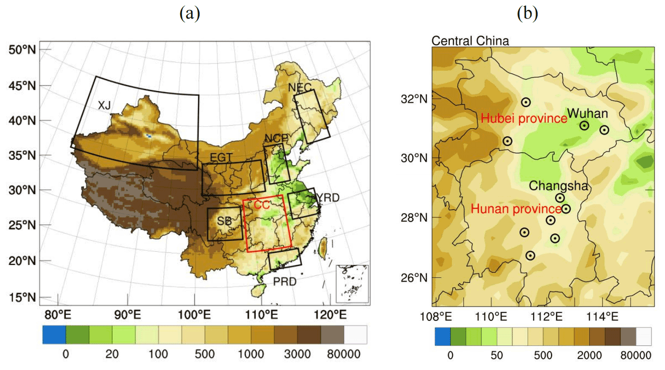
Figure 1 (a) Maps of the WRF modelling domain and (b) central China. The colour bars represent the terrain altitude. The black rectangles in (a) are North China Plain (NCP), northeastern China (NEC), Energy Golden Triangle (EGT), Xinjiang (XJ), Sichuan Basin (SB), Yangtze River Delta (YRD), and Pearl River Delta (PRD). The red rectangle in (a) represents central China (CC). (b) The details of CC. Black circle with dots in (b) represent the locations of large cities. The red characters in (b) are the name of provinces, and the black characters are the name of capital cities. Wuhan and Changsha are the capitals of Hubei and Hunan provinces. Inset in (a): South China Sea. Units: m.

Table 1 WRF–Chem model configuration.

2.2 4DVAR system

4DVAR is a continuous data assimilation method to simultaneously assimilate a time series of observations over a time window. It produces an analysis that fit a set of observations taken over the time window. The time evolution of the concerning quantities is governed using a deterministic model as a strong constraint. The cost function of 4DVAR can be written as follows:

$$\begin{array}{}\text{(1)}& \begin{array}{rl}J& ={\displaystyle \frac{\mathrm{1}}{\mathrm{2}}}{\left(c_{\mathrm{0}}-c_{\mathrm{0}}^{\mathrm{b}}\right)}^T{\mathbf{B}}_c^{-\mathrm{1}}\left(c_{\mathrm{0}}-c_{\mathrm{0}}^{\mathrm{b}}\right)\\ & +{\displaystyle \frac{\mathrm{1}}{\mathrm{2}}}{\sum }_{i=\mathrm{0}}^{n-\mathrm{1}}{\left(e_i-e_i^{\mathrm{b}}\right)}^T{\mathbf{B}}_{\mathrm{ei}}^{-\mathrm{1}}\left(e_i-e_i^{\mathrm{b}}\right)\\ & +{\displaystyle \frac{\mathrm{1}}{\mathrm{2}}}{\sum }_{i=\mathrm{0}}^n{\left(y_i^o-{\mathit{H}}_i{c}_i\right)}^T{\mathbf{R}}_{\mathrm{i}}^{-\mathrm{1}}\left(y_i^{\mathrm{o}}-{\mathit{H}}_i{c}_i\right),\end{array}\end{array}$$

where c₀ and e_i are the control variables to denote the initial concentration vector and the emission to estimate. $c_{\mathrm{0}}^{\mathrm{b}}$ is the background concentration at zero time, and $e_i^{\mathrm{b}}$ is the background emission. The subscripts of the variables represent time levels, and n is the time window. The first term in Eq. (1) is the background term due to the initial concentration field, and the second term is the background term for emissions in the time window. B_c and ${\mathbf{B}}_{{\mathrm{e}}_i}$ are the background error covariances (BECs) for the initial concentrations and background emissions. The third term is the observation term, where $y_i^{\mathrm{o}}$ is the observation vector at time i. H_i is the observation operator mapping the control variables to the observations, and R_i is the observation error covariance matrix. The concentration c_i is governed by a model.

$$\begin{array}{}\text{(2)}& c_i=f_{i,i-\mathrm{1}}\left(c_{i-\mathrm{1}},e_{i-\mathrm{1}}\right),\end{array}$$

where $f_{i,i-\mathrm{1}}$ represents the model time integration for one time step from time i−1 to i. The increment field of the initial SO₂ concentration can be written as $\mathit{\delta }{c}_{\mathrm{0}}=c_{\mathrm{0}}-c_{\mathrm{0}}^{\mathrm{b}}$, and the increment field of SO₂ emission as $\mathit{\delta }{e}_i=e_i-e_i^{\mathrm{b}}$. The innovation vector is denoted as $d_i\equiv y_i^{\mathrm{o}}-{\mathit{H}}_i\left(c_i\right)$, which is the difference between the observations and the model equivalent state. Thus, the cost function Eq. (1) can be written in an incremental form as follows:

$$\begin{array}{}\text{(3)}& \begin{array}{rl}J& ={\displaystyle \frac{\mathrm{1}}{\mathrm{2}}}{\left(\mathit{\delta }{c}_{\mathrm{0}}\right)}^T{\mathbf{B}}_{\mathrm{c}}^{-\mathrm{1}}\left(\mathit{\delta }{c}_{\mathrm{0}}\right)+{\displaystyle \frac{\mathrm{1}}{\mathrm{2}}}{\sum }_{i=\mathrm{0}}^{n-\mathrm{1}}{\left(\mathit{\delta }{e}_i\right)}^T{\mathbf{B}}_{{\mathrm{e}}_i}^{-\mathrm{1}}\left(\mathit{\delta }{e}_i\right)\\ & +{\displaystyle \frac{\mathrm{1}}{\mathrm{2}}}{\sum }_{i=\mathrm{0}}^n{\left(d_i-{\mathit{H}}_i\mathit{\delta }{c}_i\right)}^T{\mathbf{R}}_i^{-\mathrm{1}}\left(d_i-{\mathit{H}}_i\mathit{\delta }{c}_i\right).\end{array}\end{array}$$

Using a linearisation approximation, Eq. (2) becomes

$$\begin{array}{}\text{(4)}& \mathit{\delta }{c}_i=L_{i,i-\mathrm{1}}\mathit{\delta }{c}_{i-\mathrm{1}}+L_{i,i-\mathrm{1}}{\mathrm{\Gamma }}_{i-\mathrm{1}}\mathit{\delta }{e}_{i-\mathrm{1}},\end{array}$$

where $L_{i,i-\mathrm{1}}$ and Γ_i−1 are Jacobians of $f_{i,i-\mathrm{1}}$ with respect to δc_i−1 and δe_i−1, and $i=\mathrm{1},\mathrm{2},\mathrm{\dots }n$. Thus, with a time integration, Eq. (4) can be presented as

$$\begin{array}{}\text{(5)}& \mathit{\delta }{c}_i=L_{i,\mathrm{0}}\mathit{\delta }{c}_{\mathrm{0}}+{\sum }_{l=\mathrm{0}}^{i-\mathrm{1}}{L}_{i,l}{\mathrm{\Gamma }}_l\mathit{\delta }{e}_l,\end{array}$$

where L_i,0 denotes the tangent linear model operator of the CTM acting on δc₀, and the subscript is the time step from i to the initial time. L_i,lΓ_l ($l=\mathrm{0},\mathrm{1},\mathrm{\dots }i-\mathrm{1})$ is the operator acting on δe_l, and Γ_l is an operator that converts emissions to concentrations.

There are several numerical algorithms available to minimise the cost function in Eq. (3) (Courtier et al., 1994; Li and Navon, 2001). For the algorithms to minimise Eq. (3) with large dimensions, the gradient of the cost function is required. The gradient with respect to δc₀ and δe_i ($i=\mathrm{0},\mathrm{1},\mathrm{\dots },n-\mathrm{1})$ can be written as

$$\begin{array}{}\text{(6)}& {\displaystyle \frac{\partial J}{\partial \mathit{\delta }{c}_{\mathrm{0}}}}={\mathbf{B}}_{\mathrm{c}}^{-\mathrm{1}}\left(\mathit{\delta }{c}_{\mathrm{0}}\right)+{\sum }_{l=\mathrm{0}}^n{L}_{l,\mathrm{0}}^T{\mathit{H}}_l^T{\mathbf{R}}_l^{-\mathrm{1}}\left(d_l-{\mathit{H}}_l\mathit{\delta }{c}_l\right).\end{array}$$

$$\begin{array}{}\text{(7)}& \begin{array}{rl}{\displaystyle \frac{\partial J}{\partial \mathit{\delta }{e}_i}}& ={\mathbf{B}}_{{\mathrm{e}}_i}^{-\mathrm{1}}\left(\mathit{\delta }{e}_i\right)+{\sum }_{l=\mathrm{i}+\mathrm{1}}^n{\mathrm{\Gamma }}_i^T{L}_{l,\mathrm{i}}^T{\mathit{H}}_l^T{\mathbf{R}}_l^{-\mathrm{1}}\\ & \left(d_l-{\mathit{H}}_l\mathit{\delta }{c}_l\right)(i=\mathrm{0},\mathrm{1},\mathrm{\dots },n-\mathrm{1}).\end{array}\end{array}$$

Here, $L_{\mathrm{0},\mathrm{0}}=I$ for i=0, where I is an identity matrix. A time window of 6 h is typically used in operational synoptic-scale numerical weather predictions. Since a SO₂ lifetime in a model grid is usually less than 6 h (Fioletov et al., 2015), we still use a window of 6 h (n=6) in the experiments presented in the following sections.

Equations (6) and (7) include three types of adjoint operators, that is, Γ^TL^T and H^T, which are derived from the tangent linear model operator ΓL, and observation operator H, respectively. The tangent linear operators Γ and L from WRF–Chem are very complex and computationally demanding, we simplify the CTM to focus on SO₂.

WRF–Chem is an online coupled air quality model with sophisticated and comprehensive physical and chemical processes. Focusing on SO₂, the governing equation for the concentration can be written as

$$\begin{array}{}\text{(8)}& \begin{array}{rl}{\displaystyle \frac{\partial c}{\partial t}}& =-u{\displaystyle \frac{\partial c}{\partial x}}-v{\displaystyle \frac{\partial c}{\partial y}}-w{\displaystyle \frac{\partial c}{\partial z}}+{\displaystyle \frac{\partial }{\partial x}}\left(K_x{\displaystyle \frac{\partial c}{\partial x}}\right)\\ & +{\displaystyle \frac{\partial }{\partial y}}\left(K_y{\displaystyle \frac{\partial c}{\partial y}}\right)+{\displaystyle \frac{\partial }{\partial z}}\left(K_z{\displaystyle \frac{\partial c}{\partial z}}\right)-e^{-\mathrm{\Lambda }}{\displaystyle \frac{\partial c}{\partial t}}\\ & -r{\displaystyle \frac{\partial c}{\partial t}}+V_{\mathrm{m}}{\displaystyle \frac{{\mathit{\rho }}_{\mathrm{air}}}{\mathit{\rho }}}{\displaystyle \frac{\mathrm{\Delta }S}{\mathrm{d}z}}e,\end{array}\end{array}$$

where c is the gas/aerosol concentration, and u, v, and w denote the wind in x, y, and z directions, respectively. Thus, the $u\frac{\partial c}{\mathrm{d}x}+v\frac{\partial c}{\mathrm{d}y}+w\frac{\partial c}{\mathrm{d}z}$ is a transport term. K_x, K_y, and K_z are turbulent exchange coefficients in x, y, and z directions, respectively, based on K theory of turbulence, and $\frac{\partial }{\partial x}\left(K_x\frac{\partial c}{\partial x}\right)+\frac{\partial }{\partial y}\left(K_y\frac{\partial c}{\partial y}\right)+\frac{\partial }{\partial z}\left(K_z\frac{\partial c}{\partial z}\right)$ is the turbulent term. In the study, the horizontal grid spacing is 27 km, thus the $\frac{\partial }{\partial x}\left(K_x\frac{\partial c}{\partial x}\right)+\frac{\partial }{\partial y}\left(K_y\frac{\partial c}{\partial y}\right)$ can be neglected. But the vertical turbulence term $\left(\frac{\partial }{\partial z}\left(K_z\frac{\partial c}{\partial z}\right)\right)$ should be retained since the vertical grid spacing is generally less 200 m in the lower and middle layers. $e^{-\mathrm{\Lambda }}\frac{\partial c}{\partial t}$ denotes the wet deposition term, where Λ is the loss rate (Grell and Dévényi, 2002) and e is the base of natural logarithms (=0.272), $r\frac{\partial c}{\partial t}$ is the chemical term, where r is the chemical reaction rate of the species, and $V_{\mathrm{m}}\frac{{\mathit{\rho }}_{\mathrm{air}}}{\mathit{\rho }}\frac{\mathrm{\Delta }S}{\mathrm{d}z}e$ is the emission term, where e denotes the emission source of the species. $V_{\mathrm{m}}=\mathrm{22.4}\times {\mathrm{10}}^{-\mathrm{3}}$ m³ mol⁻¹ is the molar gas volume, ρ is the air density of the actual atmosphere (kg m⁻³), ρ_air is the standard air density indicating the molar volume, and ΔS is the grid area.

From the simplified Eq. (8), the model operators of Γ and L can be written as

$$\begin{array}{}\text{(9)}& \begin{array}{rl}L& =-u{\displaystyle \frac{\partial c}{\partial x}}-v{\displaystyle \frac{\partial c}{\partial y}}-w{\displaystyle \frac{\partial c}{\partial z}}+{\displaystyle \frac{\partial }{\partial z}}\left(K_z{\displaystyle \frac{\partial c}{\partial z}}\right)\\ & -e^{-\mathrm{\Lambda }}{\displaystyle \frac{\partial c}{\partial t}}-r{\displaystyle \frac{\partial c}{\partial t}}.\end{array}\end{array}$$

$$\begin{array}{}\text{(10)}& \mathrm{\Gamma }=V_{\mathrm{m}}{\displaystyle \frac{{\mathit{\rho }}_{\mathrm{air}}}{\mathit{\rho }}}{\displaystyle \frac{\mathrm{\Delta }S}{\mathrm{d}z}}e.\end{array}$$

Using tangent linear coding techniques, we could derive the code for the discretised tangent linear operators L and Γ (Eqs. 9–10) from the source code built in WRF–Chem. Once the source code is available for the tangent linear operators, we use the adjoint coding technique to derive the adjoint operator. The adjoint coding technique are detailed in Hoffman et al. (1992).

2.3 Observational and background error covariances

R_i in Eq. (1) is the observational error covariance for a set of observations (y_i), where B_c and ${\mathbf{B}}_{{\mathrm{e}}_i}$ are the BECs for the concentrations and emissions, respectively. In a DA system, R_i and BEC play important roles in successful assimilation. The observational errors include the measurement error (observed value error) and representative error (error of observation operator H). The observation error ${\mathit{\epsilon }}_{{\mathrm{SO}}_{\mathrm{2}}}$ is defined as below:

$$\begin{array}{}\text{(11)}& {\mathit{\epsilon }}_{{\mathrm{SO}}_{\mathrm{2}}}=\sqrt{{\mathit{\epsilon }}_{\mathrm{r}}^{\mathrm{2}}+{\mathit{\epsilon }}_o^{\mathrm{2}}},\end{array}$$

where ε_o is the measurement error, and ε_r is the representative error. The measurement error ε_o is the systematic error generated during monitoring by the instrument at each environmental monitoring station. Therefore, the measurement error ε_o of SO₂ observation in this study is 1.0 µg m⁻³, similar to that reported by Chen et al. (2019).

The representative error ε_r is caused by converting the model variable to the observation variable (Schwartz et al., 2012) and can be expressed as

$$\begin{array}{}\text{(12)}& {\mathit{\epsilon }}_{\mathrm{r}}=\mathit{\gamma }{\mathit{\epsilon }}_o\sqrt{{\displaystyle \frac{\mathrm{d}x}{L}}},\end{array}$$

where γ is an adjustable parameter scaling ε_o. γ=0.5 was used in accordance with that used in Dai et al. (2021). Furthermore, dx is the grid spacing (27 km in this study) and L is the radius of influence of an observation, which was taken as 2 km according to that reported by Chen et al. (2019). Then, ε_r=1.8 µg m⁻³ is calculated from Eq. (12).

BECs (B_c and ${\mathbf{B}}_{{\mathrm{e}}_i}$ in Eq. 1) are the error covariance matrices of SO₂ concentrations and emissions. Practically, the BEC is overly large for handling numerically. Thus, we followed the method used by Li et al. (2013) and Zang et al. (2016) to simplify B:

$$\begin{array}{}\text{(13)}& \mathbf{B}=\mathbf{D}\mathbf{C}{\mathbf{D}}^T,\end{array}$$

where D is the RMSE matrix and C is the correlation matrix.

C can be simplified by the Cholesky factorisation and Kronecker product method (Li et al., 2013) as

$$\begin{array}{}\text{(14)}& {\mathbf{C}}^{\frac{\mathrm{1}}{\mathrm{2}}}={\mathbf{C}}_x^{\frac{\mathrm{1}}{\mathrm{2}}}\otimes {\mathbf{C}}_y^{\frac{\mathrm{1}}{\mathrm{2}}}\otimes {\mathbf{C}}_z^{\frac{\mathrm{1}}{\mathrm{2}}}.\end{array}$$

For ${\mathbf{B}}_{{\mathrm{e}}_{\mathrm{i}}}$, the standard deviation ${\mathbf{D}}_{{\mathrm{e}}_{\mathrm{i}}}$ is diagonal with a 200 % error (Wang et al., 2012) and ${\mathbf{C}}_{{\mathrm{e}}_i}$ is a block diagonal matrix, with the main diagonal blocks being the correlation matrices of SO₂ emission. The main diagonal blocks of ${\mathbf{C}}_{{\mathrm{e}}_i}$ is 1.0 because the emission in each grid point is independent of that in other grids.

The National Meteorological Center method (Parrish and Derber, 1992) was used to estimate the BEC of SO₂ concentrations. The differences between 48 and 24 h forecasts were generated from 17 January to 18 February 2020. The first initial chemical field at 00:00 UTC on 17 January 2020 was obtained from a 10 d forecast in consideration of spin-up. The subsequent initial chemical fields were derived from the former forecast 1 d prior. The horizontal length scale was used to determine the magnitude of SO₂ variance in the horizontal direction. This scale can be estimated by the curve of the horizontal correlation with distances, and the horizontal correlation is approximately expressed by a Gaussian function $e^{\frac{(x\mathrm{1}-x{)}^{\mathrm{2}}}{\mathrm{2}{L}_{\mathrm{s}}^{\mathrm{2}}}}$ (e is the base of natural logarithms equal to 0.272). Here, x1 and x are two points, and L_s is the horizontal length scale. According to Zang et al. (2016), when the intersection of the decline curve reaches $e^{\mathrm{1}/\mathrm{2}}$, the distance can be approximated as the horizontal length scale in Fig. 2a. The horizontal length scale was 81 km in this study. The vertical variance of SO₂ concentrations was considered by the vertical correlations in the BEC. A strong relationship was observed in the boundary layer (approximately below the 20th model layer) in the vertical direction (Fig. 2b). The standard deviation demonstrates the reliability of the forecasting model, and the standard deviation for the vertical distribution of SO₂ concentrations decreased with increasing height in the B_c (Fig. 2c).

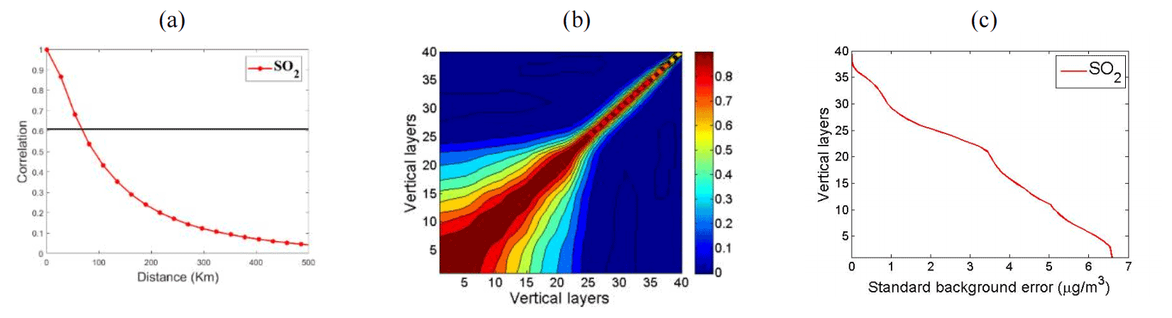
Figure 2 Background error covariation of SO₂ concentrations. (a) Vertical distribution of the horizontal correlation; the horizontal thin black line is the reference line ($e^{\mathrm{1}/\mathrm{2}}$) used to determine the horizontal correlation scales. (b) Vertical correlations. (c) Vertical distribution of the standard deviation.

2.4 Observation and emission data

Hourly SO₂ data obtained from the website of the China National Environmental Monitoring Center (http://www.cnemc.cn/en/, last access: 28 September 2022) were used for assimilation and evaluation. There were 1933 stations in China in January 2020. Most observational stations were located in central and eastern China, whereas the stations in the west were relatively sparse. The sites were gridded into the model grid (27×27 km²). If more than two stations were in the same grid, one station was randomly selected to verify the improvements relating to using optimised emissions, and the remaining sites were used for assimilation. In this study, 508 sites were selected for verification, and the remaining 1425 stations were used for assimilation. A strict criterion was used to remove SO₂ observations with values exceeding 650 µg m⁻³ to ensure data quality (Chen et al., 2019).

The background anthropogenic emissions data were obtained from the MEIC (http://www.meicmodel.org/, last access: 28 September 2022) developed by Tsinghua University, with a $\mathrm{0.25}{}^{\circ }\times \mathrm{0.25}{}^{\circ }$ resolution and 2016 as the base year. The MEIC is a “bottom-up” emission inventory that covers 31 provinces on the Chinese mainland, and includes eight major chemical species (Zhang et al., 2009), and counts anthropogenic emissions from sources in five sectors (power, industry, residential, transportation, and agriculture). Details of the technology-based approach and source classifications have been reported by Zhang et al. (2009). The actual emission inventory ($\mathrm{0.25}{}^{\circ }\times \mathrm{0.25}{}^{\circ }$) was pre-processed to match the model grid spacing (27 km).

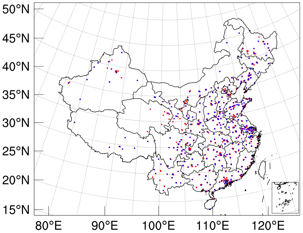
Figure 3 The locations of the 1425 SO₂ assimilated and 508 independent verification observation stations of the CNEMC are shown by the red and black dots, respectively. Inset: South China Sea.

2.5 Experimental design

Figure 4 shows a flowchart of the procedure used to optimise SO₂ emissions in a single time step of i. First, a forecast was performed using the WRF–Chem model and background emissions to generate the meteorological and chemical fields, which were recorded every 10 min and then used in the 4DVAR system. Then, the 4DVAR system performed every 6 h to obtain SO₂-optimised emissions and initial concentrations by assimilating the hourly SO₂ observations. For example, the observations during 00:00–06:00 UTC were assimilated using Eq. (1). The assimilated SO₂ concentration initial field (00:00 UTC) and the optimised SO₂ emissions during 00:00–05:00 UTC were obtained.

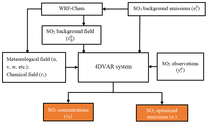
Figure 4 Flow chart of the SO₂ emissions optimisation procedure in a single time step of i. The orange boxes represent the SO₂-optimised emissions and SO₂ concentrations of output. The $c_{\mathrm{0}}^{\mathrm{b}}$, c₀, $e_i^{\mathrm{b}}$, e_i, and ${\mathrm{y}}_i^{\mathrm{o}}$ are the mathematical symbols from Eq. (1).

The SO₂ emissions during the COVID-19 lockdown over China were optimised to evaluate the performance of the 4DVAR system, and to analyse the reduction of SO₂ emissions related to the COVID-19 lockdown. The national lockdown was imposed in Wuhan and surrounding cities of Hubei provinces on 23 and 24 January 2020, respectively. Then, the Chinese mainland implemented the national lockdown policies on 26 January 2020. We selected the study period from 17 January to 6 February 2020, which covered the time before and during lockdown. The latest available MEIC emission inventory is based on the statistics of 2016. However, the changes of emissions between 2020 and 2016 are both related to the emissions reduction policies and COVID-19 lockdown. The difference between 2019 and 2020 emissions during the same period reflected the influence of COVID-19 lockdown on SO₂ emissions. Thus, the SO₂ emissions during the study period in 2019 was also optimised.

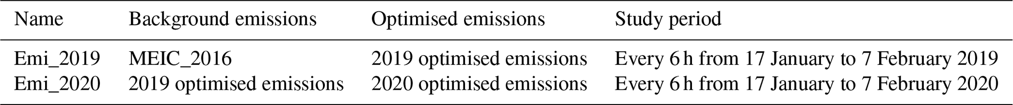
Table 2 summarises the details of DA emissions experiments. For the set of Emi_2019 experiments, the first DA process started on 17 January 2019, and the observations during 00:00–06:00 UTC of 17 January 2019 were assimilated by the 4DVAR system. Then, the optimised initial SO₂ concentration field (00:00 UTC) and SO₂ emissions during 00:00–05:00 UTC were obtained. Before conducting Emi_2019 experiment, 24 h forecasts were performed by WRF–Chem with MEIC_2016 emissions every 00:00 UTC from 17 January to 7 February 2019 to provide the physical and chemical parameters. The daily chemical initial conditions were obtained from the 24 h forecast of the previous day. For the 24 h forecast, the meteorological initial and boundary conditions were provided by the $\mathrm{1}{}^{\circ }\times \mathrm{1}{}^{\circ }$ National Centers for Environmental Prediction (NCEP) global final analysis data at a 6 h frequency. The chemical boundary fields were not considered because the domain used in this study was wider than that in China. For the Emi_2019 experiment, the emissions of 2019 were optimised by the 4DVAR system every 6 h with the background emissions of MEIC_2016. The physical and chemical parameters used in this DA process were obtained from the WRF–Chem forecast. For the Emi_2020 experiment, the DA process settings were similar to those of the Emi_2019 experiment. The optimised emissions for 2020 were obtained with the emission 2019 as background emission.

Table 2 Details of 4DVAR experiments to optimise emissions for 2019 and 2020.

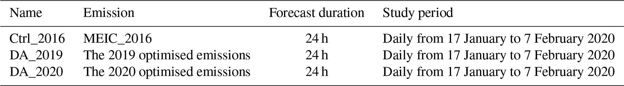
To estimate the improvement of SO₂ forecasts using optimised emissions, three sets of forecast experiments were performed using the MEIC_2016 emissions and the optimised emissions for 2019 and 2020, respectively, labelled Ctr_2016, DA_2019, and DA_2020, respectively (see Table 3). The three experiments were run daily with 24 h forecasts from 17 January to 7 February 2020 using the same WRF–Chem domain settings and physiochemical parameters. The SO₂ initial condition (IC) at 00:00 UTC on 17 January was based on the spin-up forecasts initialised at 00:00 UTC on 7 January 2020 for all three forecast experiments. The SO₂ ICs were later obtained from the 24 h forecast of the previous day for the three experiments, respectively. For example, the SO₂ IC of the experiment beginning at 00:00 UTC on 18 January was taken from the 24 h forecast result of the experiment beginning at 00:00 UTC of 17 January, and so on. Meteorological initial and boundary conditions were provided by the $\mathrm{1}{}^{\circ }\times \mathrm{1}{}^{\circ }$ NCEP global final analysis data at a 6 h frequency. The chemical boundary fields were not considered.

Table 3 Details of the forecast experiments using emissions from 2016, 2019, and 2020.

3 Results

3.1 Results of 4DVAR emission experiments

3.1.1 4DVAR test case

The first day (17 January 2019) was used as a test case to determine the effectiveness of using 4DVAR. The experiment employed MEIC_2016 as the background emissions and assimilated the hourly surface SO₂ observations during 00:00–06:00 UTC of 17 January 2019. The observed SO₂ concentrations in Fig. 5a indicated the heavy polluted areas with SO₂ concentrations exceeding 80 µg m⁻³ were mostly located in the North China Plain and northeast China. The areas lightly polluted with SO₂ concentrations below 40 µg m⁻³ were mostly located in southern China. Compared with the observed concentrations, the background concentrations (Fig. 5b) were underestimated in North China Plain and northeast China but overestimated in central China and the Sichuan Basin. Figure 5c shows the increment field of SO₂ concentrations (analysed field minus background field). Positive values in most of northern China and negative in central China and the Sichuan Basin were observed, suggesting that the optimised IC is more consistent with the observed SO₂ concentrations than the background concentrations. The evaluations of the optimised IC and background concentrations are shown in Fig. 5d. Compared with the background field, the mean bias in analysis field improved from −2.76 to 1.79 µg m⁻³ and RMSE decreased from 23.12 to 11.81 µg m⁻³, and the correlation coefficient (CORR) of analysis field increased from 0.19 to 0.84. The result indicates that the accuracy of the ICs of SO₂ concentrations were improved after using the 4DVAR method. The forecast accuracy can be improved using optimised ICs (Peng et al., 2017, 2018), but the emission is the most important factor influencing the forecast accuracy. The emissions and IC concentrations were simultaneously optimised in the EMI_2019 experiment using our 4DVAR system.

Figure 5 Simulated and observed SO₂ concentrations at 00:00 UTC, 17 January 2019. (a) Observations, (b) background concentrations, (c) SO₂ concentrations increment, (d) scatter plots, (e) background emissions, and (f) SO₂ emissions increment. Units: µg m⁻³ for (a)–(d), and mol km⁻² h⁻¹ for (e) and (f). Insets: South China Sea.

Figure 5e presents the background emission of MEIC_2016 at 00:00 UTC. According to Fig. 5a and b, MEIC_2016 emissions underestimated in most of northern China and overestimated in central China and Sichuan Basin. Figure 5f shows the increment of SO₂ emissions at 00:00 UTC 17 January 2019 by using the 4DVAR system. There were positive increment in North China Plain and northeast China, and negative increment in central China and Sichuan Basin. The distribution of the incremental SO₂ emissions was consistent with that of the incremental SO₂ concentration (Fig. 5c). There is a reasonable relationship between the two increments since the underestimated/overestimated emission may result in underestimated/overestimated simulation of concentration.

3.1.2 Spatial distribution of emissions

Compared with MEIC_2016 (Fig. 6a), the emissions for 2019 and 2020 (Fig. 6b and c) from the 4DVAR experiments of Emi_2019 and Emi_2020 decreased in the area with heavy emissions, particularly in North China Plain and central China. The reduction in emissions between 2019 and MEIC_2016 may primarily result from the national pollution control policy. However, the reduction of emissions between 2020 and 2019 may primarily result from the COVID 2019 lockdown, including school and workplace closures, event and public gathering cancellation, and restrictions on public transport.

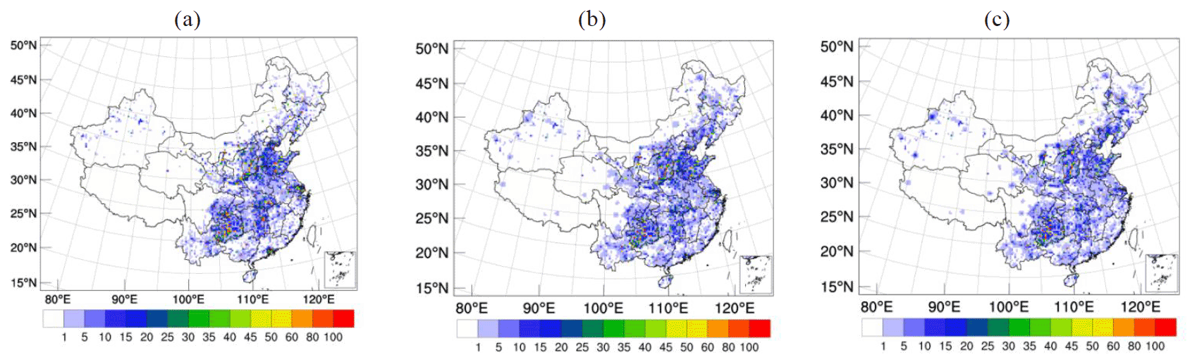
Figure 6 Emissions in China for (a) MEIC_2016, (b) 2019, and (c) 2020. Units: mol km⁻² h⁻¹. Insets: South China Sea.

Figure 7a shows the difference in emissions between 2020 and 2019. The negative values were seen in most of the areas with strict lockdown, such as North China Plain, central China, Yangtze River Delta, and Pearl River Delta. It indicates that the 2020 emission substantially decrease, compared with the 2019 emission due to the COVID-19 lockdown. The reducing ratio of emission was averaged in China as 9.2 % (Fig. 7b), but over 40.0 % in most areas of north China and central China. Zheng et al. (2021) have found that SO₂ emissions in China decreased by 12.0 % in January and February 2020 compared to values in 2019. Fan et al. (2020) have also reported the SO₂ concentration decreased by 20.0 %–50.0 % over China during the COVID-19 lockdown period in the spring of 2020 based on TROPOMI satellite data. Our results are similar to those of previous studies. In addition, SO₂ emissions increased in some areas of northeast China, Tibetan Plateau, Yunnan province, and the southeast coastal areas, where the epidemic was weaker than that in other areas (Kraemer et al., 2020; Tian et al., 2020). Most of the increase in SO₂ was <10 mol km⁻² h⁻¹, but the positive ratios were >100.0 %, suggesting that new emission sources were generated. It is suggested that these newly generated emissions were probably due to relocating power plants and factories from cities to the surrounding villages (Chen et al., 2019).

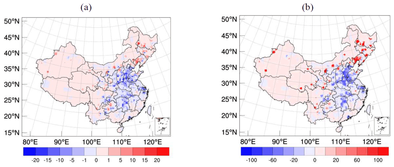
Figure 7 (a) Difference between 2020 and 2019 emissions, and (b) ratios of (2020–2019)$/\mathrm{2019}$ emissions in China. Units are mol km⁻² h⁻¹ for (a) and percent (%) for (b). Insets: South China Sea.

Figure 8 shows the similar analyses as in Fig. 6, but for central China. Wuhan first implemented the first-level response to COVID-19 with strict lockdown policies on 23 January 2020, and the entire Hubei province implemented lockdown on 24 January 2020. The heavy emissions exceeding 20.0 mol km⁻² h⁻¹ were most located around large cities from the emissions of 2019 and 2020 (Fig. 8b and c). Figure 9a shows the difference between 2020 and 2019 emissions in central China. The average emission value in Wuhan was 43.0 mol km⁻² h⁻¹ in 2019 and 34.0 mol km⁻² h⁻¹ in 2020, showing a reduction of 21.0 % compared with the emissions for 2019. Al-qaness et al. (2021) have also found approximately 15 % decrease in SO₂ concentrations with 15 % around Wuhan. Furthermore, almost all emissions around the large cities decreased by 5–10 mol km⁻² h⁻¹ (Fig. 9a), and the negative ratios were >20.0 % (Fig. 9b). The large reduction in SO₂ emissions were related to the decrease in industrial and domestic coal combustion and power plants during the COVID-19 lockdown (Zheng et al., 2018, 2021; Bian et al., 2019; van der A et al., 2017).

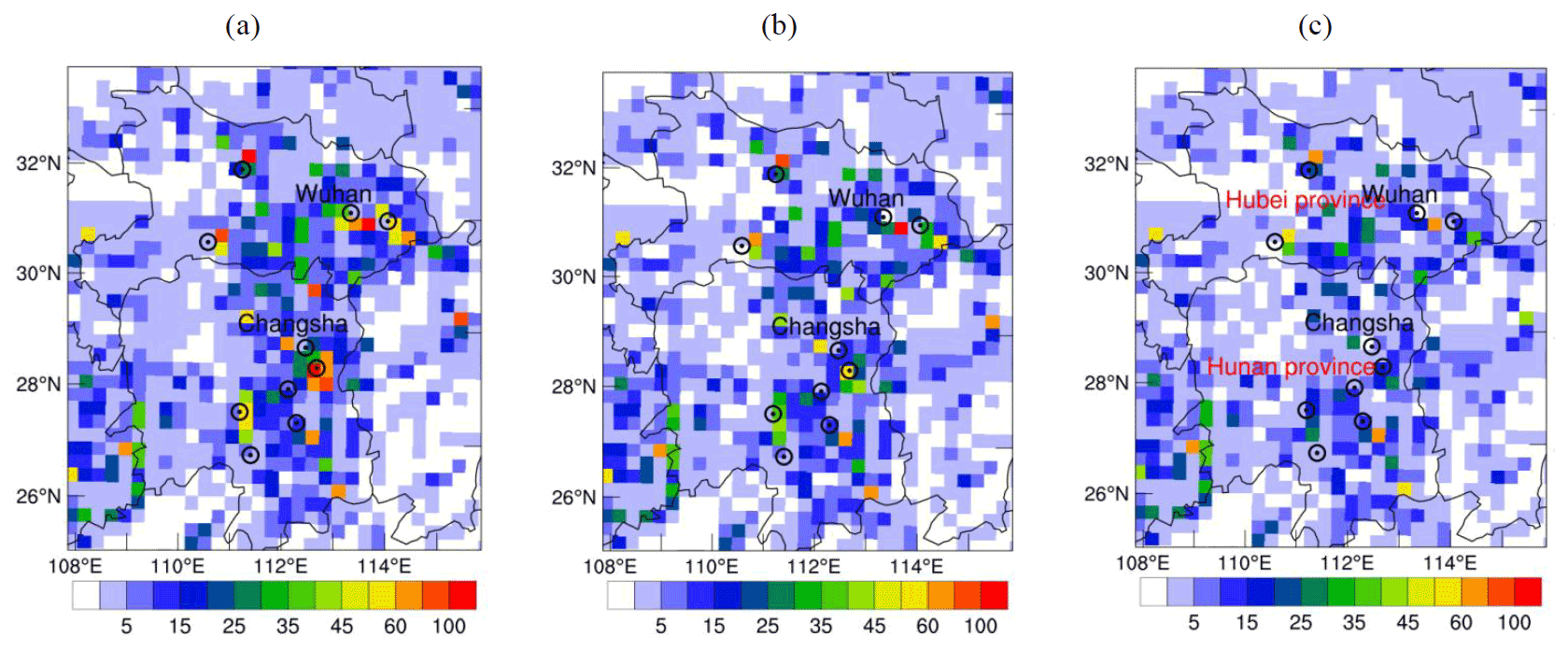
Figure 8 Emissions in central China for (a) MEIC_2016, (b) 2019, and (c) 2020. Black circles with dots are the locations of large cities. The red characters in (c) are the name of provinces, and the black characters are the name of cities. Wuhan and Changsha are the capitals of Hubei and Hunan provinces, respectively. Unit: mol km⁻² h⁻¹.

Figure 9 (a) Difference between 2020 and 2019 emissions, and (b) ratios of (2020–2019)$/\mathrm{2019}$ emissions in central China. Black circles with dots are the location of large cities. The red characters are the name of provinces, and the black characters are the name of cities. Wuhan and Changsha are the capitals of Hubei and Hunan provinces, respectively. Units: mol km⁻² h⁻¹ for (a) and percent (%) for (b).

3.1.3 Temporal evolution of emissions

Figure 10 shows the daily SO₂ emissions for MEIC_2016, Emi_2019, and Emi_2020 over all grid points. The average emissions in the Chinese mainland (Fig. 10a) from MEIC_2016, Emi_2019, and Emi_2020 were 42.2×10⁶, 40.1×10⁶, and 36.4×10⁶ kg d⁻¹ during the same period from 17 January to 7 February. The emissions for 2020 decreased by 9.2 % compared with those for 2019, indicating a decrease between 2020 and 2019 due to the COVID-19-related lockdown. In Emi_2019 emissions, the lowest emissions occurred on 1 February 2019, but increased during 4–6 February 2019, mainly attributed to the traditional firework displays during Spring Festival (Wang et al., 2007; Zhang et al., 2020; Huang et al., 2021a). Complex changes in SO₂ emission trends were observed in 2020 in relation to reduced human activity. For example, a peak of 40.1×10⁶ kg d⁻¹ occurred on 24 January 2020, in relation to firework displays (Fig. 10a), after which the SO₂ emissions decreased because of the COVID-19 lockdown. For central China, the average SO₂ emissions were 5.7×10⁶, 4.2×10⁶ and 3.1×10⁶ kg d⁻¹ during the same period from 17 January to 7 February (Fig. 10b). The SO₂ emissions peaked at 3.5×10⁶ kg d⁻¹ on 24 January 2020 due to firework displays, and a reduction began from 26 January 2020 because of the national lockdown.

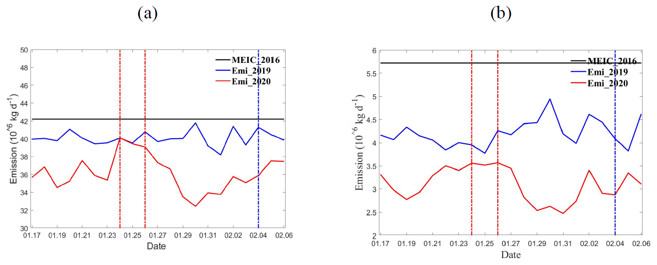
Figure 10 Time series of daily SO₂ emissions in (a) China and (b) central China. The red dotted lines represent the dates of the start of national lockdown and the Chinese Spring Festival in 2020. The blue dotted line represents the Chinese Spring Festival in 2019. Units: 10⁶ kg d⁻¹.

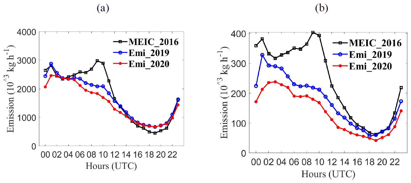
Figure 11 shows the average hourly emissions for MEIC_2016, Emi_2019, and Emi_2020 emissions from 17 January to 7 February over all grid points. The hourly factors for MEIC_2016 were obtained from power plant report, with two peaks during the day at 01:00 UTC (09:00 BJ time – Beijing time) and 09:00 UTC (17:00 BJ time) to reflect the emissions at rush hours (Chen et al., 2019; Hu et al., 2022). In the Chinese mainland (Fig. 11a), the emissions of 2019 and 2020 were lower than those of MEIC_2016 during 06:00–12:00 UTC. This is primarily due to the recent implementation of China's emission reduction policies and the COVID-19 lockdown. Previous studies have shown that the second peak (09:00 UTC) of SO₂ emissions had weakened (Chen et al., 2019), which was also reflected in our hourly emission analysis. The emissions for Emi_2019 and Emi_2020 were higher than those of MEIC_2016 during 16:00–20:00 UTC, but remain almost unchanged between Emi_2019 and Emi_2020 emissions. During this time period, most factories were closed and human activities were reduced. The SO₂ emissions are primarily emitted from power plants, and the changes in emissions are small between different years (Zheng et al., 2018, 2021; Hu et al., 2022). Thus, the increase in Emi_2019 and Emi_2020 emissions during 16:00–20:00 UTC are mainly due to the uncertainties of MEIC_2016 (Chen et al., 2019). Compared with the average emissions for Emi_2019, those for Emi_2020 emissions decreased by 18.0 %, reflecting the reduction due to the COVID-19 lockdown. The emissions in 2019 and 2020 in central China were lower than those in MEIC_2016 for 24 h period, with a maximum reduction at 09:00 UTC (Fig. 9b). Compared with the emissions in 2019, the emissions in 2020 appreciably decreased by 22.3 %–42.1 %. The first peak of the emissions in 2020 was delayed and occurred at 02:00 UTC because of the national lockdown policies. The most substantial reduction between 2019 and 2020 emissions was $-\mathrm{120.4}\times {\mathrm{10}}^{\mathrm{3}}$ kg h⁻¹ at 01:00 UTC, reflecting the change in human activities at the first peak. Additionally, although there was only a moderate decrease in SO₂ emissions ($-\mathrm{72.3}\times {\mathrm{10}}^{\mathrm{3}}$ kg h⁻¹) at 13:00 UTC, the reduction ratio (−54.5 %) was the largest during 24 h.

Figure 11 Hourly emissions for (a) China and (b) central China (unit: 10³ kg h⁻¹).

3.2 Results of forecast experiments

Using the emissions of MEIC_2016, Emi_2019, and Emi_2020, three forecast experiments (Ctrl_2016, DA_2019, and DA_2020 in Table 3) were implemented to further demonstrate the effect of optimised emissions. Figure 12 shows the average 24 h forecast of SO₂ concentrations of the three forecast experiments over all stations in China during the study period from 17 January to 7 February 2020. The DA_2020 experiment with the 2020 emissions performed much better than the Ctrl_2016 and DA_2019 experiments, indicating that the emission is one of the most important factors for 24 h forecasts. The SO₂ concentrations in Ctrl_2016 and DA_2019 were overestimated, particularly during 08:00–18:00 UTC (Fig. 12a), while the SO₂ concentrations in DA_2020 are similar to the observed concentrations. The result showed the 4DVAR system effectively optimises emissions and improves the accuracy of forecasts. The average RMSEs of the three experiments were 21.7, 15.6, and 10.7 µg m⁻³, respectively. Compared to the average RMSE of Ctrl_2016 experiment, the RMSEs of the DA_2019 and DA_2020 decreased by 28.1 % and 50.7 %. The average CORRs for the Ctrl_2016, DA_2019, and DA_2020 experiments were 0.20, 0.38, and 0.61, respectively. Thus, the average CORRs for DA_2019 and DA_2020 experiments increased by 89.5 % and 205.9 % from the CORR for Ctrl_2016 experiment. The average bias of Ctrl_2016, DA_ 2019, and DA_2020 experiments were 5.9, 4.9, and −0.1 µg m⁻³, respectively. It is suggested that the optimised emissions could substantially improve forecast accuracy, and the 4DVAR approach is effective to optimise daily and hourly emissions during an accidental special event.

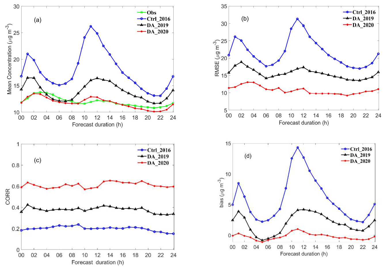
Figure 12 Forecast accuracy of SO₂ concentrations in China for the Ctrl_2016, DA_2019, and DA_2020 experiments during the study period in 2020: (a) mean concentration, (b) RMSE, (c) CORR, and (d) bias. Unit: µg m⁻³ for (a), (b), and (d). Obs: observation.

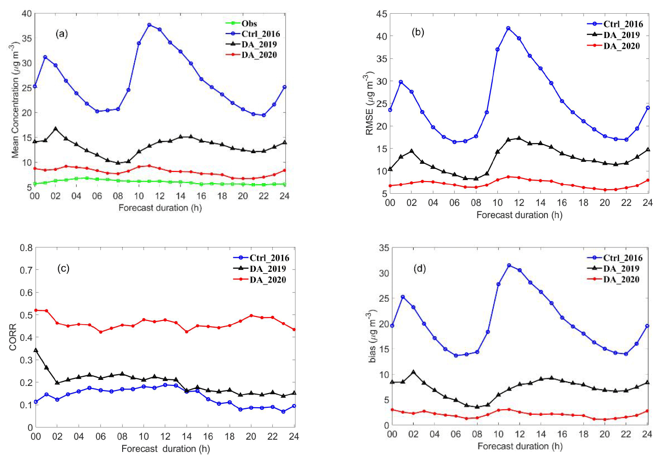
Figure 13 Forecast accuracy of SO₂ concentrations in central China using the Ctrl_2016, DA_2019, and DA_2020 experiments during the study period in 2020. (a) Mean concentration, (b) root mean square error (RMSE), (c) correlation coefficient (CORR), and (d) bias. Unit: µg m⁻³ for (a), (b), and (d). Obs: observation.

Figure 13 shows the same analyses as those presented in Fig. 12, but for central China. It also showed that the forecast accuracies of the DA_2019 and DA_2020 experiments were higher than those of Ctrl_2016. The average observation concentration was <10 µg m⁻³, which is substantially lower than that for Chinese mainland (Fig. 12a). The mean concentration of DA_2020 was close to the observed concentration in central China. The above results suggest that although the 2020 optimised emissions were generally consistent with the real emissions, they were slightly higher than the real emissions. In the 4DVAR optimisation process, each grid will be influenced by surrounding grids because of the advection and vertical mixing. The theory of 4DVAR method is to take a balance between the observations and background field, and to obtain the optimised field. Therefore, when the observations are lower and the background fields are higher, the value of the optimised field will be higher than the observation. Compared to that of Ctrl_2016, the average bias of the DA_2019 and DA_2020 experiments decreased from 20.1 to 12.6 and 3.5 µg m⁻³. The average RMSE decreased by 48.8 % and 77.0 %, and the average CORR increased by 44.3 % and 238.7 %. This indicates that the forecast accuracy substantially improved after using optimised emissions.

4 Conclusions

In this study, we developed a 4DVAR system based on the WRF–Chem model to estimate SO₂ emissions, where the initial SO₂ concentration and emissions were set as the state variables to estimate SO₂ emissions. An adjoint operator was derived from the WRF–Chem model, focusing on the processes of transport, dry/wet deposition, vertical turbulence, and SO₂ chemical reactions. Hourly SO₂ concentration observations were assimilated to optimise SO₂ emissions, which were used to improve the SO₂ forecasting accuracy.

The 4DVAR system was applied to investigate SO₂ emission changes during the COVID-19 lockdown in China, particularly focusing on central China. The MEIC_2016 emissions were set as the background values. The average emissions of MEIC_2016, 2019, and 2020 were 42.2×10⁶, 40.1×10⁶, and 36.4×10⁶ kg d⁻¹, namely 2020 emissions decreased by 9.2 % compared with those in 2019, indicating a substantial decrease between 2019 and 2020 due to the COVID-19 related lockdown. The average 2020 emissions in central China dropped by 21.0 % compared to the 2019 emissions, owing to the strict lockdown policy during COVID-19. The largest decrease in emissions occurred in Wuhan (decline of 57.0 %), which COVID-19 had heavily affected by this time. Hourly average emissions were analysed to estimate the changes between 2019 and 2020. Compared with 2019 emissions, the average 2020 emissions decreased by 18.0 %, reflecting lockdown-associated reduction in SO₂ emissions. The 2020 emissions in central China decreased by 22.3 %–42.1 % compared with the 2019 emissions.

Three sets of forecast experiments for 2020, using MEIC_2016, Emi_2019, and Emi_2020 emissions, were conducted to illustrate the effects of the optimised emissions. The experiment with MEIC_2016 emissions overestimated the SO₂ concentration forecast, whereas the experiment with 2019 optimised emissions decreased the concentrations but still overestimated the values. The forecast accuracy of the experiment with the 2020 emissions was the closest to the observation. The RMSE of the experiments with the emissions in 2019 and 2020 decreased from 21.7 to 15.6, and 10.7 µg m⁻³, respectively, and the correlation coefficient increased from 0.20 to 0.38 and 0.61, respectively, compared with those of the experiment with MEIC_2016 emissions. For central China, the average RMSE and correlation coefficient of the experiment with MEIC_2016 were 24.6 µg m⁻³ and 0.1. Compared with the average RMSE of the experiment with MEIC_2016, those of the experiments with 2019 and 2020 emissions decreased by 48.8 % and 77.0 %, and the average correlation coefficient increased by 44.3 % and 238.7 %.

Though our 4DVAR system could effectively optimise real time emission as a “top-down” approach, some limitations still remain. Only hourly surface SO₂ observations were used to constrain the emission sources. The spatial distribution of surface observation sites was uneven with fewer sites in the northwest and southwest regions, resulting in limited adjustments to emission sources in these regions. In future, satellite data will be used to adjust the emission source to address the lack of surface observation data. Furthermore, the simultaneous optimisation of SO₂ concentrations and emissions will be implemented in a 4DVAR system, and multi-source observation data will be used to improve its performance.