the Creative Commons Attribution 4.0 License.
the Creative Commons Attribution 4.0 License.
 | 12 Oct 2022
Seasonal variation in nitryl chloride and its relation to gas-phase precursors during the JULIAC campaign in Germany
Hendrik Fuchs
Andreas Hofzumahaus
William J. Bloss
Birger Bohn
Changmin Cho
Thorsten Hohaus
Frank Holland
Chandrakiran Lakshmisha
Paul S. Monks
Anna Novelli
Doreen Niether
Franz Rohrer
Ralf Tillmann
Thalassa S. E. Valkenburg
Vaishali Vardhan
Astrid Kiendler-Scharr
Andreas Wahner
Ambient measurements of nitryl chloride (ClNO2) were performed at a rural site in Germany, covering three periods in winter, summer, and autumn 2019, as part of the JULIAC campaign (Jülich Atmospheric Chemistry Project) that aimed to understand the photochemical processes in air masses typical of midwestern Europe. Measurements were conducted at 50 m aboveground, which was mainly located in the nocturnal boundary layer and thus uncoupled from local surface emissions. ClNO2 is produced at night by the heterogeneous reaction of dinitrogen pentoxide (N2O5) on chloride (Cl−) that contains aerosol. Its photolysis during the day is of general interest, as it produces chlorine (Cl) atoms that react with different atmospheric trace gases to form radicals. The highest-observed ClNO2 mixing ratio was 1.6 ppbv (parts per billion by volume; 15 min average) during the night of 20 September. Air masses reaching the measurement site either originated from long-range transport from the southwest and had an oceanic influence or circulated in the nearby region and were influenced by anthropogenic activities. Nocturnal maximum ClNO2 mixing ratios were around 0.2 ppbv if originating from long-range transport in nearly all seasons, while the values were higher, ranging from 0.4 to 0.6 ppbv for regionally influenced air. The chemical composition of long-range transported air was similar in all investigated seasons, while the regional air exhibited larger differences between the seasons. The N2O5 necessary for ClNO2 formation comes from the reaction of nitrate radicals (NO3) with nitrogen dioxide (NO2), where NO3 itself is formed by a reaction of NO2 with ozone (O3). Measured concentrations of ClNO2, NO2, and O3 were used to quantify ClNO2 production efficiencies, i.e., the yield of ClNO2 formation per NO3 radical formed, and a box model was used to examine the idealized dependence of ClNO2 on the observed nocturnal O3 and NO2 concentrations. Results indicate that ClNO2 production efficiency was most sensitive to the availability of NO2 rather than that of O3 and increased with decreasing temperature. The average ClNO2 production efficiency was highest in February and September, with values of 18 %, and was lowest in December, with values of 3 %. The average ClNO2 production efficiencies were in the range of 3 % and 6 % from August to November for air masses originating from long-range transportation. These numbers are at the high end of values reported in the literature, indicating the importance of ClNO2 chemistry in rural environments in midwestern Europe.
- Article
(4897 KB) - Full-text XML
-
Supplement
(2848 KB) - BibTeX
- EndNote


Nitryl chloride (ClNO2) is an important nocturnal reservoir for nitrogen oxides (Brown and Stutz, 2012) because it accumulates during the night and photolyzes to nitrogen dioxide (NO2) and a chlorine atom (Cl) after sunrise in the morning (Reaction R1).
Chlorine atoms are a highly reactive oxidant in the atmosphere, initiating, for example, the degradation of volatile organic compounds (VOCs) and thereby contributing to the formation of ozone (O3) and other pollutants (Simpson et al., 2015; Thornton et al., 2010; Mielke et al., 2011; Young et al., 2012). In some studies, ClNO2 was shown to increase the daily ozone production from sub-parts per billion by volume (ppbv) levels to mixing ratios of up to 10 ppbv, so that ClNO2 chemistry contributed substantially to photochemical ozone production (Osthoff et al., 2008; Wang et al., 2016; Sommariva et al., 2021).
ClNO2 formation is initiated by the heterogeneous reaction of dinitrogen pentoxide (N2O5) on aqueous surfaces that contain chloride (Cl−; Roberts et al., 2009; George and Abbatt, 2010; Osthoff et al., 2008; Thornton et al., 2010). The entire chemical reaction chain is described in McDuffie et al. (2018a) as follows:
where φ is the yield () of gaseous ClNO2 when N2O5 is taken up by aerosol.
At night, nitrate radicals (NO3) are produced by the reaction of NO2 with O3 (Reaction R2), which then reacts with another NO2 to form N2O5 (Reaction R3a). N2O5 decomposes thermally back to NO2 and NO3 (Reaction R3b). The forward and back reactions constitute a fast thermal equilibrium between NO3 and N2O5 that is established quickly at temperatures typically found in the lower troposphere (Brown and Stutz, 2012). Uptake of N2O5 on aqueous aerosol produces ClNO2 when the particulate phase of the aerosol contains dissolved chloride. The yield (φ) of ClNO2 is a complex function of various parameters such as temperature, aerosol water content, and chemical composition of the aerosol that influences both the uptake of N2O5 into the particles (McDuffie et al., 2018a) and the subsequent aqueous-phase chemistry leading to the formation of ClNO2 (McDuffie et al., 2018a). The uptake of N2O5 (Reaction R4) and the reaction of NO3 with VOCs (Reaction R5) constitute an overall loss term for the sum of NO3 and N2O5 because of the fast equilibrium between NO3 and N2O5. HNO3 formation by Reaction (R4) is an important atmospheric sink for atmospheric nitrogen oxides in the lower atmosphere because HNO3 photolysis is slow, so most of the produced HNO3 does not reform NO2 but is removed from the atmosphere by deposition (Brown and Stutz, 2012). During the daytime, NO3 is destroyed by photolysis or by reaction with nitric oxide (NO). The thermal equilibrium between NO3 and N2O5 thus leads to a rapid depletion of N2O5 during the day. Therefore, significant concentrations of N2O5 (the precursor of ClNO2) are usually only present at night.
Previous studies reporting on ClNO2 measurements in North America (Osthoff et al., 2008; Thornton et al., 2010; Mielke et al., 2011; Wagner et al., 2012; Young et al., 2012; Mielke et al., 2013; Riedel et al., 2013; McDuffie et al., 2018b; McNamara et al., 2020), Asia (Tham et al., 2016; Wang et al., 2016; Liu et al., 2017; X. Wang et al., 2017; Z. Wang et al., 2017; Le Breton et al., 2018; Yun et al., 2018; Zhou et al., 2018; Yan et al., 2019; Jeong et al., 2019; Lou et al., 2022), and Europe (Phillips et al., 2012; Bannan et al., 2015; Priestley et al., 2018; Sommariva et al., 2018) have shown that ClNO2 is present in various environments, even at a distance from the coast, indicating that sources of chloride other than sea spray contribute to the availability of chlorine for the formation of ClNO2. Observed mixing ratios of ClNO2 in the atmosphere range from a few hundred parts per trillion by volume (pptv) to several ppbv, exhibiting significant spatial and temporal variations.
Despite the large variation in ClNO2 concentrations and its potentially important contribution to photochemistry, systematic investigations of seasonal differences in ClNO2 concentrations are sparse because ClNO2 is not regularly measured at monitoring stations but rather during intensive field campaigns which typically only last a few weeks. Sommariva et al. (2018) reported ClNO2 measurements at three different locations in the United Kingdom in all four seasons and showed a clear seasonal variation with maximum concentrations in spring and winter. Another study by Mielke et al. (2016), reporting on the seasonal behavior of ClNO2 in Calgary, Canada, also showed maximum mixing ratios of ClNO2 of up to 330 pptv in winter and spring.
The large variability in ClNO2 concentrations in the atmosphere is due to the complexity of its formation mechanism (Reactions R2–R5) and the variability in its precursor concentrations. Assuming a steady state for the sum of NO3 and N2O5 concentrations, the following relationship holds:
where represents the pseudo first-order rate constant for NO3 loss mainly dominated by reactions with atmospheric VOCs (Reaction R5) at night with no fresh NO emissions. Considering the thermal equilibrium between NO3 and N2O5, the [NO3] can be replaced by , where Keq(T) is temperature dependent and equals to the ratio of the reaction rate constants of the thermal equilibrium, i.e., k3a to k3b (Reactions R3a and R3b). Equation (1) can be solved for the following:
The production rate of ClNO2 is then
A production efficiency ε for ClNO2 can be defined from this relationship as follows:
It represents the formation rate of ClNO2 from the aerosol per NO3 produced by the reaction of NO2 with O3 in the gas phase. Equations (3) and (4) describe the expected influences on the ClNO2 formation by its precursors NO2 and O3, by temperature and NO2 controlling the equilibrium between NO3 and N2O5, and by the competing loss reactions of NO3 and N2O5 via Reactions (R5) and (R4), respectively. φ is an additional variable depending on the properties of the aerosol and specifically on its chloride content, as mentioned above.
This study presents ClNO2 measurements performed during the Jülich Atmospheric Chemistry Project (JULIAC) campaign in three seasons (i.e., winter, summer, and autumn 2019). The JULIAC campaign aimed to investigate the seasonal and diurnal variations in the atmospheric oxidation capacity at a rural site that is typical of midwestern Europe. To minimize the impact of the emissions from local sources, the air was drawn from 50 m aboveground, to ensure that the air is sampled from above the surface layer during the night, and flowed through the large environmental chamber, SAPHIR, at Forschungszentrum Jülich, Germany. In this work, the seasonal variation in ClNO2 concentrations and its formation are investigated. As mentioned above, previous studies have demonstrated that ClNO2 concentrations show significant seasonal variations (Mielke et al., 2016; Sommariva et al., 2018). However, intensive seasonal measurements in central Europe, to our knowledge, have not been performed so far. Given the ubiquitous nature of ClNO2 and its importance in the enhancement of atmospheric oxidation processes, more detailed studies are needed to broaden our knowledge of atmospheric ClNO2 levels, its seasonal behavior, and its distribution in environments with different chemical conditions. In addition, this work presents empirical production efficiencies of ClNO2 determined from the nighttime measurements of ClNO2, NO2, and O3 which are analyzed for their seasonal variations and the origin of air masses. This is a prerequisite for understanding the contribution of ClNO2 to radical photochemistry under the chemical and meteorological conditions encountered in this campaign. Finally, a chemical box model is used here to understand the dependence of ClNO2 formation and production efficiency on the observed nocturnal O3 and NO2 concentrations. The measurements and analysis presented in this paper help to illustrate the seasonal variability in ClNO2 concentrations and shed light on the factors that control its production in different seasons.
2.1 The JULIAC campaign
The JULIAC campaign was conducted in 2019 in the atmospheric simulation chamber SAPHIR on the campus of Forschungszentrum Jülich, which is located at a rural site in Germany (50.91∘ N, 6.40∘ E). The SAPHIR chamber consists of a double-wall Teflon film (volume of 277 ± 3 m3; Bohn et al., 2005; Rohrer et al., 2005). Its high volume to surface ratio (1 m2 m−3) minimizes air–surface interactions within the chamber. The timescale of mixing is about 1 min and is ensured by two fans that are operated inside the chamber.
During this study, ambient air was drawn from 50 m height aboveground into the chamber (Fig. S1 in the Supplement). At this height, the air is expected to be decoupled from the surface layer during the night, so that the air composition is not directly impacted by sources at the ground or from the deposition of trace gases to the Earth's surface (Sect. 3.3). The inlet line (SilcoNert®-coated stainless steel with an inner diameter of 104 mm) was mounted at a tower (JULIAC tower) next to the chamber. A fast flow rate of 660 m3 h−1 resulted in a residence time of the air inside the inlet line of approximately 4 s. The short residence time and the inertness of the SilcoNert® coating of the inlet line minimized loss and chemical changes in the air before entering the SAPHIR chamber. The potential loss of trace gases in the inlet line was tested for O3, NO, NO2, and CO and was found to be less than 5 %.
Instruments could either sample air directly from the inlet line or the chamber volume. In the latter case, part of the total air drawn through the inlet at the JULIAC tower flowed through the SAPHIR chamber with a flow rate of 250 m3 h−1 that was controlled by a three-way valve right upstream of the injection point into the chamber. The remaining part was vented. The residence time of the sampled ambient air inside the SAPHIR chamber was 1.1 h and calculated from the measured flow rate and the chamber volume. Sampling air from the large volume of the SAPHIR chamber has the advantage that short-term variations in trace gas concentrations flowed into the chamber due to local emissions or fast changes in air masses, for example, are smoothed.
The JULIAC campaign consisted of four intensive measurement periods in winter (14 January to 10 February 2019), spring (8 April to 5 May 2019), summer (5 August to 1 September 2019), and autumn (28 October to 24 November 2019). During these parts of the campaign, a large set of instruments sampled air from the chamber. In addition, between each intensive measurement period, a limited set of instruments for the detection of ClNO2, O3, NO, NO2, OH reactivity, and VOCs continued measuring directly from the inlet line at the JULIAC tower (Fig. S1).
2.2 Instrumentation
A large set of instruments was deployed during the JULIAC campaign. In this work, the focus is on measurements that are relevant for studying the chemistry of ClNO2.
ClNO2 was measured by a chemical ionization mass spectrometry (CIMS) instrument from Leicester University (THS Instruments LLC, GA, USA) that was operated in the negative ion mode using iodide (I−) as a reagent ion. ClNO2 was detected at the mass-to-charge ratios () of 208 and 210 amu, corresponding to the two isotopes of the [I•ClNO2]− ion clusters as described in Sommariva et al. (2018).
The CIMS instrument was calibrated by standard additions of ClNO2 generated by flowing humidified air containing Cl2 (from a cylinder containing a mixture of 5 ppmv, parts per million by volume, or ±5 % Cl2 in N2; Linde AG) over a salt bath containing a 1 : 1 mixture of NaCl and NaNO2 (Sommariva et al., 2018). The resulting ClNO2 concentration in the air was determined by measuring the NO2 concentration after thermally decomposing ClNO2 to Cl and NO2 in a glass tube heated to a temperature of 400 ∘C. The NO2 concentrations were measured using a commercial NO2 analyzer that makes use of the cavity-attenuated phase shift method (CAPS; T500U, Teledyne API). The accuracy of the NO2 measurements by this analyzer is ±5 %. The overall accuracy of the ClNO2 calibration is ±17 %; the precision of the ClNO2 measurements is 13 %, with a 2σ detection limit of 5.6 pptv at a 1 min time resolution.
The CIMS detection sensitivity depends on humidity because iodide ions form clusters with water (I•(H2O)−). The water–iodine cluster is a more efficient reagent ion for producing I•(ClNO2)− clusters than the I− ion (Kercher et al., 2009). The dependence of the sensitivity on humidity was characterized with calibration experiments by varying the mixing ratios of water vapor. These experiments show that the sensitivity of the instrument for the detection of ClNO2 decreases by 19 % per 1 % water vapor mixing ratio (Fig. S2) when the signal is normalized to the I•(H2O)− cluster signal ( = 145). Calibrations of the instrument were performed during each measurement period by using comparable average humidity to that of the ambient air. The variability in the sensitivity due to the changes in humidity in each 4-week-long measurement period was less than ±5 %. This is within the range of reproducibility of calibration measurements. Therefore, the sensitivity was not corrected for the humidity effect for individual data points, but an average sensitivity value was applied to all data from the entire measurement period. The uncertainty due to the humidity dependence of the sensitivity and the reproducibility of the calibration adds to the overall accuracy of ClNO2 measurements, increasing the value to ±27 %.
Photolysis frequencies inside the SAPHIR chamber were calculated from the actinic flux measured outside the chamber and corrected for the reduction in radiation by the shading effects and the transmission of the Teflon film (Bohn et al., 2005). Ozone was detected by a UV photometer (model O342M, Ansyco). Nitric oxide (NO) was measured by a chemiluminescence instrument (780 TR, Eco Physics) that was also used to detect NO2 by the conversion of NO2 to NO in a blue light photolytic converter upstream of the NO analyzer. For the period after 1 December 2019, NO2 was measured by an instrument using the iterative cavity-enhanced differential optical absorption spectroscopy method (ICAD1005, AirYX). The NO2 measurements from the two instruments agreed well within 5 % when both instruments measured concurrently. Water vapor and carbon monoxide (CO) concentrations were measured by a cavity ring-down instrument (G2401, Picarro). NO3 and N2O5 were measured by a custom-built cavity ring-down instrument that is similar to the one described in Wagner et al. (2011).
Particle number concentration (for particles with a diameter > 5 nm) and size distribution (for particles with a diameter between 10 and 1000 nm) were measured by a condensation particle counter (model 3787, TSI Incorporated) and a scanning mobility particle sizer (model 3080, TSI Incorporated), respectively. The aerosol surface area (Sa) was calculated based on the particle number and geometric diameter in each size bin. The chemical composition of particles was analyzed by an aerosol mass spectrometer (HR-TOF-AMS, Aerodyne Research Inc.).
The temperature and pressure of the ambient air were measured inside the chamber and also outside the chamber at different heights (2, 20, 30, 50, 80, and 120 m) by sensors mounted at a meteorological tower located approximately 200 m away from the SAPHIR chamber.
2.3 Comparability of measurements from the chamber and the inlet line
Air was sampled from 50 m above the ground from the top of the JULIAC tower at all times of the campaign (Fig. S1). However, ClNO2 concentrations were determined in the air from either one of the two sampling points during the different periods of the campaign.
During the intensive measurement periods (i.e., in February, August, and November), air was directly sampled from the SAPHIR chamber. During other times, air was sampled from the inlet system of the chamber at the JULIAC tower. In both cases, the measured concentrations are representative of the air from 50 m height. In the case of sampling from the chamber, concentrations are averaged due to the 1 h residence time of air in the chamber.
To make the data derived from both sampling points comparable, ClNO2 concentrations measured inside the chamber (Cchamber) were converted to equivalent concentrations at the tip of the JULIAC inlet system (C50 m). This can be achieved from the differential equation of concentrations, taking into account dilution with the flow rate (kflow) and loss (Lchamber) and production (Pchamber) inside the chamber, as follows:
The concentration in the incoming air can be iteratively determined from the time series of measured concentrations inside the chamber if loss and production processes can be quantified. The other species used in this work (O3, NOx, etc.) were measured both at the tip of the JULIAC inlet and inside SAPHIR. Unless otherwise specified, the measurements presented in this work were either taken at the tip of the JULIAC inlet or corrected using Eq. (5).
The production of ClNO2 from the heterogeneous reaction of N2O5 on particles is expected to be negligible on the timescale of the residence time of air in the chamber for conditions of the JULIAC campaign. Chamber wall interaction could be relevant because the surface area of the Teflon film is 106 µm2 cm−3, i.e., several orders of magnitude larger than the surface area of ambient aerosol experienced in this campaign, which were of the order of tens to hundreds of micrometers squared per cubic centimeter (µm2 cm−3). To quantify potential chamber-related loss and production processes, chamber characterization experiments were conducted (Sect. 3.1). They were analyzed by using a chemical box model in which loss and production rates were adjusted to reproduce measured ClNO2 concentrations during these experiments. Temperature, relative humidity, pressure, photolysis frequencies, and dilution rates determined from the air replenishment flow rate were constrained to measurements in the model. The conversion of N2O5 to ClNO2 via surface reactions (Reaction R6) and the loss reactions of ClNO2 on the chamber wall (Reaction R7) were included in the model, assuming pseudo-first-order processes, as follows:
In addition, the chemical loss of ClNO2 via photolysis (Reaction R1) was considered. The results of these experiments and the model analysis are discussed in Sect. 3.1.
3.1 Chamber effects on measured ClNO2 concentrations
Two types of experiments were performed to characterize the chamber properties with respect to the wall interaction of NO3, N2O5, and ClNO2. In these chamber characterization experiments, only a small replenishment flow of pure synthetic air compensated for leakages and extraction of air by instruments. This led to a low dilution of trace gases with a rate that is equivalent to a lifetime of 17 h and is in contrast with the 1 h lifetime during the operation of the chamber in the JULIAC campaign.
Three experiments were conducted (5, 6, and 7 February 2019) to test whether ClNO2 was exclusively lost by photolysis in the chamber or whether other processes, such as wall loss, contributed to the ClNO2 removal. These experiments started with flowing ambient air through the SAPHIR chamber during the night, as in the operational mode of the JULIAC campaign (Sect. 2.1). The high flow was stopped before sunrise (around 06:00 UTC), and the small replenishment flow was started. The evolution of trace gas concentrations was observed until around 12:00 UTC while the air was exposed to sunlight. The N2O5 concentration decreased rapidly to zero after sunrise, and thus no further ClNO2 could be produced from the N2O5 conversion, and ClNO2 concentrations also decayed during the morning.
Measured concentrations are compared to the calculation using a chemical box model (Sect. 2.3) considering losses of ClNO2 by dilution, photolysis, and potential wall loss. Whereas loss rates for dilution and photolysis are constrained to measurements, the wall loss rate constant is adjusted to match the observed ClNO2 concentrations. This results in a wall loss rate constant for ClNO2 of 2.1 × 10⁻⁵ s−1. This value is of the same order of magnitude as the loss rate constant of ClNO2 due to photolysis (4.1 × 10⁻⁵ s−1 at noon) and dilution (1.5 × 10⁻⁵ s−1) for the experimental conditions of the characterization experiments. Due to the higher chamber flow rate used during the JULIAC campaign, the dilution rate is an order of magnitude higher (2.5 × 10⁻⁴ s−1) than during the characterization experiments. Therefore, the wall loss rate is only 8 % of the dilution rate and thus can be neglected in the further data analysis.
An additional three experiments were performed to characterize the potential ClNO2 formation from heterogeneous reactions of N2O5 on the chamber wall. In these experiments (18 September, 18 October, and 19 November in 2019), NO2 and O3 were added into the dark chamber filled with pure, dry, or humidified synthetic air. These experiments lasted for about 10 h in order to observe the decay of NO2 and O3 concentrations and the accumulation of ClNO2.
Figure 1 shows the measured concentrations for the experiments performed on 19 November. In this experiment, the chamber air was humidified (RH = 60 %) and 28 ppbv of NO2 and 80 ppbv of O3 were injected to produce NO3 and N2O5. NO3 mixing ratios were below the limit of detection (about a few pptv) of the cavity ring-down instrument.
Figure 1Chamber experiment to characterize ClNO2 production from N2O5 conversion on the chamber wall in the dark on 19 November 2019. ClNO2 concentrations are compared to model calculations and take conversion from N2O5 to ClNO2 (Reaction R6) into account. A reaction rate constant of 8.2 × 10⁻⁶ s−1 is required to reproduce measured ClNO2 concentrations.
N2O5 measurements reached maximum mixing ratios of 0.17 ppbv shortly after the O3 injection and decreased afterward (Fig. 1). Also, ClNO2 production was observed shortly after the ozone addition when N2O5 was present. Because the air was particle-free, one possible explanation for the formation of ClNO2 is the heterogeneous reaction of N2O5 on the chamber wall that may contain chloride, which could have been deposited, for example, during previous experiments with ambient air.
The values of the conversion rates from N2O5 to ClNO2 (Reaction R6) that are required to match the measured ClNO2 concentrations in the model calculations are kR6 = 4.0 × 10⁻⁶, 2.0 × 10⁻⁶, and 8.2 × 10⁻⁶ s−1 for the experiments on 18 September, 18 October and 19 November in 2019, respectively.
During the JULIAC campaign, however, the potential contribution of ClNO2 formation from N2O5 conversion on the chamber film was negligible. Taking the typical nocturnal N2O5 mixing ratio of about 50 pptv, the expected ClNO2 production rate from N2O5 conversion on the chamber wall was about 1.5 pptv h−1, using the upper limit value of k6 derived from the characterization experiments. This is less than 1 % of the ambient ClNO2 mixing ratio of up to several hundred pptv in the ambient air that is flowed into the chamber. Therefore, no corrections are needed for the interpretation of ClNO2 measurements in the chamber.
Overall, the results of the characterization experiments allow us to simplify the back-calculation of the ClNO2 concentrations in the sampled air from measured concentrations in the chamber (Eq. 5). The chemical production rates and the deposition rates for ClNO2 and N2O5 on the chamber walls can be neglected, and only photolysis needs to be considered to be a destruction process for ClNO2 during the daytime. For nighttime conditions, ClNO2 concentrations in the incoming air can be determined solely from the flow rate and the measured ClNO2 concentration inside the chamber.
3.2 Overview of measurements
In order to determine the origin of air masses sampled at the measurement site, back-trajectories were calculated using the Hybrid Single-Particle Lagrangian Integrated Trajectory model (HYSPLIT; Stein et al., 2015) for every second hour. They were calculated for a height of 50 m above the ground and started 48 h earlier before the air arrived at the measurement site. Calculations for different heights (500 and 1000 m) gave similar results to the trajectories calculated for a height of 50 m. To extract information about the relation between the source of air masses and the measurements, the cluster analysis tool of the HYSPLIT model was used, which classified the trajectories into two groups (Fig. 2).
Figure 2Results of the HYSPLIT cluster analysis of 48 h back-trajectories for the different measurement periods. (a) Trajectories from air masses originating from long-range transport for each period. (b) Trajectories from air masses from regional transport. © Google Maps 2022.
Trajectories most often showed the prevailing long-distance transport of air masses from the southwest that traveled hundreds of kilometers from the Atlantic Ocean (approximately 1000 km away from the measurement site) within 48 h. These air masses were likely influenced by marine and continental emissions as they crossed over northern France and Belgium. They are referred to hereafter as belonging to the long-range transport group. The other group of trajectories did not show a prevalent direction but shared the common feature that these air masses circulated over the cities nearby the measurement site, e.g., Cologne, Düsseldorf, and Frankfurt (Fig. 2). These air masses are therefore influenced by regional emission sources and are referred in the following to belong to the regional transport group.
Figure 3 shows the mean diurnal profiles of ClNO2, NO2, and O3 concentrations and the photolysis frequencies of ClNO2 in February, August, September, November, and December 2019 if the measurements are split into two groups, depending on the type of back trajectory associated with the measurement at that time. The complete time series of measurements used for the analysis in this work is shown in Figs. S3–S7.
Figure 3Mean diurnal profiles of ClNO2, NO2, and O3 concentrations and ClNO2 photolysis frequencies. Trace gas concentrations were measured in the inflowing air or values measured inside the chamber were used to back-calculate the concentrations in the inflowing air. Data are 1 h average values, with error bars denoting 1σ standard deviations.
In all cases, the diurnal profiles of ClNO2 showed an increase in concentration after sunset, as can be expected from its chemical production during the night. Maximum concentrations were reached around midnight, and ClNO2 concentrations remained relatively constant until sunrise when they started to decrease due to its photolysis.
The reaction chain to produce ClNO2 at night starts with the reaction of NO2 and O3. The median observed O3 showed little diurnal variation in the cold seasons (February, November, and December; Fig. 3). At this time of the year, the O3 level was generally higher in long-range transported air (30–40 ppbv O3) compared to regionally influenced air (15–20 ppbv O3), for which ozone depletion by urban NO emissions was likely more important due to fresh emissions. During summer, when photochemistry was most active (August and September), the median O3 concentrations were considerably higher in regionally influenced air. Ozone mixing ratios in summer showed distinct diurnal profiles with noontime maxima of 80 ppbv in August and 40 ppbv in September and nighttime values between 20 and 30 ppbv. In contrast, long-range transported air exhibited a less pronounced diurnal variation in the O3 concentration, and mixing ratios were often only between 20 and 40 ppbv. The high summertime ozone concentrations in regionally transported air is likely due to the fresh emissions of NO and VOCs, which are photochemically converted to O3.
The influence of fresh emissions from nearby sources is also visible in the measured NO2 concentrations, which were higher in regional air masses compared to concentrations in long-range transport air masses during the entire year. For regionally transported air masses, average nocturnal NO2 mixing ratios were around 10 ppbv in all measurement periods, except in December, when mixing ratios were lower, with values of about 5 ppbv. At night, median NO2 concentrations in long-range transported air masses were generally lower than 5 ppbv in all seasons.
The age of the air mass could play a role in the observed levels of ClNO2 due to the impact on NO2 and O3 concentrations and, hence, on ClNO2. As shown in Fig. 2, regionally transported air masses spend more time over urban areas picking up anthropogenic emissions (indicated by high NO2 mixing ratios). They also have more time for the photochemical processing of pollutants compared to the long-range transported air masses. In the cold months (February, November, and December), long reaction times would lead to lower O3 concentrations for the regional air masses due to the titration by anthropogenically emitted NO compared to conditions in August and September when photochemical ozone production is more efficient than the titration effect.
The nocturnal ClNO2 concentrations were consistently lower in air masses from long-range transported air compared to regional transported air in nearly all seasons except, again, in December. The maximum median nighttime values were around 0.2 ppbv in long-range transported air and around 0.5 ppbv in air masses from regional transport (Fig. 3). Only in December was no significant dependence of the ClNO2 concentration on the origin of air masses observed.
Maximum ClNO2 mixing ratios of 1.6 ppbv (15 min average), which were observed at 03:00 UTC on 15 September in the JULIAC campaign (Fig. S5), are comparable to observations in other field campaigns. In Europe, high ClNO2 mixing ratios have also been observed during summer in several field campaigns, in which ClNO2 was measured, including 0.8 ppbv near Frankfurt, Germany (Phillips et al., 2012), 0.8 ppbv in London, UK (Bannan et al., 2015), and 1.1 ppbv in Weybourne, UK (180 km northeast of London; Sommariva et al., 2018).
The seasonally varying photolysis frequencies of ClNO2 showed a diurnal noontime maxima of 0.4 × 10⁻⁴ s−1 in winter and 2.5 × 10⁻⁴ s−1 in summer. Sunlight lasted the longest in summer, and photolysis frequencies were sufficiently high to destroy all ClNO2 before midday. In contrast, daytime ClNO2 concentrations remained significantly above zero (around 30 pptv) in the cold seasons because the maximum photolysis frequencies were a least a factor of 2 lower than in summer, and the duration of the daylight was not long enough to deplete all ClNO2. Similar results were observed in the wintertime measurements of ClNO2 by Sommariva et al. (2021).
Seasonal differences in ClNO2 concentration observations in this work can be compared to the seasonal variations reported for measurements performed in Leicester, UK (Sommariva et al., 2018). In Leicester, the highest ClNO2 mixing ratio of 0.73 ppbv was observed in February when NO2 mixing ratios were also the highest, with values of 43 ppbv. The seasonality of ClNO2, NO2, and O3 observed during the JULIAC campaign was different from the seasonality observed in Leicester. In this work, the highest ClNO2 concentrations were experienced in summer when the air was influenced by emissions from nearby cities (regional transport), resulting in high NO2 and O3 concentrations. The different seasonal behavior in Jülich and Leicester suggests that the controlling factor for the production of ClNO2 could have been different in the two locations (Sect. 3.5).
3.3 Influence of the nocturnal vertical stratification of air on ClNO2 concentrations
The ClNO2 measurements presented in this work were obtained in air sampled at a height of 50 m aboveground (Sect. 2). While there is a well-mixed layer due to convection during the day, the cooling of the ground results in weak convection of air after sunset, leading to stratification of the air at night.
In general, layers can be identified by the vertical profile of the potential temperature. At night, a stable surface layer (typically < 20 m height) is expected to be formed in which emissions from the ground are trapped. A weakly stable nocturnal boundary layer is on top of the surface layer (NBL; typically in the height range between 20 and 200 m) and a residual layer that is fully decoupled from the ground (typical height > 200 m; Brown et al., 2007). Because the tip of the inlet of the SAPHIR-JULIAC inlet system was 50 m above the ground, it was most often located within the nocturnal boundary layer, and thus the impact of surface emissions in the sampled air is expected to be small.
This was particularly the case in the cold seasons (February, November, and December), suggesting that most of the nighttime measurements presented in this work are representative of conditions in the NBL. Similar conditions were encountered in the summer during nights with low wind speed and cloudless conditions. However, in 8 out of 30 nights from 20 August to 20 September, the sampled air at 50 m height was temporarily influenced by surface air. Indicators were, for example, observed enhancements of the NO and CO concentrations and reduced mixing ratios of ClNO2.
An example of such an event is shown in Fig. 4, which presents measurements from the night of 21 to 22 August 2019. After sunset (around 19:00 UTC), a stable surface layer was formed, as indicated by a positive vertical temperature gradient in the lowest 20 m (Fig. 4a). Until 22:00 UTC, the surface layer height increased and developed a strong temperature inversion at 30 m height. Above the surface layer, the temperature gradient was slightly positive up to a height of 80 m. It is expected that, for the conditions until about 22:00 UTC, the measured air at 50 m height was not influenced by surface emissions. During this time, ClNO2 mixing ratios increased continuously to 1.5 ppbv due to chemical production. After 22:30 UTC, ClNO2 decreased to 0.5 ppbv until 00:00 UTC. The decrease coincided with an increase in wind speed from below 2 m s−1 at 23:00 UTC to about 4 m s−1 at 00:00 UTC. This might be related to the phenomenon of nocturnal jets that can produce high wind speeds at low altitudes in a range of 50 m. The elevated wind speed and change in wind direction indicate that air mass came down the Ruhr valley from Düren, a small city 10 km away from the site. At the same time, the steep temperature gradient of the inversion at 30 m disappeared and most likely facilitated entrainment of surface air with lower ClNO2 concentration. This assumption is supported by an enhanced NO mixing ratio of 0.2 ppbv observed shortly before midnight, indicating the presence of ground emissions (Fig. 4b). At the same time, the NO2 mixing ratio increased, and the O3 mixing ratio decreased by a similar amount (10 ppbv), likely due to the chemical titration of O3 by freshly emitted NO (Fig. 4c). The drop in ClNO2 may have been caused by the lower ClNO2 production in the surface layer because N2O5 concentrations were low due to N2O5 and NO3 loss on surfaces and chemical loss in reactions with NO and organic compounds that have emission sources on the ground. At later times on this night, ClNO2 mixing ratios increased again to a value of 1.3 ppbv at 01:00 UTC (Fig. 4b), when the air was again sampled from within the nocturnal boundary layer, where loss processes are expected to be smaller compared to the surface layer.

Figure 4Impact of the vertical structure of air masses during the night from 21 to 22 August on observed trace gas concentrations. (a) Vertical profiles of the potential temperature derived from temperature measurements at different heights (2, 10, 20, 30, 50, 80, 100, and 120 m). (b–d) ClNO2, NO, NO2, O3, and CO mixing ratios sampled at 50 m height with the JULIAC-SAPHIR inlet system. CO mixing ratios were also measured at a height of 2 m. Colors of the vertical lines correspond to colors of the vertical profiles of the potential temperature.
The median diurnal profiles presented in Sect. 3.2 include all measurements. The different behavior observed during the night, when air was temporarily impacted by surface interaction, only constitute a small fraction of the measurement time. To quantify the influence of surface interactions, elevated NO concentrations at the sampling point can be used. For more than 90 % of the time, measured NO mixing ratios are lower than 0.1 ppbv (Fig. S8), indicating that air masses were typically little influenced by the surface emissions. Therefore, it can be assumed that the sampling point was most often located in the nocturnal boundary layer. Median values further analyzed in this work are representative of conditions in the nocturnal boundary layer.
3.4 ClNO2 production efficiency
The ClNO2 production efficiency (ε) defined in Eq. (4) is affected by (1) the thermal equilibrium between NO3 and N2O5, (2) the loss of NO3 + N2O5 by the reaction of NO3 with VOCs and the heterogeneous uptake of N2O5 on the aerosol surface, and (3) the yield of ClNO2 from the heterogeneous reaction of N2O5. The value of the production efficiency cannot be simply calculated because the required parameters along the trajectory of the studied air mass are not known. Instead, a mean value of ε is estimated empirically from the observed nocturnal increase in the ClNO2 concentration at the measurement site and the corresponding integrated NO3 production rate. This approach assumes that there are no significant nocturnal ClNO2 losses in the studied air.
For the calculation of the efficiency (Eq. 6) from the measured ClNO2 concentrations, the ClNO2 concentration at sunset () is subtracted because this fraction of ClNO2 can be assumed to be produced during the previous night. This correction is important, especially for conditions in winter and late autumn, when tens of pptv of ClNO2 were observed before sunset because of the long chemical lifetime of ClNO2 under these conditions (Fig. 3).
An accurate calculation of the integrated NO3 production rate would require knowledge of the NO2 and O3 concentrations while the air mass is being transported, but the exact concentrations are only known at the location of the JULIAC tower. Therefore, it is necessary to make assumptions about the history of the air mass. For simplification, it is here assumed that the air mass arriving at the JULIAC site is homogeneous along the trajectory after sunset. This assumption requires that the consumption of NO2 by a reaction with O3 is small over the integration time and that the chemical composition of the studied air remains undisturbed by mixing with air masses containing different trace gas concentrations. The latter assumption seems reasonable when the air is sampled above the nocturnal surface layer, which was largely the case during the JULIAC campaign (Sect. 3.3). For these assumptions, the integrated NO3 radical production P(NO3) can be calculated from the measured NO2 and O3 concentrations at the measurement site and the reaction rate constant (k2) of their reaction. The value of the reaction rate constant is taken from recommendations by the International Union of Pure and Applied Chemistry (IUPAC; Atkinson et al., 2004). Therefore, the production rate of the NO3 radical can be substituted by the reaction rate of NO2 and O3, and Eq. (6) is rewritten as follows:
t0 can be set to the time of sunset, and the time t is stepwise increased by intervals of 5 min (time resolution of the dataset) to calculate the time series of the production efficiency in 1 night. For further analysis, the first 4 h after sunset is averaged for each night because ClNO2 increased to its maximum concentration on most of the nights of this campaign during this time. This suggests that chloride is not a limiting factor for ClNO2 production. Mean values of the ClNO2 production efficiency in each season can then be compared.
The ClNO2 production efficiency does not show a clear seasonal behavior, but the values are larger in the regional transported air masses than in long-range transported air masses (Fig. 5). Mean values exhibit a similar pattern if the values are taken from the entire night or a period in the second half of the night (Fig. S9).
Figure 5Mean ClNO2 production efficiency for each measurement period for 4 h average values starting after sunset. Values are calculated for air masses originating either from regional or long-range transportation. The vertical bars denote 1σ standard deviations.
For the air masses from regional transportation, the highest mean ClNO2 production efficiency of 18 ± 9 % was observed in February. This is consistent with a high NO3 production rate due to high NO2 concentrations (Fig. 3) and the low temperatures in February which favor the formation of N2O5. Similar ClNO2 production efficiency was observed in September, although NO2 concentrations were low. This suggests that other factors, besides the ones included in Eq. (4), contributed to the efficient production of ClNO2 in regional air masses in September.
The ClNO2 production efficiencies obtained in December are similar, with values of 3 ± 3 % for both regional and long-range transportation air masses. This is consistent with observations of ClNO2, NO2, and O3 concentrations, which were also similar regardless of the origin of air masses in December (Fig. 3). In the other seasons, however, the ClNO2 production efficiencies were 30 % to 50 % lower in air masses from long-range transportation compared to values obtained for regional air masses. This can be explained by elevated NO2 concentrations in regional air masses, which shifts the equilibrium between NO3 and N2O5 to the side of N2O5 and N2O5 and therefore facilitates the production of ClNO2.
It should be mentioned that the production of ClNO2 also requires the availability of particulate chloride (Reaction R4). During the JULIAC campaign, particulate chloride concentrations were measured by an aerosol mass spectrometry (AMS) instrument giving average concentrations of 0.15 ± 0.08, 0.07 ± 0.03, 0.07 ± 0.06, and 0.09 ± 0.04 µg m−3 for measurements in February, August, September, and November, respectively (measurements in December were not available; see Table S2 in the Supplement). The particulate chloride measurements by the AMS instrument are restricted to non-sea-salt aerosol because the AMS was operated to measure the nonrefractory particulate matters. As the measurement site is only 200 km away from the North Sea, sea salt was likely an important source of chloride in the JULIAC campaign. Thus, there was most likely more chlorine present than measured by the AMS, and the observed chloride concentrations must be regarded as a lower limit. Nevertheless, the high ClNO2 production efficiency in the regional air masses suggests that particulate chloride was not a limiting factor for the formation of ClNO2 at the measurement site (for the period of 4 h after sunset). In the following analysis, it is assumed that the availability of particulate chloride was enough to sustain Reaction R4 during this study, so ClNO2 production was only dependent on the availability of its gas-phase precursors (see Sect. 3.5).
Previous studies have reported similar values of ClNO2 production efficiencies. Two field studies performed in urban environments in Canada found median values of the ClNO2 production efficiency of 1.0 % (Mielke et al., 2016) and 0.17 % (Osthoff et al., 2018). These low values were attributed to gas-phase loss reactions of NO3 competing with the formation of ClNO2. In addition, the authors determined significant O3 destruction by deposition and titration in the reaction with NO in a shallow nocturnal boundary layer, which further limited the production of ClNO2 (Osthoff et al., 2018). In another campaign, measurements were performed on board a ship during a cruise in the Mediterranean Sea (Eger et al., 2019). The ClNO2 production efficiency determined from these measurements was in the range between 1 % and 5 % and attributed to the efficient gas-phase loss of NO3 and to the high temperature (usually > 25∘) that shifted the thermal equilibrium towards NO3 so that little N2O5 was expected. In contrast, the ClNO2 production efficiency observed in Pasadena, U.S. (Mielke et al., 2013), was much higher than in the field studies in Canada (median value of 9.5 %). These measurements were performed in the coastal boundary layer, which was characterized by high concentrations of pollutants. The authors attributed the high ClNO2 production efficiency to the rapid N2O5 reaction with Cl that was present in submicron aerosol particles from the redistribution of sea salt chloride, as proposed by Osthoff et al. (2008).
3.5 Dependence of the ClNO2 production on the availability of NO2 and O3
Most of the measurements taken during the night from a height of 50 m were not affected by fresh local emissions from the ground surface, as discussed in Sect. 3.2. As a first approximation, it can be assumed that particulate chloride is not limiting the formation of ClNO2 (Sect. 3.4). Therefore, the amount of ClNO2 that can be formed during the night is a function of the amounts of NO2 and O3 available at sunset. The dependence of the ClNO2 production on the availability of NO2 and O3 for ambient conditions is further investigated by box model calculations. This method was previously used by Sommariva et al. (2018), and a detailed description can be found in their work. In brief, the model is initialized with a matrix of initial NO2 and O3 concentrations. The chemical box model includes production and loss reactions of ClNO2 (Reactions R1–R4; reaction rate constants are taken from the IUPAC recommendations; Atkinson et al., 2004). ClNO2 concentrations are calculated for each initial NO2 and O3 concentration after 4 h. This length of the simulation is chosen because observed ClNO2 concentrations typically reached their maximum values approximately 4 h after sunset in the JULIAC campaign.
In the model, the efficiency of the conversion of N2O5 to ClNO2 is assumed to be constant, with a value for the uptake coefficient of N2O5 of 0.01 from Bertram and Thornton (2009) and a ClNO2 yield of 0.5 (Reaction R4) from Roberts et al. (2009). The aerosol surface area (Sa) measured during JULIAC was of the order of 100 µm2 cm−3 (Table S1) and was set to this constant value in the model. Temperature was fixed at 22 ∘C to represent typical summer-like conditions. Hence, the pseudo-first-order reaction rate constant for N2O5 uptake is 6.0 × 10⁻⁵ s−1. Following Sommariva et al. (2018), a constant NO3 loss rate is used to represent the typical loss of NO3 radicals () in their reactions with organic compounds (Reaction R5). The assumed value of the NO3 loss rate, , is adjusted so that the modeled ClNO2 concentration agrees with the magnitude of the observations (Fig. S10), which corresponds to an NO3 reactivity of 0.004 s−1. It should be noted that the purpose of such a simplified model is to examine the idealized dependence of ClNO2 on the chemical conditions and not to reproduce the measurements.
Figure 6a shows the modeled ClNO2 mixing ratios as a function of the initial NO2 and O3 concentrations at sunset. Given the chemical conditions of long-range transported air masses in summer (25 to 35 ppbv O3 and 4 to 5 ppbv of NO2), the model predicts ClNO2 mixing ratios in the range of 0.1 to 0.16 ppbv. Because of the simplifications adopted in the modeling approach, calculated ClNO2 mixing ratios tend to underestimate the measurements the measurements, which are around 0.2–0.3 ppbv (Fig. S10). For regional air masses containing higher NO2 mixing ratios (6 to 10 ppbv of NO2), the NO3 production rates, and therefore the calculated ClNO2 mixing ratios, are also higher (between 0.2 and 0.4 ppbv, Fig. 6a). Given the position of each measurement period in the isopleth plot, it can be concluded that all long-range transported air masses tend to be NO2 limited while the regional transported air masses tend to be NO2 limited in summer/autumn and O3 limited in winter.
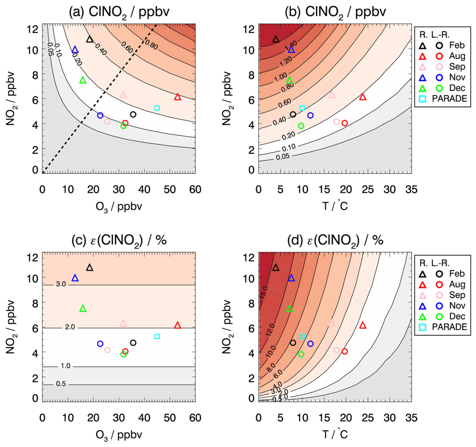
Figure 6Isopleth plot of modeled (a, b) ClNO2 mixing ratios that accumulate during the night and (c, d) the ClNO2 production efficiency depending on (a, c) the initial O3 and NO2 mixing ratios and (b, d) the temperature and initial NO2 mixing ratios. Values are taken 4 h after sunset, when maximum ClNO2 concentrations were observed. Symbols mark calculated ClNO2 mixing ratios for average values of NO2 and O3 mixing ratios measured in each period of the JULIAC campaign if the air masses originated either from long-range (L.-R.) or regional (R.) transportation. For comparison, values are also shown for measurements during the PARADE campaign in summer in Germany (Phillips et al., 2012). The dashed line (a) separates the regimes for which ClNO2 production is more sensitive to the change in O3 (a) and NO2 (d).
To further interpret the controlling factors of ClNO2 production, the dependence of ClNO2 production efficiency ε on NO2 and O3 is presented in Fig. 6c. The modeled ClNO2 production efficiency increases with increasing mixing ratios of NO2 but not with increasing O3 (Fig. 6c), as expected from Eq. (4), which shows that the ClNO2 production efficiency is a function of multiple parameters but not of the O3 mixing ratio. In general, the model reproduces the experimentally determined ClNO2 production efficiency (as shown in Fig. 5) within the uncertainty in the calculation (30 % to 40 %), which is mainly due to the assumptions concerning the history of air masses (Sect. 3.4). However, the relatively high ClNO2 production efficiency found in August and September in the regional air masses (Fig. 5) is significantly underestimated by the model. The discrepancy suggests that other processes facilitate the conversion from NO3 to ClNO2 in the regional air masses for summer-like conditions. Though the purpose of this model calculation is not to reproduce the observations, it is critical to address the related uncertainties/limitations due to the assumptions in the simplified model. The key parameters affecting the formation of ClNO2 concentrations are temperature, NO3 loss, and N2O5 loss. Their impact on the model results is discussed below.
Figure 6b shows the dependence of modeled ClNO2 on the temperature and NO2 concentrations investigated by the same model approach for which the O3 concentration is fixed to 30 ppbv (representing the typical O3 level of long-range transported air). In this case, the modeled ClNO2 concentrations reach maximum values at temperatures of 5 ∘C. For these winter-like conditions, the low temperature shifts the equilibrium between NO3 and N2O5 to the side of N2O5. In contrast, the conversion of NO2 to ClNO2 is suppressed at high temperatures (T > 15∘) under typical conditions in August and September. Temperature also plays an important role for the value of the ClNO2 production efficiency due to the shift in the equilibrium between NO3 and N2O5. The significantly higher ClNO2 production efficiency observed in February compared to the other seasons could be largely attributed to the low temperature at that time (Fig. 6d).
Sensitivity tests demonstrate that decreasing the rate of the chemical loss of NO3 to organic compounds (Fig. S11) only has a small impact, while the seasonal variation in chemical loss of NO3 peaks in summer-like conditions due to the intense biogenic emission. The higher production efficiency could be attributed to faster-than-assumed conversion from N2O5 to ClNO2, which can bring modeled and measured valued into agreement. This can be either achieved by increasing the value of the N2O5 uptake coefficient (Fig. S12) or the yield of ClNO2 in the process of the heterogeneous uptake of N2O5 on aerosol (Fig. S13).
As mentioned above, the NO3 reactivity is assumed to be 0.004 s−1 to match the observations, which is comparable to the NO3 reactivity observed at a mountainous site in southern Germany, with a campaign-averaged value of 0.01 s−1 for nighttime conditions (Liebmann et al., 2018). As shown in the sensitivity test, a higher NO3 reactivity leads to lower modeled ClNO2 concentrations. Therefore, the low NO3 reactivity in the model could be regarded as a lower limit given the similar biogenic-influenced environments.
In this model calculation, the aerosol surface area Sa is held constant instead of using the value measured inside the chamber, which was likely impacted by the sampling system, but cannot be corrected for ambient measurement (Sect. 2.3). Nevertheless, the measured Sa gives some confidence that the model is not using an unrealistic lower limit.
The aerosol chemical composition also plays a role in determining the production efficiency. The yield of ClNO2 from the N2O5 heterogenous reaction (φ(ClNO2)) can be expressed by assuming that the production of ClNO2 results from the competition between Cl− and H2O reacting with the H2ONO intermediate formed from the N2O5 uptake on aerosol (Bertram and Thornton, 2009; Mielke et al., 2013; McDuffie et al., 2018b).
The value of the ClNO2 yield is different in the periods of the campaign showing maximum values of 0.6 to 0.8 in February (Fig. S14). This is consistent with the relatively high ClNO2 production efficiency derived from the integrated production rate of NO3 (Eq. 7). However, the calculated ClNO2 yield decreases below 0.4 in August and September, which could be attributed to the higher aerosol liquid water content in these two periods compared to the value seen in other periods (Table S1). The calculated ClNO2 yield is also higher for the long-range transported air masses than those for the regional one (Fig. S14). The relatively high ClNO2 production efficiencies found in the regional air masses, which are in contrast with their relatively low calculated φ(ClNO2), suggest that other factors play an important role in determining the ClNO2 production, such as a larger-than-assumed uptake coefficient for N2O5 and/or aerosol surface area.
For comparison, the observation from another field campaign conducted in a similar rural environment in Germany is marked in the isopleth diagram (Fig. 6). The PARADE campaign took place in the Taunus Observatory of the University of Frankfurt, which is located 170 km southeast of the JULIAC measurement site (Phillips et al., 2012). The maximum observed ClNO2 mixing ratio was 0.8 ppbv when the measurement site was influenced by air masses from the UK/North Sea. This value is lower than the results of the model calculations using the median NO2 and O3 observed in that campaign, which is consistent with the general underprediction for summer-like conditions for the JULIAC campaign and suggests that the conversion from NO3 to ClNO2 is more efficient than the model predicts in summer. The position in the isopleth diagram suggests that ClNO2 formation was limited by the availability of NO2, similar to the summer period the JULIAC campaign, which is the same season as the PARADE campaign (August).
Concentrations of ClNO2 and other trace gases and the chemical composition of aerosols were measured during the Jülich Atmospheric Chemistry Project (JULIAC) campaign in 2019 that was performed at a rural site in Germany. Ambient air was sampled into the atmospheric simulation chamber SAPHIR from a height of 50 m, which was, most of the time, uncoupled from the surface layer during the night. Chamber characterization experiments demonstrated that no significant loss or production of ClNO2 occurred inside the chamber for experimental conditions of the JULIAC campaign.
In all periods, ClNO2 measurements showed a trend of increasing mixing ratios after sunset with maximum values were reached around midnight. This qualitative behavior is consistent with the chemical production of ClNO2 and insignificant losses during the night. Photolysis was the main loss process for ClNO2 on the following day. The maximum ClNO2 concentration in this campaign of 1.6 ppbv was observed in September during the early hours of the morning (03:00 UTC). The analysis of the origin of air masses by calculations of back trajectories shows that mixing ratios of ClNO2, NO2, and O3 were higher in regional air masses than in air masses that traveled a long distance.
A case study analyzing measurements at night from 21 to 22 August 2019 shows that the stratification of layers during the night can strongly impact observed trace gas concentrations, specifically when the sampling point of the inlet system was located within a height range that was characterized by poor vertical mixing of the air. During most times of the campaign, however, the sampling point was isolated from the surface layer during the night. In this case, losses of trace gases to the surface and reactions with fresh emissions on the ground, which would typically reduce ClNO2 production, were not important.
The ClNO2 production efficiency (i.e., the number of ClNO2 molecules formed per produced NO3 molecule) was higher for conditions in air masses from regional areas than from long-range transportation, mostly due to the higher NO2 mixing ratios. The minimum average value of the production efficiency calculated for the individual measurement periods in the JULIAC campaign was 3 % and was experienced in December for all air masses independent from their origin. This low value can be attributed to the low NO2 mixing ratios experienced in winter. For the air masses from long-range transportation, the mean ClNO2 production efficiencies were in the range of 3 % to 6 % in the period between August and November but were as high as 12 % in February, consistent with the seasonality of the observed ClNO2 concentrations. The highest mean ClNO2 production efficiency was found in February, when values reached 18 ± 9 % and NO2 concentrations were highest in the regional air masses. High ClNO2 production efficiency was also found in September when NO2 concentrations were low, suggesting that other factors including the available aerosol surface area (Sa), the variability in the N2O5 uptake coefficient, and the yield of ClNO2 in the heterogeneous reaction of N2O5 were favoring the production of ClNO2.
With the help of a simple box model of nighttime chemistry for the NO3-N2O5-ClNO2 system, the dependence of ClNO2 concentration on the availability of O3 and NO2 was investigated. The purpose of such a simplified model is to demonstrate the general feature of ClNO2 production versus chemical conditions but not to compare with observations. The model results suggest that ClNO2 production was more sensitive to the availability of NO2 than that of O3, especially for the air masses from long-range transportation. The seasonal variability in ClNO2 is less pronounced compared to the seasonal changes in NO2 and O3 concentrations because changes in the NO2 and O3 concentrations partly compensated for each other. The simple model cannot predict the seasonal changes in the observed ClNO2 mixing ratios. This indicates that processes other than the NO3 production rate significantly impacted the ClNO2 mixing ratios. Nevertheless, this simple model approach helps us to understand the general features of the dependence of ClNO2 concentrations on the availability of NO2 and O3 in the JULIAC campaign.
The data used in this study are available from the Jülich DATA platform (https://doi.org/10.26165/JUELICH-DATA/XG6YGZ; Tan et al., 2022).
The supplement related to this article is available online at: https://doi.org/10.5194/acp-22-13137-2022-supplement.
AH designed and organized the JULIAC campaign together with HF and FH. ZT and RS performed the measurements of ClNO2 and analyzed the data. ZT, RS, HF, and AH wrote the paper. All co-authors contributed with data and commented on and discussed the paper and contributed to the writing of this work.
At least one of the (co-)authors is a member of the editorial board of Atmospheric Chemistry and Physics. The peer-review process was guided by an independent editor, and the authors also have no other competing interests to declare.
Publisher's note: Copernicus Publications remains neutral with regard to jurisdictional claims in published maps and institutional affiliations.
The authors thank the scientific team of JULIAC campaign, for logistical support, and the Chemistry Workshop and Glassblower of the University of Leicester, for technical support.
This research has been supported by the H2020 European Research Council (SARLEP; grant no. 681529) and Eurochamp 2020 (grant no. 730997) and the Bundesministerium für Bildung und Forschung (ID-CLAR, grant no. 01DO17036; PRACTICE, grant no. 01LP1929A).
The article processing charges for this open-access publication were covered by the Forschungszentrum Jülich.
This paper was edited by Lisa Whalley and reviewed by two anonymous referees.
Atkinson, R., Baulch, D. L., Cox, R. A., Crowley, J. N., Hampson, R. F., Hynes, R. G., Jenkin, M. E., Rossi, M. J., and Troe, J.: Evaluated kinetic and photochemical data for atmospheric chemistry: Volume I - gas phase reactions of Ox, HOx, NOx and SOx species, Atmos. Chem. Phys., 4, 1461–1738, https://doi.org/10.5194/acp-4-1461-2004, 2004.
Bannan, T. J., Booth, A. M., Bacak, A., Muller, J. B. A., Leather, K. E., Le Breton, M., Jones, B., Young, D., Coe, H., Allan, J., Visser, S., Slowik, J. G., Furger, M., Prévôt, A. S. H., Lee, J., Dunmore, R. E., Hopkins, J. R., Hamilton, J. F., Lewis, A. C., Whalley, L. K., Sharp, T., Stone, D., Heard, D. E., Fleming, Z. L., Leigh, R., Shallcross, D. E., and Percival, C. J.: The first UK measurements of nitryl chloride using a chemical ionization mass spectrometer in central London in the summer of 2012, and an investigation of the role of Cl atom oxidation, J. Geophys. Res., 120, 5638–5657, https://doi.org/10.1002/2014JD022629, 2015.
Bertram, T. H. and Thornton, J. A.: Toward a general parameterization of N2O5 reactivity on aqueous particles: the competing effects of particle liquid water, nitrate and chloride, Atmos. Chem. Phys., 9, 8351–8363, https://doi.org/10.5194/acp-9-8351-2009, 2009.
Bohn, B., Rohrer, F., Brauers, T., and Wahner, A.: Actinometric measurements of NO2 photolysis frequencies in the atmosphere simulation chamber SAPHIR, Atmos. Chem. Phys., 5, 493–503, https://doi.org/10.5194/acp-5-493-2005, 2005.
Brown, S. S. and Stutz, J.: Nighttime radical observations and chemistry, Chem. Soc. Rev., 41, 6405–6447, https://doi.org/10.1039/c2cs35181a, 2012.
Brown, S. S., Dubé, W. P., Osthoff, H. D., Wolfe, D. E., Angevine, W. M., and Ravishankara, A. R.: High resolution vertical distributions of NO3 and N2O5 through the nocturnal boundary layer, Atmos. Chem. Phys., 7, 139–149, https://doi.org/10.5194/acp-7-139-2007, 2007.
Eger, P. G., Friedrich, N., Schuladen, J., Shenolikar, J., Fischer, H., Tadic, I., Harder, H., Martinez, M., Rohloff, R., Tauer, S., Drewnick, F., Fachinger, F., Brooks, J., Darbyshire, E., Sciare, J., Pikridas, M., Lelieveld, J., and Crowley, J. N.: Shipborne measurements of ClNO2 in the Mediterranean Sea and around the Arabian Peninsula during summer, Atmos. Chem. Phys., 19, 12121–12140, https://doi.org/10.5194/acp-19-12121-2019, 2019.
George, I. J. and Abbatt, J. P. D.: Heterogeneous oxidation of atmospheric aerosol particles by gas-phase radicals, Nat. Chem., 2, 713–722, https://doi.org/10.1038/nchem.806, 2010.
Jeong, D., Seco, R., Gu, D., Lee, Y., Nault, B. A., Knote, C. J., Mcgee, T., Sullivan, J. T., Jimenez, J. L., Campuzano-Jost, P., Blake, D. R., Sanchez, D., Guenther, A. B., Tanner, D., Huey, L. G., Long, R., Anderson, B. E., Hall, S. R., Ullmann, K., Shin, H., Herndon, S. C., Lee, Y., Kim, D., Ahn, J., and Kim, S.: Integration of airborne and ground observations of nitryl chloride in the Seoul metropolitan area and the implications on regional oxidation capacity during KORUS-AQ 2016, Atmos. Chem. Phys., 19, 12779–12795, https://doi.org/10.5194/acp-19-12779-2019, 2019.
Kercher, J. P., Riedel, T. P., and Thornton, J. A.: Chlorine activation by N2O5: simultaneous, in situ detection of ClNO2 and N2O5 by chemical ionization mass spectrometry, Atmos. Meas. Tech., 2, 193–204, https://doi.org/10.5194/amt-2-193-2009, 2009.
Le Breton, M., Hallquist, Å. M., Pathak, R. K., Simpson, D., Wang, Y., Johansson, J., Zheng, J., Yang, Y., Shang, D., Wang, H., Liu, Q., Chan, C., Wang, T., Bannan, T. J., Priestley, M., Percival, C. J., Shallcross, D. E., Lu, K., Guo, S., Hu, M., and Hallquist, M.: Chlorine oxidation of VOCs at a semi-rural site in Beijing: significant chlorine liberation from ClNO2 and subsequent gas- and particle-phase Cl–VOC production, Atmos. Chem. Phys., 18, 13013–13030, https://doi.org/10.5194/acp-18-13013-2018, 2018.
Liebmann, J. M., Muller, J. B. A., Kubistin, D., Claude, A., Holla, R., Plass-Dülmer, C., Lelieveld, J., and Crowley, J. N.: Direct measurements of NO3 reactivity in and above the boundary layer of a mountaintop site: identification of reactive trace gases and comparison with OH reactivity, Atmos. Chem. Phys., 18, 12045–12059, https://doi.org/10.5194/acp-18-12045-2018, 2018.
Liu, X., Qu, H., Huey, L. G., Wang, Y., Sjostedt, S., Zeng, L., Lu, K., Wu, Y., Hu, M., Shao, M., Zhu, T., and Zhang, Y.: High Levels of Daytime Molecular Chlorine and Nitryl Chloride at a Rural Site on the North China Plain, Environ. Sci. Technol., 51, 9588–9595, https://doi.org/10.1021/acs.est.7b03039, 2017.
Lou, S., Tan, Z., Gan, G., Chen, J., Wang, H., Gao, Y., Huang, D., Huang, C., Li, X., Song, R., Wang, H., Wang, M., Wang, Q., Wu, Y., and Huang, C.: Observation based study on atmospheric oxidation capacity in Shanghai during late-autumn: Contribution from nitryl chloride, Atmos. Environ., 271, 118902, https://doi.org/10.1016/j.atmosenv.2021.118902, 2022.
McDuffie, E. E., Fibiger, D. L., Dubé, W. P., Lopez-Hilfiker, F., Lee, B. H., Thornton, J. A., Shah, V., Jaeglé, L., Guo, H., Weber, R. J., Michael Reeves, J., Weinheimer, A. J., Schroder, J. C., Campuzano-Jost, P., Jimenez, J. L., Dibb, J. E., Veres, P., Ebben, C., Sparks, T. L., Wooldridge, P. J., Cohen, R. C., Hornbrook, R. S., Apel, E. C., Campos, T., Hall, S. R., Ullmann, K., and Brown, S. S.: Heterogeneous N2O5 Uptake During Winter: Aircraft Measurements During the 2015 WINTER Campaign and Critical Evaluation of Current Parameterizations, J. Geophys. Res., 123, 4345–4372, https://doi.org/10.1002/2018jd028336, 2018a.
McDuffie, E. E., Fibiger, D. L., Dubé, W. P., Lopez Hilfiker, F., Lee, B. H., Jaeglé, L., Guo, H., Weber, R. J., Reeves, J. M., Weinheimer, A. J., Schroder, J. C., Campuzano-Jost, P., Jimenez, J. L., Dibb, J. E., Veres, P., Ebben, C., Sparks, T. L., Wooldridge, P. J., Cohen, R. C., Campos, T., Hall, S. R., Ullmann, K., Roberts, J. M., Thornton, J. A., and Brown, S. S.: ClNO2 Yields From Aircraft Measurements During the 2015 WINTER Campaign and Critical Evaluation of the Current Parameterization, J. Geophys. Res., 123, 12994–13015, https://doi.org/10.1029/2018jd029358, 2018b.
McNamara, S. M., Kolesar, K. R., Wang, S., Kirpes, R. M., May, N. W., Gunsch, M. J., Cook, R. D., Fuentes, J. D., Hornbrook, R. S., Apel, E. C., China, S., Laskin, A., and Pratt, K. A.: Observation of Road Salt Aerosol Driving Inland Wintertime Atmospheric Chlorine Chemistry, ACS Cent. Sci., 6, 684–694, https://doi.org/10.1021/acscentsci.9b00994, 2020.
Mielke, L. H., Furgeson, A., and Osthoff, H. D.: Observation of ClNO2 in a mid-continental urban environment, Environ. Sci. Technol., 45, 8889–8896, https://doi.org/10.1021/es201955u, 2011.
Mielke, L. H., Stutz, J., Tsai, C., Hurlock, S. C., Roberts, J. M., Veres, P. R., Froyd, K. D., Hayes, P. L., Cubison, M. J., Jimenez, J. L., Washenfelder, R. A., Young, C. J., Gilman, J. B., de Gouw, J. A., Flynn, J. H., Grossberg, N., Lefer, B. L., Liu, J., Weber, R. J., and Osthoff, H. D.: Heterogeneous formation of nitryl chloride and its role as a nocturnal NOx reservoir species during CalNex-LA 2010, J. Geophys. Res., 118, 10638–10652, https://doi.org/10.1002/jgrd.50783, 2013.
Mielke, L. H., Furgeson, A., Odame-Ankrah, C. A., and Osthoff, H. D.: Ubiquity of ClNO2 in the urban boundary layer of Calgary, Alberta, Canada, Can. J. Chem., 94, 414–423, https://doi.org/10.1139/cjc-2015-0426, 2016.
Osthoff, H. D., Roberts, J. M., Ravishankara, A. R., Williams, E. J., Lerner, B. M., Sommariva, R., Bates, T. S., Coffman, D., Quinn, P. K., Dibb, J. E., Stark, H., Burkholder, J. B., Talukdar, R. K., Meagher, J., Fehsenfeld, F. C., and Brown, S. S.: High levels of nitryl chloride in the polluted subtropical marine boundary layer, Nat. Geosci., 1, 324–328, https://doi.org/10.1038/ngeo177, 2008.
Osthoff, H. D., Odame-Ankrah, C. A., Taha, Y. M., Tokarek, T. W., Schiller, C. L., Haga, D., Jones, K., and Vingarzan, R.: Low levels of nitryl chloride at ground level: nocturnal nitrogen oxides in the Lower Fraser Valley of British Columbia, Atmos. Chem. Phys., 18, 6293–6315, https://doi.org/10.5194/acp-18-6293-2018, 2018.
Phillips, G. J., Tang, M. J., Thieser, J., Brickwedde, B., Schuster, G., Bohn, B., Lelieveld, J., and Crowley, J. N.: Significant concentrations of nitryl chloride observed in rural continental Europe associated with the influence of sea salt chloride and anthropogenic emissions, Geophys. Res. Lett., 39, L10811, https://doi.org/10.1029/2012gl051912, 2012.
Priestley, M., le Breton, M., Bannan, T. J., Worrall, S. D., Bacak, A., Smedley, A. R. D., Reyes-Villegas, E., Mehra, A., Allan, J., Webb, A. R., Shallcross, D. E., Coe, H., and Percival, C. J.: Observations of organic and inorganic chlorinated compounds and their contribution to chlorine radical concentrations in an urban environment in northern Europe during the wintertime, Atmos. Chem. Phys., 18, 13481–13493, https://doi.org/10.5194/acp-18-13481-2018, 2018.
Riedel, T. P., Wagner, N. L., Dube, W. P., Middlebrook, A. M., Young, C. J., Ozturk, F., Bahreini, R., VandenBoer, T. C., Wolfe, D. E., Williams, E. J., Roberts, J. M., Brown, S. S., and Thornton, J. A.: Chlorine activation within urban or power plant plumes: Vertically resolved ClNO2 and Cl2 measurements from a tall tower in a polluted continental setting, J. Geophys. Res., 118, 8702–8715, https://doi.org/10.1002/jgrd.50637, 2013.
Roberts, J. M., Osthoff, H. D., Brown, S. S., Ravishankara, A. R., Coffman, D., Quinn, P., and Bates, T.: Laboratory studies of products of N2O5 uptake on Cl− containing substrates, Geophys. Res. Lett., 36, L20808, https://doi.org/10.1029/2009gl040448, 2009.
Rohrer, F., Bohn, B., Brauers, T., Brüning, D., Johnen, F.-J., Wahner, A., and Kleffmann, J.: Characterisation of the photolytic HONO-source in the atmosphere simulation chamber SAPHIR, Atmos. Chem. Phys., 5, 2189–2201, https://doi.org/10.5194/acp-5-2189-2005, 2005.
Simpson, W. R., Brown, S. S., Saiz-Lopez, A., Thornton, J. A., and von Glasow, R.: Tropospheric Halogen Chemistry: Sources, Cycling, and Impacts, Chem. Rev., 115, 4035–4062, https://doi.org/10.1021/cr5006638, 2015.
Sommariva, R., Hollis, L. D. J., Sherwen, T., Baker, A. R., Ball, S. M., Bandy, B. J., Bell, T. G., Chowdhury, M. N., Cordell, R. L., Evans, M. J., Lee, J. D., Reed, C., Reeves, C. E., Roberts, J. M., Yang, M., and Monks, P. S.: Seasonal and geographical variability of nitryl chloride and its precursors in Northern Europe, Atmos. Sci. Lett., 19, e844, https://doi.org/10.1002/asl.844, 2018.
Sommariva, R., Crilley, L. R., Ball, S. M., Cordell, R. L., Hollis, L. D. J., Bloss, W. J., and Monks, P. S.: Enhanced wintertime oxidation of VOCs via sustained radical sources in the urban atmosphere, Environ. Pollut., 274, 116563, https://doi.org/10.1016/j.envpol.2021.116563, 2021.
Stein, A. F., Draxler, R. R., Rolph, G. D., Stunder, B. J. B., Cohen, M. D., and Ngan, F.: NOAA's HYSPLIT Atmospheric Transport and Dispersion Modeling System, B. Am. Meteorol. Soc., 96, 2059–2077, https://doi.org/10.1175/bams-d-14-00110.1, 2015.
Tan, Z., Fuchs, H., Hofzumahaus, A., Bloss, W., Bohn, B., Cho, C., Hohaus, T., Holland, F., Lakshmisha, C., Liu, L., Monks, P., Novelli, A., Niether, D., Rohrer, F., Tillmann, R., Valkenburg, T., Vardhan, V., Kiendler-Scharr, A., Wahner, A., and Sommariva, R.: Data of ClNO2 for Campaign JULIAC 2019, Jülich DATA, V1 [data set], https://doi.org/10.26165/JUELICH-DATA/XG6YGZ, 2022.
Tham, Y. J., Wang, Z., Li, Q., Yun, H., Wang, W., Wang, X., Xue, L., Lu, K., Ma, N., Bohn, B., Li, X., Kecorius, S., Größ, J., Shao, M., Wiedensohler, A., Zhang, Y., and Wang, T.: Significant concentrations of nitryl chloride sustained in the morning: investigations of the causes and impacts on ozone production in a polluted region of northern China, Atmos. Chem. Phys., 16, 14959–14977, https://doi.org/10.5194/acp-16-14959-2016, 2016.
Thornton, J. A., Kercher, J. P., Riedel, T. P., Wagner, N. L., Cozic, J., Holloway, J. S., Dube, W. P., Wolfe, G. M., Quinn, P. K., Middlebrook, A. M., Alexander, B., and Brown, S. S.: A large atomic chlorine source inferred from mid-continental reactive nitrogen chemistry, Nature, 464, 271–274, https://doi.org/10.1038/nature08905, 2010.
Wagner, N. L., Dubé, W. P., Washenfelder, R. A., Young, C. J., Pollack, I. B., Ryerson, T. B., and Brown, S. S.: Diode laser-based cavity ring-down instrument for NO3, N2O5, NO, NO2 and O3 from aircraft, Atmos. Meas. Tech., 4, 1227–1240, https://doi.org/10.5194/amt-4-1227-2011, 2011.
Wagner, N. L., Riedel, T. P., Roberts, J. M., Thornton, J. A., Angevine, W. M., Williams, E. J., Lerner, B. M., Vlasenko, A., Li, S. M., Dube, W. P., Coffman, D. J., Bon, D. M., de Gouw, J. A., Kuster, W. C., Gilman, J. B., and Brown, S. S.: The sea breeze/land breeze circulation in Los Angeles and its influence on nitryl chloride production in this region, J. Geophys. Res., 117, D00V24, https://doi.org/10.1029/2012jd017810, 2012.
Wang, T., Tham, Y. J., Xue, L., Li, Q., Zha, Q., Wang, Z., Poon, S. C. N., Dubé, W. P., Blake, D. R., Louie, P. K. K., Luk, C. W. Y., Tsui, W., and Brown, S. S.: Observations of nitryl chloride and modeling its source and effect on ozone in the planetary boundary layer of southern China, J. Geophys. Res., 121, 2476–2489, https://doi.org/10.1002/2015JD024556, 2016.
Wang, X., Wang, H., Xue, L., Wang, T., Wang, L., Gu, R., Wang, W., Tham, Y. J., Wang, Z., Yang, L., Chen, J., and Wang, W.: Observations of N2O5 and ClNO2 at a polluted urban surface site in North China: High N2O5 uptake coefficients and low ClNO2 product yields, Atmos. Environ., 156, 125–134, https://doi.org/10.1016/j.atmosenv.2017.02.035, 2017.
Wang, Z., Wang, W., Tham, Y. J., Li, Q., Wang, H., Wen, L., Wang, X., and Wang, T.: Fast heterogeneous N2O5 uptake and ClNO2 production in power plant and industrial plumes observed in the nocturnal residual layer over the North China Plain, Atmos. Chem. Phys., 17, 12361–12378, https://doi.org/10.5194/acp-17-12361-2017, 2017.
Yan, C., Tham, Y. J., Zha, Q., Wang, X., Xue, L., Dai, J., Wang, Z., and Wang, T.: Fast heterogeneous loss of N2O5 leads to significant nighttime NOx removal and nitrate aerosol formation at a coastal background environment of southern China, Sci. Total Environ., 677, 637–647, https://doi.org/10.1016/j.scitotenv.2019.04.389, 2019.
Young, C. J., Washenfelder, R. A., Roberts, J. M., Mielke, L. H., Osthoff, H. D., Tsai, C., Pikelnaya, O., Stutz, J., Veres, P. R., Cochran, A. K., VandenBoer, T. C., Flynn, J., Grossberg, N., Haman, C. L., Lefer, B., Stark, H., Graus, M., de Gouw, J., Gilman, J. B., Kuster, W. C., and Brown, S. S.: Vertically resolved measurements of nighttime radical reservoirs in Los Angeles and their contribution to the urban radical budget, Environ. Sci. Technol., 46, 10965–10973, https://doi.org/10.1021/es302206a, 2012.
Yun, H., Wang, T., Wang, W., Tham, Y. J., Li, Q., Wang, Z., and Poon, S. C. N.: Nighttime NOx loss and ClNO2 formation in the residual layer of a polluted region: Insights from field measurements and an iterative box model, Sci. Total Environ., 622–623, 727–734, https://doi.org/10.1016/j.scitotenv.2017.11.352, 2018.
Zhou, W., Zhao, J., Ouyang, B., Mehra, A., Xu, W., Wang, Y., Bannan, T. J., Worrall, S. D., Priestley, M., Bacak, A., Chen, Q., Xie, C., Wang, Q., Wang, J., Du, W., Zhang, Y., Ge, X., Ye, P., Lee, J. D., Fu, P., Wang, Z., Worsnop, D., Jones, R., Percival, C. J., Coe, H., and Sun, Y.: Production of N2O5 and ClNO2 in summer in urban Beijing, China, Atmos. Chem. Phys., 18, 11581–11597, https://doi.org/10.5194/acp-18-11581-2018, 2018.