Correcting ozone biases in a global chemistry–climate model: implications for future ozone

Weaknesses in process representation in chemistry–climate models lead to biases in simulating surface ozone and to uncertainty in projections of future ozone change. We here develop a deep learning model to demonstrate the feasibility of ozone bias correction in a global chemistry–climate model. We apply this approach to identify the key factors causing ozone biases and to correct projections of future surface ozone. Temperature and the related geographic variables latitude and month show the strongest relationship with ozone biases. This indicates that ozone biases are sensitive to temperature and suggests weaknesses in representation of temperature-sensitive physical or chemical processes. Photolysis rates are also an important factor, highlighting the sensitivity of biases to simulated cloud cover and insolation. Atmospheric chemical species such as the hydroxyl radical, nitric acid and peroxyacyl nitrate show strong positive relationships with ozone biases on a regional scale. These relationships reveal the conditions under which ozone biases occur, although they reflect association rather than direct causation. We correct model projections of future ozone under different climate and emission scenarios following the shared socio-economic pathways. We find that changes in seasonal ozone mixing ratios from the present day to the future are generally smaller than those simulated without bias correction, especially in high-emission regions. This suggests that the ozone sensitivity to changing emissions and climate may be overestimated with chemistry–climate models. Given the uncertainty in simulating future ozone, we show that deep learning approaches can provide improved assessment of the impacts of climate and emission changes on future air quality, along with valuable information to guide future model development.

1 Introduction

Atmospheric chemical transport models have been developed over several decades with the principal purpose of simulating the composition of the atmosphere (Zhang, 2008), and chemistry schemes have been incorporated in chemistry–climate and earth system models to investigate the interactions between atmospheric composition and climate change (Flato, 2011). However, current chemistry–climate models are imperfect in simulating the concentration of atmospheric chemical species, even though they represent our latest understanding of the governing physical and chemical processes. Biases obtained through comparison with observations indicate that not all relevant processes can be adequately represented in models, and there are uncertainties associated with emissions, chemistry, transport, deposition, clouds and aerosols, in addition to structural errors associated with model resolution (Knutti and Sedláček, 2013; Archibald et al., 2020a). Representation of these processes may be biased due to poor understanding and simplified parameterisation, and the errors may propagate in complex earth system models.

While some models reproduce observed concentrations relatively well, this does not confirm that they represent the governing processes well, because biases arising from different processes may offset each other. Different models apply differing parameterisations of key processes, and even where these reflect current understanding, there may be large differences in model responses to changing conditions (Wild et al., 2020). This may lead to unreliable projections of changes in atmospheric composition under future emission and climate scenarios. However, it is difficult to identify the origin of biases in models, and this severely hinders model improvement and prevents a full understanding of the interactions between chemistry and climate through the earth system.

Tropospheric ozone (O₃) is an important greenhouse gas affecting climate and is a photochemical air pollutant at the earth's surface, damaging human health and ecosystems (Archibald et al., 2020a). Many studies show that the magnitude of the tropospheric O₃ burden and surface O₃ concentrations in remote areas can be simulated relatively well (Young et al., 2018; Griffiths et al., 2021). However, large differences still exist in simulated surface O₃ concentrations in high-emission areas (Turnock et al., 2020), and there are large uncertainties in temporal trends (Tarasick et al., 2019) that cannot be captured well by global chemistry–climate models (Parrish et al., 2021). In addition, structural biases in O₃ caused by coarse model resolution are hard to eliminate and typically lead to higher surface O₃ concentrations in polluted areas (Wild and Prather, 2006; Stock et al., 2014). Given the difficulty in resolving O₃ biases in a complex chemistry–climate model, the aim of this study is to correct simulations of present-day surface O₃ concentrations across the globe and to generate more reliable O₃ projections under future scenarios.

Machine learning provides a valuable approach to correct O₃ biases. Appropriate algorithms can be applied to identify the relationships between model responses and the driving variables based on extensive training. Deep learning approaches apply algorithms with more complex architectures and larger parameter spaces based on artificial neural networks (Goodfellow et al., 2016). In atmospheric science, machine learning has been successfully applied in some fields such as prediction of precipitation (Sønderby et al., 2020; Ravuri et al., 2021) and air pollution (Kleinert et al., 2021). Numerical approaches used in solving ordinary and partial differential equations in chemical and dynamic systems (Han et al., 2018; Keller and Evans, 2019), and in parameterising subgrid processes for clouds in climate models (Rasp et al., 2018), can also be replaced by machine learning to reduce computational costs. However, reliance on machine learning approaches to make predictions may lead to loss of interpretability of the results. We therefore choose an approach based on physical model variables that allows us to extract the importance of these variables and thus derive some physical insight into the performance of the chemistry–climate model.

In this study, we explore the application of deep learning to correct surface O₃ biases in a global chemistry–climate model, and we apply it for the first time to improve projections of changes in O₃ under future scenarios. We identify the dominant factors leading to O₃ biases with the aim of guiding future model development. We introduce the chemistry–climate model, present-day and future scenarios, and the deep learning model in Sect. 2. We demonstrate the performance of the deep learning model in Sect. 3. We show the importance of different variables to O₃ biases in Sect. 4, and how these vary by region in Sect. 5. We quantify surface O₃ biases in the present day and the future in Sect. 6, and show the importance for assessment of future O₃ changes in Sect. 7. We present our conclusions in Sect. 8.

2 Approach

2.1 Chemistry–climate model and experiments

We use version 1 of the United Kingdom Earth System Model, UKESM1 (Sellar et al., 2019), to simulate present-day (2004–2014) and future (2045–2055) surface O₃ mixing ratios under different emission and climate pathways. UKESM1 consists of a physical climate model, the Hadley Centre Global Environment Model version 3 (HadGEM3), with the Global Atmosphere 7.1 and Global Land 7.0 (GA7.1/GL7.0) configurations (Walters et al., 2019) for atmosphere-only simulations with prescribed sea surface temperatures, sea ice and greenhouse gas concentrations generated from the fully coupled UKESM1 (Meinshausen et al., 2017, 2020). Atmospheric composition is modelled with a state-of-the-art chemistry and aerosol module, the United Kingdom Chemistry and Aerosol model (UKCA; O'Connor et al., 2014), including a stratosphere–troposphere gas-phase chemistry scheme (StratTrop; Archibald et al., 2020b) and an aerosol scheme (GLOMAP-mode; Mulcahy et al., 2020). An extended chemistry scheme incorporating more reactive volatile organic compounds (VOCs) is used in this study to provide an improved representation of O₃ production environments (Liu et al., 2021). The model resolution is N96L85 in the atmosphere, with 1.875^∘ in longitude by 1.25^∘ in latitude, 85 terrain-following hybrid height layers and a model top at 85 km.

For present-day simulations, we use the Coupled-Model Intercomparison Project Phase 6 (CMIP6; Eyring et al., 2016) historical anthropogenic and biomass emissions from Hoesly et al. (2018) and Van Marle et al. (2017), respectively. Biogenic VOC emissions are calculated interactively in the Joint UK Land Environmental Simulator (JULES) land-surface scheme (Pacifico et al., 2011), which is coupled to UKCA. For future simulations, we use the shared socio-economic pathways (SSPs; O’Neill et al., 2014), which represent different pathways of emission and climate policies in the future accounting for social, economic and environmental development (Rao et al., 2017). We choose the SSP3-7.0 and SSP3-7.0-lowNTCF pathways to demonstrate the impacts of weak and strong air pollutant emission controls in the future, respectively. Both pathways lead to a warmer and more humid climate, but SSP3-7.0-lowNTCF has large reductions in anthropogenic emissions of near-term climate forcer (NTCF) species that include O₃ precursors and aerosols. Details of the present-day and future emissions under SSP3-7.0 and SSP3-7.0-lowNTCF can be found in Liu et al. (2022). Other emissions used here are the same as described in Turnock et al. (2020).

2.2 Deep artificial neural network

We here develop a deep learning model using a multilayer perceptron, as it is a fundamental approach to build artificial neural networks and easy to apply. More complex approaches such as convolutional or attention-based neural networks could be applied (LeCun et al., 2015; Vaswani et al., 2017), but multilayer perceptron neural networks are competitive and show good performance compared with other approaches (Tolstikhin et al., 2021). We hence choose a classical artificial neural network as an initial step to explore the possibility of O₃ bias correction; more complex approaches could be explored in future.

The multilayer perceptron neural network consists of an input layer, several hidden layers and an output layer, as shown in Fig. 1. In the hidden layers, we use three independent modules – a densely connected layer, a batch-normalisation layer (Ioffe and Szegedy, 2015) and a rectified linear unit (Relu; Glorot et al., 2011). Each layer has neurons that store data and associated weights. Neurons in densely connected layers connect to each neuron in the following layer. The batch-normalisation layers make the model training faster and more stable. The rectified linear unit is a non-linear activation function applied to the output of the previous layer. The deep learning model developed here is applied to correct surface O₃ mixing ratios solely simulated by UKESM1.

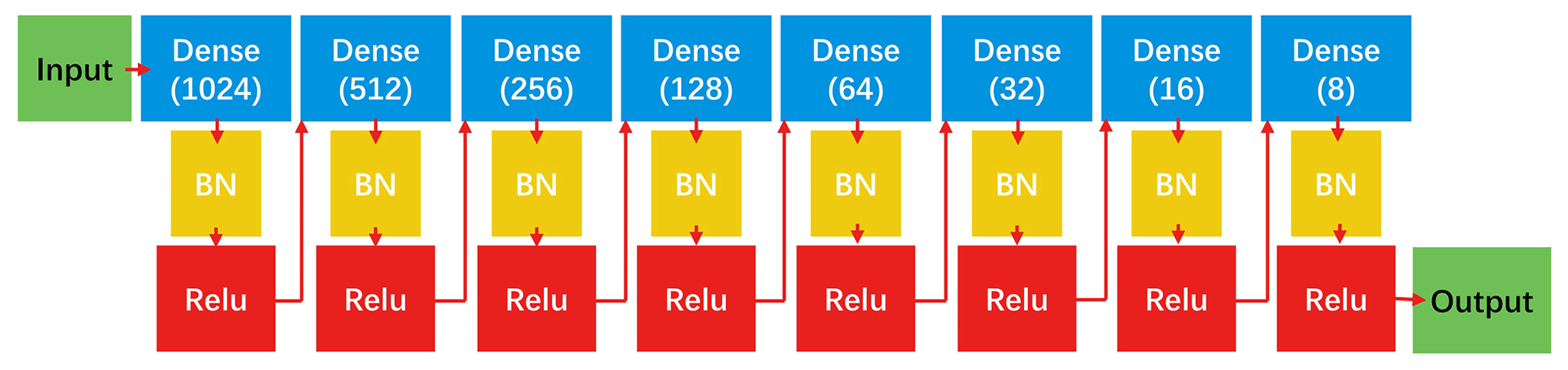
Figure 1 The structure of the deep artificial neural network built in this study. Each box represents one layer with neurons and weights to be passed to the next layer. In the densely connected layer (“Dense”), all neurons connect with neurons in the next layer, and the number of neurons is shown in brackets. In the batch-normalisation layer (“BN”), the data are normalised and passed to the next layer. The rectified linear unit (“Relu”) acts as a non-linear activation function. The arrows show the computation path from input to output.

2.3 Deep learning model input

Earth system models have numerous variables influencing surface O₃ mixing ratios, but including all variables as inputs for the deep learning model is impractical due to the heavy computational burden. It may also lead to overfitting, a common issue in machine learning associated with including more variables than can be justified by the limited volume of training data. Limiting the number of variables used as inputs also makes the results easier to interpret. In this exploratory study, we investigated more than 30 key input variables that represent the major large-scale influences on O₃ chemistry and transport, and settled on 20 variables that show the strongest relationships.

We consider major geographical and temporal variables including latitude, longitude, elevation, land cover and month. We define latitude from the Equator to the pole, and month from midwinter to midsummer in each hemisphere. Meteorological variables such as temperature, pressure, humidity, zonal and meridional wind are considered as they strongly influence O₃ chemical formation and transport. The sensitivity of O₃ to temperature is of particular interest, and has been shown to be a substantial source of uncertainty in current studies (Archibald et al., 2020c). Temperature and humidity have also been shown to influence O₃ variability on both regional and synoptic scales (Han et al., 2020; Shi et al., 2020). Two fundamental photolysis rates governing O₃ production and destruction, j(NO₂) and jO(¹D), are considered. Photolysis rates are strongly dependent on clouds, but there are large uncertainties in simulated cloud cover in current models (Wu et al., 2007; Voulgarakis et al., 2009; Hall et al., 2018). O₃ deposition rates and boundary layer height (BLH) are considered as they influence O₃ concentrations near the surface (O'Connor et al., 2014; Clifton et al., 2020). Concentrations of O₃ precursors such as nitric oxide (NO), VOCs (primary VOC species) and biogenic isoprene are considered, as these govern O₃ chemical production. The concentrations of hydroxyl radical (OH) and oxidative nitrogen species such as nitric acid (HNO₃) and peroxyacyl nitrates (PAN) are also considered because they reflect the general oxidation capacity of the atmosphere. HNO₃ and PAN are important nitrogen sinks that may transport nitrogen and affect O₃ formation over a wide area. Between them, the 20 variables selected represent some of the key drivers of uncertainty in simulating surface O₃, although we note that they are not independent of each other and that other factors may also be important under some conditions. We use O₃ mixing ratios from the lowest model layer of UKESM1, and normalise values of each input variable from zero to one.

2.4 Deep learning model application

Previous studies have shown that there are systematic seasonal biases in surface O₃ mixing ratios simulated with many chemistry–climate models (Young et al., 2018), including UKESM1 (Turnock et al., 2020). Ozone observations, such as those compiled for the Tropospheric Ozone Assessment Report (TOAR; Schultz et al., 2017), are typically used to evaluate model performance, but observation sites are sparsely distributed and there are few outside North America, Europe and parts of East Asia. In addition, many observations are representative of much smaller spatial scales than can be resolved by coarse-resolution models, and this presents an additional source of uncertainty.

We therefore also consider surface O₃ reanalysis data from the European Centre for Medium-Range Weather Forecasts (ECMWF) Atmospheric Composition Reanalysis 4 (EAC4) under the Copernicus Atmosphere Monitoring Service (CAMS; Inness et al., 2019). These data are at a similar spatial scale to UKESM1 output and provide global data coverage, which is valuable in training the deep learning model to ensure more robust results. We compare surface O₃ in UKESM1 with TOAR observations and CAMS reanalysis in Fig. 2. There are substantial biases in UKESM1, with surface O₃ underestimated compared to observations in wintertime and overestimated in summertime. In contrast, the CAMS reanalysis is in much better agreement with TOAR, with mean seasonal biases of about 3 ppb. Comparing UKESM1 and CAMS data over the globe, we find that mean surface O₃ mixing ratios over the 2004–2014 period simulated by UKESM1 are underestimated in the Northern Hemisphere in winter (December, January, February) and overestimated across most continental areas in summer (June, July, August), and this occurs over broad regions, not just where observations are available.

In the absence of a global observation-based ozone climatology, we apply the CAMS reanalysis product in our analysis. We note that recent studies have explored the fusion of observations and model output to generate surface O₃ products at a global scale (Chang et al., 2019; Betancourt et al., 2022), but these approaches only work well in regions where measurement sites are available. The CAMS reanalysis provides surface concentrations at a scale comparable with our model, and thus avoids uncertainties associated with the spatial representativeness of observations when using measured concentrations. While biases in the reanalysis will influence our results, the CAMS data provide a good foundation with which to demonstrate the feasibility of O₃ bias correction.

Figure 2 Comparison of seasonal mean (December–January–February (DJF) and June–July–August (JJA)) and annual mean surface O₃ mixing ratios between (a–c) UKESM1 and TOAR, (d–f) CAMS and TOAR, and (g–i) UKEMS1 and TOAR, all averaged over 2004–2014. Global area-weighted average surface mean mixing ratios (ppb) are shown in the top right of each panel.

2.5 Model training

The deep learning model is trained to reproduce the O₃ bias in each UKESM1 grid cell based on the corresponding values of the input variables. We train the deep learning model using the biases of monthly mean surface O₃ mixing ratios from each model grid cell over 2004–2014 (192 longitudes × 144 latitudes × 12 months × 11 years = 3.6 million data samples). We randomly split the data into training data (80 %), validation data (10 %) and testing data (10 %). Training data are only used to train the model. The validation data provide an evaluation of model performance for each iteration of training and the testing data are used to provide an independent evaluation once model training is complete.

The performance of the deep learning model is dependent on the volume of data and the settings used, and we experiment with a range of different settings to keep a balance between training speed and accuracy. We choose an Adam optimiser for the training algorithm (Kingma and Ba, 2014) and use mean absolute error for the loss function in this study. We use 0.01 as the model learning rate and 1024 grid boxes as the training batch size for stochastic gradient descent. Among these settings, we find that the batch size is the most important factor influencing model performance. 1024 randomly sampled data points account for about 4 % of the data from all grid cells in 1 month in each training iteration, and we find that this is adequate to represent different situations of O₃ biases and is found to be sufficient to train the model well.

3 Deep learning model performance

We determine the deep learning model performance in predicting surface O₃ biases using the testing data to give an independent evaluation (Fig. 3). The model reproduces the surface O₃ biases well, with a high correlation coefficient of 0.99 and a mean bias error of 0.1 ppb and root-mean-square error of 1.9 ppb. The frequency distribution of surface O₃ biases predicted by the deep learning model is very similar to that calculated using the O₃ reanalysis data. The tails of the distribution also match well, indicating that large biases can be reproduced well. The evaluation demonstrates that the input variables selected are sufficient to predict surface O₃ biases well.

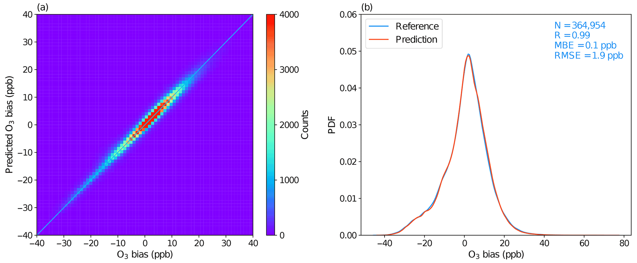
Figure 3 Evaluation of the deep learning model in simulating monthly mean surface O₃ biases at each UKESM1 grid point based on testing data. (a) O₃ biases (UKESM1 minus CAMS) and biases predicted by the deep learning model. (b) Probability density function of O₃ biases (labelled here as Reference) and predicted O₃ biases. Statistics are shown in the top right corner.

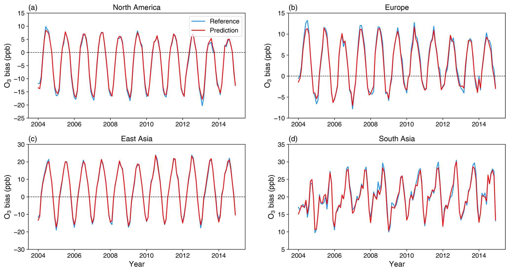
Figure 4 Monthly mean surface O₃ biases (UKESM1 minus CAMS; Reference) and O₃ biases predicted by the deep learning model in (a) North America, (b) Europe, (c) East Asia and (d) South Asia from January 2004 to December 2014.

To investigate the spatial and temporal behaviour of the model performance, we focus on surface O₃ biases in the present-day high-emission regions of North America, Europe, East Asia and South Asia (Fig. 4). North America, Europe and East Asia all show systematic negative surface O₃ biases in winter and positive biases in summer (Fig. 4a–c). South Asia shows different behaviour, with consistent positive biases for all months (Fig. 4d). O₃ biases in South Asia show more fluctuations over the annual cycle than those in other regions, but these fluctuations are also captured well by the deep learning model. We note that the magnitudes of O₃ biases are simulated well, and that the differences from year to year are also captured accurately. These four regions demonstrate that the deep learning model is able to predict regional differences and their respective magnitudes well.

4 Feature importance

While all input variables contribute to the prediction of O₃ biases, their relative contributions are different and can be estimated to determine which ones are dominant. An advanced unified framework for interpreting predictions of machine learning models, Shapley additive explanations (SHAP; Lundberg and Lee, 2017), is used to calculate the contribution of different variables to the predicted biases. The feature importance is represented by the SHAP value, which provides a quantitative measure of the variable contribution, as shown in Fig. 5. We calculate SHAP values for each variable using 100 sets of 100 data points randomly selected from the full distribution, and show their mean values and one standard deviation. The colours indicate the underlying relationships between the O₃ biases and the selected variables based on the correlation between the calculated SHAP values and variable values. Red represents a strong positive relationship (r>0.7), blue represents a strong negative relationship ($r<-\mathrm{0}$.7) and grey shows weaker relationships.

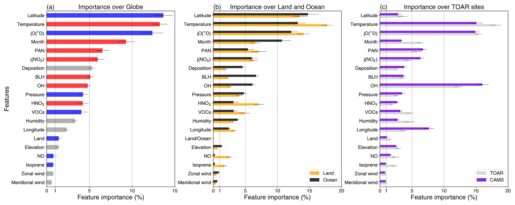
Figure 5 Importance of different variables to surface O₃ biases calculated by the Shapley additive explanations framework (SHAP) for the deep learning model. (a) Feature importance over the globe derived from CAMS reanalysis data. Strong positive (r>0.7) and negative ($r<-\mathrm{0}$.7) relationships between O₃ biases and variable values are shown in red and blue, respectively, while weaker relationships are shown in grey. (b) Feature importance over land and ocean regions derived from CAMS reanalysis data. (c) Comparison of feature importance inferred from CAMS and TOAR separately at the TOAR measurement locations only. Error bars show one standard deviation of feature importance in % for each variable.

We find that latitude and month are important to O₃ biases and show negative and positive relationships with surface O₃ biases, respectively. This reflects more positive biases in tropical regions than at the poles, and more positive biases in summer than winter. Temperature also shows a strong positive relationship, and this may partly reinforce the influence of latitude and month. Photolysis rates are also important for O₃ biases, with jO(¹D) associated with O₃ destruction and j(NO₂) with O₃ production. The concentrations of PAN, OH and HNO₃ all show positive relationships with O₃ biases. This may indicate that there are large uncertainties in O₃ production in high-oxidation and high-NO_x environments. However, we find that VOCs and short-lived NO concentrations are less important to O₃ biases. This highlights the systematic regional and global-scale nature of the O₃ biases in UKESM1, and indicates that the biases are not strongly associated with precursor abundance on a regional level. Similarly, isoprene concentrations show little contribution to O₃ biases. We note that while O₃ deposition rates and BLH are both important to O₃ biases, this may partly reflect their similar seasonality. Previous studies investigating model O₃ biases have found a broadly similar importance for some variables, e.g. for time of year and precursors such as PAN, but the different focus of these studies makes direct comparison of the results difficult (Ivatt and Evans, 2020; Keller et al., 2021).

To highlight the sensitivity of our results to the physical and chemical environment, we show the feature importance over land and ocean regions separately in Fig. 5b. Ozone precursors such as NO, isoprene and VOCs are much more important over land, along with some physical variables such as temperature. In contrast, O₃ biases over the ocean are more sensitive to OH, deposition and boundary layer mixing. These differences reflect the differing importance of O₃ formation and removal processes in the different regions, although we find that the dominant variables such as temperature and photolysis rates remain important for both regions.

We also calculate feature importance at the TOAR measurement locations only and compare use of surface O₃ from TOAR and CAMS separately, to explore the sensitivity of our results to the choice of reference data. We find that the feature importance at these locations differs markedly from that over the globe for some variables, particularly for OH and for geographical variables such as latitude and longitude. These differences reflect the limited spatial coverage of measurement sites and the narrower range of chemical environments sampled. However, the feature importance is very similar whether using TOAR measurements or CAMS reanalysis O₃ at these same locations, demonstrating that these datasets provide very similar information, and this lends confidence in our choice of CAMS reanalysis data for our analysis.

The relationships between variables with the highest feature importance and the O₃ biases are generally directly interpretable, demonstrating that the deep learning model may be capturing the internal relationships between inputs and outputs in a physically realistic way. This provides some insight into the sources of O₃ biases in UKESM1. We emphasise that the high importance of a variable does not indicate that the variable itself is not simulated well by the chemistry–climate model, or that it is the direct cause of the bias. Since temperature is generally represented well in UKESM1 (Sellar et al., 2019), the importance of temperature thus indicates that O₃ biases may be caused by the representation of physical and chemical processes that are sensitive to temperature change, such as chemical reaction rates (Coates et al., 2016; Newsome and Evans, 2017), or to other processes for which temperature is a proxy, and this explains the seasonality of the reversal in O₃ biases from winter to summer in the Northern Hemisphere.

Specifically for UKESM1, Archibald et al. (2020c) found that the O₃ responses to the same temperature changes in two chemical mechanisms (including StratTrop of UKESM1) are distinct, suggesting that temperature may be a main source of biases. In addition, more comprehensive chemistry schemes based on StratTrop further enlarge the O₃ biases in summer, as reported by Archer-Nicholls et al. (2021) and Liu et al. (2022), indicating that the chemistry scheme itself may not be the main cause of biases but the external variables driving the scheme, e.g. temperature and photolysis rates may be more important. We note that the relationships derived between the variables and O₃ biases reflect association, not causation, and that specific processes cannot be identified directly as the sources of biases. However, the association revealed provides some hints for the underlying processes associated with relevant variables.

5 Spatial O₃ bias sensitivity

The sensitivity of surface O₃ biases to specific variables differs across regions, and we show the spatial sensitivity to variables with high feature importance and strong correlation to O₃ biases in Fig. 6. Since each variable is considered independent in the deep learning model, we use the change in annual mean O₃ bias caused by changes in each variable in each UKESM1 grid cell independently to represent the spatial sensitivity. We perform an experiment for each variable where we increase the value of that variable by a small amount (0.5 standard deviations of its temporal variability over 2004–2014) and calculate the corresponding change in surface O₃.

Figure 6 Sensitivity of annual mean surface O₃ bias to increases in (a) temperature, (b) jO(¹D), (c) j(NO₂), (d) OH, (e) PAN and (f) BLH. Variable values are increased by 0.5 standard deviations of their temporal variability for each UKESM1 grid cell independently.

Surface O₃ biases are most sensitive to temperature, particularly in continental areas in the Northern Hemisphere where higher temperatures are associated with higher O₃ (Fig. 6a). There is a strong relationship with photolysis rates across a large area, particularly in continental areas at mid and high latitudes (Fig. 6b, c), and there is a larger influence from jO(¹D) than from j(NO₂). The chemical environment is important for O₃ biases on a regional scale. OH concentrations show a strong association with O₃ biases in North America, Europe and East Asia, indicating that high biases in these high-emission regions may be associated with high atmospheric oxidation capacity (Fig. 6d). There is also a strong sensitivity to the concentrations of PAN in South Africa, South Asia and South East Asia (Fig. 6e). This may indicate uncertainty in the NO_x emission inventory in these regions or the large impacts of nitrogen reservoirs on O₃ production. Given the long lifetime of PAN, it is also associated with O₃ biases in remote areas such as the Arctic, indicating that the transport of air pollutants may be important to surface O₃ in these areas. BLH is associated with O₃ biases in tropical oceanic areas (Fig. 6f), and this may reveal the importance of greater O₃ mixing and downward transport when the boundary layer is relatively deep.

The spatial sensitivity of surface O₃ biases to different variables is helpful for guiding future improvement of the UKESM1 model. There are substantial changes in annual mean surface O₃ biases associated with adjusting variables' values. Increasing temperature, jO(¹D), j(NO₂), OH and PAN concentrations by 0.5 standard deviations changes annual mean surface O₃ biases from 4.0 to 4.8 ppb (20 %), 3.0 ppb (−25 %), 4.3 ppb (8 %), 4.5 ppb (13 %) and 4.7 ppb (18 %), respectively. However, we note that UKESM1 generally reproduces temperature and photolysis rates well compared with observations (Telford et al., 2013; Sellar et al., 2019), although there are large differences in simulated concentrations of OH and PAN (O'Connor et al., 2014; Nicely et al., 2020). Our results suggest that chemical processes associated with temperature and oxidation capacity, and cloud and aerosols influencing photolysis rates, may be important sources of O₃ biases in UKESM1, and that improved representation of these processes may reduce current biases in surface O₃.

6 Assessing biases in modelled future surface O₃

We can apply the relationships between variables and surface O₃ biases derived from present-day simulations to assess the biases in future O₃ projections with UKESM1 and to correct our estimates of future O₃ concentrations. We demonstrate how surface O₃ biases change for two future emission and climate scenarios, SSP3-7.0 and SSP3-7.0-lowNTCF. These pathways are associated with a warmer and more humid climate than in the present day. While increased temperature might be expected to increase surface O₃ biases, we find that annual mean O₃ biases decrease from 4.0 to 3.6 ppb (11 %) under SSP3-7.0 and to 1.3 ppb (67 %) under SSP3-7.0-lowNTCF. This is principally due to changes in the chemical environment reflected by decreases in the concentrations of OH (−15 % and −13 %) and PAN (−30 % and −38 %) under SSP3-7.0 and SSP3-7.0-lowNTCF, respectively. In continental areas where surface O₃ concentrations are overestimated, the UKESM1 model performance is likely to improve under these less polluted future conditions. Since SSP3-7.0-lowNTCF represents a more stringent emission-control pathway than SSP3-7.0, there are larger decreases in O₃ biases under this scenario.

We investigate the spatial distribution of annual mean changes in surface O₃ biases in future scenarios. We find that O₃ biases decrease in most oceanic areas under both future scenarios, see Fig. 7. However, O₃ biases increase in some continental areas, especially in the Middle East, South Asia and East Asia, under SSP3-7.0. This is due to less stringent emission controls in these regions and hence higher concentrations of O₃ precursors and their oxidation products under SSP3-7.0 (Turnock et al., 2020). Under SSP3-7.0-lowNTCF, there are widespread decreases in O₃ biases except over East Asia, where anthropogenic VOC emissions increase substantially and there is a corresponding increase in PAN concentrations and an increase in O₃ biases. In high-emission regions, the performance of UKESM1 in future O₃ simulations largely depends on changes in O₃ precursor emissions, given that changes in temperature and photolysis rates are small under future scenarios. The performance of UKESM1 in high-emission regions is expected to improve under scenarios with clean air quality policies, but is likely to become worse under scenarios with increasing future pollutant emissions.

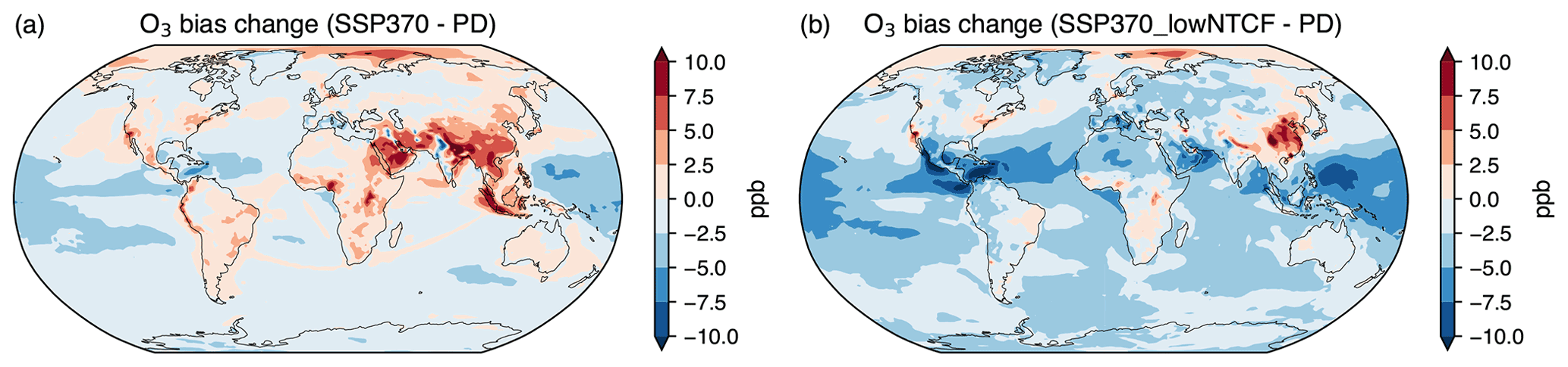
Figure 7 Annual mean change in surface O₃ biases (ppb) between the present day (PD) and 2045–2055 under (a) SSP3-7.0 and (b) SSP3-7.0-lowNTCF pathways.

7 Bias correction in future O₃ projections

We can provide more reliable projections of future O₃ by subtracting the calculated surface O₃ biases from surface O₃ mixing ratios simulated with UKESM1 under future scenarios (Fig. 8). The simulated surface O₃ mixing ratios vary in the different scenarios due to different emissions and climate (Fig. 8a–c), but the spatial distributions are generally similar, with the highest O₃ levels in the Middle East and South Asia. The spatial patterns of surface O₃ biases are also similar under the different scenarios, with biases highest in the tropics (Fig. 8d–f). High O₃ mixing ratios in the Middle East and South Asia are reduced greatly after O₃ bias correction (Fig. 8g–h). There are also large decreases in surface O₃ mixing ratios in high-emission regions, e.g. North America and East Asia, and continental outflow regions, e.g. the North Atlantic. The corrected global annual mean surface O₃ mixing ratios are lower than those simulated under all scenarios, and are highest under SSP3-7.0 and lowest under SSP3-7.0-lowNTCF, which is consistent with the uncorrected UKESM1 results.

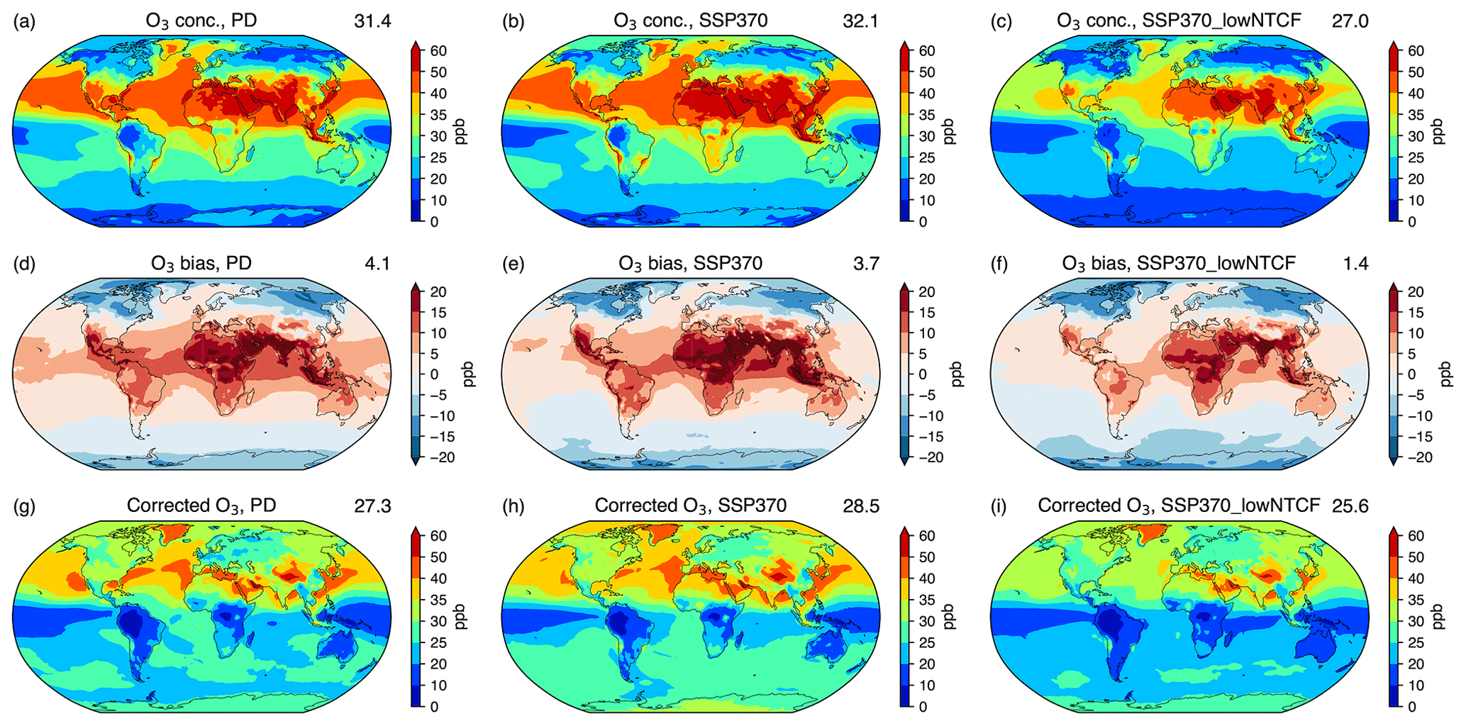
Figure 8 Annual mean surface O₃ mixing ratios (ppb) from UKESM1 simulations for (a) the present day (PD), (b) SSP3-7.0 and (c) SSP3-7.0-lowNTCF. The corresponding surface O₃ biases predicted with the deep learning model are shown in panels (d)–(f) and corrected surface O₃ mixing ratios are shown in panels (g)–(i). Annual global mean mixing ratios are shown in the top right of each panel.

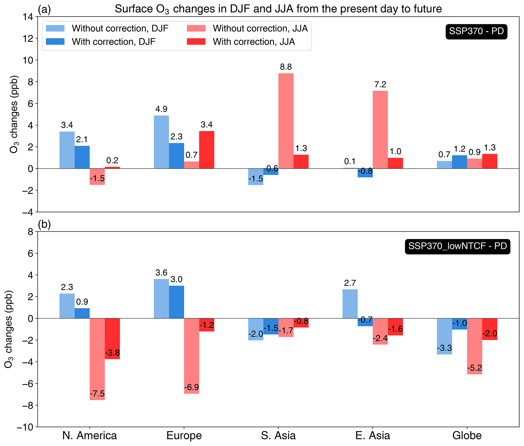
Figure 9 Changes in seasonal mean surface O₃ mixing ratios (ppb) with and without corrections in DJF (blue bars) and JJA (red bars) from the present day (PD) to (a) SSP3-7.0 and (b) SSP3-7.0-lowNTCF in North America, Europe, South Asia, East Asia and the globe.

We show the changes in seasonal mean surface O₃ mixing ratios in North America, Europe, South Asia, East Asia and the globe from the present day to the future in Fig. 9, comparing the original assessments using UKESM1 with the bias-corrected values. Under SSP3-7.0, the corrected changes in global mean surface O₃ are slightly larger than the uncorrected UKESM1 results. However, in high-emission regions, the corrected changes are generally smaller than those originally simulated under both SSP3-7.0 and SSP3-7.0-lowNTCF. In summer, corrected surface O₃ mixing ratios increase in all regions considered here under SSP3-7.0, and decrease under SSP3-7.0-lowNTCF. Corrected O₃ increases in South and East Asia under SSP3-7.0 are 6–8 ppb smaller than those simulated, and this indicates that O₃ air quality degradation due to future emission growth and climate change may not be as severe as the uncorrected UKESM1 simulations suggest. Similarly, under SSP3-7.0-lowNTCF, corrected O₃ decreases are smaller in all regions, and this indicates that the impacts of emission controls on O₃ mitigation may be smaller than those expected. This can be confirmed by the smaller global mean O₃ decreases under SSP3-7.0-lowNTCF in the bias-corrected assessment (< 2 ppb) than in the original UKESM1 simulation (> 3 ppb). In winter, the corrected changes in surface O₃ mixing ratios are smaller than those simulated with UKESM1, regardless of whether these changes are positive or negative.

These results highlight that the influence of changing emissions and climate on O₃ may not be as large as those simulated with UKESM1 and, thus, projections of future surface O₃ changes may be overestimated. UKESM1 shows a strong seasonality of surface O₃, likely due to strong O₃ sensitivity to temperature and the chemical environment, and this leads to large changes in future O₃. UKESM1 typically overestimates future surface O₃ changes, and other chemistry–climate models are likely to display similar behaviour. Therefore, the impacts of changes in emissions and climate on future O₃ should be re-assessed in light of the underlying surface O₃ biases. We demonstrate the successful application of a deep learning model to address this issue, and it would be valuable to take a similar approach with the output of other chemistry–climate models to provide a more reliable assessment of future surface O₃ changes.

8 Conclusions

There are large uncertainties in the simulation of surface O₃ in current chemistry–climate models, but it is difficult to identify the causes of biases and improve representation of the key processes. In this study, we have demonstrated the feasibility of correcting surface O₃ biases for a chemistry–climate model, UKESM1, using a machine learning technique. A deep artificial neural network is built with input variables important for O₃ chemistry and dynamics. The deep learning model shows good performance in predicting surface O₃ biases, with a high correlation coefficient of 0.99 and small mean bias errors of 0.1 ppb. Application of the deep learning model to the results from the process-based UKESM1 model shows promise for predicting future O₃ concentrations under different climate and emission trajectories with greater confidence.

This study has also explored the key factors governing O₃ biases, which provides valuable insight for model improvement. We find that temperature is an important factor governing O₃ biases, especially for continental areas in the Northern Hemisphere, indicating that physical and chemical processes influenced by temperature may be not represented well. Photolysis rates also contribute to O₃ biases across the globe, indicating that simulated clouds and aerosols may be an important source of O₃ biases. Chemical species such as PAN and OH are closely associated with O₃ biases on a regional scale, suggesting that weaknesses in representation of key chemical processes remains a substantial issue.

We have applied a deep learning model to generate a correction to the projections of surface O₃ mixing ratios for the present day and under future SSP3-7.0 and SSP3-7.0-lowNTCF pathways. We find that global annual mean O₃ biases (4.0 ppb) decrease by 0.4 ppb (11 %) and 2.7 ppb (67 %) under these future scenarios, respectively. However, O₃ biases in high-emission areas may increase due to increased O₃ precursors. We use this approach to demonstrate that seasonal changes in surface O₃ mixing ratios from the present day to the future may be overestimated by as much as 6 ppb with UKESM1, especially in high-emission areas, and this highlights a strong O₃ sensitivity to changes in future emissions and climate in the model. A similar overestimation of future O₃ changes is likely in other chemistry–climate models, and the influence of emission controls on surface O₃ mixing ratios may thus be smaller than suggested by current model simulations. This suggests that emission-control policies may be less effective in improving regional air quality than global model simulations indicate.

The deep learning model employed here is a valuable tool for obtaining more reliable predictions of the magnitude and spatial distribution of surface O₃ mixing ratios. We acknowledge that the choice of input variables and the machine learning approach applied are both likely to influence the sensitivity of O₃ biases derived from the deep learning model, and the relationships between O₃ biases and input variables are not always readily interpretable, which is common in machine learning. However, we demonstrate that the relationships between the variables with the highest feature importance and surface O₃ biases are intuitive, e.g. with temperature and photolysis rates, and this provides useful insight for further model improvement. While we are not able to identify the specific processes leading to biases using this approach, it allows us to target processes that are most sensitive to these variables. It would be valuable to develop explainable machine learning algorithms to use for bias correction. We also note that there are weaknesses in the representation of O₃ in the reanalysis data, which are likely to affect the magnitude of the biases we have derived. However, we have successfully demonstrated the feasibility of bias correction using these data, and will explore the challenges of data sparsity and spatial representativeness associated with use of surface measurements directly in future work. This approach should also be directly applicable for models with smaller initial biases, and in this case it would be particularly valuable to consider daily or hourly mean O₃ to explore representation of synoptic and diurnal variations in O₃. However, development of robust and reliable surface O₃ climatology based on observations would be particularly useful to improve the assessment of model biases. The approach applied here provides a valuable opportunity to examine the uncertainties in a chemistry–climate model, and helps improve assessment of the impacts of changing emissions and climate on future air quality.