How do gravity waves triggered by a typhoon propagate from the troposphere to the upper atmosphere?

Gravity waves (GWs) strongly affect atmospheric dynamics and photochemistry and the coupling between the troposphere, stratosphere, mesosphere, and thermosphere. In addition, GWs generated by strong disturbances in the troposphere (e.g. thunderstorms and typhoons) can affect the atmosphere of Earth from the troposphere to the thermosphere. However, the fundamental process of GW propagation from the troposphere to the thermosphere is poorly understood because it is challenging to constrain this process using observations. Moreover, GWs tend to dissipate rapidly in the thermosphere because the molecular diffusion increases exponentially with height. In this study, a double-layer airglow network was used to capture concentric GWs (CGWs) over China that were excited by Typhoon Chaba (2016). We used ERA5 reanalysis data and Multi-functional Transport Satellite-1R observations to quantitatively describe the propagation processes of typhoon-generated CGWs from the troposphere, through the stratosphere and mesosphere, to the thermosphere. We found that the CGWs in the mesopause region were generated directly by the typhoon in the troposphere. However, the backward-ray-tracing analysis suggested that CGWs in the thermosphere originated from the secondary waves generated by the dissipation of the CGW and/or nonlinear processes in the mesopause region.

1 Introduction

Gravity waves (GWs) can transfer momentum and energy from the lower to the upper atmosphere, thereby affecting global circulation and the thermal and compositional structures in the middle and upper atmospheres (Holton, 1983; Fritts and Alexander, 2003). Studies of dynamical, photochemical, and electrodynamics processes have indicated that GWs are fundamental for the coupling process between the troposphere, stratosphere, mesosphere, and thermosphere (Liu and Vadas, 2013; Smith et al., 2013; Vadas and Liu, 2013; Xu et al., 2015; Vadas and Becker, 2019).

Concentric GWs (CGWs) are a unique type of GW and considered to be mainly generated by convective activity in the troposphere. CGWs can also be generated by GW-breaking (Vadas and Becker, 2019; Lund et al., 2020; Kogure et al., 2020) volcanoes (Duncombe, 2022), nuclear explosions (Pfeffer and Zarichny, 1962; Pierce al., 1971), and rockets (Liu et al., 2018). CGWs in the stratosphere and mesosphere generated by thunderstorms have been widely reported, since their sources are ubiquitous (Taylor and Hapgood, 1988; Sentman et al., 2003; Suzuki et al., 2007; Yue et al., 2009; Vadas et al., 2012; Xu et al., 2015; Heale et al., 2019; Smith et al., 2020). In addition, Liu et al. (2014) utilized the Whole Atmosphere Community Climate Model to study the global CGWs. In previous studies, CGWs induced by typhoons were detected using ground-based optical remote sensing (Suzuki et al., 2013), while those induced by hurricanes and tropical cyclones were detected using the Suomi National Polar-orbiting Partnership satellite (Yue et al., 2014; Xu et al., 2019) in the mesopause region.

Notably, GWs tend to dissipate rapidly in the upper atmosphere due to molecular viscosity and thermal diffusion (Vadas, 2007). Thermosphere GWs that are not dissipated can originate directly from the troposphere (Vadas, 2007; Azeem et al., 2015) or from secondary GWs, which are generated from the breaking of primary GWs in the mesosphere or thermosphere region (Vadas et al., 2003; Vadas and Crowley, 2010; Vadas and Azeem, 2021). Furthermore, Vadas and Becker (2019) for the first time presented global simulations of tertiary CGWs from the dissipation of secondary CGWs in the thermosphere. Moreover, wave–wave interaction, wave–mean flow interaction (Franke and Robinson, 1999; Vadas and Fritts, 2001), self-acceleration, and nonlinear breaking are other potential secondary wave generation mechanisms (Lund and Fritts, 2012; Fritts et al., 2015; Dong et al., 2020; Fritts et al., 2020; Zhou et al., 2002; Heale et al., 2020). At the same time, tunnelling has been deemed a mechanism that can couple waves from tropospheric sources to the thermosphere (Walterscheid and Hecht, 2003; Gavrilov and Kshevetskii; 2018, Heale et al., 2021). However, the lack of observations of the entire atmosphere limits our understanding of the fundamental process of how GWs propagate from the lower to the upper atmosphere step by step on the aspect of observations.

This paper presents a case study examining CGWs excited by Typhoon Chaba (2016). To this end, we utilized Multi-functional Transport Satellite-1R (MTSAT-1R) observations, multi-layer European Centre for Medium-Range Weather Forecasts (ECMWF) ERA5 reanalysis data (Hoffmann et al., 2019; Hersbach et al., 2020), and high-spatiotemporal-resolution double-layer airglow network (DLAN) (Xu et al., 2021) observations. The CGW observations from the troposphere to the stratosphere and then to the mesosphere were taken from MTSAT-1R, ERA5, and the DLAN. However, given the observational limitations between the mesosphere and thermosphere, the two layers are connected by ray-tracing theory. The objectives of this study were to (a) investigate multi-layer CGW features produced by Typhoon Chaba (2016) from near the ground to a height of 250 km, (b) examine the entire propagation process of the CGWs excited by the typhoon from the lower atmosphere to the upper atmosphere, and (c) provide new insights into the coupling between different atmospheric layers.

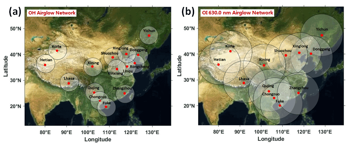
Figure 1 (a) OH airglow all-sky imager network (15 stations). (b) Red-line (630 nm) airglow all-sky imager network (12 stations). The circles on the maps give the effective observation ranges of OH and red-line airglow imagers with diameters of about 800 and 1800 km, respectively.

2 Data and methods

2.1 Double-layer all-sky airglow imager network data

A DLAN, including a hydroxyl radical (OH) layer (∼ 87 km) and a layer of atomic oxygen emission at 630 nm (OI 630.0 nm) (∼ 250 km), was established over mainland China. The research aim of the DLAN is to explore the physical mechanism of vertical and horizontal propagation and the evolution of atmospheric waves in the middle and upper atmosphere triggered by severe disasters, such as typhoons, earthquakes, and tsunamis. The OH airglow network comprises 15 stations, including the first no-gap OH airglow all-sky imager network located in northern China (Xu et al., 2015). The OI 630.0 nm airglow network contains 12 stations. Each imager consists of a 1024 × 1024 pixel back-illuminated charge-coupled device (CCD) detector and a Nikon 16 mm f/2.8D fisheye lens with a 180^∘ field of view (FOV). The OI 630.0 nm imager is operated at the 3.0 nm bandwidth filter with a central wavelength of 630.0 nm. Observations using airglow optical remote sensing require only a few airglow imagers to cover a wide area, although it is limited by meteorological conditions. Moreover, airglow observations can be used to monitor multi-layer GW activities. Figure 1a and b illustrate the OH and OI 630.0 nm network station distribution maps, respectively, in China. The OI 630.0 nm network covers nearly all of mainland China. Furthermore, the DLAN provides an excellent solution for studying the coupling processes between the mesosphere and thermosphere.

Several standard procedures were applied to raw airglow images, including star contamination subtraction, flat fielding to remove the van Rhijn effect, and atmospheric extinction (Li et al., 2011). The GW structure was retrieved by taking the deviation of each processed image from a half-hour running-average window image. Finally, the images were projected onto Earth's surface using the standard star map software and the altitude of the airglow layer (Garcia et al., 1997). The altitudes of the OH and OI 630.0 nm emission layers were set to approximately 87 and 250 km, respectively.

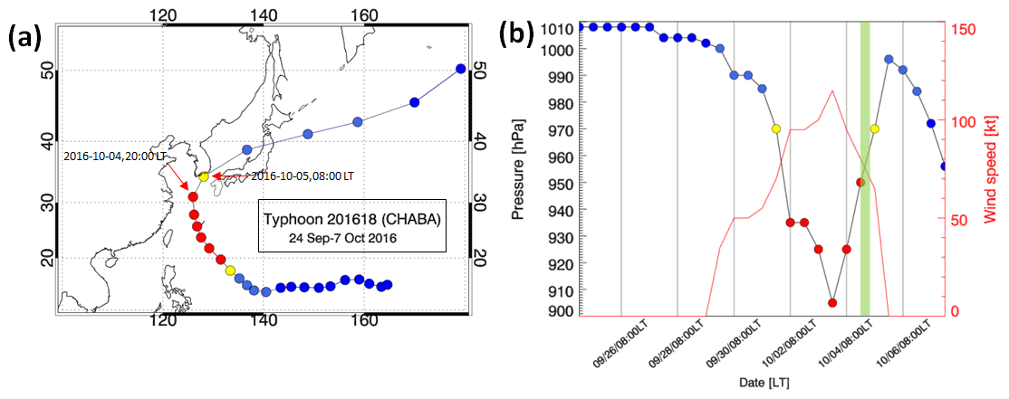
Figure 2 (a) The track of Typhoon Chaba is denoted by dots from 24 September to 7 October 2016 every 12 h (date format: year-month-day, hour). (b) Central pressure of Typhoon Chaba corresponding to the tracks in (a) (date format: month/day/hour). The red line denotes the maximum sustained wind speed. The green shadow band denotes the time of ground-based airglow observation from 20:00 to 04:00 LT during the night of 4–5 October 2016.

2.2 Development of Typhoon Chaba

Typhoon Chaba (2016) developed in the northwestern Pacific on 24 September 2016, and its track is shown in Fig. 2a. Initially, it moved westward and then turned northwestward on 30 September. The central pressure in the eye of the typhoon and the maximum wind speed are shown in Fig. 2b. On 3 October 2016 at 20:00 LT, the typhoon was in the mature stage with a minimum central pressure of 905 hPa and maximum sustained winds of approximately 59 m s⁻¹. The typhoon moved northward on 4 October 2016 at 02:00 LT until 5 October 2016 at 02:00 LT. The typhoon continued moving towards the northeast and disappeared on 8 October 2016 at 02:00 LT. Consecutive satellite images of the typhoon from MTSAT-1R from 18:00 LT on 3 October 2016 to 00:00 LT on 5 October 2016 are shown in Fig. 3. MTSAT-1R, which belongs to the Japan Meteorological Agency, is part of the Geostationary Meteorological Satellite series. MTSAT-1R is located at around 140^∘ E and covers East Asia and the western Pacific region. The MTSAT-1R consists of four infrared channels (IR1, IR2, IR3, and IR4) and one visible channel (VIS). The MTSAT-IR1 was used in this study. The track of the typhoon was beyond the effective FOV of the OH network and at the edge of the effective FOV of the OI 630.0 nm network.

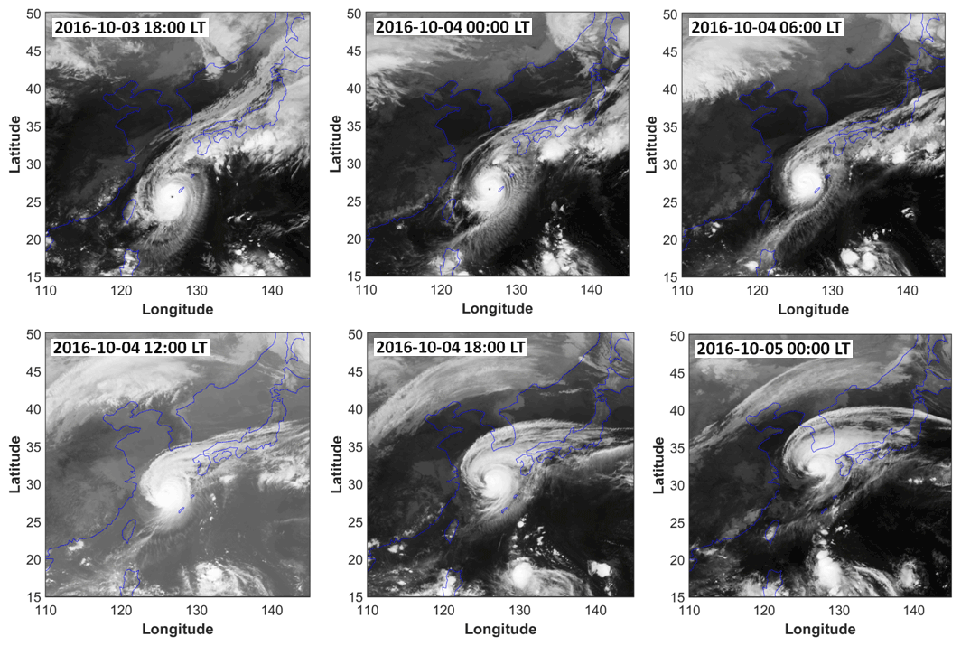
Figure 3 Consecutive satellite images of Typhoon Chaba from MTSAT-1R. The period is from 18:00 LT on 3 October to 00:00 LT on 5 October 2016, with an interval of 6 h.

2.3 ERA5 reanalysis data

ERA5 is a fifth-generation ECMWF atmospheric reanalysis that provides hourly data for many atmospheric and wave parameters. ERA5 is produced using a four-dimensional variational data assimilation algorithm based on Integrated Forecast System (IFS), with 137 hybrid sigma–pressure (model) levels in the vertical from 1000 to 0.01 hPa (0 to 80 km). More details of the model, data assimilation system, and observation data used to produce ERA5 were described by Hersbach et al. (2020). Horizontal reanalysis temperature and wind data with a pre-interpolated resolution of 0.25^∘ × 0.25^∘ and time resolution of 1 h were used in this study.

2.4 Ray-tracing model

We used a ray-tracing method to estimate the source location of the thermospheric secondary CGWs. The model was based on a dispersion relation that considers molecular viscosity and thermal diffusivity (Vadas, 2007), as shown in Eq. (1):

$$\begin{array}{}\text{(1)}& \begin{array}{rl}{m}^{\mathrm{2}}& ={\displaystyle \frac{k_{\mathrm{H}}^{\mathrm{2}}{N}^{\mathrm{2}}}{{\mathit{\omega }}_{Ir}^{\mathrm{2}}\left(\mathrm{1}+{\mathit{\delta }}_{+}+{\mathit{\delta }}^{\mathrm{2}}/\mathrm{Pr}\right)}}\\ & \times {\left[\mathrm{1}+{\displaystyle \frac{{\mathit{\nu }}^{\mathrm{2}}}{\mathrm{4}{\mathit{\omega }}_{Ir}^{\mathrm{2}}}}{\left(K^{\mathrm{2}}-{\displaystyle \frac{\mathrm{1}}{\mathrm{4}{H}^{\mathrm{2}}}}\right)}^{\mathrm{2}}{\displaystyle \frac{{\left(\mathrm{1}-{\mathrm{Pr}}^{-\mathrm{1}}\right)}^{\mathrm{2}}}{{\left(\mathrm{1}+{\mathit{\delta }}_{+}/\mathrm{2}\right)}^{\mathrm{2}}}}\right]}^{-\mathrm{1}}\\ & -k_{\mathrm{H}}^{\mathrm{2}}-{\displaystyle \frac{\mathrm{1}}{\mathrm{4}{H}^{\mathrm{2}}}},\end{array}\end{array}$$

where ${\mathit{\omega }}_{Ir}={\mathit{\omega }}_r-(ku+lv)$ is the intrinsic frequency (ω_r is ground-based frequency); $K^{\mathrm{2}}=k_{\mathrm{H}}^{\mathrm{2}}+m^{\mathrm{2}}$; $k_{\mathrm{H}}^{\mathrm{2}}=k^{\mathrm{2}}+l^{\mathrm{2}}$; H is the scale height; $\mathit{\nu }=\mathit{\mu }/\stackrel{\mathrm{‾}}{\mathit{\rho }}$ is the kinematic viscosity, where μ is the molecular viscosity and $\stackrel{\mathrm{‾}}{\mathit{\rho }}$ is the background density; $\mathit{\delta }=\mathit{\nu }m/H{\mathit{\omega }}_{Ir}$, ${\mathit{\delta }}_{+}=\mathit{\delta }$(1+ Pr ⁻¹), where Pr is the Prandtl number; and k, l, and m are the zonal, meridional, and vertical wave number components of the GW, respectively. The horizontal wavelength (k_H) of the CGW was obtained from the ground-based airglow observations; $N^{\mathrm{2}}=\left(g/T\right)\left(\mathrm{d}T/\mathrm{d}z+g/c_{\mathrm{p}}\right)$ is the square of the Brunt–Väisälä frequency, where g is the gravitational acceleration, T is the background temperature, and c_p is the specific heat at constant pressure. The background temperature T and density $\stackrel{\mathrm{‾}}{\mathit{\rho }}$ were obtained from the NRLMSISE-00 (Picone et al., 2002). The group velocity of the wave packet is formalized by Eq. (2):

$$\begin{array}{}\text{(2)}& c_{gi}=\mathrm{d}{x}_i/\mathrm{d}t=\partial {\mathit{\omega }}_{Ir}/\partial k_i+V_i,\end{array}$$

where V_i (u, v, w) is the background wind, which was obtained from the Horizontal Wind Model 14 (Drob et al., 2015), and w is the vertical wind velocity, which was neglected. In this study, we assume that the background wind field is independent of time, so ground-based frequency ω_r remains constant along a ray's path (Lighthill, 1978). However, the actual wind field changes with time, which may lead to deviation between the ray-tracing results and the wave source locations.

Using Eqs. (1)–(2), we yield the ground-based (zonal, meridional, and vertical) group velocity equation as follows (Vadas and Fritts, 2005):

$$\begin{array}{}\text{(3)}& \begin{array}{rl}{c}_{gx}& ={\displaystyle \frac{k}{{\mathit{\omega }}_{Ir}B}}\left[{\displaystyle \frac{N^{\mathrm{2}}\left(m^{\mathrm{2}}+\mathrm{1}/\mathrm{4}{H}^{\mathrm{2}}\right)}{{\left(K^{\mathrm{2}}+\mathrm{1}/\mathrm{4}{H}^{\mathrm{2}}\right)}^{\mathrm{2}}}}\right.\\ & \left.-{\displaystyle \frac{{\mathit{\nu }}^{\mathrm{2}}}{\mathrm{2}}}{\left(\mathrm{1}-{\mathrm{Pr}}^{-\mathrm{1}}\right)}^{\mathrm{2}}\left(K^{\mathrm{2}}-{\displaystyle \frac{\mathrm{1}}{\mathrm{4}{H}^{\mathrm{2}}}}\right){\displaystyle \frac{\left(\mathrm{1}+{\mathit{\delta }}_{+}+{\mathit{\delta }}^{\mathrm{2}}/\mathrm{Pr}\right)}{{\left(\mathrm{1}+{\mathit{\delta }}_{+}/\mathrm{2}\right)}^{\mathrm{2}}}}\right]+u,\end{array}\end{array}$$

$$\begin{array}{}\text{(4)}& \begin{array}{rl}{c}_{gy}& ={\displaystyle \frac{l}{{\mathit{\omega }}_{Ir}B}}\left[{\displaystyle \frac{N^{\mathrm{2}}\left(m^{\mathrm{2}}+\mathrm{1}/\mathrm{4}{H}^{\mathrm{2}}\right)}{{\left(K^{\mathrm{2}}+\mathrm{1}/\mathrm{4}{H}^{\mathrm{2}}\right)}^{\mathrm{2}}}}\right.\\ & \left.-{\displaystyle \frac{{\mathit{\nu }}^{\mathrm{2}}}{\mathrm{2}}}{\left(\mathrm{1}-{\mathrm{Pr}}^{-\mathrm{1}}\right)}^{\mathrm{2}}\left(K^{\mathrm{2}}-{\displaystyle \frac{\mathrm{1}}{\mathrm{4}{H}^{\mathrm{2}}}}\right){\displaystyle \frac{\left(\mathrm{1}+{\mathit{\delta }}_{+}+{\mathit{\delta }}^{\mathrm{2}}/\mathrm{Pr}\right)}{{\left(\mathrm{1}+{\mathit{\delta }}_{+}/\mathrm{2}\right)}^{\mathrm{2}}}}\right]+v,\end{array}\end{array}$$

$$\begin{array}{}\text{(5)}& \begin{array}{rl}{c}_{gz}& ={\displaystyle \frac{\mathrm{1}}{{\mathit{\omega }}_{Ir}B}}\left\{m\left[-{\displaystyle \frac{K_H^{\mathrm{2}}{N}^{\mathrm{2}}}{{\left(K^{\mathrm{2}}+\mathrm{1}/\mathrm{4}{H}^{\mathrm{2}}\right)}^{\mathrm{2}}}}\right.\right.\\ & -{\displaystyle \frac{{\mathit{\nu }}^{\mathrm{2}}}{\mathrm{2}}}{\left(\mathrm{1}-{\mathrm{Pr}}^{-\mathrm{1}}\right)}^{\mathrm{2}}\left(K^{\mathrm{2}}-{\displaystyle \frac{\mathrm{1}}{\mathrm{4}{H}^{\mathrm{2}}}}\right){\displaystyle \frac{\left(\mathrm{1}+{\mathit{\delta }}_{+}+{\mathit{\delta }}^{\mathrm{2}}/\mathrm{Pr}\right)}{{\left(\mathrm{1}+{\mathit{\delta }}_{+}/\mathrm{2}\right)}^{\mathrm{2}}}}\\ & \left.\left.+{\displaystyle \frac{{\mathit{\nu }}^{\mathrm{4}}{\left(\mathrm{1}-{\mathrm{Pr}}^{-\mathrm{1}}\right)}^{\mathrm{4}}}{\mathrm{16}{H}^{\mathrm{2}}{\mathit{\omega }}_{Ir}^{\mathrm{2}}}}{\displaystyle \frac{{\left(K^{\mathrm{2}}-\mathrm{1}/\mathrm{4}{H}^{\mathrm{2}}\right)}^{\mathrm{2}}}{{\left(\mathrm{1}+{\mathit{\delta }}_{+}/\mathrm{2}\right)}^{\mathrm{3}}}}-{\displaystyle \frac{{\mathit{\nu }}^{\mathrm{2}}}{\mathrm{Pr}{H}^{\mathrm{2}}}}\right]-{\displaystyle \frac{{\mathit{\nu }}_{+}{\mathit{\omega }}_{Ir}}{\mathrm{2}H}}\right\},\end{array}\end{array}$$

where

$$\begin{array}{rl}B& =\left[\mathrm{1}+{\displaystyle \frac{{\mathit{\delta }}_{+}}{\mathrm{2}}}+{\displaystyle \frac{{\mathit{\delta }}^{\mathrm{2}}{\mathit{\nu }}^{\mathrm{2}}}{\mathrm{16}{\mathit{\omega }}_{Ir}^{\mathrm{2}}}}{\left(\mathrm{1}-{\mathrm{Pr}}^{-\mathrm{1}}\right)}^{\mathrm{4}}{\displaystyle \frac{{\left(K^{\mathrm{2}}-\mathrm{1}/\mathrm{4}{H}^{\mathrm{2}}\right)}^{\mathrm{2}}}{{\left(\mathrm{1}+{\mathit{\delta }}_{+}/\mathrm{2}\right)}^{\mathrm{3}}}}\right],\\ {\mathit{\nu }}_{+}& =\mathit{\nu }\left(\mathrm{1}+{\mathrm{Pr}}^{-\mathrm{1}}\right).\end{array}$$

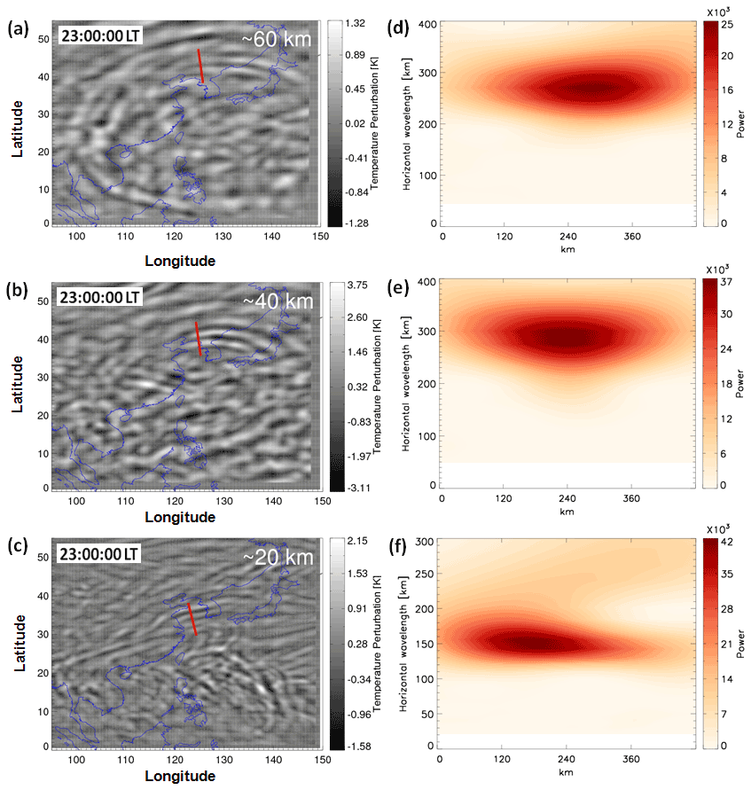
Figure 4 Temperature perturbations at (a) ∼ 60 km, (b) ∼ 40 km, and (c) ∼ 20 km at 23:00 LT on 4 October 2016 derived from ERA5 reanalysis. (d) Wavelet power spectrum along the red line in (a), (e) wavelet power spectrum along the red line in (b), and (f) wavelet power spectrum along the red line in (c).

3 Results

3.1 Propagation of typhoon-induced CGWs in the stratosphere

We extracted the stratospheric CGW excited by the typhoon from ERA5 reanalysis. Figure 4a, b, and c show the multi-layer temperature perturbations at approximately 60, 40, and 20 km at 23:00 LT, retrieved from the ERA5 reanalysis on 4 October 2016, respectively. Temperature perturbations were calculated by subtracting the background with a 7 × 7 grid point running mean at 20 km and 17 × 17 grid point running mean at 40 and 60 km. We found that the temperature disturbance was about ± 1.5–2 K at 20 km and ± 3–4 K at 40 km. Using the ECMWF reanalysis data, Kim et al. (2009) reported a similar temperature disturbance (± 4 K) at 40 km altitude. Becker et al. (2022) showed that typical temperature perturbation amplitudes simulated by the High Altitude Mechanistic general Circulation Model were ± 1–2 K in the wintertime lower stratosphere, as well as ± 5 K in the stratopause region. However, the temperature disturbance at 60 km in ERA5 was only ± 1.3 K and did not increase with increasing altitude, which may be caused by this altitude being well within the sponge layer of the reanalysis model. Figure 4d, e, and f show the corresponding wavelet analysis contours of the red line in Fig. 4a, b, and c. The expansion area of CGW at the height of 20 km (Fig. 4c) was small, and the horizontal wavelength was approximately 150 km from Fig. 4f. The CGWs were present over a large area of 0–50^∘ N, 100–150^∘ E at approximately 60 km. The distance of the CGWs, extending from the centre of the circle, ranged from 500 km (at approximately 20 km height) to 3000 km (at approximately 60 km height), which suggests that a larger-scale CGW arrives earlier at higher altitudes (faster vertical group velocities) than the smaller-scale waves (Vadas and Azeem, 2021). The ERA5 reanalysis data were utilized for characterizing the scale of the CGWs and indicated no small-scale fluctuation. According to the wavelet analysis of Fig. 4d and e, the horizontal wavelengths of the northward propagating CGW at 60 km (Fig. 4a) and 40 km (Fig. 4b) were approximately 265 and 290 km, respectively.

3.2 Propagation of typhoon-induced CGWs in the mesosphere

As the typhoon moved along the coast of China, CGWs were identified at 10 stations in the OH network. Animation 1 shows that CGWs were observed by the OH airglow network from 20:00–04:00 LT (the detailed data can be downloaded from the Supplement, https://doi.org/10.5446/55348). As the weather conditions in northern China during the study period were better than those in southern China, we identified clearer wave structures at the northern stations than at the southern stations. Nevertheless, circular wave structures were visible for brief clear weather intervals at the Zhangzhou, Qujing, and Chongzuo stations. The CGWs in the mesopause region extended to 2500 km, thereby nearly covering the effective FOV of the OH airglow network.

Figure 5 OH airglow emission perturbations induced by CGWs observed by the OH airglow imager network at (a) 23:21 LT, (b) 23:36 LT, and (c) 23:53 LT on 4 October 2016. (d) Wavelet power spectrum along the red line in (a), (e) wavelet power spectrum along the red line in (b), and (f) wavelet power spectrum along the red line in (c).

As long as the CGWs do not encounter the critical layer or break, the CGWs generated in the lower atmosphere can propagate to the OH airglow layer. Through the propagation group velocity, we can determine the propagation time to the OH layer. A single dominant horizontal wavelength is seen at each altitude of 20, 40, and 60 km in the ERA5 reanalysis. In contrast, the horizontal scales of the CGW obtained by the OH airglow network were diverse, ranging from approximately 30 to 300 km. More importantly, we found some CGWs in the OH airglow layer, which were close to the CGW wavelengths at 20, 40, and 60 km altitudes. To verify whether the same wave was propagated from the reanalysis data layer to the OH layer, we used the group velocity to estimate the time when the CGW at the altitudes of 20, 40, and 60 km reached the OH airglow layer. The times required for the CGW in the three-layer disturbance diagram in Fig. 4a, b, and c to reach the OH layer were approximately 21, 36, and 53 min. Therefore, the times when the CGWs visible in ERA5 at 60, 40, and 20 km would reach the OH airglow layer are approximately 23:21, 23:36, and 23:53 LT as shown in Fig. 5a, b, and c, respectively. The wavelet analysis of Fig. 5f showed that the horizontal wavelength of the CGW in the OH airglow layer (Fig. 5c) is approximately 156 km; the observed period is approximately 23 min; and the horizontal speed is approximately 113 m s⁻¹, which is similar to the dominant horizontal wavelength of the CGWs in the ERA5 reanalysis at 20 km altitude. Similarly, the horizontal wavelengths of the CGW in the OH airglow layers (Fig. 5a and b) were approximately 270 and 295 km from the wavelet analysis of Fig. 5d and e, which is similar to the dominant horizontal wavelength of the CGWs in the ERA5 reanalysis at 60 and 40 km altitudes. This suggests that the same CGW event can be perfectly tracked over different altitudes and that the CGWs in the mesosphere propagated upward from the stratosphere.

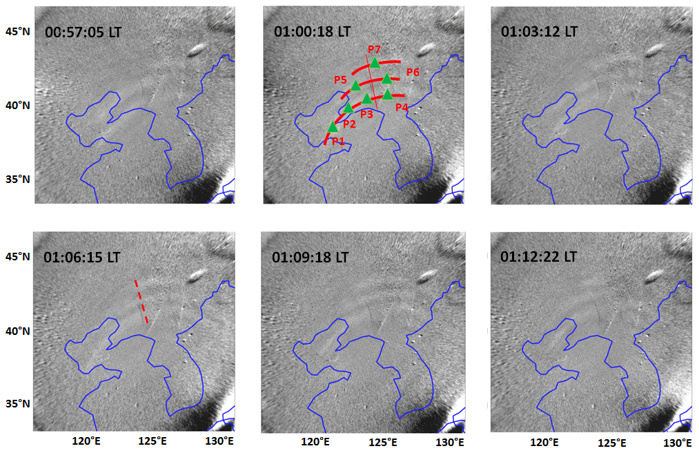
Figure 6 Time sequence of OI 630.0 nm airglow emission perturbation images observed by the Donggang station from 00:57:05–01:12:22 LT on the night of 4 October 2016. Green triangles (P1–P7) in the red arcs are used as ray-tracing sampling points. The blue line in each panel represents the coastline.

Figure 7 Wavelet power spectrum along the red line at 01:00:18 LT in Fig. 6.

3.3 How typhoon-induced CGWs propagate to the thermosphere

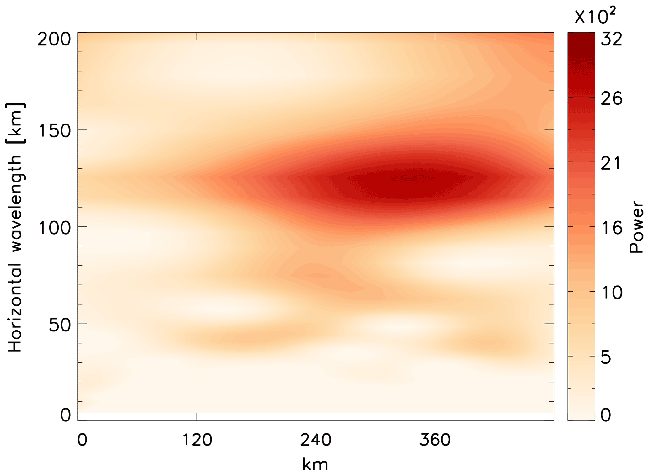
Figure 6 shows the time sequence of the OI 630.0 nm airglow images from 00:57:05 to 01:12:22 LT on the night of 4 October 2016. Three curved phase fronts are clearly visible. The wave packet observed in the OI 630 nm airglow was quasi-monochromatic. According to the wavelet analysis spectrum in Fig. 7, the horizontal wavelength was approximately 120 km. The observed wave period and phase velocity were 10 min and 200 m s⁻¹, respectively. The horizontal wavelength was somewhat less than the typhoon-induced concentric travelling ionosphere disturbances with a horizontal wavelength from 160 to 200 km in the GNSS-TEC (global navigation satellite system–total electron content) network as reported by Chou et al. (2017). The CGW observed in the OI 630.0 nm airglow had a much faster phase speed and shorter period than that observed in the mesosphere, which indicates that its propagation trajectory was relatively vertical. This means that they will not propagate as far horizontally as the CGWs noted as dominant in the OH layer. Indeed, compared with the long-distance extension of the CGWs in the mesosphere, the horizontal propagation distance of the CGWs in the thermosphere was only 600 km from OI 630.0 nm network observation. Vadas and Crowley (2010) showed that thermospheric GWs may be secondary GWs generated by the breaking of primary GWs in the mesosphere and thermosphere. We argue that the thermospheric CGW observed by the OI 630.0 nm airglow imager was not directly generated by the typhoon but rather a secondary GW. To test this hypothesis, backward-ray-tracing analysis was applied. In this way, we determined the source of the CGW observed in the thermosphere.

Figure 8 (a) Wind profiles along the seven ray-tracing paths. (b) Ray paths of the wave starting from the seven sampling points in Fig. 6. (c) Horizontal area distribution of the terminal positions of the seven backward-traced trajectories. Error bars give the standard deviation for each point from the starting altitudes of 240, 250, and 260 km.

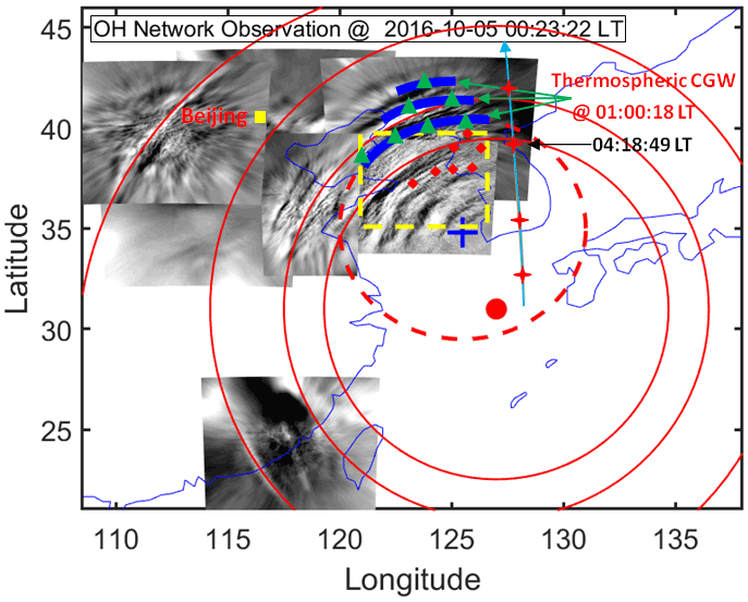
Figure 9 Double-layer CGW-superimposed graph. The blue arcs represent the thermospheric CGW observed at 01:00:18 LT. The dotted circle represents the approximately fitting blue arcs. The blue cross marks the centre of the circle. The solid circles represent the approximately fitting CGWs observed by the OH airglow network. The red dot marks the centre of the circles. The green triangles and red diamonds represent the trace start and termination points, respectively. The red crosses represent the sounding footprints of the TIMED–SABER (Thermosphere Ionosphere Mesosphere Energetics and Dynamics satellite's Sounding of the Atmosphere using Broadband Emission Radiometry instrument) measurements. The yellow box marks the location of the meteor radar station.

We sampled seven points (green triangles) on circular wavefronts (red arcs in Fig. 6) at 01:00:18 LT as the starting point for backward ray tracing. The starting height of the backward ray tracing was 250 km. The profile of the winds used in the ray tracing is shown in Fig. 8a. The ray-tracing trajectories of the seven sampling points are shown in Fig. 8b. We used the following criterion to terminate the ray tracing: the square of the vertical wavenumber should be negative. We started the ray tracing at heights of 240, 250, and 260 km and analysed the results. The maximum uncertainty of the horizontal change of the ray-tracing termination point caused by different starting heights was approximately ± 0.36^∘ in latitude and ± 0.17^∘ in longitude (see Fig. 8c). Subsequently, seven backward-traced trajectories took 37 min and terminated at an altitude of approximately 95 km, thereby indicating that a reflection layer was encountered. According to linear theory, this suggests that the thermospheric CGW could not have come from below 95 km. The thermospheric GW must have been generated at any altitude between 95 km and the altitude of the OI 630.0 nm airglow. In other words, the CGW observed in the thermosphere was excited after approximately 00:23 LT. Figure 9 presents the CGWs observed by the OH airglow network at 00:23:22 LT. We superimposed the thermospheric CGWs along with the starting ray-tracing points (green triangles) reproduced from Fig. 6, as well as the backward-ray-tracing termination points (red diamonds) on the OH airglow observation images. The dotted circle represents the approximate fitting thermospheric CGW fronts. The centre of the circle is marked by a blue cross. Compared with the single-scale wave observed in the OI 630.0 nm layer, multi-scale CGWs were visible from OH network observations. We found that the termination points of ray tracing almost fell above the mesopause region. This suggests that the CGW observed in the thermosphere did not directly originate from the typhoon but may have emerged due to the dissipation and/or nonlinear processes of a typhoon-induced CGW in the mesopause region. However, the backward-tracing terminal positions (red diamonds in Fig. 9) did not coincide with the fitting circle centre position (blue cross in Fig. 9). Nevertheless, according to numerical simulation work by Vadas et al. (2009), large winds can shift the apparent centre of concentric rings from the location of the convective plume. Indeed, we found strong southward winds at 100 to 140 km (with a peak value of 50 m s⁻¹ at 150 km altitude) and 160 to 220 km (with a peak value of 25 m s⁻¹ at 175 km altitude) altitudes (right panel of Fig. 8a). So the centre of the thermospheric CGW can be shifted southward from the location of the thermospheric CGW sources in the mesopause region. For the zonal wind, the westward wind dominated from the upper mesosphere to the thermosphere (left panel of Fig. 8a). Similarly, the thermospheric CGW centre position shifted westward. Therefore, the assumed centre (blue cross) of the partial concentric ring GWs (blue arcs) actually shifted to the southwest from the real source location, which may explain why the ray-tracing result for the assumed GW source did not match the fitting centre of the partial concentric ring thermospheric GWs. Another possible mechanism is that the wave phase speeds are accelerated by accelerating background winds. As mentioned above, the ground-based frequency ω_r remains constant along a ray's path assuming the background wind field is independent of time (Lighthill, 1978). However, the transient effect (time derivatives of the background wind components giving rise to the time derivative of the frequency for a particular ray) may cause the phase speeds to be accelerated, which may lead to the ray-tracing results not matching the real locations. As the ray-tracing model used in this study depended on the linear theory and did not consider the wave–wave and wave–mean flow interactions and tunnelling, the ray-tracing results were limited and should also be taken into consideration carefully.

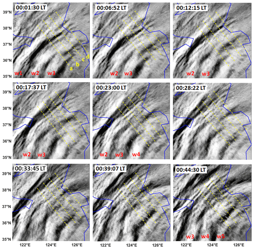
Figure 10 Time sequence of OH airglow emission perturbation images observed by the Rongcheng station from 01:01:30–00:44:30 LT on the night of 4 October 2016. w1–w5 denote the wavefronts of the CGW. The blue line in each panel represents the coastline.

4 Discussion

Figure 10 presents a time sequence of OH airglow images in the range marked by the yellow dotted rectangle in Fig. 9. The images were retrieved from the Rongcheng station from 00:01:30 to 00:44:30 LT on the night of 4 October 2016. At 00:01:30 LT, three distinct curved wavefronts with horizontal wavelengths of approximately 96 km were identified. Interestingly, wavefronts w2 and w3 collided and connected in the northeast, indicating that wave–wave nonlinear interactions may have occurred.

Figure 11 Time series of the averaged OH image slices perpendicular to the wavefronts as marked by four yellow dotted lines (a, b, c, and d) in Fig. 10. The wavefronts propagate from left to right. The red arrows mark the evolution of the wavefront peak.

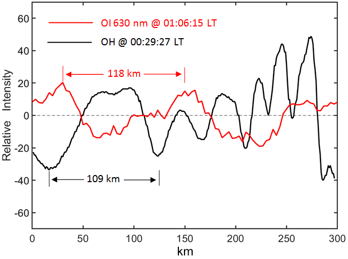
Figure 12 OH (black) and OI 630 nm (red) airglow relative-intensity variations. The OH relative-intensity variation is obtained as in Fig. 11. The OI 630 nm relative-intensity variation is from the red dotted line in Fig. 6 at 01:06:15 LT.

Figure 11 shows the time series of the OH image slices perpendicular to the wavefronts (w1–w5). A dominant wavelength of approximately 150 km can be confirmed at 00:00:25 LT. We found a significant attenuation of the amplitude from 00:00:25 to 00:17:37 LT. At 00:00:25 LT, the relative average power was 2.3 ×10³, and the amplitude decreased gradually with time. At 00:17:37 LT, the average power decreased to 0.15 ×10³. We also identified the generation of approximately 110 km and 20–50 km small-scale waves from the larger scales, which may be caused by wave–wave nonlinear interactions and/or wave breaking. We overlaid the OI 630 nm airglow relative-intensity variation on the OH airglow variation, and Fig. 12 shows OH and OI 630 nm airglow relative-intensity variations. The OH plot was obtained at 00:29:27 LT, as well as the OI 630 nm plot at 01:06:15 LT. The time interval of 37 min was calculated by the above ray-tracing analysis. We obtained similar-scale fluctuations in the two airglow layers. The horizontal wavelength of the wave obtained by the OI 630 nm airglow layer was approximately 118 km. The OH airglow layer has also obtained near-scale fluctuations with wavelengths of approximately 109 km. These waves could be the same waves seen in the thermosphere. Therefore, the CGW in the thermosphere may come from breaking or nonlinear processes of primary gravity waves.

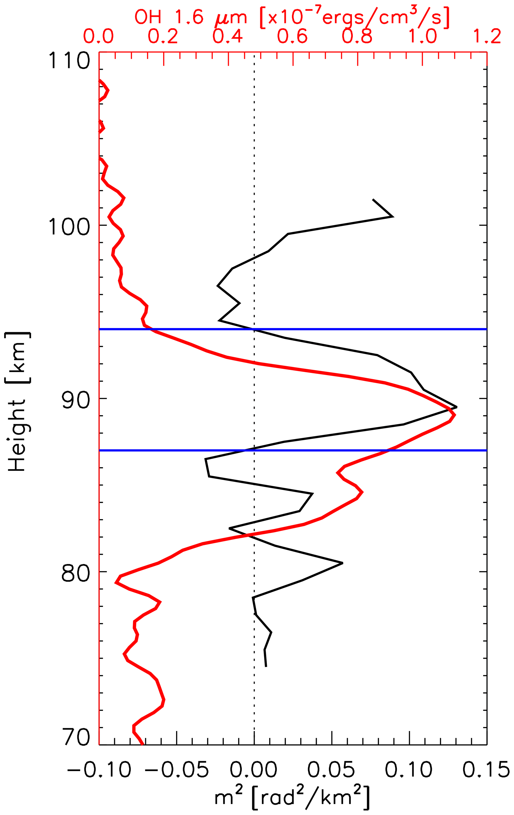
Figure 13 Square of vertical wave number m² profile (black) derived from the temperature from the TIMED–SABER measurement location at 04:18:49 LT and the meteor radar wind from the Beijing station marked in Fig. 9. The red line represents the OH 1.6 µm emission intensity obtained by the TIMED–SABER. The horizontal blue lines represent the top and bottom boundaries of the duct region.

Note that wave amplitude fluctuations can also result from the transient nature of the wave packet. The propagation state can be studied by using the dispersion relationship with the GW. However, the dissipation region of the CGW lacks the real-time background temperature and wind field. In this context, the limb viewing of the Sounding of the Atmosphere using Broadband Emission Radiometry (SABER) instrument on the Thermosphere Ionosphere Mesosphere Energetics and Dynamics (TIMED) satellite can be beneficial because it occurred near the wave-dissipation region; however, the time lag was close to approximately 4 h. Background wind field data were obtained from an ATRAD MDR6 all-sky VHF (very high-frequency) meteor radar at the Beijing station. We further examined the dispersion relationship of the GW, thereby shedding some light on the possible propagation state of dissipative waves. Figure 13 presents the square of vertical wave number m² profile derived from the Beijing meteor radar wind and the temperature from the TIMED–SABER measurement location at 04:18:49 LT, as marked in Fig. 9. The wave parameters used were from the wavefronts (w1–w5) in Fig. 10. The average horizontal wavelength was approximately 96 km, and the average observed phase velocity is approximately 90 m s⁻¹. We identified a clear duct (from 87 to 94 km) near the peak of the OH airglow layer. Note that the duct can control the horizontal propagation of the CGW. This implies that the CGW may indeed be dissipated. In contrast, the upper boundary of the duct coincided with the height of the ray-tracing termination area mentioned above. During wave dissipation, momentum deposition occurs in the background atmosphere and can produce body forces that stimulate secondary GWs (Fritts et al., 2006; Chun and Kim, 2008; Smith et al., 2013; Vadas et al., 2018; Heale et al., 2020). In addition, secondary waves can be generated by momentum transferred nonlinearly from the primary wave mode to harmonics or subharmonics (Snively, 2017). Local momentum flux divergence associated with wave breaking, vortex generation, and wave interactions can also generate secondary GWs (Fritts et al., 2006).

5 Summary

In this study, a DLAN was used to capture CGWs over China that were excited by Typhoon Chaba (2016). As Typhoon Chaba (2016) moved northward along the coast of the Chinese mainland and developed to a mature stage, remarkable multi-layer CGW features produced by the Typhoon from near the ground to a height of 250 km were observed by ERA5 reanalysis and the airglow network. We applied the MTSAT-1R observations, ERA5 reanalysis data, and backward ray tracing to quantitatively describe the physical mechanism of typhoon-generated CGWs propagating throughout the stratosphere, mesosphere, and thermosphere.

The temperature disturbance was approximately ± 1.5–2 K at 20 km and ± 3–4 K at 40 km. However, the temperature disturbance (± 1.3 K) at 60 km altitude did not increase with a further increase in altitude, which may be caused by the sponge layer effect. Using reanalysis of multi-layer temperature disturbance, group velocity of gravity wave, and wavelet analysis, we demonstrated that the CGWs in the mesopause region were excited directly by the typhoon.

Due to the observational limitations, a backward-ray-tracing theory was used to connect GWs in the upper mesosphere to GWs in the thermosphere at about 250 km. We found that the termination points of ray tracing of the thermospheric CGW almost fell above the mesopause region. Backward-ray-tracing analysis and the CGW evolution process observed by the OH network suggested that the CGW observed in the thermosphere did not directly originate from the typhoon but may have emerged due to dissipation and/or nonlinear processes of typhoon-induced CGWs in the mesopause region. Airglow network observations combined with numerical simulation to study the generation of secondary wave in detail will be carried out in the future.