the Creative Commons Attribution 4.0 License.
the Creative Commons Attribution 4.0 License.
 | 16 Sep 2022
Impact of present and future aircraft NOx and aerosol emissions on atmospheric composition and associated direct radiative forcing of climate
Etienne Terrenoire
Didier A. Hauglustaine
Yann Cohen
Anne Cozic
Richard Valorso
Franck Lefèvre
Sigrun Matthes
Aviation NOx emissions not only have an impact on global climate by changing ozone and methane levels but also contribute to the deterioration of local air quality. A new version of the LMDZ-INCA global model, including chemistry of both the troposphere and the stratosphere and the sulfate-nitrate-ammonium cycle, is applied to re-evaluate the impact of aircraft NOx and aerosol emissions on climate. The results confirm that the efficiency of NOx to produce ozone is very much dependent on the injection height; it increases with the background methane and NOx concentrations and with decreasing aircraft NOx emissions. The methane lifetime variation is less sensitive to the location of aircraft NOx emissions than the ozone change. The net NOx radiative forcing (RF) (O3+CH4) is largely affected by the revised CH4 RF formula. The ozone positive forcing and the methane negative forcing largely offset each other, resulting in a slightly positive forcing for the present day. However, in the future, the net forcing turns to negative, essentially due to higher methane background concentrations. Additional RFs involving particle formation arise from aircraft NOx emissions since the increased hydroxyl radical (OH) concentrations are responsible for an enhanced conversion of SO2 to sulfate particles. Aircraft NOx emissions also increase the formation of nitrate particles in the lower troposphere. However, in the upper troposphere, increased sulfate concentrations favour the titration of ammonia leading to lower ammonium nitrate concentrations. The climate forcing of aircraft NOx emissions is likely to be small or even switch to negative (cooling), depending on atmospheric NOx or CH4 future background concentrations, or when the NOx impact on sulfate and nitrate particles is considered. However, large uncertainties remain for the NOx net impact on climate and in particular on the indirect forcings associated with aerosols, which are even more uncertain than the other forcings from gaseous species. Hence, additional studies with a range of models are needed to provide a more consolidated view. Nevertheless, our results suggest that reducing aircraft NOx emissions is primarily beneficial for improving air quality.
- Article
(5071 KB) - Full-text XML
-
Supplement
(3825 KB) - BibTeX
- EndNote


Air traffic emissions represent a sizeable contribution to global anthropogenic climate change (Lee et al., 2021) and also to regional surface air pollution, particularly around airports (Yim et al., 2015). Aircraft release into the atmosphere not only gaseous compounds such as carbon dioxide (CO2), nitrogen oxides (NOx), hydrocarbons (HC), sulfur dioxide (SO2) and water vapour (H2O), but also particulate material composed of ice crystals, soot particles (black carbon, BC) and sulfates (SO4) (e.g. Kärcher, 2018; Lee et al., 2021). There is a wide range of spatial and temporal scales associated with atmospheric perturbations due to aircraft emissions. It ranges from the local and plume scales for chemical species, aerosols, and contrail-cirrus formation to the global scale for methane and carbon dioxide perturbations; and from a few minutes after emission up to several decades (Brasseur et al., 2016). Evaluating the global chemical and climate perturbations associated with aircraft emissions therefore appears to be a complex issue.
Due to this range of scales as well as the different nature of the perturbations of the climate system involved, a distinction is usually made between the CO2 and the non-CO2 climate impacts of aviation. These climate forcings were recently reassessed by Lee et al. (2021). For 2018, the net aviation effective radiative forcing (ERF) of historic aviation emissions until 2018 was estimated to 101 mW m−2 in this recent study with major contributions from contrail cirrus (57.4 mW m−2 or 57 % of the total forcing), CO2 (34.3 mW m−2, 34 %), and NOx (17.5 mW m−2, 17 %). Non-CO2 terms represent a net positive forcing that accounts for more than half (66 %) of the aviation total RF of climate. In contrast to the CO2 forcing which is relatively well determined, except for some methodological issues (Terrenoire et al., 2019; Ivanovich et al., 2019; Boucher et al., 2021), non-CO2 forcing terms contribute about 8 times more than CO2 to the uncertainty in the aviation total forcing (Lee et al., 2021).
From these non-CO2 climate forcings associated with aircraft emissions, nitrogen oxides (NOx) play a particular role. Indeed, they not only affect climate by changing the atmospheric concentration of two important greenhouse gases, i.e. ozone (O3) and methane (CH4) (e.g. Hauglustaine et al., 1994; Brasseur et al., 1998; Holmes et al., 2011; Myhre et al., 2011), but also have an impact on local air quality and human health, both through emissions in and around airports and from emissions at higher altitude affecting near-ground background concentrations (e.g. Barrett et al., 2010; Hauglustaine and Koffi, 2012; Cameron et al., 2017). For this reason, it has been assumed that emission standards for NOx emissions set by the International Civil Aviation Organization (ICAO) since the 1980s not only protected local air quality but also had co-benefits for climate change mitigation (Skowron et al., 2021). A technological difficulty faced by aircraft industry today is that reducing NOx emissions tends to increase fuel burn, hence resulting in increased CO2 emissions and a climate penalty (Freeman et al., 2018). There is however a possibility that technological development could simultaneously lead to the reduction of CO2 and NOx emissions (Prashanth et al., 2021). Hence, a better quantification of the aircraft NOx effect on climate is needed to determinate whether the climate effect of the CO2 increase linked to new technology could be compensated by the associated NOx reduction.
Emissions of NOx into the troposphere result in a short-term increased photochemical ozone production (resulting in a positive climate forcing or warming), and a long-term increased oxidation of atmospheric methane through reaction with the hydroxyl radical (OH; resulting in a negative climate forcing or cooling), as shown by Fuglestvedt et al. (1999) and Szopa et al. (2021). In addition, the aforementioned methane reduction leads to a long-term reduction in tropospheric O3 (cooling) and a long-term reduction in stratospheric H2O (cooling). In the lower troposphere, the net effect of NOx emissions is dominated by the increased methane destruction and a negative forcing is predicted. In the upper troposphere, at aircraft cruise altitudes, the ozone production is about 5 times more efficient per molecule of NOx emitted (e.g. Hauglustaine et al., 1994; Derwent et al., 2001; Hoor et al., 2009; Dahlmann et al., 2011) and a positive net RF of climate is generally associated with aircraft NOx emissions (e.g. Holmes et al., 2011; Myhre et al., 2011; Hoor et al., 2009; Søvde et al., 2014; Brasseur et al., 2016; Lee et al., 2021). Based on an in-depth literature assessment, Lee et al. (2021) provided the most recent estimate of these forcings and derived a net NOx RF from all emissions released by aviation of 17.5 (0.6, 28.5) mW m−2 in 2018, decomposed into a positive short-term tropospheric ozone forcing of 49.3 (32, 76) mW m−2 and a negative methane forcing of −34.9 (−65, −25.5) mW m−2. The aircraft NOx net RF of climate is positive, but this net effect is the sum of two forcings of opposite sign, distinct geographic distributions, and each of them associated with large uncertainties.
Recently, Skowron et al. (2021) reinvestigated the aircraft NOx climate forcing based on various future scenarios for both surface and aircraft NOx emissions using the MOZART-3 global chemistry–climate model (Kinnison et al., 2007). They found that in all their future (2050) simulations and even for “present-day” (2006) simulations under certain conditions, the net RF from aircraft NOx emissions could turn negative. This finding is essentially associated with the revised expression for methane direct RF from Etminan et al. (2016) which increases, for instance, the methane forcing by 24.5 % for a halving of its atmospheric concentration compared to previous formulations. However, another major uncertainty associated with the impact of NOx emissions on atmospheric composition arises from the non-linear character of the tropospheric chemistry. This feature makes the impact of aircraft NOx emissions dependent on the background atmospheric concentrations and hence sensitive to anthropogenic surface emissions of NOx, CO, and HCs or even to natural emissions such as lightning NOx (Holmes et al., 2011; Skowron et al., 2021). It also makes the impact of aircraft NOx emissions very dependent on the location of the emission and on the season (Stevenson et al., 2004; Stevenson and Derwent, 2009; Gilmore et al., 2013; Skowron et al., 2013; Søvde et al., 2014). Since the ozone production sensitivity differs from the methane destruction sensitivity, the positive short-term ozone forcing associated with aircraft NOx emissions can be overwhelmed by the methane negative forcing, providing a negative net radiative forcing of climate (Stevenson and Derwent, 2009; Skowron et al., 2021).
Other effects of aircraft NOx emissions, less accounted for in earlier studies, include the role played by tropospheric aerosols and in particular, the impact on secondary inorganic aerosols such as nitrates and sulfates (Unger, 2011; Pitari et al., 2015; Brasseur et al., 2016; Lund et al., 2017; Prashanth et al., 2022). Increased NOx emissions from aircraft indeed have the potential to form ammonium nitrate particles. However, the changes in oxidants and the direct emissions of SO2 by aircraft also increase the formation of sulfate particles with possible implications on nitrate concentrations (Unger et al., 2013; Righi et al., 2013, 2016). These indirect forcings associated with aircraft NOx emissions are however complex and need further investigation since they can provide additional negative direct forcings of climate. In order to account for the role played by secondary inorganic aerosols and other interactions involving gas-phase and aerosol chemistry, the global models used to assess the impact of aircraft NOx emissions need to include both gas-phase chemistry, tropospheric aerosols, and in particular, the role played by the sulfate-nitrate-ammonium cycle.
The aim of the present study is to provide a comprehensive and updated model-based analysis of the impact of aircraft NOx emissions on atmospheric composition and associated RF of climate. The LMDZ-INCA global model, including both tropospheric and stratospheric chemistry as well as tropospheric aerosols, is applied. An earlier and less mature version of this model was previously used by Koffi et al. (2010) and Hauglustaine and Koffi (2012), or in several model intercomparisons (Hoor et al., 2009; Hodnebrog et al., 2011, 2012; Myhre et al., 2011) in order to investigate the impact of NOx transport emissions on atmospheric composition and climate. This earlier version of the model only included tropospheric gas-phase chemistry and used a coarser vertical resolution. The new version of LMDZ-INCA used in this study allows us to revisit the impact of aircraft NOx emissions on ozone production, changes in oxidants, and methane destruction, but also its impact on the secondary inorganic aerosol distributions. These earlier studies will provide a point of comparison for this new assessment. This study not only focuses on the effect of aircraft NOx emissions but also includes aircraft SO2 and aerosols emissions in order to account for the effect of the sulfate-nitrate-ammonium cycle and considers the potential effect linked to heterogeneous chemistry. Similarly, the direct water vapour aircraft emission is also included in order to account for the role of stratospheric water vapour on atmospheric oxidants and is linked with the methane indirect effect on H2O.
Moreover, another aim of this paper is to investigate the sensitivity of the aircraft NOx net RF of climate to various mitigation options. Motivated by earlier work (e.g. Unger, 2011; Hodnebrog et al., 2012; Matthes et al., 2021; Skowron et al., 2021) we particularly assess the sensitivity of the NOx forcing to a variation of the aircraft emission injection height and to background (present versus future) atmospheric concentrations. Several scenarios are considered for the future in order to investigate low and high assumptions in air traffic growth and fuel-burn efficiencies. Other scenarios will also illustrate more specifically the impact of desulfurized jet fuel as a mitigation option or engines with ultra-low NOx combustor technology. For all these present-day and future (2050) scenarios, the changes in atmospheric composition are illustrated and the RFs of climate associated with NOx emissions (O3 and CH4 direct and indirect forcings) and aerosol direct effects are calculated.
The remainder of this paper is organized as follows: in Sect. 2, we present the aircraft emission inventories prepared and introduced in the global chemistry–climate model for both the present-day baseline simulation and for the future (2050) baseline and mitigation scenarios. In Sect. 3, we provide a description of the LMDZ-INCA chemistry–climate model used in this study along with a description of the RF calculations and modelling setup. Additionally, in Sect. 3, we summarize the model performance comparing the model results with ozone soundings and the In-service Aircraft for a Global Observing System's (IAGOS) measurements of ozone and carbon monoxide concentrations in the upper troposphere and lower stratosphere. In Sect. 4, we present the atmospheric composition perturbations associated with the present-day aircraft emissions, and in Sect. 5 the perturbations associated with future aircraft emissions under different scenarios. We then present the RF of climate associated with the changes in atmospheric composition in Sect. 6. Finally, in Sect. 7, we discuss conclusions drawn from this study.
The global three-dimensional and time-varying aircraft emission inventories used in this study are essentially based on the previous European Union (EU) projects: Reducing Emissions from Aviation by Changing Trajectories for the benefit of Climate (REACT4C; Matthes et al., 2012) and Quantifying the Climate Impact of Global and European Transport Systems (QUANTIFY; Lee et al., 2010). These inventories are based on the fuel-flow model PIANO (Project Interactive Analysis and Optimization) and the global emission model FAST (Future Aviation Scenario Tool) with air traffic movements coming from radar data for European and North American flights and the Official Airline Guide (OAG) database for the remaining global flight movements (Lee et al., 2009; Owen et al., 2010). For this specific study, the methodology used to derive emissions for the global chemistry–transport model LMDZ-INCA is further described in the following Sect. 2.1 for present-day baseline emissions and in Sect. 2.2 for the future (2050) emission scenarios.
2.1 Present-day baseline emissions
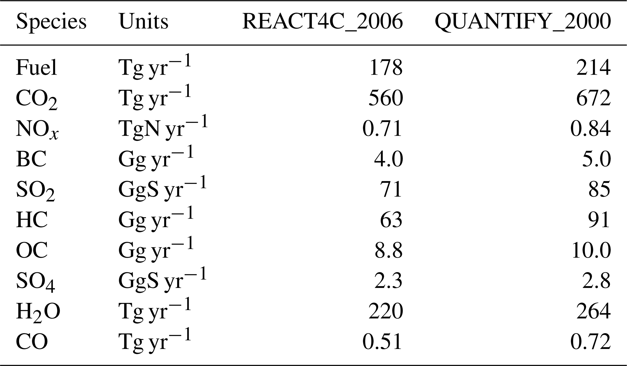
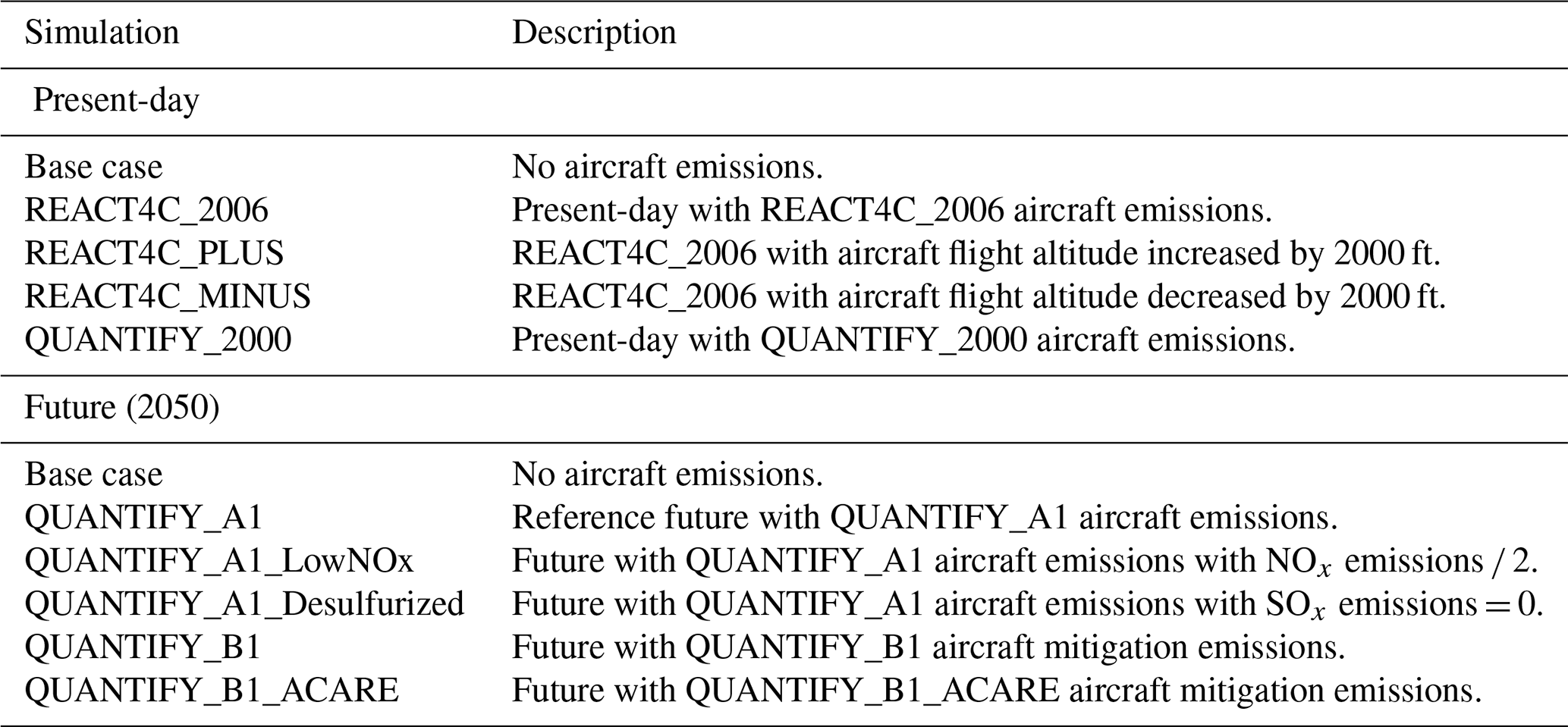
The aircraft emission inventory used for present-day baseline emissions is based on the EU project REACT4C (Matthes et al., 2012, 2021; Søvde et al., 2014; Grewe et al., 2014) and is representative of the year 2006. This inventory will be referred to as REACT4C_2006 in this paper. The REACT4C_2006 data include three-dimensional gridded distributions of kilometres travelled, fuel consumption, as well as CO2, NO2, and BC (soot) emissions. Flight data are derived from CAEP8 data using the “great circle distance” method corrected with the CAEP8 formula. This dataset is available on a latitude–longitude–altitude grid for 12 months with a horizontal resolution of and a 610 m vertical resolution. In this inventory, the global mean NOx emission index (EI) is 12.1 gNO2 kg−1 fuel (12.7 gNO2 kg−1 below 1800 m and 12.3 gNO2 kg−1 above 8400 m). For BC, the mean EI is 0.023 gBC kg−1 fuel (0.046 gBC kg−1 below 1800 m and 0.015 gBC kg−1 above 8400 m). Additional species are needed to run the global chemistry–transport model. For H2O, carbon monoxide (CO) and total non-methane HCs, we use the three-dimensional emissions from the AERO2K project inventory (Eyers et al, 2005). The EIs for these species are derived for the AERO2K vertical levels (500 ft vertical resolution) and interpolated onto the REACT4C vertical levels. Based on the REACT4C fuel burn, we then derive the H2O, CO, and HC three-dimensional and monthly emissions representative of the year 2006. For HC, we use the speciation given by the Federal Aviation Administration (FAA; 2009) in order to derive the emissions of the LMDZ-INCA model's individual HCs. For organic carbon (OC), SO2 and SO4, we use the mean EIs reported by Lee et al. (2010). For OC, Lee et al. (2010) provide a range of 0.0065–0.05 g kg−1. As was done by Balkanski et al. (2010) and Righi et al. (2016), we choose the highest EI value of 0.05 g kg−1 fuel and determine a maximum value for OC produced from aircraft. For SO2 and SO4, the mean EIs are respectively 0.8 and 0.04 g kg−1 fuel. From REACT4C_2006, we derive global EIs of 3.15 kgCO2 kg−1 fuel, 1.23 kgH2O kg−1 fuel, 3.25 gCO kg−1 fuel, and 0.405 gHC kg−1 fuel, which compare well to the EI and EI used in the recent review of Lee et al. (2021). They are somewhat lower than the EIs used in Lee et al. (2021) for BC (EIBC=0.03 gBC kg−1 fuel), NOx (EI gNO2 kg−1 fuel) and SO2 (EI g kg−1 fuel). Table 1 summarizes the total emissions for the baseline REACT4C_2006 inventory. Figure S1 shows the zonal and annual mean distribution of REACT4C_2006 fuel use, NO2, and BC emissions.
Table 1Total global aircraft emissions corresponding to the baseline REACT4C_2006 and QUANTIFY_2000 inventories.
The REACT4C_2006 inventory is chosen for the present-day baseline simulation since this inventory provides, in addition to the baseline emissions, two additional mitigation inventories. These mitigation scenarios based on the original REACT4C_2006 emissions were used in this study in order to investigate the sensitivity of the chemical perturbations and associated RFs to a cruise altitude variation (Søvde et al., 2014; Matthes et al., 2021). The REACT4C_PLUS corresponds to the original REACT4C_2006 inventory with flight altitude increased by 2000 ft (610 m), while in REACT4C_MINUS, the flight altitudes decreased by 2000 ft. While the total distance flown is approximately equal in all REACT4C inventories as fuel efficiency increases with altitude, the fuel use is 178, 177, and 181 Tg yr−1 in the baseline, REACT4C_PLUS, and REACT4C_MINUS inventories, respectively. As a consequence, the total NOx emissions are respectively 0.71, 0.72, and 0.71 TgN yr−1.
In order to compare the future perturbations based on the QUANTIFY project emissions (see next section) to the present-day perturbations, another reference inventory has been used in this paper. This inventory, labelled QUANTIFY_2000, is based on the QUANTIFY assumptions as described in Owen et al. (2010). In particular, this QUANTIFY_2000 reference is scaled based on International Energy Agency (IEA) sales justifying the higher fuel burn compared to REACT4C_2006. The QUANTIFY emission inventory has been extended to the additional species needed in the global chemistry–transport model as described above. As a consequence of the 20 % higher fuel consumption and different assumptions for EIs (for BC and NOx) in this inventory, the total emissions of primary species are higher by 18 %–25 % than those provided for REACT4C_2006 (Table 1). This inventory is only used for the sake of comparison with the more recent REACT4C_2006 inventory and as baseline for the future perturbations for which 2050 QUANTIFY inventories are used.
Table S1 gives the total global emissions for the REACT4C_2006 and QUANTIFY_2000 inventories used in this study and compares it to the Aviation Climate Change Research Initiative (ACCRI) 2006 Aviation Environmental Design Tool (AEDT) (Wilkerson et al., 2010; Brasseur et al., 2016) and Community Emissions Data System (CEDS) 2006 (Hoesly et al., 2018) inventories. The AEDT and CEDS inventories use the US governmental's Volpe National Transportation Systems Centre data. It should be noted that these inventories differ in terms of not only total fuel use and global emissions but also vertical distributions as described in Skowron et al. (2013). The QUANTIFY_2000 CO2 emissions are close to the estimate of 686 TgCO2 yr−1 for 2000 provided by Lee et al. (2021). In 2006, Lee et al. (2021) estimated an emission of 745 TgCO2 yr−1, larger than the REACT4C_2006, ACCRI, and CEDS inventories by 33 %, 25 %, and 4 %, respectively. Over the 2006–2018 period, Lee et al. (2021) estimated an increase of 39 %, reaching 1034 Tg CO2 yr−1 in 2018. The RFs calculated with the REACT4C_2006 inventory will be rescaled based on these CO2 emissions for 2018 in order to be compared to the forcings provided by Lee et al. (2021) at the end of this study.
2.2 Future 2050 emission scenarios
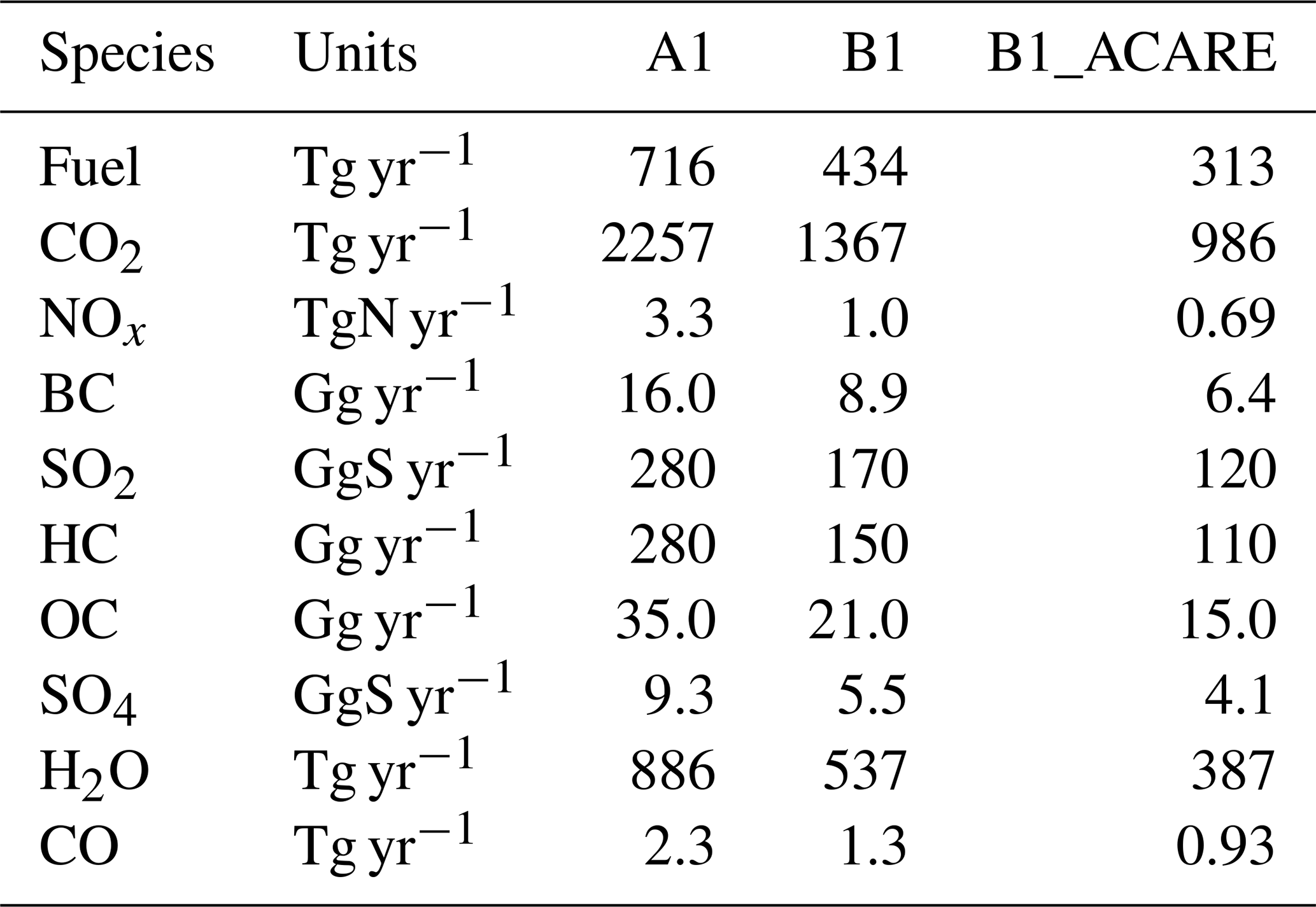
In this study, the future aircraft emission inventories prepared during the QUANTIFY EU project, and representative of the year 2050, are used (Owen et al., 2010). These scenarios were developed more than 10 years ago based on earlier economic assumptions regarding future Gross Domestic Product (GDP) growth and aviation demands in various regions according to the storylines of the former Intergovernmental Panel on Climate Change (IPCC) Special Report on Emission Scenarios (SRES) (Nakicenovic and Swart, 2000). They are still used in this study since they can be considered as benchmark scenarios, used in numerous former model simulations and intercomparisons (e.g. Koffi et al., 2010; Hodnebrog et al., 2011, 2012; Righi et al., 2016). These scenarios compare fairly well to the more recent inventories in terms of total future aircraft emissions. Three different aircraft emission inventories are selected in this study: the A1B (labelled QUANTIFY_A1 in the following discussion), B1 (QUANTIFY_B1), and B1_ACARE (QUANTIFY_B1_ACARE) scenarios. These are described in detail in Owen et al. (2010) and are only briefly summarized in the following discussion. The scenario A1B is representative of an intense growth of the aviation sector during the first part of the century, where global demand is driven by growth of the global economy. Due to technological improvements and the introduction of new and less polluting aeroplanes within the overall fleet, the fuel efficiency improvement is assumed to be approximately 1 % yr−1 over the period 2000–2050. In contrast, scenario B1 is a mitigation scenario in which the propensity to travel is reduced due to the goal of limiting the environmental impact of aviation and improving local air quality in particular. The fuel efficiency improves by 1 % yr−1 over the 2000–2020 period and increases by 1.3 % yr−1 after 2020. This leads to a significant reduction of NOx, SO2 and BC global emissions in 2050 for this scenario. Finally, assuming the technology targets of the Advisory Council for Aeronautical Research in Europe (ACARE) in 2010, the alternative scenario, B1_ACARE, is an ambitious mitigation scenario. Here the main goal is to limit the environmental impact of aviation. In this scenario, the fuel efficiency assumptions are further tightened and the efficiency improves by 2.1 % yr−1 after 2020. As a result, the fuel consumption is divided by more than a factor 2 compared to the A1B scenario in 2050. The reduction hypotheses behind this extreme goal are the ACARE 2050 goals, which, for example, aim at a 40 % improvement in aircraft fuel efficiency (with a further 10 % improvement from air traffic management) compared to an equivalent new aircraft introduced in 2000. The variables available from the QUANTIFY three-dimensional inventories are the fuel burn, NOx, and BC emissions. The highest NOx EIs derived from these inventories are for the A1B scenario and reaches 15.2 gNO2 kg−1 fuel (20 gNO2 kg−1 below 1800 m and 13.3 gNO2 kg−1 above 8400 m). For the mitigation scenarios B1 and B1_ACARE, the technology improvement strongly impacts the NOx emissions and the EIs decrease by about a factor of 2 (i.e. 7.9 gNO2 kg−1 fuel and 7.3 gNO2 kg−1 fuel for B1 and B1_ACARE, respectively). For BC, the EI remains fairly constant in the various QUANTIFY future scenarios (0.022, 0.021, and 0.019 gBC kg−1 fuel for A1B, B1, and B1_ACARE, respectively). The EIs for other species (i.e. H2O, CO, HC, OC, SO2, SO4) are assumed to be similar to those used for the REACT4C emission inventory.
In addition to the QUANTIFY A1, B1, and B1_ACARE scenarios, two other mitigation scenarios are used for the perturbation simulations. The QUANTIFY_LowNOx scenario is identical to the A1 scenario with the NO2 EI divided by a factor of 2. This scenario is intended to illustrate one of the ACARE objectives of reducing NOx emissions by the 2050 time-horizon compared to 2000. Similarly, the A1_Desulfurized scenario corresponds to the QUANTIFY_A1 scenario, with SO2 and sulfate emissions imposed to 0 to illustrate the impact of desulfurized fuels on the chemical composition perturbations and climate. Table 2 summarizes the total global emissions in 2050 for the different considered species and for the QUANTIFY_A1, QUANTIFY_B1 and QUANTIFY_B1_ACARE scenarios. As expected, for the QUANTIFY_A1 scenario, an increase in overall fuel consumption compared to the QUANTIFY_2000 of a factor of 3 is obtained and a factor 4 for NOx. For the QUANTIFY_B1 and QUANTIFY_B1_ACARE scenarios, the NOx emissions are reduced by a factor of 3.3 and 4.8, respectively, compared to the A1B scenario. The BC emissions are reduced by a factor of 1.8 and 2.5, respectively, and the SO2 emissions by a factor of 1.7 and 2.3 respectively. Figure S1 compares the zonal and annual mean distribution of REACT4C_2006 and QUANTIFY_A1_2050 fuel use, and NO2 and BC emissions.
Table 2Total global aircraft emissions for future 2050 baseline scenario QUANTIFY_A1 and for the two mitigation scenarios QUANTIFY_B1 and QUANTIFY_B1_ACARE.
For 2050, the total emissions from the QUANTIFY inventories are compared to the recent Shared Socioeconomic Pathways (SSP) scenarios (Hoesly et al., 2018) and the ACCRI AEDT scenarios (Brasseur et al., 2016) in Table S2. The ACCRI 2050-Base scenario is a high-emission scenario providing emissions even higher than the QUANTIFY_A1 scenario, particularly in terms of BC (81 % higher), SO2 (87 % higher), and to a lesser extent, NOx (20 % higher) emissions. We also note for comparison that Skowron et al. (2021) recently assumed a high air traffic growth and low technology development reaching a high NOx emission of 5.59 TgN yr−1 in 2050 in their “high scenario”, and a low air traffic growth and optimistic technology development reaching 2.17 TgN yr−1 in 2050 for the “low scenario”, intermediately between the A1B and B1 scenarios in terms of NOx emissions. The ACCRI 2050-S1 scenario also provides emissions intermediately between the A1B and B1 scenarios in terms of global NOx and BC emissions. Additionally, the SSP3-7.0 scenario, used as a reference in the AerChemMIP model intercomparison (Collins et al., 2017), provides NOx emissions intermediately between the QUANTIFY_A1 and QUANTIFY_B1 and BC and SO2 emissions close to QUANTIFY_A1. The mitigation scenario SSP1-2.6, also used as a mitigation option for the AerChemMIP simulations, is close to the QUANTIFY_B1_ACARE in terms of global emissions. This comparison suggests that the benchmark QUANTIFY scenarios used in this study are generally consistent with more recent aircraft scenarios in terms of global mean emissions and provide a reasonable estimate for both baseline and mitigation scenarios.
3.1 Model description
The LMDZ-INCA global chemistry–aerosol–climate model couples the LMDZ (Laboratoire de Météorologie Dynamique, version 6) general circulation model (GCM; Hourdin et al., 2020) and the INCA (INteraction with Chemistry and Aerosols, version 5) model (Hauglustaine et al., 2004, 2014) online. The interaction between the atmosphere and the land surface is ensured through the coupling of LMDZ with the ORCHIDEE (ORganizing Carbon and Hydrology In Dynamic Ecosystems, version 1.9) dynamical vegetation model (Krinner et al., 2005). In the present configuration, we use the “Standard Physics” parameterization of the GCM (Boucher et al., 2020). The model includes 39 hybrid vertical levels extending up to 70 km. The horizontal resolution is 1.9∘ in latitude and 3.75∘ in longitude. The primitive equations in the GCM are solved with a 3 min time step, large-scale transport of tracers is carried out every 15 min, and physical and chemical processes are calculated at a 30 min time interval. For a more detailed description and an extended evaluation of the GCM, we refer to Hourdin et al. (2020). The large-scale advection of tracers is calculated based on a monotonic finite-volume second-order scheme (Van Leer, 1977; Hourdin and Armengaud, 1999). Deep convection is parameterized according to the scheme of Emanuel (1991). The turbulent mixing in the planetary boundary layer is based on a local second-order closure formalism. The transport and mixing of tracers in the LMDZ GCM have been investigated and evaluated against observations for both inert tracers and radioactive tracers (e.g. Hourdin and Issartel, 2000; Hauglustaine et al., 2004), and in the framework of inverse modelling studies (e.g. Bousquet et al., 2011; Zhao et al., 2019).
The INCA model initially included a state-of-the-art CH4-NOx-CO-NMHC-O3 tropospheric photochemistry (Hauglustaine et al., 2004; Folberth et al., 2006). The tropospheric photochemistry and aerosol scheme used in this model version is described through a total of 123 tracers including 22 tracers to represent aerosols. The model includes 234 homogeneous chemical reactions, 43 photolytic reactions, and 30 heterogeneous reactions. Please refer to Hauglustaine et al. (2004) and Folberth et al. (2006) for the list of reactions included in the tropospheric chemistry scheme. The gas-phase version of the model has been extensively compared to observations in the lower stratosphere and upper troposphere. For aerosols, the INCA model simulates the distribution of aerosols with anthropogenic sources such as sulfates, nitrates, BC, OC, as well as natural aerosols such as sea salt and dust. The heterogeneous reactions on both natural and anthropogenic tropospheric aerosols are included in the model (Bauer et al., 2004; Hauglustaine et al., 2004, 2014). The aerosol model keeps track of both the number and the mass of aerosols using a modal approach to treat the size distribution, which is described by a superposition of five log-normal modes (Schulz, 2007), each with a fixed spread. To treat the optically relevant aerosol-size diversity, particle modes exist for three ranges: sub-micronic (diameter <1 µm) corresponding to the accumulation mode, micronic (diameter between 1 and 10 µm) corresponding to coarse particles, and super-micronic or super coarse particles (diameter >10 µm). This treatment in modes is computationally much more efficient compared to a bin scheme (Schulz et al., 1998). Furthermore, to account for the diversity in chemical composition, hygroscopicity, and mixing state, we distinguish between soluble and insoluble modes. In both sub-micron and micron size, soluble and insoluble aerosols are treated separately. Sea salt, SO4, NO3, and methane sulfonic acid (MSA) are treated as soluble components of the aerosol, dust is treated as insoluble, whereas BC and OC appear in both the soluble and insoluble fractions. The ageing of primary insoluble carbonaceous particles transfers insoluble aerosol number and mass to soluble with a half-life of 1.1 d. Ammonia and nitrate aerosols are considered as described by Hauglustaine et al. (2014). The aerosol component of the LMDZ-INCA model has been extensively evaluated during the various phases of AEROCOM (e.g. Gliß et al., 2021; Bian et al., 2017).
Earlier versions of the LMDZ-INCA model only including gas-phase tropospheric chemistry were used previously to assess the impact of subsonic aircraft on tropospheric ozone (Koffi et al., 2010; Hauglustaine and Koffi, 2012). These previous versions of the LMDZ-INCA model prescribed the ozone distribution to satellite observations above a potential temperature of 380 K, providing a strong constraint on the ozone perturbation at aircraft flight altitudes. In order to assess the impact of aircraft emissions on atmospheric composition, the model has been extended to include an interactive chemistry in the stratosphere and mesosphere. Chemical species and reactions specific to the middle atmosphere have been included. A total of 31 species were added to the standard chemical scheme, mostly belonging to the chlorine and bromine chemistry, along with 66 gas-phase reactions and 26 photolytic reactions. Water vapour is now affected by both physical processes in LMDZ and, in the stratosphere, an additional H2O tracer is introduced in INCA to account for photochemical production and destruction. In addition, heterogeneous processes on polar stratospheric clouds (PSCs) and stratospheric aerosols are parameterized in INCA following the scheme implemented in Lefèvre et al. (1994). The PSCs are first predicted as a function of the local partial pressures of H2O and HNO3, using the saturation vapour pressures for type I PSC (nitric acid trihydrate crystals) and for type II PSC (water ice) (Hanson et al., 1988; Carslaw et al., 1995). The excess of H2O and HNO3 is removed from the gas phase when saturation occurs and is used to compute the surface area concentration in the PSC region. Heterogeneous reaction rates are calculated explicitly, as a function of the surface area available, mean molecular velocity, and the reaction probabilities. Furthermore, the PSC scheme includes sedimentation of the cloud material. The fallout of PSC particles affects the vertical distribution of H2O, HNO3, and HCl. Condensed species are returned to the gas phase when clouds evaporate. In the presence of PSCs, the heterogeneous reactions convert bromine and chlorine reservoirs (HCl, HBr, ClONO2, BrONO2) into reactive species (Cl2, ClNO2, HOCl, Br2, BrNO2, HOBr) based on nine additional heterogeneous reactions introduced in the chemical scheme. The distribution of stratospheric aerosols is prescribed according to the Chemistry-Climate Model Initiative (CCMI) exercise (Thomason et al., 2018).
3.2 Model evaluation
We mostly refer to previous publications for a general evaluation of the LMDZ-INCA model performances and comparison against observations for both gas-phase chemistry and aerosols (e.g. Brunner et al., 2003, 2005; Hauglustaine et al., 2004; Folberth et al., 2006; Myhre et al., 2013; Hauglustaine et al., 2014; Koffi et al., 2016). The version of the LMDZ-INCA model used in this study and extended to the stratosphere has been evaluated by comparing model outputs with observations, particularly in the upper troposphere and lower stratosphere, before the model has been applied to investigate the impact of aircraft emissions. In this study, we summarize this evaluation for two key observational datasets.
Figure 1 summarizes the assessment of the modelled ozone seasonal cycle against ozonesondes as compiled by Tilmes et al. (2012) and with respect to the latitude and pressure domains. We present Taylor diagrams to summarize the model biases and correlations with the dataset. The model results are interpolated on both the horizontal and vertical to mimic the 42 ozonesonde station observations over the 1995–2011 observational period. The pressure levels are further grouped into pressure ranges represented by different colours for the sake of clarity. In terms of yearly mean biases, we distinguish two distribution modes for the three geographical domains, although it is less visible in the tropics (0–30∘): the 100–200 hPa pressure range (corresponding to the lower stratosphere in the middle (30–60∘) and high (60–90∘) latitudes), and the other pressure intervals throughout the troposphere. On the one hand, the 200–1000 hPa mean values show a tendency towards negative biases, especially at high latitudes where the modelled yearly averages spread from about 60 % to 100 % with respect to the observations, contrasting with the 80 % to 110 % interval elsewhere. On the other hand, most of 100–200 hPa yearly mean values are positively biased. In the middle and high latitudes, almost all the significant positive biases concern this pressure domain.
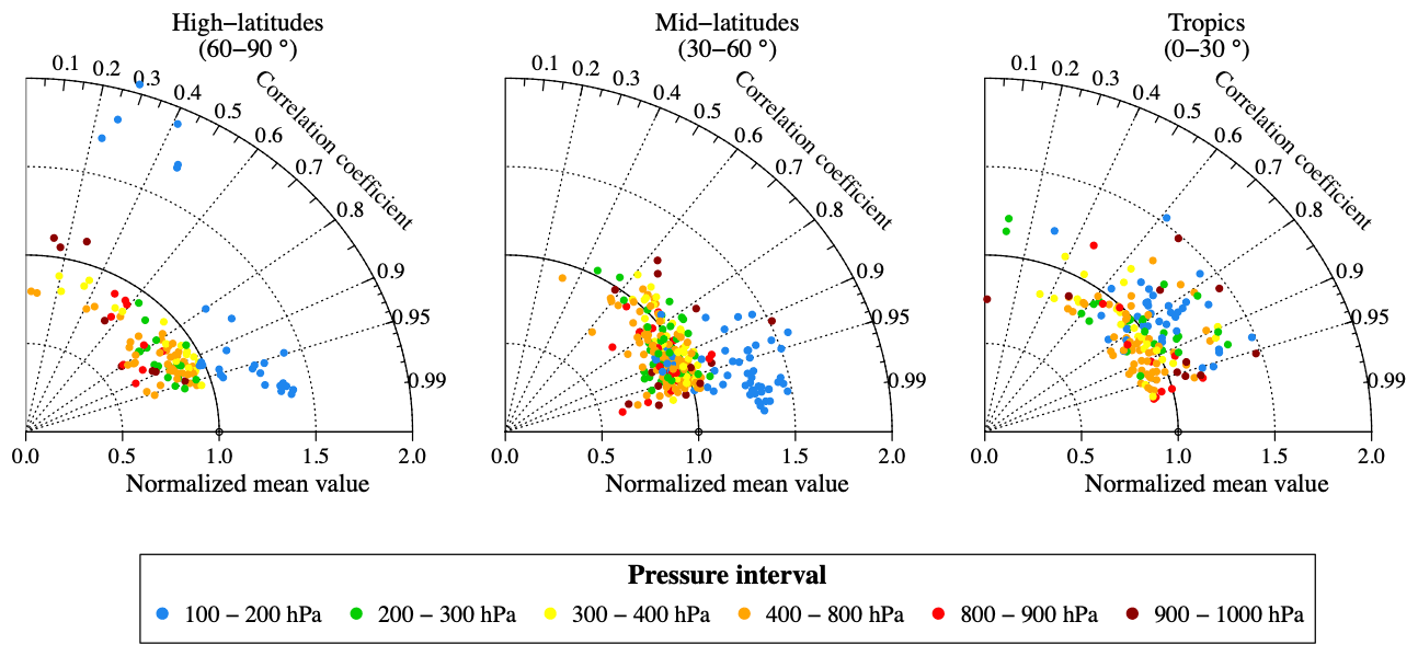
Figure 1Taylor diagram comparing the mean and temporal correlation of ozone volume mixing ratio between ozonesonde climatology over the 1995–2011 period (Tilmes et al., 2012) and LMDZ-INCA model results, interpolated to the sample locations and vertical levels for high latitudes (60–90∘), mid-latitudes (30–60∘) and tropical (0–30∘) stations. The colours correspond to different pressure ranges, each including different pressure levels (100–200 hPa: 3 levels; 200–300 hPa: 2 levels; 300–400 hPa: 2 levels; 400–800 hPa: 5 levels; 800–900 hPa: 2 levels; 900–1000 hPa: 2 levels).
With regards to correlation between observed and modelled seasonal cycles, Pearson's r coefficient mainly spreads from 0.60 up to 0.95, and is mostly greater than 0.8. Outside the tropics, this metric also shows distinct distribution modes between the same pressure domains. Higher correlations are reported in the 100–200 hPa interval where most r values are greater than 0.9 and part of them even reach the 0.99 value. Note that the six high-latitude points showing a poor correlation and a strong positive bias correspond to the three stations located in the southern polar region (Marambio, 64∘ S; Syowa, 69∘ S; Neumayer, 70∘ S) at 125 and 150 hPa. Consequently, although the simulation tends to overestimate lower-stratospheric ozone in the middle and high latitudes, it reproduces the seasonality particularly well outside the southern pole.
As with the Taylor diagrams, Fig. 2 provides the assessment of the modelled geographical distribution against IAGOS observations for ozone and CO, averaged over the periods December 1994–November 2017 and December 2001–November 2017, respectively (Cohen et al., 2018). The IAGOS (https://www.iagos.org/, last access: 7 September 2022) is a European research infrastructure performing in situ measurements on board several passenger aircraft (Petzold et al., 2015). Amongst the observed variables, ozone and CO have been monitored since August 1994 and December 2001, respectively. Information on the instruments is available in Thouret et al. (1998) and Marenco et al. (1998) for ozone and in Nédélec et al. (2003, 2015) for CO. The model assessment against the aircraft-based measurements is performed using the Interpol-IAGOS software (Cohen et al., 2021) that entails projecting the IAGOS data onto the model grid and deriving monthly means for each sampled grid cell. The model monthly averages are then derived from the daily output by applying a mask with respect to the IAGOS sampling. Lastly, for each dataset, these monthly outputs are used to derive seasonal and annual climatologies. For this comparison we apply the methodology for comparison with the global model described in Cohen et al. (2021). Since all four cruise-altitude levels are regularly crossed by the tropopause, each of them will contain both high-ozone (low-CO) and low-ozone (high-CO) grid cells. To account for these discrepancies while deriving a mean bias, thus to avoid absolute biases in high values to govern the results, the normalized mean value shown in these graphics is derived from the modified normalized mean bias (MNMB).
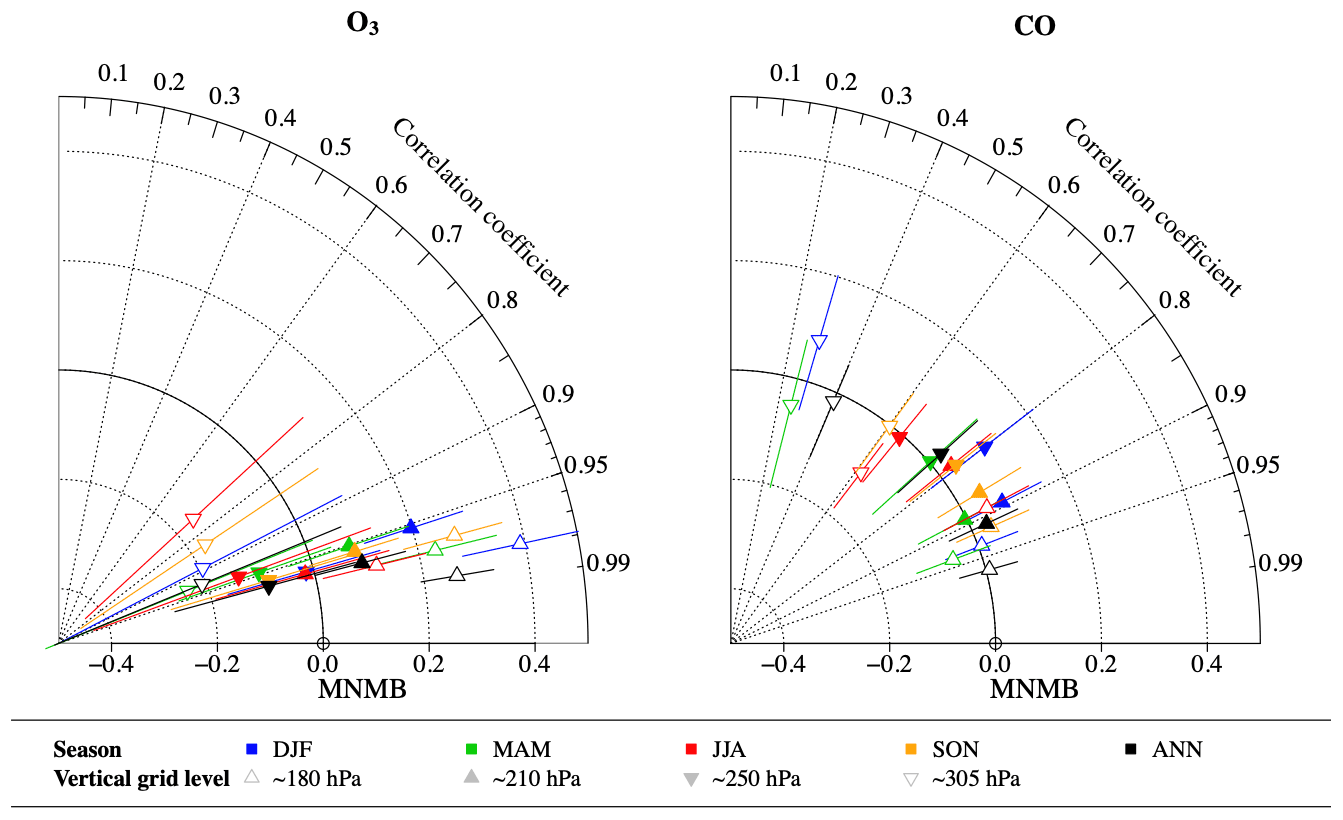
Figure 2Taylor diagram comparing the mean and geographical correlation of the volume mixing ratio of ozone (left) and carbon monoxide (right) between the IAGOS database (Cohen et al., 2018, 2021) and the LMDZ-INCA model results. The error bars denote the first and third quartiles of the model to IAGOS biases for a given vertical level and season.
In yearly means, the normalized mean value for ozone spreads from about 70 % up to 125 % and increases with the altitude, consistently with Fig. 1. It is also the case with the dependence on the season, represented by a 10 % difference at 300 hPa and a 30 % difference at 180 hPa. The same scheme is reproduced between the three highest levels, i.e. a lower summertime value and a greater wintertime value, likely depending on the distance from the tropopause. It suggests that the vertical ozone gradient in the lower stratosphere is overestimated by the model. However, the ozone geographical distribution is remarkably well correlated between the simulation and the observations, with all the yearly r coefficients greater than 0.92. This is especially the case at the highest levels. One possible reason is a good representation of tropopause motions at northern mid-latitudes, which ensures a realistic proportion between stratospheric and tropospheric air masses in most grid cells. Carbon monoxide is characterized by relatively small biases at the IAGOS-coverage scale, showing a balance between regional positive and negative biases. As for ozone, the correlation increases with altitude. However, the poor correlation reported at the lowest level highlights the difficulties to simulate the upward transport of pollutants in the troposphere.
The distribution of aerosol surface concentrations (sulfates, nitrates, ammonium) calculated with this version of the model has been evaluated and compared to surface stations by Hauglustaine et al. (2014) over Europe and Northern America and by Li et al. (2016) over China; it is not repeated here. However, Fig. S2 compares the calculated total aerosol optical depth (AOD) at 550 nm to the AERONET and MODIS observations for Eastern and Central China, Western Europe and the Eastern United States. A very good agreement is obtained for MODIS data with biases of −10 %, 1.4 %, and −6.1 % for these three regions, respectively, and a correlation coefficient r of 0.59, 0.55, and 0.86. Larger biases are calculated against AERONET data, particularly over regions characterized with very high aerosol loading such as China. Biases of respectively −39 %, 10 %, and 24 % are obtained for the three regions with correlation coefficients of 0.5, 0.45, and 0.78.
3.3 Model setup
In this study, meteorological data from the European Centre for Medium-Range Weather Forecasts (ECMWF) ERA-Interim reanalysis were used. The relaxation of the GCM winds towards ECMWF meteorology is performed by applying a correction term at each time step to the GCM u and v wind components with a relaxation time of 2.5 h (Hourdin and Issartel, 2000; Hauglustaine et al., 2004). The ECMWF fields are provided every 6 h and interpolated onto the LMDZ grid. We focus this work on the impact of aircraft emissions on atmospheric composition, its future evolution, and its direct RF of climate. In order to isolate the impact of aircraft emissions, all snapshot simulations are performed under present-day climate conditions and run for a period of 10 years after a 2-year spin-up. Therefore, ECMWF meteorological data for 2000–2009 are used. The perturbations are averaged over the last 3 years of the simulations. The impact of climate change on aircraft perturbations is however an interesting topic to be investigated in future studies.
For the baseline simulations, the anthropogenic emissions compiled by Lamarque et al. (2010) are added to the natural fluxes used in the INCA model. The ORCHIDEE vegetation model was used to calculate the biogenic surface fluxes of isoprene, terpenes, acetone, and methanol as well as NO soil emissions offline as described by Lathière et al. (2005). The NH3 emissions from natural soils and ocean are taken from Bouwman et al. (1997). Natural emissions of dust and sea salt are computed using the 10 m wind components from the ECMWF reanalysis. For the future simulations (2050), the Representative Concentration Pathways (RCP) 6.0 anthropogenic and biomass burning emissions provided by Lamarque et al. (2011) are used. Natural emissions for both gaseous species and particles are kept to their present-day level. Lightning is an important source of NOx in the upper troposphere at aircraft cruise altitudes. The lightning NOx emissions are parameterized in the model based on convective cloud heights as described in Jourdain et al. (2001). Based on this parameterization, the total lightning NOx emissions for the baseline simulation is 5.5 TgN yr−1. The methane surface mixing ratio used for both chemistry simulations and RF calculations is fixed to 1769 and 1895 ppbv for the present-day (2006) and 2050 baseline simulations, respectively. For N2O, the surface mixing ratio is fixed to 323 and 355 ppbv for 2006 and 2050, respectively.
The impact of aviation emissions on atmospheric composition is calculated based on a 100 % perturbation methodology, comparing the results of the simulations with aircraft emissions to a reference simulation with zero aircraft emissions. As discussed by Søvde et al. (2014), in previous work, both 5 % perturbations (e.g. Hoor et al., 2009; Hodnebrog et al., 2012) and 100 % perturbations (e.g. Gauss et al., 2006; Søvde et al., 2014) were applied. Koffi et al. (2010) compared the two methodologies and found that the 100 % perturbation of transport emissions induces a 6 % higher transport-induced ozone burden perturbation in the case of aircraft emissions. As noted by Søvde et al. (2014), the small perturbation approach is more adapted when different transport modes, affected differently by non-linearities, are compared. The 100 % perturbation gives the overall effect of aircraft, without considering compensating effects from other emission sectors due to chemical non-linearity (Koffi et al., 2010; Søvde et al., 2014; Grewe et al., 2019). This non-linear chemistry mostly depends on the background of NOx and HCs, and increases with larger perturbations in NOx. In this study we only focus on aircraft emissions, in contrast to other studies which compared the impact of emissions from different transport modes (e.g. Hoor et al., 2009; Koffi et al., 2010; Hodnebrog et al., 2012). A sensitivity analysis (as we envisaged our simulations) aims at characterizing the concentration change resulting from a given emissions change (Clappier et al., 2017). On the other hand, source apportionment approaches aim to quantify contributions by attributing a fraction of the pollutant concentration to each emission source (e.g. tagged species approach) (Grewe et al., 2010, 2019; Clappier et al., 2017; Matthes et al., 2021). The two methods provide different results but also different information. The source apportionment accounts for non-linearities and is used to retrieve information on the source contribution to the concentration of one pollutant (e.g. contributions of different transport modes to ozone). Sensitivity or impact methods are used to determine the impact of abatement strategies. In this study, which only focuses on aircraft impact, we adopt the 100 % perturbation, keeping in mind that this may mask some mild non-linearities. Table 3 summarizes the simulations performed and analysed in this study.
3.4 Radiative forcing (RF) calculations
Several RFs associated with atmospheric composition changes due to aircraft emissions are computed online during the LMDZ-INCA simulations. This is the case for the various components of the direct aerosol forcing in particular. The radiative calculations in the GCM are based on an improved version of the ECMWF scheme developed by Fouquart and Bonnel (1980) in the solar part of the spectrum and by Morcrette (1991) in the thermal infrared. The short-wave spectrum is divided into two intervals: 0.25–0.68 and 0.68–4.00 µm. The model accounts for the diurnal cycle of solar radiation and allows fractional cloudiness to form in a grid box. These RFs are calculated as instantaneous, clear-sky and all-sky forcings at the surface and at the top of the atmosphere. In Sect. 6, the all-sky forcings at the top of the atmosphere will be presented for aerosols as was done for instance by Hauglustaine et al. (2014).
A different protocol is used for ozone and stratospheric water vapour. For these two species, the RFs at the tropopause are calculated with an offline version of the LMDZ GCM radiative transfer model described above. In this offline version, the forcings are calculated on a monthly mean basis using the temperature, water vapour, cloud distributions, optical properties, surface albedo, and ozone fields stored from the GCM simulations and read from pre-established history files. The fixed-dynamical heating approximation is then applied to the calculations with a thermal adjustment of the stratosphere. The radiative code iterates until the forcings at the top of the atmosphere converge with the forcings at the tropopause. The iterations are performed with a 1-day time step over 200 d. This offline radiative transfer model has already been used to calculate the tropospheric ozone RFs in Berntsen et al. (2005) and more recently, in Li et al. (2016).
As described in previous work (e.g. Fuglestvedt et al., 1999; Skowron et al., 2013), the decrease in methane mixing ratio due to aircraft NOx emissions and associated with enhanced oxidation by OH, is responsible for a long-term methane direct RF that we calculate at equilibrium based on the change in the methane photochemical lifetime, including the methane feedback on its own lifetime. According to this methodology, the steady-state methane mixing ratio decrease due to aircraft emissions is given by (Prather, 1994; Fiore et al., 2009; Holmes, 2018)
where is the new steady-state methane mixing ratio, is the reference methane mixing ratio (taken as 1769 ppbv for the present day and 1985 ppbv in 2050), f denotes the methane feedback on its own lifetime (Prather et al., 2001; Holmes et al., 2011), and (%) is the change in the methane lifetime due to aircraft emissions and subsequent OH perturbation. The associated direct RF of climate of this change in methane is calculated using the simple formula revised by Etminan et al. (2016). As reported by these authors, the inclusion of the short-wave contribution in this revised expression results, for instance, in a 24.5 % increase of the methane forcing associated with a halving of its concentration, compared to the previous literature (Myhre et al., 1998). For the methane feedback factor, f, Prather et al. (2001) derived a best estimate value of 1.4 based on a multimodel range of 1.33–1.45. A similar best estimate value was recommended by Holmes et al. (2011). Fiore et al. (2009) derived a multimodel ensemble mean of 1.33 and a range of 1.25–1.43, including a value of 1.31 contributed with an earlier version of the LMDZ-INCA model. The feedback factor has been recalculated in this study for the current version of our model based on a reference simulation and a 10 % perturbation in methane surface mixing ratio simulation. Based on this set of simulations and the methodology described in Fiore et al. (2009), we recalculated a methane feedback factor f of 1.36, in agreement with the previous estimates. This factor is then used in Eq. (1) in order to derive the change in methane mixing ratio due to aircraft emissions and the associated RF of climate. It should be noted that this estimate of the methane feedback is based on fixed surface CH4 concentrations. Other methodologies have also been proposed to evaluate this feedback and in particular, the use of methane surface fluxes (Khodayari et al., 2015; Pitari et al., 2016). Khodayari et al. (2015) concluded that for the simulations with fixed CH4 at the lower boundary condition, the parameterization based on Eq. (1) using the global mean lifetime approach overestimates the change in CH4 by 8.6 % compared to the change calculated directly from the model using CH4 surface emissions. The overestimation is 12.1 %–20.0 % if using other lifetime approaches. They concluded that the parameterization based on Eq. (1) is good within ∼10 % when using the global mean lifetime approach.
The indirect forcings associated with this change in methane mixing ratio through long-term tropospheric ozone and stratospheric water-vapour adjustments were recalculated with the LMDZ-INCA global model. This was done by imposing the new steady-state methane surface mixing ratio (1744 ppbv) calculated from Eq. (1) for the present-day REACT4C_2006 simulation in the three-dimensional model and running it for a period of 10 years in order to determine the associated change in ozone and stratospheric water vapour by comparing it to a reference simulation using (1769 ppbv) as methane surface mixing ratio. In this case, we calculated a change in ozone after 10 years of −0.93 Tg (0.085 DU) and a change in stratospheric water vapour of −2.12 Tg. Thereafter, we calculated ozone and stratospheric water vapour RFs for these perturbations. These calculations provide an indirect long-term ozone forcing of 116 mW m−2 ppmv−1 of CH4 and an indirect long-term stratospheric water vapour forcing of 27 mW m−2 ppmv−1 of CH4. The ozone forcing is smaller by 17 % compared to the value of 140±70 mW m−2 ppmv−1 provided by Forster et al. (2021), but well within the provided confidence level. For stratospheric H2O, the forcing is subject to a larger uncertainty, and we derive a lower forcing by 32 % compared to the value of 40±40 mW m−2 ppmv−1 provided by Forster et al. (2021), but also well within the confidence level. These calculated forcings were then used to derive the indirect long-term ozone and water vapour forcings for the other aircraft emission scenarios based on a simple scaling with the methane mixing ratio change calculated with Eq. (1) for all simulations.
Carbon dioxide is the end product of the methane atmospheric oxidation. Hence, the production of CO2 is an indirect RF resulting from the change in methane mixing ratio due to increased oxidation by OH from aviation NOx emissions. Since intermediate carbon containing methane oxidation products are subject to dry and wet deposition, not every oxidized methane molecule results in a produced CO2 molecule. In this study, we assume that 1 molec. of change in CH4 oxidation leads to 0.6 molec. of CO2 produced (Folberth et al., 2005; Boucher et al., 2009). The decrease in CH4 due to enhanced oxidation is then translated into a change in CO2 and converted to an RF based on the simple formula from Myhre et al. (1998). Based on the REACT4C_2006 change in methane mixing ratio, we derive an indirect CO2 forcing F of 8.25 mW m−2 ppmv−1 of CH4. This normalized number is used to calculate the forcings for the other simulations.
4.1 Aviation impact on atmospheric composition
Figure 3 presents the daily changes in concentration associated with the base REACT4C_2006 aircraft emission inventory for several key species at 250 hPa (i.e. cruise altitude). For NOx, a strong seasonal cycle is calculated with a fall–winter maximum reaching 39 pptv and a summer minimum of 15–20 pptv located at 30–60∘ N and corresponding mostly to the transatlantic flight corridors. A northward transport of NOx, associated with the transport of mid-latitude air masses to the polar regions is visible. During spring, the NOx mixing ratio increases by up to 20 pptv at high latitudes. The geographical distribution depicted in Fig. 4 shows that NOx increases by up to 60 pptv in regions with high aircraft emissions over Europe and North America. It also extends to Northeast Asia and Japan, reaching more than 40 pptv. As a consequence of this increase in NOx concentrations, ozone increases by 3–6 ppbv at flight altitude at northern mid-latitudes. A marked seasonal cycle (Fig. 3), associated with the NOx increase and higher photochemical activity, is calculated at mid–high northern latitudes and peaks in May. This maximum reached in May at high latitudes results from a combination of a more intense photochemical activity in summer combined with a more intense transport poleward in spring. As a consequence, the peak is reached at the end of the spring season. A maximum zonal mean ozone increase reaching almost 7 ppbv is calculated in polar regions where photochemistry is active and where mid-latitude ozone is transported and accumulates. Due to its longer lifetime, the change in ozone at 250 hPa reaches 2–4 ppbv over most of the Northern Hemisphere above 30∘ N (Fig. 4).
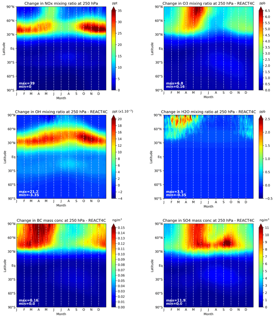
Figure 3Daily and zonally averaged perturbations due to aircraft emissions at 250 hPa of NOx (pptv), O3 (ppbv), OH (10−3 pptv), H2O (ppbv), BC (ng m−3), and SO4 (ng m−3) for the REACT4C_2006 inventory.
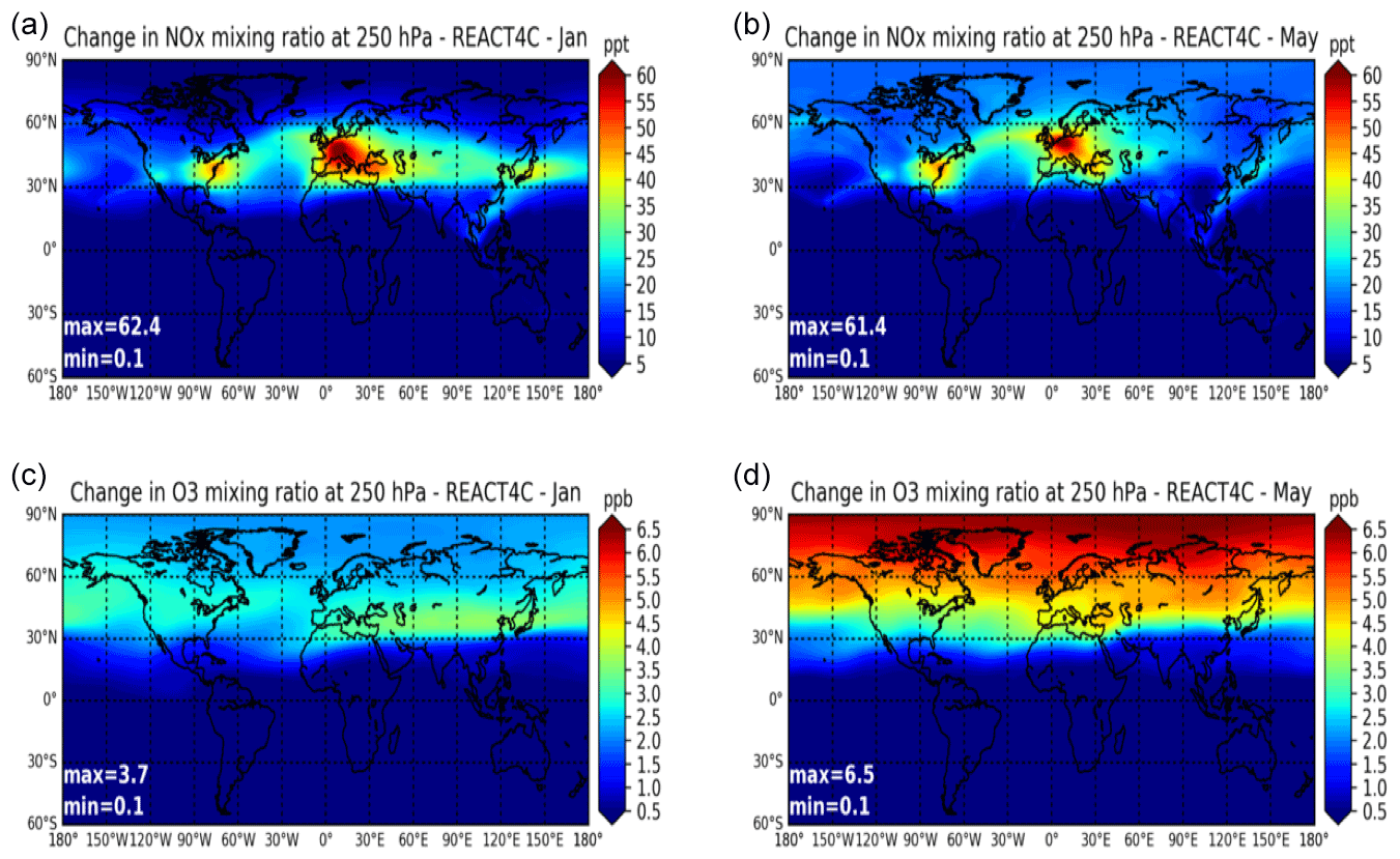
Figure 4Spatial distribution of the 250 hPa perturbations due to aircraft emissions for the month of January (a, c) and May (b, d) for the mixing ratios of NOx (pptv) and ozone (ppbv) for the REACT4C_2006 inventory.
The zonal mean distributions of the NOx and O3 perturbations are shown in Fig. 5 for January and May. These 2 months are chosen in order to illustrate the minimum and maximum perturbations in atmospheric composition. The NOx increase reaches a maximum of about 45 pptv (60 %) at 250 hPa and at 40–60∘ N during both seasons. In May, the mixing of air masses towards higher latitudes is visible with increased mixing ratios reaching about 25 pptv at the pole. The induced ozone perturbation ranges from a maximum of 3 ppbv in January to a maximum of 6–7 ppbv in May (4 %). These results agree with the model intercomparison of Søvde et al. (2014) who calculated, with the same aircraft emission inventory, a maximum ozone increase ranging from 4.8 to 8.8 ppbv during summer, and a lower impact in winter associated with less photochemical activity, and ranging from 3.4 to 4.4 ppbv. They are also in agreement in terms of distribution and ozone increase with the earlier model intercomparison results by Hoor et al. (2009) obtained with the QUANTIFY_2000 emission inventory, and with the peak absolute ozone increase of 5 to 8 ppbv calculated by Olsen et al. (2013). The calculated maximum ozone perturbation occurs between 300 and 200 hPa in both seasons. A downward transport of the ozone produced is visible down to 800 hPa at 30–40∘ N. Due to higher photochemical activity at high latitudes (>60∘ N), and mixing and accumulation of air masses around the pole, the ozone increase is centred in polar regions during May. In winter, this maximum is located at lower latitudes between 40 and 60∘ N, as illustrated in Fig. 4. The maximum perturbation associated with aircraft emissions appears just above the tropopause at high latitudes, showing the need to account for chemistry in both the troposphere and the stratosphere (Gauss et al., 2006; Søvde et al., 2014; Khodayari et al., 2014a). As a result of the NOx and hence ozone increases, an increase of OH located between 30 and 50∘ N, depending on the solar radiation seasonal cycle, and reaching pptv is calculated (Fig. 3).
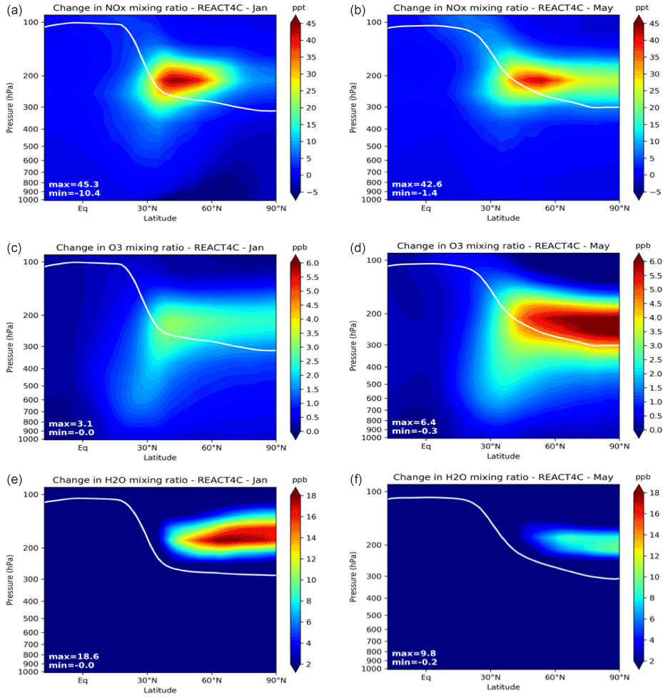
Figure 5Zonal mean perturbations due to aircraft emissions for January (a, c, e) and May (b, d, f) of NOx (pptv), O3 (ppbv), and H2O (ppbv) for the REACT4C_2006 inventory. The solid line represents the model tropopause pressure.
The increase in water vapour associated with H2O aircraft emissions shows a strong seasonal cycle and reaches a maximum of 3.5 ppbv in spring at 250 hPa (Fig. 3). The zonal mean distribution (Fig. 5) shows that the maximum is located in the stratosphere where the water vapour lifetime is longer. The increase in stratospheric water vapour reaches 19 ppbv (0.2 %) at 200 hPa in January at 60∘ N. In May, the increase reaches about 10 ppbv at this latitude. This is significantly lower than the 64 ppbv annual mean maximum increase calculated by Wilcox et al. (2012) with a Lagrangian model and considering water vapour as a passive tracer. With a Lagrangian model, Morris et al. (2003) also calculated an increase of water vapour due to aircraft emissions of more than 150 ppbv just above the tropopause and less than 2 ppbv in the stratosphere. In our model setup, the increase of water vapour is reset to zero below the model tropopause at each time step, strictly limiting the aircraft perturbation to a stratospheric perturbation.
For BC (Fig. 3), the seasonal cycle is well marked with a maximum reaching 0.16 ng m−3 in winter–spring and a minimum in summer of 0.01 ng m−3. This aerosol accumulates at cruise altitude during winter, leading to a marked maximum. In summer, due to more intense atmospheric mixing, these high concentrations are mixed to lower altitudes. Meridional and poleward transport is also visible for these particles and higher concentrations are reached from 40∘ N to the pole, in agreement with the transport of NOx discussed earlier. The change in SO2 concentration (not shown) exhibits a similar feature with a winter maximum reaching more than 6 pptv. For this aerosol precursor, despite direct aircraft emissions, a decrease is calculated in summer reaching 3.5 pptv, and corresponding to the SO2 oxidation by OH-forming sulfate particles. As a consequence of this enhanced production, a maximum increase in SO4 is calculated from May to September and reaches 8–12 ng m−3 (Fig. 3).
Figure 6 shows the geographical distribution of the BC perturbation at 250 hPa. In January, the maximum reaching 0.17 ng m−3 is located over source regions in North America, Europe, and Eastern Asia with zonal transport over the Pacific and Atlantic flight corridors. The distribution in May clearly shows transport and accumulation of BC in polar regions. The zonal mean distribution of the BC perturbation is shown in Fig. 7 and exhibits a maximum of 0.15 ng m−3 (1 %) between 300 and 200 hPa at 40–70∘ N. A redistribution of these flight altitude emissions through subsidence is visible with a secondary maximum of about 0.08 ng m−3 (0.15 %) calculated in the lower troposphere around 30∘ N. These results are in line with the perturbations calculated by Righi et al. (2016) and range from 0.05–0.1 ng m−3 in annual mean at cruise altitude in the Northern Hemisphere. In the lower troposphere, Righi et al. (2016) calculated a somewhat higher BC concentration increase, reaching up to 0.5 ng m−3 near the surface.

Figure 6Spatial distributions of the 250 hPa perturbations due to aircraft emissions for January (a, c, e) and May (b, d, f) for BC, SO4, and NO3 (ng m−3) for the REACT4C_2006 inventory.
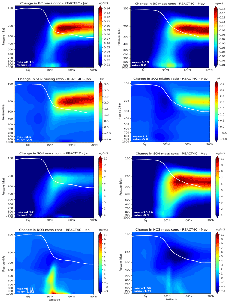
Figure 7Zonal mean perturbations due to aircraft emissions for January (left) and May (right) of BC (ng m−3), SO2 (pptv), SO4 (ng m−3), and NO3 (ng m−3) for the REACT4C_2006 inventory. The solid line represents the tropopause pressure.
The geographical distribution of sulfates at 250 hPa (Fig. 6), clearly shows a strong seasonal cycle associated with increased oxidation of SO2 in spring, reaching 14 µg m−3 in May over a large part of Europe and Asia. In Fig. 7, the zonal mean SO2 perturbation varies between 8 ppt (40 %) in January and 5 ppt (30 %) in May at 200 hPa between 40 and 90∘ N. The associated sulfate perturbation reaches a maximum of 10 ng m−3 (4 %) in May with a minimum of 5 ng m−3 (3 %) simulated in January and localized, as for BC, between 300 and 200 hPa at the latitude band between 30–50∘ N and with a clear poleward transport in May. As seen for BC, a significant subsidence of the sulfate perturbation is calculated between 30–40∘ N. Again, these results agree with the perturbations calculated by Righi et al. (2016) with the EMAC model, reaching 2–5 ng m−3 in annual mean at cruise altitude in the Northern Hemisphere. In the lower troposphere, Righi et al. (2016) calculated a higher SO4 concentration increase reaching up to 10 ng m−3 near the surface. Since similar EIs are used in both studies, this points towards a more efficient removal of aerosols in LMDZ-INCA than in EMAC.
Nitrates are not emitted by aviation, but their distribution is affected by two competing processes. On the one hand, the increase of SO4 reduces the amount of NH3 available for ammonium nitrate formation, and on the other hand, the increase of NOx enhances the production of nitrates. At cruise altitudes, the strong increase in SO4 dominates and an overall decrease in nitrates of up to −7 µg m−3 (7 %) is calculated in May over Europe and Asia, collocated with the increase in sulfates (Fig. 6). In regions characterized by high NH3 concentrations, in India or Southeast Asia, enough ammonia is still present after ammonium sulfate production to increase the production of ammonium nitrate when more NOx associated with aircraft emissions are present. This is the case, particularly in January around 30∘ N in the lower troposphere (Fig. 7), but also at cruise altitudes in localized areas in India and Southeast Asia (Fig. 6). In these regions, an increase of nitrates reaching more than 9 ng m−3 is calculated. Righi et al. (2016) calculated a very similar zonal mean pattern for the nitrate concentration perturbation, decreasing in the upper troposphere by up to 1 µg m−3 in annual mean and increasing by 5–10 ng m−3 in the lower troposphere. Similarly, the zonal mean perturbation pattern for nitrate aerosols agrees with the results presented by Unger (2011).
4.2 Impact of flight altitude changes
The atmospheric lifetime of pollutants emitted by aviation is highly dependent on the altitude at which they are injected into the atmosphere (Grewe et al., 2002; Gauss et al., 2006; Frömming et al., 2012; Søvde et al., 2014; Matthes et al., 2017). The sensitivity of the calculated perturbations to the flight altitude is illustrated in this section based on the REACT4C_PLUS and REACT4C_MINUS emissions, respectively corresponding to an increase or decrease of the flight cruise altitude at 2000 ft compared to the REACT4C_2006 baseline inventory.
Figure 8 shows the impact of the flight altitude variation on the zonal mean distribution of key species compared to the baseline scenario. These variations are illustrated for May conditions when the maximum impact of aircraft emissions is calculated by the model, as illustrated in the previous section. As a consequence of the chemical lifetime increase with altitude, a higher (resp. lower) flight cruise altitude increases (resp. decreases) the change in ozone mixing ratio by 1.7 ppbv (30 %) (resp. −1.6 ppbv) between 150 and 250 hPa compared to the baseline scenario. The impact on ozone is comparable to the results obtained by Søvde et al. (2014) and Matthes et al. (2017, 2021) (1–2 ppb in summer and 0.4–1 ppb in winter). Similarly, the BC concentration increases by 0.031 ng m−3 (20 %) when the flight altitude is increased and, in contrast, decreases by 0.032 ng m−3 with a lowered flight altitude.
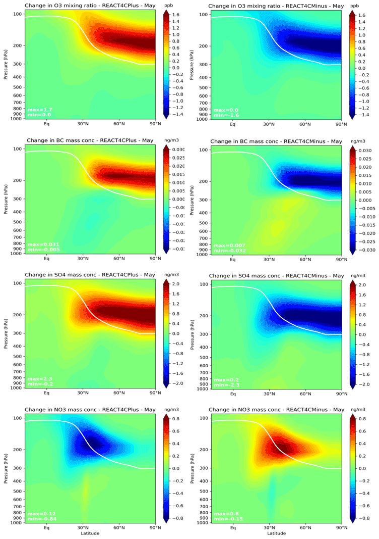
Figure 8Zonal mean difference for the months of May for O3 (ppbv), BC (ng m−3), SO4 (ng m−3), and NO3 (ng m−3) between the REACT4C_PLUS (left) and REACT4C_MINUS (right) simulations and REACT4C_2006 as the reference. The solid line represents the tropopause pressure.
Directly related to the response of SO2 to flight altitude changes, the concentration of sulfates shows a behaviour similar to the primary aerosol BC, and increases by a maximum of 2.3 ng m−3 (22 %) between 250 and 150 hPa at 40–90∘ N in the REACT4C_PLUS simulation and decreases by 2.3 ng m−3 in the REACT4C_MINUS simulation. In contrast, the variation of nitrate aerosols shows an opposite behaviour associated with the change in sulfates. An increase in sulfates reduces the NH3 available for forming ammonium nitrate particles in favour of ammonium sulfates, and NO3 decreases by 0.84 ng m−3 (23 %) at flight altitude in the REACT4C_PLUS simulation. Please note that the change in sulfates is maximum at high latitudes but the maximum perturbation in nitrates occurs at lower latitudes (around 30∘ N) where more NH3 is present at this altitude. Similarly, the decrease in sulfate concentration calculated in the REACT4C_MINUS scenario induces an increase of ammonium nitrate particles of 0.83 ng m−3 at 200 hPa. These sensitivity simulations show that changing the aircraft flight altitude has a marked impact on the ozone and aerosol responses to emissions (of about 20 %–30 % compared to the baseline simulation in May), and hence on the associated RFs, as will be analysed in the Sect. 6.
5.1 Future baseline scenario
In addition to these simulations using the REACT4C_2006 emission inventory, a set of future simulations using the QUANTIFY emission inventories has been conducted for the year 2050. The corresponding distributions of the baseline perturbations for the QUANTIFY_2000 inventory are in line with the results obtained for REACT4C_2006 (Fig. S3). However, in the case of the QUANTIFY_2000 emissions, particularly due to the higher fuel consumption, the maximum perturbations are generally slightly higher. In the zonal mean, these perturbations reach 6.8 ppbv for ozone in May, between 250 and 350 hPa, 0.16 ng m−3 for BC, 11.3 ng m−3 for SO4, and −3.95 ng m−3 for NO3, to be compared with 6.4 ppbv, 0.15, 10.2, and −3.71 ng m−3, respectively, in the case of REACT4C_2006 (see Sect. 4).
For future simulations (2050), the baseline simulation corresponds to the aviation emissions from the QUANTIFY_A1 inventory. Figure 9 illustrates the perturbation associated with aircraft emissions for this scenario for key constituents (May as the seasonal maximum of the perturbation). The NOx mixing ratio increases in the upper troposphere by up to 194 pptv in January at 200 hPa and 170 pptv (250 %) in May (not shown). As a consequence, ozone increases from 9.2 ppbv in January to up to 19.6 ppbv (15 %) in May at flight altitude. These values are comparable to the values calculated by Søvde et al. (2007) (7 to 18 ppbv for monthly averages in January and May, respectively) but higher than the ozone increase calculated by Koffi et al. (2010) (10 ppbv in July) and the model mean given by Hodnebrog et al. (2012) for the same emission inventory. We note however that only a few models used in Hodnebrog et al. (2012) included an interactive chemistry in the stratosphere, thereby imposing ozone to climatologies or calculated with simplified parameterizations in this region. This could consequently dampen the response of ozone in the upper troposphere. This finding is confirmed by the higher tropospheric ozone increase associated with aircraft NOx emissions calculated by global models, including interactive chemistry in both the troposphere and the stratosphere (Olsen et al., 2013; Khodayari et al., 2014a; Brasseur et al., 2016; Skowron et al., 2021). The increase in BC is also significant and reaches 0.6 ng m−3 in January and 0.55 ng m−3 (5 %) in May, a factor of 3 larger than the QUANTIFY_2000 perturbation. As noted earlier, in addition to the maximum increase at flight altitude, a secondary maximum reaching 0.3 ng m−3 and associated with the downward redistribution of aircraft emissions is also calculated at ground level. The increase in SO4 for this scenario reaches 15.6 ng m−3 in January and 32.8 ng m−3 (15 %) in May. The marked increase in SO4 concentrations at cruise altitude is responsible for a subsequent decrease in NO3 reaching −9.4 and −21 ng m−3 in May (50 %). Below about 500 hPa, an increase in NO3 concentrations reaching 14 ng m−3 (10 %) in May and as much as 47 ng m−3 (5 %) in January is simulated. These increased surface concentrations in 2050 are mostly associated with much higher NH3 background concentrations at the surface in the future (particularly in Southeast Asia) (Hauglustaine et al., 2014), and subsequent enhanced NO3 formation due to redistribution of aircraft NOx emissions to lower levels forming ammonium nitrates. This result agrees with the findings of Righi et al. (2016) and Unger (2011), who calculated a decrease of nitrate particles in the NH3-limited mid-upper troposphere due to aircraft emissions as well as an increase in the lower troposphere and at surface. This is however in contrast with the results of Unger et al. (2013), who calculated an increase of NO3 associated with aircraft emissions in most of the troposphere, with a moderate 2 %–3 % decrease in the upper troposphere and lower stratosphere, and consequently derived a strong negative forcing by nitrate particles as also reported by Brasseur et al. (2016). Please note that the impact of future climate change on aircraft perturbations is not considered in our simulations and should be investigated in forthcoming studies.
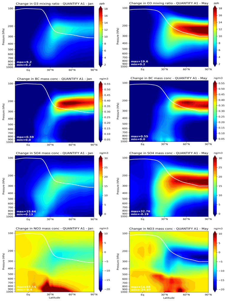
Figure 9Zonal mean perturbations due to aircraft emissions for the months of January (left) and May (right) for O3 (ppbv), BC (ng m−3), SO4 (ng m−3), and NO3 (ng m−3), averaged for the future scenario QUANTIFY A1 2050. The solid line represents the tropopause pressure.
5.2 Mitigation scenarios
Two alternative future scenarios are derived from the future scenario QUANTIFY_A1. As described in Sect. 2, the QUANTIFY_LowNOx scenario simulates the impact of NOx emissions reduced by a factor of 2, mimicking a significant improvement of the engine combustion technology with respect to the NOx EI. The QUANTIFY_A1_Desulfurized scenario simulates the impact of a desulfurized fuel. In addition, two alternative scenarios representing two aircraft emission mitigation trajectories are used, i.e. the QUANTIFY_B1 and QUANTIFY_B1_ACARE scenarios described by Owen et al. (2010) and summarized in Sect. 2.
Figure 10 shows the impact of the LowNOx and Desulfurized future emission scenarios on the zonal mean distribution of key atmospheric species. The low NOx emissions have a significant impact on the ozone increase. In this case, the zonal mean ozone increase reaches a maximum of 5.9 ppbv in January (not shown) and 12 ppbv (8 %) in May at 200 hPa. This corresponds to a reduction of 3 ppbv in January and 7 ppbv (40 %) in May compared to the QUANTIFY_A1 scenario (Fig. 9). In this scenario, SO4 is only moderately affected at flight altitude and the maximum SO4 increase in May remains close to 33 ng m−3(15 %). However, in the lower troposphere, less sulfates are produced in the aqueous phase at lower O3 concentrations, especially in subsidence regions. The increase in SO4 at the surface is significantly reduced and decreases from about 17 ng m−3 at 30∘ N in the QUANTIFY_A1 scenario to less than 10 ng m−3 in the QUANTIFY_LowNOx simulation. Moreover, as shown in Fig. 10, the impact on NO3 is very limited at the flight cruise altitude. However, in the lower troposphere, the formation of nitrates through the reaction with NH3 is decreased at lower NOx emissions and the increased NO3 concentration at the surface reaches 7 ng m−3 to be compared with the 14 ng m−3 calculated in the QUANTIFY_A1 simulation (Fig. 9). This is a reduction factor of 2, linear with the decrease in total NOx aircraft emissions in this scenario. This LowNOx scenario has a significant impact on air quality, reducing not only tropospheric ozone but also the concentration of sulfates and nitrates in the lower troposphere.

Figure 10Zonal mean perturbations due to aircraft emissions for May of O3 (ppbv), SO4, and NO3 (ng m−3) for the LowNOx (a, c, e) and Desulfurized (b, d, f) scenarios. The solid line represents the tropopause pressure.
In comparison to the QUANTIFY_A1 baseline scenario, the QUANTIFY_A1_Desulfurized simulation has, as expected, a significant impact on the SO2 aircraft perturbation, and consequently on the formation of SO4. As seen from Fig. 10, since no emission of SO2 and SO4 are considered in this simulation, the SO4 increase reaching 13 ng m−3 (5 %) in May around 30∘ N and at 300–200 hPa is only associated with the increased production from SO2 oxidation at higher ozone and OH concentrations. As a consequence of the reduced change in SO4, a very moderate decrease in nitrates reaching only −6 ng m−3 (5 %) is calculated at flight altitude. In the lower troposphere, the increase in NO3 associated with the production of ammonium nitrate from surface NH3 emissions and aircraft NOx reaches 14 ng m−3 (10 %), as also calculated in the QUANTIFY_A1_Desulfurized scenario. These results agree with Unger (2011) and Kapadia et al. (2016), who calculated a similar impact of desulfurized fuel, a much lower increase of sulfates and nitrates at flight altitude, and a significant increase in nitrates in the lower troposphere. As in Unger (2011), but in contrast with earlier work by Pitari et al. (2002), little effect of sulfate aerosols on ozone via heterogeneous chemistry is predicted in the upper troposphere. The impact of aircraft desulfurized fuel is close to the regular fuel ozone perturbation.
The results for the alternative economic and technological scenarios, QUANTIFY_B1 and QUANTIFY_B1_ACARE (Owen et al., 2010), are illustrated in Fig. 11. A primary objective of the QUANTIFY_B1 mitigation scenario is to improve air quality; therefore the reduction of NOx, SO2, and BC emissions are relatively important compared to the baseline future scenario QUANTIFY_A1. In this case, as a consequence of lower NOx emissions, the O3 perturbation is reduced by more than a factor of 2 compared to QUANTIFY_A1, and the ozone zonal mean increase reaches a maximum of 4.5 ppbv in January (not shown) and 8.6 ppbv (6 %) in May compared to 9.2 and 19.6 ppbv in January and May, respectively, for the QUANTIFY_A1 simulation. For this mitigation scenario, Hodnebrog et al. (2011) derived a model mean ozone increase at cruise altitude of 3 ppbv in January and about 5 ppbv in July, somewhat lower than our results. Again, it should be noted that none of the models used in Hodnebrog et al. (2012) included an interactive chemistry in the stratosphere. The BC perturbation reaches a maximum of 0.35 ng m−3 (3 %) at flight altitude, to be compared with 0.55 ng m−3 in the QUANTIFY_A1 simulation. The sulfate concentrations increase in May by up to 22 ng m−3 (9 %), and consequently, SO4 increase and NO3 are reduced by −14 ng m−3 (40 %) at flight altitude, compared to 33 and −22 ng m−3, respectively, for the QUANTIFY_A1 scenario. The alternative scenario, QUANTIFY_B1_ACARE, is the most ambitious mitigation future scenario used in this study, with very strong emission reductions. This scenario is an “extreme” scenario to limit the environmental impact of aviation. In this scenario, the NOx emissions are reduced by almost a factor of 5 and the ozone increase reaches a maximum of 6.2 ppbv (4 %) in May, a value even lower than the ozone increase calculated under the QUANTIFY_2000 (6.8 ppbv) and REACT4C_2006 (6.4 ppbv) simulations. A significantly attenuated aerosol increase is also calculated for the QUANTIFY_B1_ACARE scenario, and BC and SO4 increase by up to 0.25 ng m−3 (2 %) and 16 ng m−3 (7 %) at flight altitude, respectively. The nitrate concentration decreases by 10 ng m−3 (30 %) at flight altitude and increases by up to 3.8 ng m−3 (3 %) in the lower troposphere (Fig. 11).
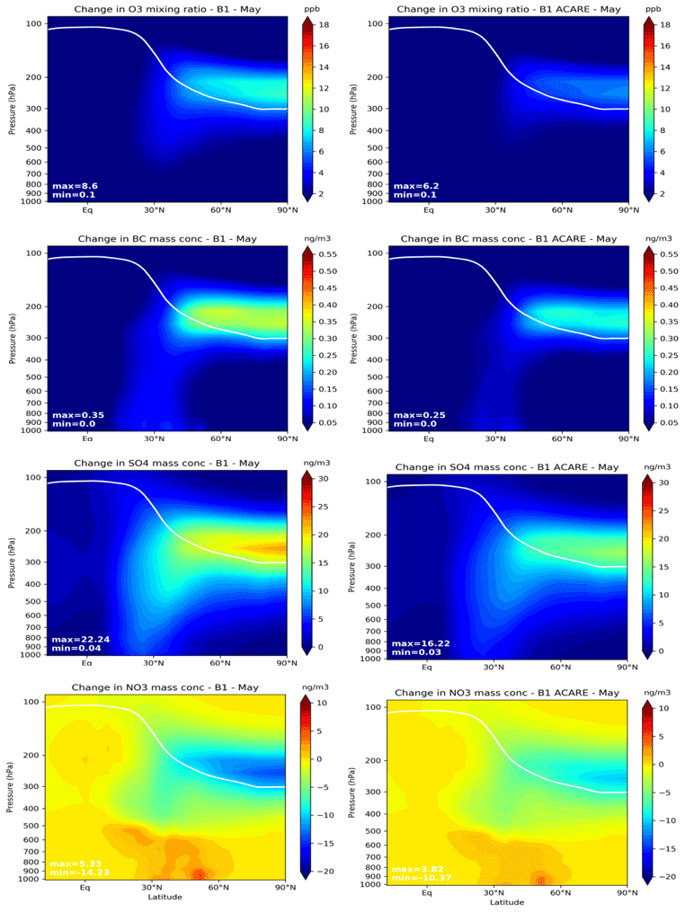
Figure 11Zonal mean perturbations due to aircraft emissions for May of O3 (ppbv), BC, SO4, and NO3 (ng m−3) for the QUANTIFY 2050 B1 (left) and B1 ACARE (right) scenarios. The solid line represents the tropopause pressure.
6.1 Changes in ozone burden and methane lifetime
Table 4 summarizes the impact of aircraft emissions on the global burden of ozone and methane lifetime. Ozone increases by 4.7 Tg (0.430 DU) for the REACT4C_2006 reference scenario and an ozone production efficiency of 6.6 TgO3 TgN−1 is derived. The ozone sensitivity to aircraft NOx emissions (0.6 DU TgN−1) is similar to the adopted mean value reported by Holmes et al. (2011) (Table S4) and in the higher range of the 0.39–0.63 DU TgN−1 model range provided by Myhre et al. (2011). A somewhat higher value (0.79 DU TgN−1 for present-day conditions) was derived by Khodayari et al. (2014b) with the AEDT inventory. We note however that the ozone burden calculated by Koffi et al. (2010), presented in a model intercomparison by Hoor et al. (2009) (model mean of 5.6 TgO3 TgN−1) and Myrhe et al. (2011), was only for global models including tropospheric chemistry. In most of these earlier models (and in particular in an earlier 19-level version of LMDZ-INCA), the stratospheric chemistry was not included and ozone constrained to climatologies above a potential temperature of 380 K. This neglects the ozone change above the tropopause, as seen from Fig. 5. Olsen et al. (2013) derived a high model spread for the ozone burden change per emitted NOx of 2.5–11 TgO3 TgN−1 with some linearity of the model responses to the NOx emission. At higher flight altitudes (REACT4C_PLUS), the increase in ozone is about 15 % higher than for the reference case, and at lower cruise altitude (REACT4C_MINUS) the increase in ozone is 11 % lower, reflecting longer NOx residence times at higher altitudes. This results in an increase in ozone production efficiency reaching 7.5 at higher flight altitudes and a decrease to 5.8 at lower flight cruise altitudes. In the case of QUANTIFY_2000, the ozone burden increases by 5.0 Tg (0.457 DU) and the ozone production efficiency is slightly lower (6.0) than for the REACT4C_2006 inventory, reflecting aircraft emissions deposited at somewhat lower flight altitudes (Skowron et al., 2013). The reference present-day methane chemical lifetime calculated with this model version is 10.6 years, close to the present-day (2000) value reported by Voulgarakis et al. (2013) for a previous version of the LMDZ-INCA model. Due to the increase in OH concentration when NOx aircraft emissions are considered, based on the REACT4C_2006 emission scenario, the methane chemical lifetime decreases by −1.0 % (−1.15 % for the QUANTIFY_2000 aircraft emissions). A somewhat higher value (−1.65 % TgN−1 for present-day conditions) was derived by Khodayari et al. (2014b) with the AEDT inventory.
Table 4Annual aircraft NOx emissions (ENOx, TgN), ozone burden variation (ΔO3, TgO3), ozone to NOx sensitivity (ΔO3 ENOx, TgO3 TgN), methane lifetime variation (, %), and methane lifetime to NOx sensitivity ( ENOx, % TgN−1), for the various simulations.
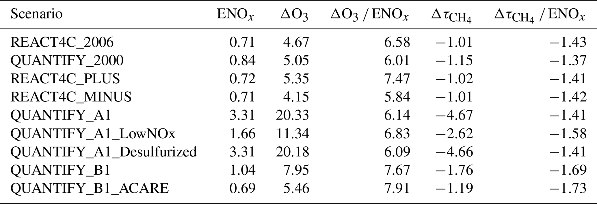
For the 2050 scenarios, ozone increases by up to 20.3 Tg (1.86 DU) for the QUANTIFY_A1 scenario and by 7–8 Tg (0.64–0.73 DU) for the B1 and B1_ACARE scenarios. Despite the very different atmospheric background in 2050, the derived ozone production efficiency for the A1 scenario (6.14) is rather close to the QUANTIFY_2000 reference value (6.0). A higher ozone production efficiency of 7.7 and 7.9 is derived in the case of the B1 and B1_ACARE scenarios, respectively. A similar feature was derived by Hodnebrog et al. (2011, 2012) for the QUANTIFY inventories in 2050, with ozone production efficiencies averaged among several models (and for different background conditions) of 5.7, 7.4, 7.9 for the A1, B1 and B1_ACARE scenarios, respectively. For the A1_LowNOx scenario (future NOx emissions reduced by 50 %), the ozone burden decreases by 56 % compared to the A1 scenario, showing a very slight non-linearity. We calculate a methane reference lifetime of 11.4 years in 2050. Due to aircraft emissions, the future methane lifetime decreases by 4.7 % for the QUANTIFY_A1 scenario and by 1.8 % and 1.2 % for the B1 and B1_ACARE scenarios, respectively. The calculated future ozone changes can also be compared with more recent estimates involving global models, including both tropospheric and stratospheric chemistry. With the ACCRI_2050_Base and 2050-S1 emissions (Table S2), Olsen et al. (2013) derived a global ozone burden increase ranging from 10.3 to 18.6 Tg (2.6–7.24 TgO3 TgN−1) and from 4.5 to 13.8 Tg (2.9–8.8 TgO3 TgN−1), respectively. More recently, using the MOZART-3 model and based on high (5.59 TgN) and low (2.17 TgN) future (2050) aircraft emission scenarios, Skowron et al. (2021) calculated the global ozone increases of 31 and 15.4 Tg with some variation depending on the surface emission scenario, providing 5.5 and 7.1 TgO3 TgN−1, respectively. Our results agree with the ozone sensitivity to NOx and all these future simulations point to a decreasing ozone production efficiency at higher NOx emissions. We re-emphasize that the impact of future climate change on aircraft perturbations is not considered in our simulations and should be investigated in forthcoming studies.
6.2 Radiative forcing (RF) from NOx emissions
The calculated RF of climate for the different scenarios are summarized in Table 5. The increase in tropospheric ozone due to the aircraft NOx emissions is responsible for a positive RF F of 15.9 mW m−2 in the case of the reference scenario REACT4C_2006. This forcing increases by 1.85 mW m−2 (12 %) when the flight altitude is increased in the case of REACT4C_PLUS and decreases by 1.59 mW m−2 (10 %) when the flight altitude is decreased in the case of REACT4C_MINUS. In the case of QUANTIFY_2000, the calculated ozone forcing is 17.2 mW m−2, a value somewhat higher than REACT4C_2006 due to higher NOx emissions. This value agrees with the ozone forcings calculated by Hoor et al. (2009) in a multi-model study; they derived a mean forcing of 16.3 mW m−2 for the QUANTIFY_2000 scenario. The calculated ozone forcing provides a forcing relative to the NOx emissions of 22.35 mW m−2 TgN−1. This value is in good agreement with Myhre et al. (2011), who calculated a range for five models of 16–25 mW m2 TgN−1 and Holmes et al. (2011), who calculated a forcing of 21.6±7.2 mW m−2 TgN−1 based on factor decomposition . As noted by Skowron et al. (2013), the ozone forcing is largely dependent on the NOx emission vertical profile with normalized forcings, ranging from 16.5 to 20.5 mW m−2 TgN−1 in their MOZART-3 simulations depending on the aircraft emission inventory considered. More recently, Lee et al. (2021) derived a best estimate value of 25.1±7.2 mW m−2 TgN−1. As obtained by Holmes et al. (2011), we derive an ozone forcing per DU of 37.1 mW m−2 DU−1, in agreement with this previous work (Table S4). With different emission inventories, Olsen et al. (2013) reported an even wider range for the normalized ozone forcing of 6–37 mW m−2 TgN−1. For the future scenarios, the tropospheric ozone forcing reaches 70.6 mW m−2 for the QUANTIFY_A1 scenario and 27.6 and 18.7 mW m−2 in the case of the B1 and B1_ACARE mitigation scenarios, respectively. These values agree with the ozone forcings calculated by Hodnebrog et al. (2011, 2012) in a multi-model study, who derived forcings of 61.3±14.0, 24.1±7.7 and 18.9±6.6 mW m−2 for the QUANTIFY_A1, QUANTIFY_B1 and B1_ACARE, respectively. For the reduced NOx emission scenario (A1_LowNOx), the ozone forcing is 55 % of the A1 scenario value, in line with the change in ozone burden.
Table 5Radiative forcings (RFs) of ozone, methane, black carbon (BC), sulfates, nitrates, organic carbon (OC) and stratospheric water vapour calculated for the different simulations (mW m−2). The RF of methane is the sum of 4 terms as depicted in Table 5.
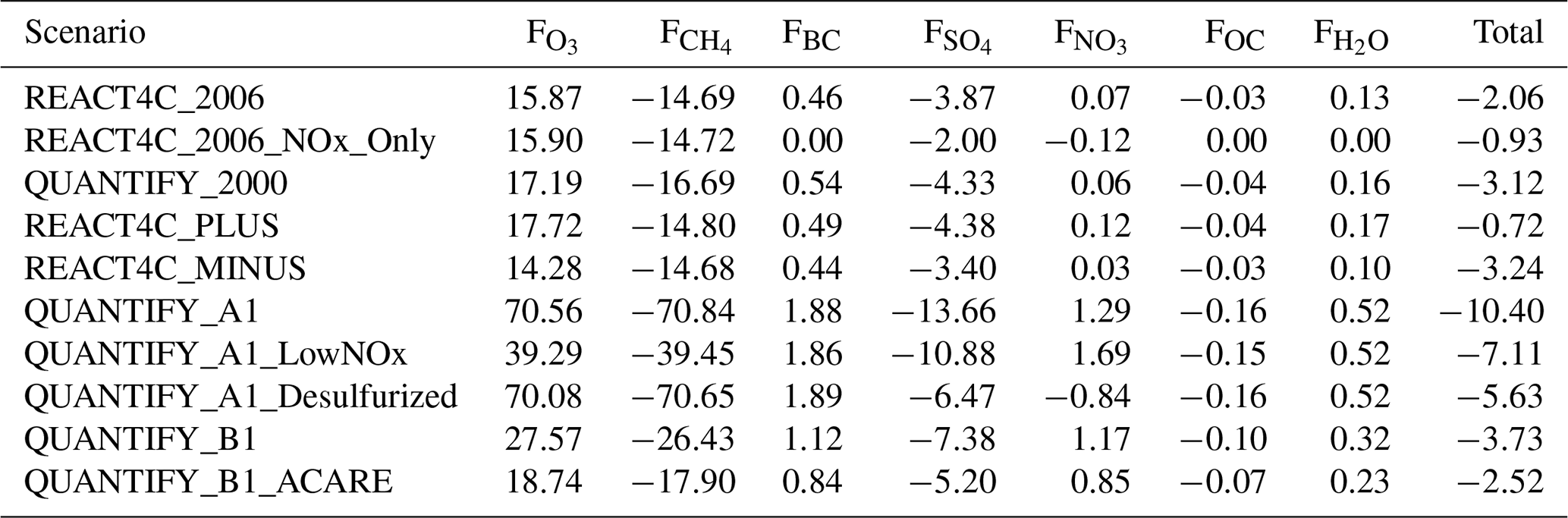
The total methane forcing F is broken down into four distinct forcings (Table 6). We calculate a direct RF at equilibrium associated with the methane decrease F of −11.0 mW m−2 for the present-day REACT4C_2006 simulation (−12.5 mW m−2 for the QUANTIFY_2000 simulation). For future conditions, the direct methane forcing ranges from −13.3 mW m−2 for the QUANTIFY_B1_ACARE to −52.8 mW m−2 for the QUANTIFY_A1 scenario. The indirect forcings associated with this change in methane mixing ratio through long-term tropospheric ozone (F) and stratospheric water vapour (F) adjustments, calculated for the REACT4C_2006 simulation are −2.82 and −0.65 mW m−2, respectively (−3.30 and −0.74 mW m−2, respectively, for the QUANTIFY_2000 simulation). For the future simulations, we calculate ozone long-term forcings F ranging from −3.6 mW m−2 (B1_ACARE) to −13.96 mW m−2 (A1), and a stratospheric water vapour forcings F ranging from −0.82 mW m−2 (B1_ACARE) to −3.22 mW m−2 (A1). The indirect RFs from CO2 production (F) are −0.20 and −0.23 mW m−2 for the present-day simulations REACT4C_2006 and QUANTIFY_2000, respectively, and range from −0.21 mW m−2(B1_ACARE) to −0.81 mW m−2 (A1) in 2050. The sum of these four components provides F the total methane RF associated with aircraft NOx emissions. This total forcing is −14.7 and −16.7 mW m−2 for the present-day REACT4C_2004 and QUANTIFY_2000 inventories, respectively. In 2050, the total methane forcing ranges from −17.9 mW m−2 for QUANTIFY_B1_ACARE to −70.8 mW m−2 for the A1 scenario (Table 6). The change in methane mixing ratio itself represents 75 % of this total methane forcing. The indirect changes through long-term tropospheric ozone, stratospheric water vapour and oxidation to CO2 contribute 19 %, 4 %, and 1 %, respectively.
Table 6Decomposition of the total methane forcing F into its various direct and indirect forcings. The forcings are associated with changes in methane lifetime (CH4−OH), tropospheric ozone production (CH4−O3), stratospheric water vapour production (CH4−SWV) and CO2 production (CH4−CO2) (mW m−2).
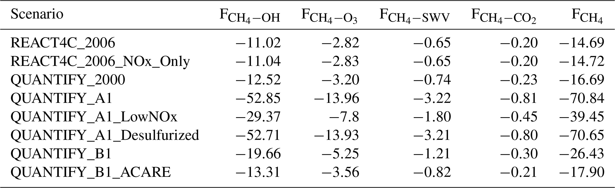
As seen in Table 5, the NOx forcing components resulting from the tropospheric ozone positive forcing and the methane negative forcing largely offset each other, resulting in a slightly positive forcing of 1.2 and 0.5 mW m−2 for the REACT4C_2006 and QUANTIFY_2000 present-day simulations, respectively. In 2050, a net negative forcing of −0.28 mW m−2 is calculated for the QUANTIFY_A1 scenario. For the alternative scenarios B1 and B1_ACARE, we still derive positive forcings of 1.14 and 0.84 mW m−2. This partial compensation and the resulting positive or negative NOx net forcing depends on the level of NOx present in the background atmosphere and the location of emissions (Stevenson and Derwent, 2009; Gilmore et al., 2013; Skowron et al., 2021). Thus, for the future, higher concentrations of NOx increase the OH response and the effect of methane so that even total NOx forcings become negative. Table S3 compares the methane forcings calculated with the revised CH4 RF parameterization proposed by Etminan et al. (2016) and by the former parameterization (Myhre et al., 1998). The net NOx negative forcings calculated for future conditions in this study are largely affected by this methane forcing parameterization. The methane forcing F is 23 % higher when the parameterization of Etminan et al. (2016) is used and the total methane forcing is about 15 % higher. In the case of the methane forcing former parameterization (Myhre et al., 1998), positive NOx net forcings ranging from 3.3–5.0 mW m−2 for present-day conditions to 3.3–9.7 mW m−2 in 2050 are calculated. A similar conclusion regarding the possibility to have negative NOx net forcings has been reached by Skowron et al. (2021). The RFs associated with NOx emissions are decomposed into its various factors following the methodology of Holmes et al. (2011) and compared to previous estimates in Table S4. A good agreement is found between the various components or sensitivities of the chemistry and the RFs with the previous estimate provided by Holmes et al. (2011). The major difference arises from the methane forcing calculation based on Etminan et al. (2016) in our study. Similarly, the forcings normalized by emissions are also generally in agreement with Lee et al. (2021).
The sensitivity of the NOx associated forcings with aircraft flight altitudes was investigated in earlier studies (Gauss et al., 2006; Frömming et al., 2012; Søvde et al., 2014). In particular, based on the REACT4C emission inventories, Søvde et al. (2014) derived, in a multi-model study, an increase of the total NOx forcing of 2±1 mW m−2 for aircraft cruising at higher altitudes and a decrease of the forcing by the same value for aircraft cruising at lower altitudes, with a change essentially due to the ozone forcing. In this study, the NOx net forcing is increased by 1.74 mW m−2 for aircraft cruising at higher altitudes and decreased by 1.58 mW m−2 at lower altitudes. These values agree with this previous estimate. It should be noted that, based on the parameterization of Etminan et al. (2016), the NOx net forcing turns from positive to negative when the aircraft cruise altitude is reduced (Table S3).
As illustrated by the REACT4C_2006_NOx_Only simulation results (only the NOx emissions are perturbed by aviation without including the other chemical and aerosol emissions) shown in Tables 5 and S4, additional forcings arise from aircraft NOx emissions. This sensitivity simulation shows that the change in OH associated with NOx emissions is responsible for an increased formation of sulfate particles and a negative forcing from these aerosols of −2.0 mW m−2. Similarly, NOx emissions and concentrations increase the formation of nitrate particles, also responsible for an additional negative forcing of −0.12 mW m−2. The nitrate forcing calculated by Pitari et al. (2016) is much higher (−1.7 mW m−2), but the role played by ammonia was not considered in this earlier study. It is important to consider the ammonium cycle because, as we discussed earlier, increased NOx from aircraft emissions increase nitrate particles in the lower troposphere. However, in the upper troposphere, increased sulfate concentrations will favour the titration of ammonia to form ammonium sulfates leading to lower ammonium nitrate concentrations despite the increased NOx and HNO3 concentrations. The total forcing of sulfate and nitrate aerosols associated with NOx emissions is −2.12 mW m−2. When these aerosol direct RFs are considered, the total net NOx forcing switches from a positive value of 1.19 mW m−2 for tropospheric ozone plus methane to −0.93 mW m−2. When these indirect terms are accounted for, we derive a negative net NOx RF per TgN emitted by aviation as summarized in Table S4. The inclusion of forcings associated with particles (SO4 and NO3) has been found to change the sign of the next NOx RFs compared to the earlier studies of Holmes et al. (2011) and Lee et al. (2021). It should be noted that the forcings associated with aerosols are of course subject to large uncertainties in the models (Lee et al., 2021; Forster et al., 2021) and more model simulations are needed in order to gain more confidence in these results.
It should also be noted that these two forcings from ozone and methane represent perturbations at a steady state. This assumption is correct for tropospheric ozone which has an average of a few weeks, but not for methane which has a lifetime of 10.6 years in our model. For methane, the response does not reach a steady state in any given year and the response in a particular year depends on the historical time-evolving emissions. This limitation was discussed and illustrated by Khodayari et al. (2014b), Grewe et al. (2019), Lee et al. (2021) and Matthes et al. (2021). For this reason, a transient correction factor was applied to the total methane forcing by Myhre et al. (2011), Hodnebrog et al. (2011, 2012), Matthes et al. (2021), and the best estimate value was provided by Lee et al. (2021). However, this factor was not considered in Brasseur et al. (2016) or, more recently, in Skowron et al. (2021). The major difficulty with this non-steady state factor is that its determination is strongly model dependent. Due to the long time integration needed to investigate the methane response, complex models have not been used to date, and the non-steady state factor was determined based on simplified or parameterized chemistry–climate models (Grewe and Stenke, 2008; Lee et al., 2021). Another difficulty in determining this factor, and in particular for future scenarios, arises from its dependency on the considered year or the assumed future emission pathway. For the QUANTIFY_2000 emissions, Myhre et al. (2011) derived, based on the methodology of Grewe and Stenke (2008), a non-steady state correction factor of 0.65. A similar factor was used by Matthes et al. (2021). This factor was recently reassessed by Lee et al. (2021) with a two-dimensional model and factors of 0.73 and 0.79 were determined for 2000 and 2018, respectively. For the future 2050 scenarios, Hodnebrog et al. (2011, 2012) derived factors of 0.74, 1.0, and 1.15 for the QUANTIFY A1B, B1, and B1_ACARE, respectively. Considering the uncertainty associated with this factor, the forcings calculated in this study assumed a steady-state methane perturbation, as was done by Skowron et al. (2021). However, for sake of completeness, Table S5 compares the standard steady-state forcings and the forcings with non-steady factors applied. The factors provided by Lee et al. (2021) for the 2000 and 2005 simulations and by Hodnebrog et al. (2011, 2012) for the 2050 scenarios were used. When these non-steady methane forcings are considered, the future NOx net forcings are generally higher and even switch back to positive in 2050. However, we are aware of the high uncertainty in these factors and the need for future work in order to provide a more robust estimate of this non-steady state correction and overall methodology.
6.3 Direct radiative forcing from SO2 and particulate carbon emissions
The concentrations of several types of particles are perturbed by aircraft emissions and hence provide direct RFs (Table 5). Direct emissions of soot particles induce a positive RF of 0.46 mW m−2 for the REACT4C_2006 inventory and 0.54 mW m−2 for the QUANTIFY_2000 inventory. With the REACT4C inventory, Pitari et al. (2015) calculated a higher direct soot forcing of 0.78 mW m−2. We note however that the soot RF is subject to large uncertainties. In 2050, this forcing reaches 1.88 mW m−2 for the QUANTIFY_A1 scenario. For these particles we derive a normalized forcing of 108–115 mW m−2 Tg−1 for present-day conditions, in the range provided by Balkanski et al. (2010) of 8–140 mW m−2 Tg−1 and calculated based on the QUANTIFY emissions. The calculated normalized forcing is also in good agreement with the recent study of Brasseur et al. (2016), providing a range of 101–168 mW m−2 Tg−1.
Sulfate particle concentrations are also perturbed by the aviation SO2 emissions and the direct SO4 emissions. The negative forcing associated with an increase of these particles largely dominates the effect of the other particles and ranges from −3.87 and −4.33 mW m−2 for the REACT4C_2006 and QUANTIFY_2000 present-day simulations to −13.7 mW m−2 in 2050 under the QUANTIFY_A1 scenario. With the REACT4C inventory, Pitari et al. (2015) calculated a direct sulfate forcing of −3.5 mW m−2, a value close to the one in this study. For these particles, we derive a normalized direct forcing of −52.8 (REACT4C_2006) and −49.3 (QUANTIFY_2000) mW m−2 TgS−1 for present-day conditions, in the range provided by Unger (2011) of −56 mW m−2 TgS−1 and Brasseur et al. (2016) of [] mW m−2 TgS−1. The atmospheric distribution of ammonium nitrate particles is indirectly affected by aviation emissions and dominated by the increase in sulfates favouring the formation of ammonium sulfates over ammonium nitrates. The decrease in nitrate particles is responsible for a positive forcing ranging from 0.07 mW m−2 for the present-day scenario to 1.3 mW m−2 in 2050 for the A1 scenario. The impact of aircraft emissions on nitrates largely depends on the NH3 and SO2 levels in the upper troposphere, as discussed by Unger et al. (2013), who calculated a much larger nitrate forcing from aircraft in their future simulations. The results of LMDZ-INCA showed a good comparison with other models as illustrated by the model intercomparison presented by Bian et al. (2017). A slight negative forcing reaching −0.16 mW m−2 in 2050 is associated with the emission of OC by aviation. In total, aerosols are responsible for a negative direct forcing largely dominated by sulfate particles and ranging from −3.4 mW m−2 in the case of REACT4C_2006 to −10.6 mW m−2 in 2050 for the A1 scenario.
The variation of aircraft flight altitudes modifies the residence time of particles in the atmosphere. A longer lifetime is associated with a higher injection altitude and therefore influences concentration changes and the RF associated with these particles. The forcing associated with soot particles increases from 0.46 mW m−2 for the REACT4C_2006 scenario to 0.49 mW m−2 at higher flight altitudes and decreases to 0.44 mW m−2 at lower altitudes. The dominant forcing from aviation-induced particles remains the negative forcing from sulfates. This forcing decreases from −3.87 to −4.38 mW m−2 at higher flight altitudes and increases to −3.40 mW m−2 at lower altitudes. The total aerosol forcing is dominated by sulfates and its variation with flight altitudes reflects the variation of the sulfate negative forcing. The total aerosol direct forcing decreases to −3.0 mW m−2 (−12 %) at lower flight altitudes (REACT4C_MINUS) and increases to −3.8 mW m−2 (+13 %) at higher flight altitudes (REACT4C_PLUS).
For the future QUANTIFY_A1 simulation, the use of desulfurized fuel reduces the sulfate direct forcing by 55 %. The remaining sulfate forcing is associated with changes in OH and increased sulfate formation. However, the reduced direct SO2 (and SO4) emissions have the consequence of decreasing the sulfate forcing to −6.5 mW m−2. The use of desulfurized fuel also has an impact on nitrate particles. In this case, the nitrates are essentially affected by increased NOx concentrations and a negative forcing of −0.8 mW m−2 is calculated. In total, the use of desulfurized fuel decreases the forcing of particles from −12.4 to −5.6 mW m−2. The ozone forcing is only slightly affected by the removal of SO2 aircraft emissions in agreement with Unger (2011).
6.4 Radiative forcing (RF) from water vapour emissions
The RF associated with water vapour increase in the stratosphere due to direct aircraft emissions and calculated with the LMDZ-INCA model is 0.13–0.16 mW m−2 for present-day conditions (REACT4C_2006 and QUANTIFY_2000) and increases to 0.52 mW m−2 in 2050 under the QUANTIFY_A1 scenario (Table 5). Based on earlier literature, Lee et al. (2009) reported a best estimate for this forcing of 2.8 mW m−2 with a range of 0.39–20.3 mW m−2. More recently, Lee et al. (2021) reported values ranging from 0.4 mW m−2 (Wilcox et al., 2012) to 1.5 mW m−2 (Frömming et al., 2012; Lim et al., 2015) and even to 3.0 mW m−2 (Penner et al., 1999), and derived a best estimate for this forcing of 2.0 (0.8, 3.2) mW m−2. The forcing recalculated with the LMDZ-INCA chemistry–transport model is at the lower range of this previous literature.
Myhre et al. (2009) performed an intercomparison of stratospheric water vapour RFs from several models imposing idealized stratospheric H2O perturbations. In particular, a simulation imposing an increase of water vapour in the stratosphere from 3 to 3.7 ppmv has been performed. In this case, based on six different models, the calculated net RFs at the tropopause ranged from 0.16 to 0.38 W m−2 with a mean at 0.25 W m−2. The long-wave forcings range from 0.19 to 0.40 W m−2 and the short-wave forcings range from −0.020 to −0.058 W m−2. In order to evaluate our radiative transfer model, we have performed this benchmark simulation with the LMDZ-INCA model version used in the present study. We calculate a net RF at the tropopause of 0.18 W m−2 (long-wave: 0.22 W m−2; short-wave: −0.038 W m−2). These forcings agree with the model ranges provided by Myhre et al. (2009) for both forcing components.
The water vapour forcing associated with aircraft emissions calculated in this study is based on a detailed calculation involving stratospheric chemistry and transport; it only includes the water vapour change above the tropopause. This forcing is at the lower range of previous estimates. It should be noted that these previous estimates are based on different model setups. For instance, Wilcox et al. (2012) used a Lagrangian model for transport imposing a water vapour lifetime, and Frömming et al. (2012) provided a water vapour forcing including both the H2O change in the stratosphere and upper troposphere. In Brasseur et al. (2016), the reported stratospheric water vapour forcings by two models (1.3 and 2.0 mW m−2) accounted for both direct H2O emissions and photochemical production by methane. A more detailed evaluation of this stratospheric water vapour forcing associated with direct aircraft emissions is still needed based on various models using the same protocol for calculation.
6.5 Total direct radiative forcing (RF) from atmospheric composition changes
The total RF from aircraft emissions and associated with changes in atmospheric chemistry and direct aerosols forcings are given in Table 5. The total forcing calculated with the LMDZ-INCA model are negative for both the present-day and future (2050) simulations. The total forcing ranges from −2.1 mW m−2 for the present-day inventory REACT4C_2006 (−3.1 mW m−2 in the case of the QUANTIFY_2000 inventory) to −2.5 mW m−2 in 2050 for the QUANTIFY_B1_ACARE scenario and −10.4 mW m−2 for the QUANTIFY_A1 scenario. A total negative forcing from reactive species and aerosol direct forcings was also calculated by Unger et al. (2013) for both present and future conditions based on the AEDT emission inventories. The total forcing associated with NOx-only emissions (REACT4C_2006_NOx_Only) also becomes negative (−0.93 mW m−2) when the indirect forcings from sulfate and nitrate particles are considered. The comparison with the baseline simulation (REACT4C_2006) indicates that the climate effect of NOx emissions amounts to about 45 % of the total perturbation. In the future simulations, this translates to a decrease of the total forcing by about 30 % when the NOx emissions are reduced by 50 %. Since sulfates dominate the particulate RF from aircraft, lowering the fuel sulfur content is another potential mitigation option to reduce the total forcing. For the future QUANTIFY_A1 simulation, the use of desulfurized fuel reduces the total forcing by more than 45 %.
The net effect of decreasing the flight cruise altitude by 2000 ft is to increase the total negative forcing from −2 to −3.2 mW m−2 (+57 %). Increasing the flight altitude by 2000 ft decreases the negative forcing to −0.7 mW m−2 (−65 %). The variation of the total forcing with flight altitude is dominated by the high sensitivity of the ozone positive forcing to the altitude of the perturbation, with the variation of the negative sulfate forcing being of secondary importance for these sensitivity simulations.
The RFs and ERFs from aircraft emissions calculated in this study are compared to the recent review by Lee et al. (2021) in Table 7. For this comparison, the forcings are scaled to the 2018 aircraft fuel and the ERF RF ratios provided by Lee et al. (2021) are applied to derive the ERF. For the methane forcing, we also apply the transient correction factor (see Sect. 6.2), recalculated and applied by Lee et al. (2021), for the best estimates (0.79). Overall, the agreement for the total forcing between this study and the best estimate from Lee et al. (2021), based on the previous literature, is reasonable. However, a detailed comparison shows that both the ozone positive and methane negative forcings are lower in LMDZ-INCA compared to the assessment by Lee et al. (2021), but remain in the 5 %–95 % uncertainty range provided in that study. The ozone forcing calculated in this study is in better agreement with the Holmes et al. (2011) best estimate as discussed earlier (see also Table S4). As indicated above, the stratospheric water vapour forcing is also significantly lower and requires further attention. Furthermore, it is important to note that the total ERF is now positive and equal to 8.9 mW m−2 (comparing well with the 8.6 mW m−2 best estimate from Lee et al., 2021), while the total RF calculated in Table 5 was negative (−2.06 mW m−2). This is due to the increase in Lee et al. (2021) of the ozone ERF by almost 40 % compared to the RF while keeping the aerosol forcings unchanged (ERF RF = 1). Considering the uncertainty in determining the ERF RF ratio for the different forcing agents, depending on the climate model used, this feature also clearly requires further investigation. A similar conclusion applies to the methane transient factor estimate.
Table 7Comparison of ozone, methane, black carbon (BC), sulfates, nitrates, organic carbon (OC), and stratospheric water vapour radiative forcings (RFs) and effective radiative forcings (ERFs) calculated for the REACT4C_2006 simulation and compared to Lee et al. (2021) (mW m−2). For this comparison, the REACT4C_2006 forcings are rescaled based on the total aviation fuel for 2018 and the ERF RF factors provided by Lee et al. (2021) are applied to derive the ERFs. For methane, the correction factor (0.79), recalculated by Lee et al. (2021) for the year 2018 to account for the non-steady state of CH4 responses to NOx emissions, is also applied. The RFs and ERFs from Lee et al. (2021) provide the median and 5 %–95 % confidence intervals, and the total forcings were recalculated based on a 106 Monte Carlo sampling from the discrete probability density function (PDF) provided by Lee et al. (2021).
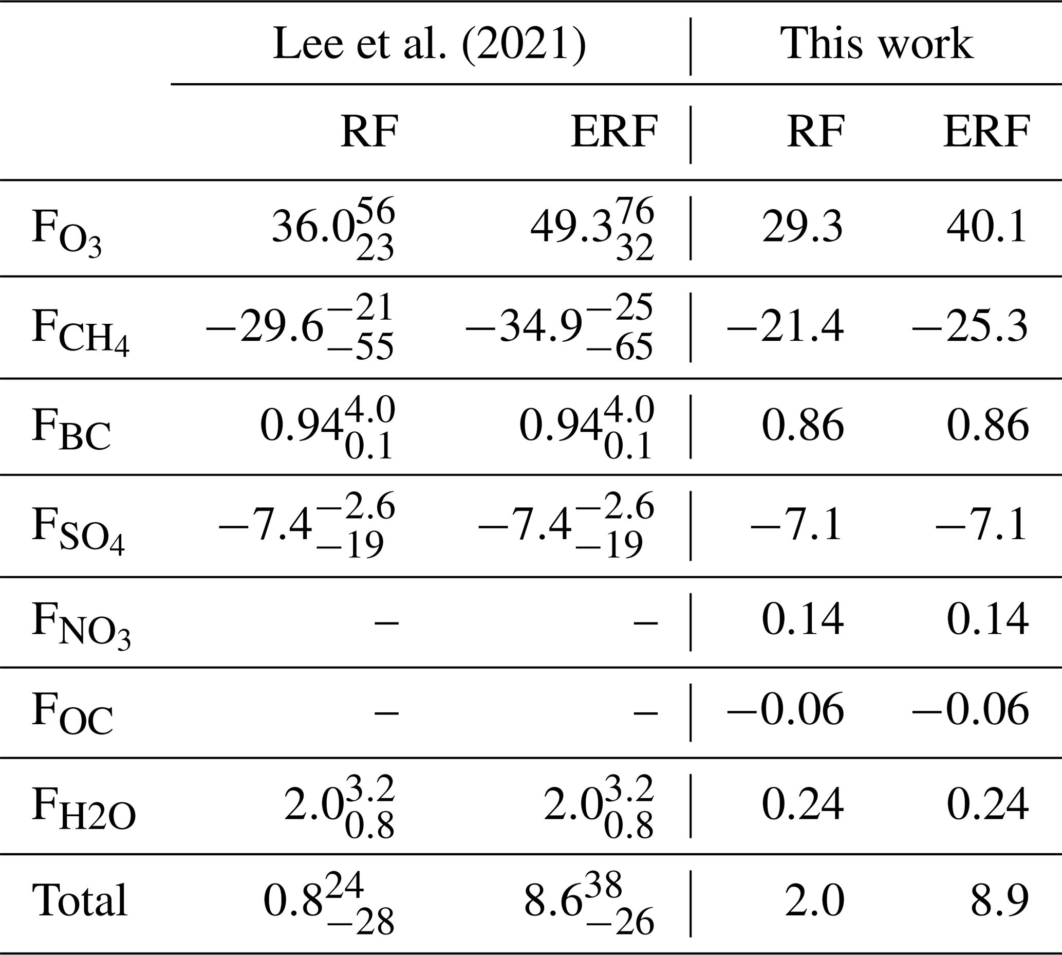
Aviation NOx emissions not only have an impact on global climate by changing ozone and methane levels in the atmosphere, but also contribute to the deterioration of local air quality. Improved combustor performance from future aircraft can not only contribute to reducing the impact of aircraft on climate but also provide a co-beneficial improvement of air quality. Historically however, reductions in aircraft NOx emissions have tended to increase fuel burn and hence CO2 emissions. Thus, a trade-off generally arises between reducing aircraft NOx and CO2 emissions. In order to properly assess the co-benefit with air quality improvement and the trade-off with climate change due to CO2 emissions, it appears essential to better quantify the climate impact of aircraft NOx emissions and its future evolution.
In this paper, a new version of the LMDZ-INCA global model is applied to re-evaluate the impact of aircraft NOx and aerosol emissions on climate. This version of the model is better designed to investigate the role played by aircraft emissions in the upper troposphere and lower stratosphere, including the gas-phase chemistry in both the troposphere and the stratosphere. The model results have been compared to ozone soundings and to IAGOS data for O3 and CO in the upper troposphere and lower stratosphere. In addition, tropospheric aerosols are also considered including the sulfate–nitrate–ammonium cycle and heterogeneous reactions between gas-phase chemistry and aerosols. With this model, we investigate the impact of present-day baseline and future (2050) aircraft emissions on atmospheric composition and the associated RFs of climate for ozone, methane and the aerosol direct forcings.
The key results from this study can be summarized as follows:
-
The results from the various simulations performed in this study confirm that the efficiency of NOx to produce ozone is largely dependent on the cruise altitude. Flying higher increases the impact of NOx on ozone and flying lower reduces the impact on ozone. In the future, an ozone production 4 times higher than that for the present-day simulation is calculated, i.e. an increase roughly linear with the increase in NOx emissions. The future evolution of the ozone production efficiency indicates that this efficiency increases with the background methane and NOx concentrations. The efficiency also increases with decreasing aircraft NOx emissions.
-
As a result of NOx aircraft emissions, the atmospheric methane sink is decreased by about 1 % for the present-day simulations and up to 4.7 % in 2050. We found that the methane lifetime variation is less sensitive to the location of the aircraft NOx emissions than the ozone change. Similarly, the methane sink appears slightly less sensitive to the amount of aircraft NOx emitted than the ozone production. This agrees with Holmes et al. (2011) and Skowron et al. (2021), who found ozone to be more responsive to aircraft emissions than methane. The net NOx forcing (O3+CH4) is largely affected by the revised CH4 RF formula provided by Etminan et al. (2016), which increases the total CH4 negative forcing by 15 %. As a consequence, the ozone positive forcing and the methane negative forcing largely offset each other, resulting in a slightly positive forcing for present-day simulations. In 2050, the net forcing even turns negative, essentially due to higher methane background concentrations. Skowron et al. (2021) also reached a similar conclusion that the revision of the methane RF significantly reduced the aircraft NOx forcing and that, in the future, this forcing could even turn negative, providing a different perspective of the impact that aircraft NOx emissions have on climate.
-
Additional RFs involving particle formation arise from aircraft NOx emissions and the sulfate–nitrate–ammonium cycle is also important to consider. The increased OH concentrations associated with NOx emissions are responsible for an enhanced conversion of SO2 to sulfate particles and an associated negative forcing. Aircraft NOx emissions also increase nitrate particles in the lower troposphere where ammonia concentrations are higher. In the upper troposphere, increased sulfate concentrations favour the titration of ammonia to form ammonium sulfates, leading to lower ammonium nitrate concentrations (despite the increased NOx and HNO3 concentrations). Overall, the indirect forcings of sulfate and nitrate aerosols associated with NOx emissions is negative and estimated to −3.0 mW m−2 TgN−1. When these aerosol RFs are considered, the net NOx forcing, due to O3 and CH4, and estimated to +2 mW m−2 TgN−1, turns from a positive value to a negative value, even for present-day conditions. The aerosol indirect forcings are subject to large uncertainties and are particularly sensitive to the model sulfate–ammonium–nitrate scheme (Unger et al., 2011; Righi et al., 2013; Pitari et al., 2016; Brasseur et al., 2016). Further investigation is clearly needed in order to gain more insight into these aircraft indirect forcings. Despite these uncertainties, the results suggest that, in addition to the increased methane negative forcing discussed above, indirect forcing from sulfate and nitrate particles could turn the aircraft NOx RF from positive to negative, not only for future scenarios, but also under present-day conditions.
-
The concentrations of several types of particles are perturbed by aircraft emissions and hence provide direct RFs of climate. The negative forcing associated with sulfates largely dominates the effect of the other particles. The sulfate direct RF is estimated to be associated with about 50 % of the direct SO2 and SO4 aircraft emissions and about 50 % of the increased conversion of SO2 to SO4 at higher OH concentrations, and hence related to the NOx emissions. In the future, the use of desulfurized fuel reduces the sulfate direct forcing and also has an impact on nitrate particles. Lowering the fuel sulfur content is therefore a potential mitigation option to reduce this aircraft negative forcing by more than 45 %. We found that the ozone forcing was only slightly affected by heterogeneous chemistry in the upper troposphere.
-
The RF associated with direct aircraft emissions of water vapour in the stratosphere is calculated in this study based on a detailed calculation involving stratospheric chemistry and transport; it only includes the water vapour change above the tropopause. This forcing is at the lower range of previous estimates. It should be noted that these previous estimates are based on very different model setups. This forcing is likely to be small; however, a more detailed evaluation of this stratospheric water vapour forcing associated with direct aircraft emissions is still needed based on several models using the same protocol for calculation.
-
Overall, the agreement for the non-CO2 total forcing between this study and the best estimate from Lee et al. (2021) is reasonable. However, a detailed comparison reveals several key differences and points to the key uncertainties associated with the NOx and aerosol direct forcings. Both the ozone positive and methane negative forcings are lower in LMDZ-INCA compared to the assessment of Lee et al. (2021), while remaining in the 5 %–95 % confidence range. This is mostly due to the increase in Lee et al. (2021) of the ozone ERF by almost 40 % compared to the RF while keeping the aerosol forcings unchanged (ERF RF = 1). Considering the uncertainty in the determination of the ERF RF ratio for the different forcing agents, depending on the climate model used, this feature clearly requires further investigation. A similar conclusion applies to the methane transient factor estimate which can flip the sign of the total NOx forcing.
-
Several previous studies have suggested that cruise emissions could be a significant or even dominant contribution to aviation-attributable surface level particulate matter and ozone (e.g. Barrett et al., 2010; Unger, 2011; Hauglustaine and Koffi, 2012; Lee et al., 2013; Eastham and Barrett, 2016). Our results confirm this important subsidence of ozone produced in the free troposphere by cruise altitude NOx emissions, down to the lower troposphere and surface. A similar downward transport of BC and sulfates is also simulated by the global model with a significant increase of particulate matter levels at the surface. We further find that aircraft NOx emissions are responsible, in the lower troposphere, for an important formation of ammonium nitrate particles, particularly in regions with high ammonia concentrations. Since ammonia concentrations are predicted to increase in the future (Hauglustaine et al., 2014), the aircraft NOx emissions could become a significant source of nitrate particles near the ground, in addition to already contributing significantly to ground-level sulfates and ozone concentrations.
These results show that several mitigation options involving aircraft flight operation and cruise altitude changes, traffic growth, engine technology, and fuel type, exist to reduce the climate impact of aircraft NOx emissions. However, our results, based on a current state-of-the-art global model, also show that the climate forcing of aircraft NOx emissions is likely to be small or even turn to negative (cooling), depending on atmospheric NOx or CH4 future background concentrations, and when the impact of aircraft NOx emissions on sulfate and nitrate particles is considered. Following previous work methodology, in order to better emphasize the impact of aircraft emissions on atmospheric composition, the impact of future climate change on aircraft perturbations is not considered in our simulations, performed based on a present-day, unchanged meteorology in 2050. The simulations performed by Olivié et al. (2012) and Huszar et al. (2013) accounted for future climate change; however, the impact of future climate on atmospheric composition changes due to aircraft emissions is not isolated. Changes in upper-tropospheric temperature, humidity, and dynamics have the potential to affect the response of the atmosphere to aircraft emissions. These perturbations are likely to be more pronounced at a longer time horizon than at the 2050 timeframe considered in our simulations, but this topic is clearly a subject to be investigated in forthcoming studies. There are still large uncertainties regarding the estimate of the aircraft NOx net impact on climate. In particular, the use of ERFs or accounting for the methane transient forcing varies among the different models. These methodological concepts also require further investigation in order to determine the best appropriate metric to express the climate impact of aircraft NOx. Large uncertainties remain regarding the NOx net impact on climate and particularly on the indirect forcings associated with aerosols, which are even more uncertain than the other forcings from gaseous species. Hence, additional studies with a range of models are needed in order to provide a more consolidated view. Nevertheless, the results seem to suggest that reducing aircraft NOx emissions is primarily beneficial for improving air quality and reducing ground-level O3 and particulate matter (PM) concentrations. New technologies in combustor design, which could help to simultaneously reduce NOx and CO2 emissions, do not appear to be essential for aircraft non-CO2 climate mitigation, but can be co-beneficial for climate change mitigation from CO2 emission reduction and air quality improvement from reduced aviation NOx emissions.
The LMDZ-INCA global model is part of the Institut Pierre Simon Laplace (IPSL) Climate Modelling Center Coupled Model. The documentation on the code and the code itself can be found at https://cmc.ipsl.fr/ipslclimate-models/ipsl-cm6/ (IPSL, 2022). The Python codes used for analysing the data and plotting the analysed data are available from the corresponding author upon reasonable request. The distribution of the IAGOS data onto LMDZ-INCA grids is based on an updated version of the Interpol-IAGOS software, available at https://doi.org/10.25326/81 (Cohen et al., 2020).
To access datasets of LMDZ-INCA results, please contact Didier Hauglustaine. The IAGOS data set can be found at https://doi.org/10.25326/20 (IAGOS, 2022).
The supplement related to this article is available online at: https://doi.org/10.5194/acp-22-11987-2022-supplement.
DAH and ET set up the LMDZ-INCA model simulations and analysed and post-processed the LMDZ-INCA model results. DAH calculated the radiative forcings. YC contributed to the LMDZ-INCA model valuation. AC is involved in the development of the INCA model and its coupling with the LMDZ model. RV and FL contributed to the development of the INCA model version used in this study. SM was involved in the discussion of the results and supported the writing of the document. The manuscript was written by DAH, then reviewed by the authors and approved by all the authors.
The contact author has declared that none of the authors has any competing interests.
Publisher's note: Copernicus Publications remains neutral with regard to jurisdictional claims in published maps and institutional affiliations.
We thank Yunjiang Zhang for preparing the model aerosol optical depth evaluation against MODIS and AERONET data. The simulations were performed using HPC resources from GENCI (Grand Equipement National de Calcul Intensif).
This study was partly funded by the Direction Générale de l’Aviation Civile (DGAC) under the IMPACT and CLIMAVIATION projects and by the European Union Horizon 2020 research and innovation programme under the ACACIA project (grant agreement no. 875036).
This paper was edited by Holger Tost and reviewed by two anonymous referees.
Balkanski, Y., Myhre, G., Gauss, M., Rädel, G., Highwood, E. J., and Shine, K. P.: Direct radiative effect of aerosols emitted by transport: from road, shipping and aviation, Atmos. Chem. Phys., 10, 4477–4489, https://doi.org/10.5194/acp-10-4477-2010, 2010.
Barrett, S. R. H., Britter, R. E., and Waitz, I. A.: Global mortality attributable to aircraft cruise emissions, Environ. Sci. Technol., 44, 7736–7742, https://doi.org/10.1021/es101325r, 2010.
Bauer, S., Balkanski, Y., Schulz, M., Hauglustaine, D. A., and Dentener, F.: Heterogeneous chemistry on mineral aerosol surfaces: a global modelling study on the influence on tropospheric ozone chemistry and comparison to observations, J. Geophys. Res., 109, D02304, https://doi.org/10.1029/2003JD003868, 2004.
Berntsen, T. K., Fuglestvedt, J. S., Joshi, M., Shine, K. P., Stuber, N., Ponater, M., Sausen, R., Hauglustaine, D. A., and Li, L.: Climate response to regional emissions of ozone precursors; sensitivities and warming potentials, Tellus B, 57, 283–304, 2005.
Bian, H., Chin, M., Hauglustaine, D. A., Schulz, M., Myhre, G., Bauer, S. E., Lund, M. T., Karydis, V. A., Kucsera, T. L., Pan, X., Pozzer, A., Skeie, R. B., Steenrod, S. D., Sudo, K., Tsigaridis, K., Tsimpidi, A. P., and Tsyro, S. G.: Investigation of global particulate nitrate from the AeroCom phase III experiment, Atmos. Chem. Phys., 17, 12911–12940, https://doi.org/10.5194/acp-17-12911-2017, 2017.
Boucher, O., Friedlingstein, P., Collins, B., and Shine, K. P.: The indirect global warming potential and global temperature change potential due to methane oxidation, Environ. Res. Lett., 4, 4, https://doi.org/10.1088/1748-9326/4/4/044007, 2009.
Boucher, O., Servonnat, J., Albright, A. L., Aumont, O., Balkanski, Y., Bastrikov, V., Bekki, S., Bonnet, R., Bony, S., Bopp, L., Braconnot, P., Brockmann, P., Cadule, P., Caubel, A., Cheruy, F., Codron, F., Cozic, A., Cugnet, D., D'Andrea, P., Davini, de Lavergne, C., Denvil, S., Deshayes, J., Devilliers, M., Ducharne, A., Dufresne, J.-L., Dupont, E., Éthé, C., Fairhead, L., Falletti, F., Flavoni, S., Foujols, M.-A., Gardoll, S., Gastineau, G., Ghattas, J., Grandpeix, J.-Y., Guenet, B., Guez, L., Guilyardi, E., Guimberteau, M., Hauglustaine, D., Hourdin, F., Idelkadi, A., Joussaume, S., Kageyama, M., Khodri, M., Krinner, G., Lebas, N., Levavasseur, G., Lévy, C., Li, L., Lott, F., Lurton, T., Luyssaert, S., Madec, G., Madeleine, J. B., Maignan, F., Marchand, M., Marti, O., Mellul, L., Meurdesoif, Y., Mignot, J., Musat, I., Ottlé, C., Peylin, P., Planton, Y., Polcher, J., Rio, C., Rochetin, N., Rousset, C., Sepulchre, P., Sima, A., Swingedouw, D., Thiéblemont, R., Traore, A., K., Vancoppenolle, M., Vial, J., Vialard, J., Viovy, N., and Vuichard, N.: Presentation and evaluation of the IPSL-CM6A-LR climate model, J. Adv. Model. Earth Sy., 12, e2019MS002010. https://doi.org/10.1029/2019MS002010, 2020.
Boucher, O., Borella, A., Gasser, T., and Hauglustaine, D.: On the contribution of global aviation to the CO2 radiative forcing of climate, Atmos. Environ., 267, 118761, https://doi.org/10.1016/j.atmosenv.2021.118762, 2021.
Bousquet, P., Yver, C., Pison, I., Li, Y. S., Fortems, A., Hauglustaine, D., Szopa, S., Rayner, P. J., Novelli, P., Langenfelds, R., Steele, P., Ramonet, M., Schmidt, M., Foster, P., Morfopulos, C., and Ciais, P.: A 3D synthesis inversion of the molecular hydrogen cycle: sources and sinks budget implications for the soil uptake, J. Geophys. Res., 116, D01302, https://doi.org/10.1029/2010JD014599, 2011.
Bouwman, A. F., Lee, D. S., Asman, W. A. H., Dentener, F. J., Van Der Hoek, K. W., and Olivier, J. G. J.: A global high-resolution emission inventory for ammonia, Global Biogeochem. Cycles, 11, 561–587, 1997.
Brasseur, G. P., Cox, R. A., Hauglustaine, D. A., Isaksen, I., Lelieveld, J., Lister, D. H., Sausen, R., Schumann, U., Wahner, A., and Wiesen, P.: European scientific assessment of the atmospheric effects of aircraft emissions, Atmos. Environ., 32, 2329–2418, 1998.
Brasseur, G. P., Gupta, M., Anderson, B. E., Balasubramanian, S., Barrett, S., Duda, D., Fleming, G., Forster, P. M., Fuglestvedt, J., Gettelman, A., Halthore, R. N., Jacob, S. D., Jacobson, M. Z., Khodayari, A., Liou, K.-N., Lund, M. T., Miake-Lye, R. C., Minnis, P., Olsen, S., Penner, J. E., Prinn, R., Schumann, U., Selkirk, H. B., Sokolov, A., Unger, N., Wolfe, P., Wong, H.-W., Wuebbles, D. W., Yi, B., Yang, P., and Zhou, C.: Impact of aviation on climate, B. Am. Meteorol. Soc., 97, 561–583, https://doi.org/10.1175/BAMS-D-13-00089.1, 2016.
Brunner, D., Staehelin, J., Rogers, H. L., Köhler, M. O., Pyle, J. A., Hauglustaine, D., Jourdain, L., Berntsen, T. K., Gauss, M., Isaksen, I. S. A., Meijer, E., van Velthoven, P., Pitari, G., Mancini, E., Grewe, G., and Sausen, R.: An evaluation of the performance of chemistry transport models by comparison with research aircraft observations. Part 1: Concepts and overall model performance, Atmos. Chem. Phys., 3, 1609–1631, https://doi.org/10.5194/acp-3-1609-2003, 2003.
Brunner, D., Staehelin, J., Rogers, H. L., Köhler, M. O., Pyle, J. A., Hauglustaine, D. A., Jourdain, L., Berntsen, T. K., Gauss, M., Isaksen, I. S. A., Meijer, E., van Velthoven, P., Pitari, G., Mancini, E., Grewe, V., and Sausen, R.: An evaluation of the performance of chemistry transport models – Part 2: Detailed comparison with two selected campaigns, Atmos. Chem. Phys., 5, 107–129, https://doi.org/10.5194/acp-5-107-2005, 2005.
Cameron, M. A., Jacobson, M. Z., Barrett, S. R. H., Bian, H., Chen, C. C., Eastham, S. D., Gettelman, A., Khodayari, A., Liang, Q., Selkirk, H. B., Unger, N., Wuebbles, D. J., and Yue, X.: An intercomparative study of the effects of aircraft emissions on surface air quality, J. Geophys. Res. 122, 8325–8344, https://doi.org/10.1002/2016JD025594, 2017.
Carslaw, K., Luo, B., and Peter, T.: An analytic expression for the composite of aqueous HNO3 -H2SO4 stratospheric aerosols including gas phase removal of HNO3, Geophys. Res. Lett., 22, 1877–1880, 1995.
Clappier, A., Belis, C. A., Pernigotti, D., and Thunis, P.: Source apportionment and sensitivity analysis: two methodologies with two different purposes, Geosci. Model Dev., 10, 4245–4256, https://doi.org/10.5194/gmd-10-4245-2017, 2017.
Cohen, Y., Petetin, H., Thouret, V., Marécal, V., Josse, B., Clark, H., Sauvage, B., Fontaine, A., Athier, G., Blot, R., Boulanger, D., Cousin, J.-M., and Nédélec, P.: Climatology and long-term evolution of ozone and carbon monoxide in the upper troposphere–lower stratosphere (UTLS) at northern midlatitudes, as seen by IAGOS from 1995 to 2013, Atmos. Chem. Phys., 18, 5415–5453, https://doi.org/10.5194/acp-18-5415-2018, 2018.
Cohen, Y., Marecal, V., Thouret, V., Josse, B., and Boulanger, D.: Interpol-IAGOS software, Aeris [software], https://doi.org/10.25326/81 (last access: 12 September 2022), 2020.
Cohen, Y., Marécal, V., Josse, B., and Thouret, V.: Interpol-IAGOS: a new method for assessing long-term chemistry–climate simulations in the UTLS based on IAGOS data, and its application to the MOCAGE CCMI REF-C1SD simulation, Geosci. Model Dev., 14, 2659–2689, https://doi.org/10.5194/gmd-14-2659-2021, 2021.
Collins, W. J., Lamarque, J.-F., Schulz, M., Boucher, O., Eyring, V., Hegglin, M. I., Maycock, A., Myhre, G., Prather, M., Shindell, D., and Smith, S. J.: AerChemMIP: quantifying the effects of chemistry and aerosols in CMIP6, Geosci. Model Dev., 10, 585–607, https://doi.org/10.5194/gmd-10-585-2017, 2017.
Dahlmann, K, Grewe, V., Ponater, M., and Matthes, S.: Quantifying the contributions of individual NOx sources to the trend in ozone radiative forcing, Atmos. Environ, 45, 2860–2868, https://doi.org/10.1016/j.atmosenv.2011.02.071, 2011.
Derwent, R. G., Collins, W. J., Johnson, C. E., and Stevenson, D. S.: Transient behaviour of tropospheric ozone precursors in a global 3-D CTM and their indirect greenhouse effects, Climatic Change, 49, 463–487, https://doi.org/10.1023/A:1010648913655, 2001.
Eastham, S. D. and Barrett, S. R. H.: Aviation-Attributable Ozone as a Driver for Changes in Mortality Related to Air Quality and Skin Cancer, Atmos. Environ., 144, 17–23, https://doi.org/10.1016/j.atmosenv.2016.08.040, 2016.
Emanuel, K. A.: A scheme for representing cumulus convection in large-scale models, J. Atmos. Sci., 48, 2313–2335, 1991.
Etminan, M., Myhre, G., Highwood, E. J., and Shine, K. P.: Radiative forcing of carbon dioxide, methane, and nitrous oxide: A significant revision of the methane radiative forcing, Geophys. Res. Lett., 43, 12614–12623, https://doi.org/10.1002/2016GL071930, 2016.
Eyers, C. J., Addleton, D., Atkinson, K., Broomhead, M. J., Christou, R., Elliff, T., Falk, R., Gee, I., Lee, D. S., Marizy, C., Michot, S., Middel, J., Newton, P., Norman, P., Plohr, M., Raper, D., and Stanciou, N.: AERO2K Global Aviation Emissions Inventories for 2002 and 2025, QINETIQ/04/01113, Farnborough, Hants, UK, https://www.yumpu.com/en/document/view/7313363/aero2k-global-aviation-emissions-inventories-for-2002-and-2025 (last access: 7 September 2022), 2005.
Federal Aviation Administration (FAA): Recommended best practice for quantifying speciated organic gas emissions from aircraft equipped with turbofan, turbojet and turboprop engines, https://nepis.epa.gov/Exe/ZyNET.exe/P1003YX3 (last access: 7 September 2022), 2009.
Fiore, A. M., Dentener, F. J., Wild, O., Cuvelier, C., Schultz, M. G., Hess, P., Textor, C., Schulz, M., Doherty, R. M., Horowitz, L. W., MacKenzie, I. A., Sanderson, M. G., Shindell, D. T., Stevenson, D. S., Szopa, S., Van Dingenen, R., Zeng, G., Atherton, C., Bergmann, D., Bey, I., Carmichael, G., Collins, W. J., Duncan, B. N., Faluvegi, G., Folberth, G., Gauss, M., Gong, S., Hauglustaine, D., Holloway, T., Isaksen, I. S. A., Jacob, D. J., Jonson, J. E., Kaminski, J. W., Keating, T. J., Lupu, A., Marmer, E., Montanaro, V., Park, R. J., Pitari, G., Pringle, K. J., Pyle, J. A., Schroeder, S., Vivanco, M. G., Wind, P., Wojcik, G., Wu, S., and Zuber, A.: Multimodel estimates of intercontinental source-receptor relationships for ozone pollution, J. Geophys. Res., 114, D04301. https://doi.org/10.1029/2008JD010816, 2009.
Folberth, G. A., Hauglustaine, D. A., Ciais, P., and Lathière, J.: On the role of atmospheric chemistry in the global CO2 budget, Geophys. Res. Lett, 32, L08801, https://doi.org/10.1029/2004GL021812, 2005.
Folberth, G. A., Hauglustaine, D. A., Lathière, J., and Brocheton, F.: Interactive chemistry in the Laboratoire de Météorologie Dynamique general circulation model: model description and impact analysis of biogenic hydrocarbons on tropospheric chemistry, Atmos. Chem. Phys., 6, 2273–2319, https://doi.org/10.5194/acp-6-2273-2006, 2006.
Forster, P., Storelvmo, T., Armour, K., Collins, W., Dufresne, J.-L., Frame, D., Lunt, D. J., Mauritsen, T., Palmer, M. D., Watanabe, M., Wild, M., and Zhang, H.: 2021: The Earth's Energy Budget, Climate Feedbacks, and Climate Sensitivity, in: Climate Change 2021: The Physical Science Basis. Contribution of Working Group I to the Sixth Assessment Report of the Intergovernmental Panel on Climate Change, edited by: Masson-Delmotte, V., Zhai, P., Pirani, A., Connors, S. L., Péan, C., Berger, S., Caud, N., Chen, Y., Goldfarb, L., Gomis, M. I., Huang, M., Leitzell, K., Lonnoy, E., Matthews, J. B. R., Maycock, T. K., Waterfield, T., Yelekçi, O., Yu, R., and Zhou, B., Cambridge University Press, Cambridge, United Kingdom and New York, NY, USA, 923–1054, https://doi.org/10.1017/9781009157896.009, 2021.
Fouquart, Y. and Bonel, B.: Computations of solar heating of the earth's atmosphere: a new parameterization, Beitr. Phys. Atmos., 53, 35–62, 1980.
Freeman, S., Lee, D. S., Lim, L. L., Skowron, A., and De Leon, R. R.: Trading off aircraft fuel burn and NOx emissions for optimal climate policy, Environ. Sci. Technol. 52, 2498–2505, 2018.
Frömming, C., Ponater, M., Dahlmann, K., Grewe, V., Lee, D. S., and Sausen, R.: Aviation-induced radiative forcing and surface temperature change in dependency of the emission altitude, J. Geophys. Res., 117, D19104, https://doi.org/10.1029/2012JD018204, 2012.
Fuglestvedt, J. S., Berntsen, T. K., Isaksen, I. S. A., Mao, H. T., Liang, X. Z., and Wang, W. C.: Climatic forcing of nitrogen oxides through changes in tropospheric ozone and methane; global 3D model studies, Atmos. Environ., 33, 961–977, 1999.
Gauss, M., Isaksen, I. S. A., Lee, D. S., and Søvde, O. A.: Impact of aircraft NOx emissions on the atmosphere – tradeoffs to reduce the impact, Atmos. Chem. Phys., 6, 1529–1548, https://doi.org/10.5194/acp-6-1529-2006, 2006.
Gilmore, C. K., Barrett, S. R. H., Koo, J., and Wang, Q.: Temporal and spatial variability in the aviation NOx-related O3 impact, Environ. Res. Lett., 8, 034027, https://doi.org/10.1088/1748-9326/8/3/034027, 2013.
Gliß, J., Mortier, A., Schulz, M., Andrews, E., Balkanski, Y., Bauer, S. E., Benedictow, A. M. K., Bian, H., Checa-Garcia, R., Chin, M., Ginoux, P., Griesfeller, J. J., Heckel, A., Kipling, Z., Kirkevåg, A., Kokkola, H., Laj, P., Le Sager, P., Lund, M. T., Lund Myhre, C., Matsui, H., Myhre, G., Neubauer, D., van Noije, T., North, P., Olivié, D. J. L., Rémy, S., Sogacheva, L., Takemura, T., Tsigaridis, K., and Tsyro, S. G.: AeroCom phase III multi-model evaluation of the aerosol life cycle and optical properties using ground- and space-based remote sensing as well as surface in situ observations, Atmos. Chem. Phys., 21, 87–128, https://doi.org/10.5194/acp-21-87-2021, 2021.
Grewe, V., Dameris, M., Fichter, C., and Lee, D.: Impact of aircraft NOx emissions. Part 2: Effects of lowering the flight altitude, Meteorol. Z., 3, 197–205, 2002.
Grewe, V. and Stenke, A.: AirClim: an efficient tool for climate evaluation of aircraft technology, Atmos. Chem. Phys., 8, 4621–4639, https://doi.org/10.5194/acp-8-4621-2008, 2008.
Grewe, V., Frömming, C., Matthes, S., Brinkop, S., Ponater, M., Dietmüller, S., Jöckel, P., Garny, H., Tsati, E., Dahlmann, K., Søvde, O. A., Fuglestvedt, J., Berntsen, T. K., Shine, K. P., Irvine, E. A., Champougny, T., and Hullah, P.: Aircraft routing with minimal climate impact: the REACT4C climate cost function modelling approach (V1.0), Geosci. Model Dev., 7, 175–201, https://doi.org/10.5194/gmd-7-175-2014, 2014.
Grewe, V., Matthes, S., and Dahlmann, K.: The contribution of aviation NOx to climate change: are we ignoring methodological flaws?, Environ. Res. Lett., 14, 121003, https://doi.org/10.1088/1748-9326/ab5dd7, 2019.
Hanson, D., Ravishankara, A. R., and Solomon, S.: Heterogeneous reactions in sulfuric acid aerosols: A framework for model calculations, J. Geophys. Res., 99, 3615–3629, 1988.
Hauglustaine D. A., Granier, C., Brasseur G. P., and Mégie, G.: Impact of present aircraft emissions of nitrogen oxides on tropospheric ozone and climate forcing, Geophys. Res. Lett., 21, 2031–2034, 1994.
Hauglustaine, D. A., Hourdin, F., Jourdain, L., Filiberti, M. A., Walters, S., Lamarque, J. F., and Holland, E. A.: Interactive chemistry in the Laboratoire de Meteorologie Dynamique general circulation model: Description and background tropospheric chemistry evaluation, J. Geophys. Res., 109, D04314, https://doi.org/10.1029/2003JD003957, 2004.
Hauglustaine, D. A. and Koffi, B.: Boundary layer ozone pollution caused by future aircraft emissions, Geophys. Res. Lett., 39, L13808, https://doi.org/10.1029/2012GL052008, 2012.
Hauglustaine, D. A., Balkanski, Y., and Schulz, M.: A global model simulation of present and future nitrate aerosols and their direct radiative forcing of climate, Atmos. Chem. Phys., 14, 11031–11063, https://doi.org/10.5194/acp-14-11031-2014, 2014.
Hodnebrog, Ø., Berntsen, T. K., Dessens, O., Gauss, M., Grewe, V., Isaksen, I. S. A., Koffi, B., Myhre, G., Olivié, D., Prather, M. J., Pyle, J. A., Stordal, F., Szopa, S., Tang, Q., van Velthoven, P., Williams, J. E., and Ødemark, K.: Future impact of non-land based traffic emissions on atmospheric ozone and OH – an optimistic scenario and a possible mitigation strategy, Atmos. Chem. Phys., 11, 11293–11317, https://doi.org/10.5194/acp-11-11293-2011, 2011.
Hodnebrog, Ø., Berntsen, T. K., Dessens, O., Gauss, M., Grewe, V., Isaksen, I. S. A., Koffi, B., Myhre, G., Olivié, D., Prather, M. J., Stordal, F., Szopa, S., Tang, Q., van Velthoven, P., and Williams, J. E.: Future impact of traffic emissions on atmospheric ozone and OH based on two scenarios, Atmos. Chem. Phys., 12, 12211–12225, https://doi.org/10.5194/acp-12-12211-2012, 2012.
Hoesly, R. M., Smith, S. J., Feng, L., Klimont, Z., Janssens-Maenhout, G., Pitkanen, T., Seibert, J. J., Vu, L., Andres, R. J., Bolt, R. M., Bond, T. C., Dawidowski, L., Kholod, N., Kurokawa, J.-I., Li, M., Liu, L., Lu, Z., Moura, M. C. P., O'Rourke, P. R., and Zhang, Q.: Historical (1750–2014) anthropogenic emissions of reactive gases and aerosols from the Community Emissions Data System (CEDS), Geosci. Model Dev., 11, 369–408, https://doi.org/10.5194/gmd-11-369-2018, 2018.
Holmes, C. D.: Methane feedback on atmospheric chemistry: Methods, models, and mechanisms, J. Adv. Model. Earth Sy., 10, 1087–1099, https://doi.org/10.1002/2017MS001196, 2018.
Holmes, C. D., Tang, Q., and Prather, M.: Uncertainties in climate assessment for the case of aviation NO, P. Natl. Acad. Sci. USA, 108, 10997–11002, 2011.
Hoor, P., Borken-Kleefeld, J., Caro, D., Dessens, O., Endresen, O., Gauss, M., Grewe, V., Hauglustaine, D., Isaksen, I. S. A., Jöckel, P., Lelieveld, J., Myhre, G., Meijer, E., Olivie, D., Prather, M., Schnadt Poberaj, C., Shine, K. P., Staehelin, J., Tang, Q., van Aardenne, J., van Velthoven, P., and Sausen, R.: The impact of traffic emissions on atmospheric ozone and OH: results from QUANTIFY, Atmos. Chem. Phys., 9, 3113–3136, https://doi.org/10.5194/acp-9-3113-2009, 2009.
Hourdin, F. and Armengaud, A.: The use of finite-volume methods for atmospheric advection of trace species 1. Test of various formulations in a general circulation model, Mon. Weather Rev., 127, 822–837, 1999.
Hourdin, F. and Issartel, J. P., Sub-surface nuclear tests monitoring through the CTBT xenon network, Geophys. Res. Lett., 27, 2245–2248, 2000.
Hourdin, F., Grandpeix, J.-Y., Madeleine, J.-B., Chéruy, F., Rochetin, N., Musat, I., Idelkadi, A., Fairhead, L., Foujols, M.-A., Mellul, L., Traore, A.-K., Dufresne, J.-L., Boucher, O., Lefebvre, M.-P., Millour, E., Vignon, E., Jouaud, J., Diallo, F. B., Lott, F., Caubel, A., Meurdesoif, Y., and Ghattas, J.: LMDZ6A: the atmospheric component of the IPSL climate model with improved and better tuned physics, J. Adv. Model. Earth Sy., 12, e2019MS001892, https://doi.org/10.1029/2019MS001892, 2020.
Huszar, P., Teyssèdre, H., Michou, M., Voldoire, A., Olivié, D. J. L., Saint-Martin, D., Cariolle, D., Senesi, S., Salas Y Melia, D., Alias, A., Karcher, F., Ricaud, P., and Halenka, T.: Modeling the present and future impact of aviation on climate: an AOGCM approach with online coupled chemistry, Atmos. Chem. Phys., 13, 10027–10048, https://doi.org/10.5194/acp-13-10027-2013, 2013.
IAGOS: IAGOS, In-service Aircraft for a Global Observing System, Aeris, https://doi.org/10.25326/20, 2022.
Institut Pierre Simon Laplace (IPSL): Climate Modelling Center Coupled Model, https://cmc.ipsl.fr/ipslclimate-models/ipsl-cm6/, last access: 12 September 2022.
Ivanovich, C. C., Ocko, I. B., Piris-Cabezas, P., and Petsonk, A.: Climate benefits of proposed carbon dioxide mitigation strategies for international shipping and aviation, Atmos. Chem. Phys., 19, 14949–14965, https://doi.org/10.5194/acp-19-14949-2019, 2019.
Jourdain, L. and Hauglustaine, D. A.: The global distribution of lightning NOx simulated on-line in a general circulation model, Phys. Chem. Earth, 26, 585–591, 2001.
Kapadia, Z. Z., Spracklen, D. V., Arnold, S. R., Borman, D. J., Mann, G. W., Pringle, K. J., Monks, S. A., Reddington, C. L., Benduhn, F., Rap, A., Scott, C. E., Butt, E. W., and Yoshioka, M.: Impacts of aviation fuel sulfur content on climate and human health, Atmos. Chem. Phys., 16, 10521–10541, https://doi.org/10.5194/acp-16-10521-2016, 2016.
Kärcher, B.: Formation and radiative forcing of contrail cirrus, Nat. Commun., 9, 1824, https://doi.org/10.1038/s41467-018-04068-0, 2018.
Khodayari, A., Tilmes, S., Olsen, S. C., Phoenix, D. B., Wuebbles, D. J., Lamarque, J.-F., and Chen, C.-C.: Aviation 2006 NOx-induced effects on atmospheric ozone and HOx in Community Earth System Model (CESM), Atmos. Chem. Phys., 14, 9925–9939, https://doi.org/10.5194/acp-14-9925-2014, 2014a.
Khodayari, A., Olsen, S. C., and Wuebbles, D. J.: Evaluation of aviation NOx-induced radiative forcings for 2005 and 2050, Atmos. Environ., 91, 95–103, https://doi.org/10.1016/j.atmosenv.2014.03.044, 2014b.
Khodayari, A., Olsen, S. C., Wuebbles, D. J., and Phoenix, D. B.: Aviation NOx-induced CH4 effect: fixed mixing ratio boundary conditions versus flux boundary conditions, Atmos. Environ., 113, 135–139, 2015.
Kinnison, D. E., Brasseur, G. P., Walters, S., Garcia, R. R., Marsh, D. R., Sassi, F., Harvey, V. L., Randall, C. E., Emmons, L., Lamarque, J. F., Hess, P., Orlando, J. J., Tie, X. X., Randel, W., Pan, L. L., Gettelman, A., Granier, C., Diehl, T., Niemeier, U., and Simmons, A. J.: Sensitivity of chemical tracers to meteorological parameters in the MOZART-3 chemical transport model, J. Geophys. Res., 112, D20302, https://doi.org/10.1029/2006JD007879, 2007.
Koffi, B., Szopa, S., Cozic, A., Hauglustaine, D., and van Velthoven, P.: Present and future impact of aircraft, road traffic and shipping emissions on global tropospheric ozone, Atmos. Chem. Phys., 10, 11681–11705, https://doi.org/10.5194/acp-10-11681-2010, 2010.
Koffi, B., Schulz, M. , Bréon, F.-M., Dentener, F., Steensen, B. M., Griesfeller, J., Winker, D., Balkanski, Y., Bauer, S., Bellouin, N., Berntsen, T., Bian, H., Chin, M., Diehl, T., Easter, R., Ghan, S., Hauglustaine, D. A., Iversen, T., Kirkevag, A., Liu, X., Lohmann, U., Myhre, G., Rasch, P., Seland, O., Skeie, R. B., Steenrod, S. D., Stier, P., Takemura, T., Tsigaridis, K., Vuolo, M. R., Yoon, J., and Zhang, K.: Evaluation of the aerosol vertical distribution in global transport models through comparison against CALIOP measurements: update based on the AeroCom phase II simulations, J. Geophys. Res., 121, 7254–7283, https://doi.org/10.1002/2015JD024639, 2016.
Krinner, G., Viovy, N., de Noblet-Ducoudre, N., Ogee, J., Polcher, J., Friedlingstein, P., Ciais, P., Sitch, S., and Prentice, I. C.: A dynamic global vegetation model for studies of the coupled atmosphere- biosphere system, Global Biogeochem. Cy., 19, GB1015, https://doi.org/10.1029/2003GB002199, 2005.
Lamarque, J.-F., Bond, T. C., Eyring, V., Granier, C., Heil, A., Klimont, Z., Lee, D., Liousse, C., Mieville, A., Owen, B., Schultz, M. G., Shindell, D., Smith, S. J., Stehfest, E., Van Aardenne, J., Cooper, O. R., Kainuma, M., Mahowald, N., McConnell, J. R., Naik, V., Riahi, K., and van Vuuren, D. P.: Historical (1850–2000) gridded anthropogenic and biomass burning emissions of reactive gases and aerosols: methodology and application, Atmos. Chem. Phys., 10, 7017–7039, https://doi.org/10.5194/acp-10-7017-2010, 2010.
Lamarque, J.-F., Kyle, G. P., Meinshausen, M., Riahi, K., Smith, S. J., van Vuuren, D. P., Conley, A. J., and Vitt, F.: Global and regional evolution of short-lived radiatively-active gases and aerosols in the Representative Concentration Pathways, Climatic Change, 109, 191–212, https://doi.org/10.1007/s10584-011-0155-0, 2011.
Lathière, J., Hauglustaine, D. A., De Noblet-Ducoudré, N., Krinner, G., and Folberth, G. A.: Past and future changes in biogenic volatile organic compound emissions simulated with a global dynamic vegetation model, Geophys. Res. Lett., 32, L20818, https://doi.org/10.1029/2005GL024164, 2005.
Lee, D. S., Fahey, D. W., Forster, P. M., Newton, P. J., Wit, R. C. N., Lim, L. L., Owen, B., and Sausen, R.: Aviation and global climate change in the 21st century, Atmos. Environ., 43, 3520–3537, 2009.
Lee, D. S., Pitari, G., Grewe, V., Gierens, K., Penner, J. E., Petzold, A., Prather, M. J., Schumann, U., Bais, A., Berntsen, T., Iachetti, D., Lim, L. L., and Sausen, R.: Transport impacts on atmosphere and climate: Aviation, Atmos. Environ., 44, 4678–4734, https://doi.org/10.1016/j.atmosenv.2009.06.005, 2010.
Lee, D. S., Fahey, D. W., Skowron, A., Allen, M. R., Burkhardt, U., Chen, Q., Doherty, S. J., Freeman, S., Forster, P. M., Fuglestvedt, J., Gettelman, A., De Léon, R. R., Lim, L. L., Lund, M. T., Millar, R. J., Owen, B., Penner, J. E., Pitari, G., Prather, M. J., Sausen, R., and Wilcox, L. J.: The contribution of global aviation to anthropogenic climate forcing for 2000 to 2018, Atmos. Environ., 244, 117834, https://doi.org/10.1016/j.atmosenv.2020.117834, 2021.
Lee, H., Olsen, S. C., Wuebbles, D. J., and Youn, D.: Impacts of aircraft emissions on the air quality near the ground, Atmos. Chem. Phys., 13, 5505–5522, https://doi.org/10.5194/acp-13-5505-2013, 2013.
Lefèvre, F., Brasseur, G. P., Folkins, I., Smith, A. K., and Simon, P.: Chemistry of the 1991–1992 stratospheric winter: three-dimensional model simulations, J. Geophys. Res., 99, 8183, https://doi.org/10.1029/93JD03476, 1994.
Li B., Gasser, T., Ciais, P., Piao, S., Tao, S., Balkanski, Y., Hauglustaine, D., Boisier, J.-P., Chen, Z., Li, L. Z., Li, Y., Liu, H., Liu, J., Peng, S., Sun, Z., Wang, R., Wang, T., Yin, G., Yin, Y., Zeng, Z., and Zhou, F.: The contribution of China's emissions to global climate forcing, Nature, 531, 357–362, https://doi.org/10.1038/nature17165, 2016.
Lim, L. L., Lee, D. S., Owen, B., Skowron, A., Matthes, S., Burkhardt, U., Dietmuller, S., Pitari, G., Di Genova, G., Iachetti, D., Isaksen, I., and Søvde, O. A.: REACT4C: Simplified mitigation study, TAC-4 Proceedings, 22 to 25 June 2015, Bad Kohlgrub, 181–185, ISSN 1434-8454, 2015.
Lund, M. T., Aamaas, B., Berntsen, T., Bock, L., Burkhardt, U., Fuglestvedt, J. S., and Shine, K. P.: Emission metrics for quantifying regional climate impacts of aviation, Earth Syst. Dynam., 8, 547–563, https://doi.org/10.5194/esd-8-547-2017, 2017.
Marenco, A., Thouret, V., Nédélec, P., Smit, H., Helten, M., Kley, D., Karsher, F., Simon, P., Law, K., Pyle, J., Poschmann, G., Von Wrede, R., Hume, C., and Cook, T.: Measurement of ozone and water vapour by Airbus in-service aircraft: The MOZAIC airborne programme, an overview, J. Geophys. Res., 103, 25 631–642, https://doi.org/10.1029/98JD00977, 1998.
Matthes, S., Schumann, U., Grewe, V., Frömming, C., Dahlmann, K., Koch, A., and Mannstein, H.: Climate Optimized Air Transport, edited by: Schumann, U., ISBN 978-3-642-30182-7, ISBN 978-3-642-30183-4 (eBook), https://doi.org/10.1007/978-3-642-30183-4, Springer, Heidelberg, New York, 2012.
Matthes, S., Grewe, V., Dahlmann, K., Frömming, C., Irvine, E., Lim, L., Linke, F., Lührs, B., Owen, B., Shine, K., Stromatas, S., Yamashita, H., and Yin, F.: A concept for multi-dimensional environmental assessment of aircraft trajectories, Aerospace, 4, 42, https://doi.org/10.3390/aerospace4030042, 2017.
Matthes., S, Lim, L., Burkhardt, U., Dahlmann, K., Dietmüller, S., Grewe, V. Haslerud, A. S., Hendricks, J., Owen, B., Pitari, G., Righi, M., and Skowron, A.: Mitigation of non-CO2 aviation's climate impact by changing cruise altitudes, Aerospace, 8, 36, https://doi.org/10.3390/aerospace8020036, 2021.
Morcrette, J.-J.: Radiation and cloud radiative properties in the European Centre for Medium Range Weather Forecasts forecasting system, J. Geophys. Res., 96, 9121–9132, 1991.
Morris, G. A., Rosenfield, J. E., Schoeberl, M. R., and Jackman, C. H.: Potential impact of subsonic and supersonic aircraft exhaust on water vapour in the lower stratosphere assessed via a trajectory model, J. Geophys. Res., 108, 4103, https://doi.org/10.1029/2002JD002614, 2003.
Myhre, G., Highwood, E. J., Shine, K. P., and Stordal, F.: New estimates of radiative forcing due to well miwed greenhouse gases, Geophys. Res. Lett., 14, 2715–2718, 1998.
Myhre, G., Kvalevåg, M., Rädel, G., Cook, J., Shine, K. P., Clark, H., Karcher, F., Markowicz, K., Kardas, A., Wolkenberg, P., Balkanski, Y., Ponater, M., Forster, P., Rap, A., and de Leon, R. R.: Intercomparison of radiative forcing calculations of stratospheric water vapour and contrails, Meteorol. Z., 18, 585–596, https://doi.org/10.1127/0941-2948/2009/0411, 2009.
Myhre, G., Shine, K. P., Rädel, G., Gauss, M., Isaksen, I. S. A., Tang, Q., Prather, M. J., Williams, J. E., van Velthoven, P., Dessens, O., Koffi, B., Szopa, S., Hoor, P., Grewe, V., Borken-Kleefeld, J., Berntsen, T. K., and Fuglestvedt, J. S.: Radiative forcing due to changes in ozone and methane caused by the transport sector, Atmos. Environ., 45, 387–394, https://doi.org/10.1016/j.atmosenv.2010.10.001, 2011.
Myhre, G., Samset, B. H., Schulz, M., Balkanski, Y., Bauer, S., Berntsen, T. K., Bian, H., Bellouin, N., Chin, M., Diehl, T., Easter, R. C., Feichter, J., Ghan, S. J., Hauglustaine, D., Iversen, T., Kinne, S., Kirkevåg, A., Lamarque, J.-F., Lin, G., Liu, X., Lund, M. T., Luo, G., Ma, X., van Noije, T., Penner, J. E., Rasch, P. J., Ruiz, A., Seland, Ø., Skeie, R. B., Stier, P., Takemura, T., Tsigaridis, K., Wang, P., Wang, Z., Xu, L., Yu, H., Yu, F., Yoon, J.-H., Zhang, K., Zhang, H., and Zhou, C.: Radiative forcing of the direct aerosol effect from AeroCom Phase II simulations, Atmos. Chem. Phys., 13, 1853–1877, https://doi.org/10.5194/acp-13-1853-2013, 2013.
Nakicenovic, N. and R. Swart (Eds.): IPCC special report on emissions scenarios, Cambridge University Press, Cambridge, ISBN 0 521 80081 1, 2000.
Nedelec, P., Cammas, J.-P., Thouret, V., Athier, G., Cousin, J.-M., Legrand, C., Abonnel, C., Lecoeur, F., Cayez, G., and Marizy, C.: An improved infrared carbon monoxide analyser for routine measurements aboard commercial Airbus aircraft: technical validation and first scientific results of the MOZAIC III programme, Atmos. Chem. Phys., 3, 1551–1564, https://doi.org/10.5194/acp-3-1551-2003, 2003.
Nédélec, P., Blot, R., Boulanger, D., Athier, G., Cousin, J.-M., Gautron, B., Petzold, A., Volz-Thomas, A., and Thouret, V.: Instrumentation on commercial aircraft for monitoring the atmospheric composition on a global scale: the IAGOS system, technical overview of ozone and carbon monoxide measurements, Tellus B, 67, 27791, https://doi.org/10.3402/tellusb.v67.27791, 2015.
Olsen, S. C., Brasseur, G. P., Wuebbles, D. J., Barrett, S. R. H., Dang, H., Eastham, S. D., Jacobson, M. Z., Khodayari, A., Selkirk, H., Sokolov, A., and Unger N.: Comparison of model estimates of the effects of aviation emissions on atmospheric ozone and methane, Geophys. Res. Lett., 40, 6004–6009, https://doi.org/10.1002/2013GL057660, 2013.
Olivié, D. J. L., Cariolle, D., Teyssèdre, H., Salas, D., Voldoire, A., Clark, H., Saint-Martin, D., Michou, M., Karcher, F., Balkanski, Y., Gauss, M., Dessens, O., Koffi, B., and Sausen, R.: Modeling the climate impact of road transport, maritime shipping and aviation over the period 1860–2100 with an AOGCM, Atmos. Chem. Phys., 12, 1449–1480, https://doi.org/10.5194/acp-12-1449-2012, 2012.
Owen, B., Lee, D. S., and Lim, L.: Flying into the future: aviation emissions scenarios to 2050, Environ. Sci. Technol., 44, 2255–2260, https://doi.org/10.1021/es902530z, 2010.
Penner, J. E., Lister, D. H., Griggs, D. J., Dokken, D. J., and McFarland, M. (Eds.): Aviation and the global atmosphere, Intergovernmental Panel on Climate Change (IPCC), Cambridge University Press, ISBN 0 521 66300 8, 1999.
Petzold, A., Thouret, V., Gerbig, C., Zahn, A., Brenninkmeijer, C., Gallagher, M., Hermann, M., Pontaud, M., Ziereis, H., Boulanger, D., Marshall, J., Nédélec, P., Smit, H., Friess, U., Flaud, J.-M., Wahner, A., Cammas, J.-P., and Volz-Thomas, A.: Global-scale atmosphere monitoring by in-service aircraft – current achievements and future prospects of the European Research Infrastructure IAGOS, Tellus B, 67, 28452, https://doi.org/10.3402/tellusb.v67.28452, 2015.
Pitari, G., Mancini, E., and Bregman, A.: Climate forcing of subsonic aviation: Indirect role of sulfate particles via heterogeneous chemistry, Geophys. Res. Lett., 29, 2057, https://doi.org/10.1029/2002GL015705, 2002.
Pitari G., Iachetti, D., Di Genova, G., De Luca, N., Søvde, O. A., Hodnebrog, Ø., Lee, D. S., and Lim, L.: Impact of coupled NOx/aerosol aircraft emissions on ozone photochemistry and radiative forcing, Atmosphere, 6, 751–782, https://doi.org/10.3390/atmos6060751, 2015.
Pitari, G., Cionni, I., Di Genova, G., Søvde, O., and Lim, L.: Radiative forcing from aircraft emissions of NOx : model calculations with CH4 surface flux boundary condition, Meteorol. Z., 26, 663–687, https://doi.org/10.1127/metz/2016/0776, 2016.
Prashanth, P., Speth, R. L., Eastham, S. D., Sabnis, J. S., and Barrett, S. R. H.: Post-Combustion Emissions Control in Aero-Gas Turbine Engines, Energy Environ. Sci., 14, 916, https://doi.org/10.1039/D0EE02362K, 2021.
Prashanth, P., Eastham, S. D., Speth, R. L., and Barrett, S. R. H.: Aerosol formation pathways from aviation emissions, Environ. Res. Commun., 4, 021002, https://doi.org/10.1088/2515-7620/ac52, 2022.
Prather, M. J.: Lifetimes and eigenstates in atmospheric chemistry, Geophys. Res. Lett., 21, 801–804, https://doi.org/10.1029/94GL00840, 1994.
Prather, M., Ehhalt, D., Dentener, F., Derwent, R., and Dlugokencky E.: “Atmospheric chemistry and greenhouse gases”, in: Climate Change 2001: The Scientific Basis, Contribution of Working Group I to the Third Assessment Report of the Intergovernmental Panel on Climate Change, edited by: Houghton, J. T., Cambridge University Press, Cambridge, United Kingdom and New York, NY, USA, 2001, 239–287, ISBN 0521 80767 0, 2001.
Righi, M., Hendricks, J., and Sausen, R.: The global impact of the transport sectors on atmospheric aerosol: simulations for year 2000 emissions, Atmos. Chem. Phys., 13, 9939–9970, https://doi.org/10.5194/acp-13-9939-2013, 2013.
Righi, M., Hendricks, J., and Sausen, R.: The global impact of the transport sectors on atmospheric aerosol in 2030 – Part 2: Aviation, Atmos. Chem. Phys., 16, 4481–4495, https://doi.org/10.5194/acp-16-4481-2016, 2016.
Schulz, M.: Constraining Model Estimates of the Aerosol Radiative Forcing, Thèse d'Habilitation à Diriger des Recherches, Université Pierre et Marie Curie, Paris VI, 2007.
Schulz, M., Balkanski, Y., Dulac, F., and Guelle W.: Role of aerosol size distribution and source location in a three-dimensional simulation of a Saharan dust episode tested against satellite-derived optical thickness, J. Geophys. Res., 103, 10579–10592, 1998.
Skowron, A., Lee, D. S., and De Leon, R. R.: The assessment of the impact of aviation NOx on ozone and other radiative forcing responses – The importance of representing cruise altitude accurately, Atmos. Environ., 74, 159–168, 2013.
Skowron, A., Lee, D. S., De León, R. R., Lim, L. L., and Owen, B.: Greater fuel efficiency is potentially preferable to reducing NOx emissions for aviation's climate impacts, Nat. Comm., 12, 564, https://doi.org/10.1038/s41467-020-20771-3, 2021.
Søvde, O. A., Gauss, M., Isaksen, I. S. A., Pitari, G., and Marizy, C.: Aircraft pollution – a futuristic view, Atmos. Chem. Phys., 7, 3621–3632, https://doi.org/10.5194/acp-7-3621-2007, 2007.
Søvde, O. A., Matthes, S., Skowron, A., Iachetti, D., Lim, L. L., Hodnebrog, Ø., Di Genova, G., Pitari, G., Lee, D. S., Myhre, G., and Isaksen, I. S. A.: Aircraft emission mitigation by changing route altitude: A multi-model estimate of aircraft NOx emission impact on O3 photochemistry, Atmos. Environ., 95, 468–479, 2014.
Stevenson, D. S. and Derwent, R. G.: How does the location of aircraft nitrogen oxide emissions affect their climate impact?, Geophys. Res. Lett., 36, L17810, https://doi.org/10.1029/2009GL039422, 2009.
Stevenson, D. S., Doherty, R. M., Sanderson, M. G., Collins, W. J., Johnson, C. E., and Derwent, R. G.: Radiative forcing from aircraft NOx emissions: mechanisms and seasonal dependence, J. Geophys. Res., 109, D17307, https://doi.org/10.1029/2004JD004759, 2004.
Szopa, S., Naik, V., Adhikary, B., Artaxo, P., Berntsen, T., Collins, W. D., Fuzzi, S., Gallardo, L., Kiendler-Scharr, A., Klimont, Z., Liao, H., Unger, N., and Zanis, P.: Short-Lived Climate Forcers, in: Climate Change 2021: The Physical Science Basis. Contribution of Working Group I to the Sixth Assessment Report of the Intergovernmental Panel on Climate Change, edited by: Masson-Delmotte, V., Zhai, P., Pirani, A., Connors, S. L., Péan, C., Berger, S., Caud, N., Chen, Y., Goldfarb, L., Gomis, M. I., Huang, M., Leitzell, K., Lonnoy, E., Matthews, J. B. R., Maycock, T. K., Waterfield, T., Yelekçi, O., Yu, R., and Zhou, B., Cambridge University Press, Cambridge, United Kingdom and New York, NY, USA, pp. 817–922, https://doi.org/10.1017/9781009157896.008, 2021.
Terrenoire, E., Hauglustaine, D. A., Gasser T., and Penanhoat, O.: The contribution of carbon dioxide emissions from the aviation sector to future climate change, Environ. Res. Lett., 14, 084019, https://doi.org/10.1088/1748-9326/ab3086, 2019.
Thomason, L. W., Ernest, N., Millán, L., Rieger, L., Bourassa, A., Vernier, J.-P., Manney, G., Luo, B., Arfeuille, F., and Peter, T.: A global space-based stratospheric aerosol climatology: 1979–2016, Earth Syst. Sci. Data, 10, 469–492, https://doi.org/10.5194/essd-10-469-2018, 2018.
Thouret, V., Marenco, A., Logan, J. A., Nédélec, P., and Grouhel, C.: Comparisons of ozone measurements from the MOZAIC airborne program and the ozone sounding network at eight locations, J. Geophys. Res., 103, 25695–25720, https://doi.org/10.1029/98JD02243, 1998.
Tilmes, S., Lamarque, J.-F., Emmons, L. K., Conley, A., Schultz, M. G., Saunois, M., Thouret, V., Thompson, A. M., Oltmans, S. J., Johnson, B., and Tarasick, D.: Technical Note: Ozonesonde climatology between 1995 and 2011: description, evaluation and applications, Atmos. Chem. Phys., 12, 7475–7497, https://doi.org/10.5194/acp-12-7475-2012, 2012.
Unger, N.: Global climate impact of civil aviation for standard and desulfurized jet fuel, Geophys. Res. Lett., 38, 1–6, https://doi.org/10.1029/2011GL049289, 2011.
Unger, N., Zhao, Y., and Dang, H.: Mid-21st century chemical forcing of climate by the civil aviation sector, Geophys. Res. Lett., 40, 641–645, https://doi.org/10.1002/grl.50161, 2013.
Van Leer, B.: Towards the ultimate conservative difference scheme. Part IV: a new approach to numerical convection, J. Comput. Phys., 23, 276-299, 1977.
Voulgarakis, A., Naik, V., Lamarque, J.-F., Shindell, D. T., Young, P. J., Prather, M. J., Wild, O., Field, R. D., Bergmann, D., Cameron-Smith, P., Cionni, I., Collins, W. J., Dalsøren, S. B., Doherty, R. M., Eyring, V., Faluvegi, G., Folberth, G. A., Horowitz, L. W., Josse, B., MacKenzie, I. A., Nagashima, T., Plummer, D. A., Righi, M., Rumbold, S. T., Stevenson, D. S., Strode, S. A., Sudo, K., Szopa, S., and Zeng, G.: Analysis of present day and future OH and methane lifetime in the ACCMIP simulations, Atmos. Chem. Phys., 13, 2563–2587, https://doi.org/10.5194/acp-13-2563-2013, 2013.
Wilcox, L., Shine, K. P., and Hoskins, B. J.: Radiative forcing due to aviation water vapour emissions. Atmos. Environ., 63, 1–13, https://doi.org/10.1016/j.atmosenv.2012.08.072, 2012.
Wilkerson, J. T., Jacobson, M. Z., Malwitz, A., Balasubramanian, S., Wayson, R., Fleming, G., Naiman, A. D., and Lele, S. K.: Analysis of emission data from global commercial aviation: 2004 and 2006, Atmos. Chem. Phys., 10, 6391–6408, https://doi.org/10.5194/acp-10-6391-2010, 2010.
Yim, S. H. L., Lee, G. L., Lee, I. H., Allroggen, F., Ashok, A., Caiazzo, F., Eastham, S. D., Malina, R., and Barrett, S. R. H.: Global, regional and local health impacts of civil aviation emissions, Environ. Res. Lett., 1, 034001, https://doi.org/10.1088/1748-9326/10/3/034001, 2015.
Zhao, Y., Saunois, M., Bousquet, P., Lin, X., Berchet, A., Hegglin, M. I., Canadell, J. G., Jackson, R. B., Hauglustaine, D. A., Szopa, S., Stavert, A. R., Abraham, N. L., Archibald, A. T., Bekki, S., Deushi, M., Jöckel, P., Josse, B., Kinnison, D., Kirner, O., Marécal, V., O'Connor, F. M., Plummer, D. A., Revell, L. E., Rozanov, E., Stenke, A., Strode, S., Tilmes, S., Dlugokencky, E. J., and Zheng, B.: Inter-model comparison of global hydroxyl radical (OH) distributions and their impact on atmospheric methane over the 2000–2016 period, Atmos. Chem. Phys., 19, 13701–13723, https://doi.org/10.5194/acp-19-13701-2019, 2019.
- Abstract
- Introduction
- Aircraft emissions
- The LMDZ-INCA model
- Present-day baseline perturbations
- Future impact of aviation
- Radiative forcing (RF) of climate
- Summary and conclusion
- Code availability
- Data availability
- Author contributions
- Competing interests
- Disclaimer
- Acknowledgements
- Financial support
- Review statement
- References
- Supplement