Observing short-timescale cloud development to constrain aerosol–cloud interactions

The aerosol impact on liquid water path (LWP) is a key uncertainty in the overall climate impact of aerosol. However, despite a significant effort in this area, the size of the effect remains poorly constrained, and even the sign is unclear. Recent studies have shown that the relationship between droplet number concentration (N_d) and LWP is an unreliable measure of the impact of N_d variations on LWP due to the difficulty in establishing causality. In this work, we use satellite observations of the short-term development of clouds to examine the role of N_d perturbations in LWP variations.

Similar to previous studies, an increase followed by a general decrease in LWP with increasing N_d is observed, suggesting an overall negative LWP response to N_d and a warming LWP adjustment to aerosol. However, the N_d also responds to the local environment, with aerosol production, entrainment from the free troposphere and wet scavenging all acting to modify the N_d. Many of these effects act to further steepen the N_d–LWP relationship and obscure the causal N_d impact on LWP.

Using the temporal development of clouds to account for these feedbacks in the N_d–LWP system, a weaker negative N_d–LWP relationship is observed over most of the globe. This relationship is highly sensitive to the initial cloud state, illuminating the roles of different processes in shaping the N_d–LWP relationship. The nature of the current observing system limits this work to a single time period for observations, highlighting the need for more frequent observations of key cloud properties to constrain cloud behaviour at process timescales.

1 Introduction

Cloud processes, particularly precipitation and entrainment, depend on the size and number of cloud droplets. Increases in atmospheric aerosols perturb the number concentration of cloud droplets (N_d). This increase in N_d can modify the development and properties of a cloud, resulting in “cloud adjustments” to the aerosol perturbation (e.g. Albrecht, 1989). Following increases in anthropogenic aerosol, these cloud adjustments may lead to significant radiative forcings (Forster et al., 2022), although the magnitude (and in some cases the sign) is not currently well constrained (Bellouin et al., 2020).

The impact of aerosol on cloud liquid water path (LWP) is an important component of these adjustments. With a possibility for both increases (Albrecht, 1989) and decreases (Wang et al., 2003; Ackerman et al., 2004) in LWP in response to aerosol, developing global constraints for the LWP response has proved challenging. High-resolution models often produce a decrease in LWP in high-aerosol environments through an interaction between aerosol, turbulence and entrainment (Xue and Feingold, 2006; Bretherton et al., 2007) and hence a positive radiative forcing (a warming) that offsets the cooling of the Twomey effect. As cloud adjustments are usually implemented as modifications to precipitation processes, global climate models more often show an increase in LWP (a cooling effect; Malavelle et al., 2017), although this increase is often small (Gryspeerdt et al., 2020).

Due to difficulties using the aerosol optical depth as a proxy for cloud condensation nuclei (CCN; Quaas et al., 2010; Stier, 2016), many recent observational studies have focussed on the N_d–LWP relationship as a method for quantifying the aerosol impact on LWP. Although a positive relationship is found in some locations (Han et al., 2002; Murray-Watson and Gryspeerdt, 2022), these studies often identify a negative relationship that would indicate a LWP reduction with increasing aerosol (Michibata et al., 2016; Toll et al., 2019; Gryspeerdt et al., 2019). These studies may be negatively biased (overestimating the warming effect) due to correlated errors in the N_d and LWP retrievals (Gryspeerdt et al., 2019).

In contrast, recent model studies have suggested the N_d–LWP relationship derived from exogenous aerosol perturbations (e.g. ship tracks) may be positively biased (underestimating the warming effect) if they do not consider the temporal development of the perturbation (Glassmeier et al., 2021; Gryspeerdt et al., 2021). This makes it difficult to use current observational studies to provide a tight constraint on the aerosol impact on LWP.

Identifying the aerosol impact on LWP is particularly challenging as the processes involve feedbacks. An increase in LWP may make precipitation more likely, in turn reducing the N_d, increasing droplet sizes and further increasing the likelihood of precipitation (e.g. Jing and Suzuki, 2018). This feedback introduces cycles into the causal network, complicating the process of isolating the N_d impact on LWP (McCoy et al., 2020). Temporal information about cloud development provides one way out of this problem (Pearl, 1994; Mülmenstädt and Feingold, 2018), related to the concept of Granger causality (does knowledge of the aerosol environment at time t₀ enable you to better predict the cloud state at t₁>t₀?).

The short-term development of clouds has previously been used to investigate aerosol effects (Matsui et al., 2006; Meskhidze et al., 2009; Gryspeerdt et al., 2014). By ensuring that the high and low aerosol populations of clouds have the same initial state, the initial retrieval biases and spurious correlations are reduced, uncovering the impact of aerosol on the cloud development. However, spurious correlations can swamp the aerosol signal if the initial state of the cloud is not controlled for (e.g. Gryspeerdt et al., 2014).

Glassmeier et al. (2021) demonstrates a different pathway for the use of temporal information. With multiple model simulations following the evolution of different initial cloud states, they produce a “flowfield”, allowing nocturnal cloud evolution to be traced forward, beyond the length of any individual simulation. In this work, we apply a similar technique to satellite observations, using the development of clouds over short timescales (<6 h) to examine the role of N_d in controlling the LWP. We place a particular emphasis on controlling the initial state of the cloud to account for the impact of existing covariations on the development of the N_d–LWP relationship. These results demonstrate that LWP evolves differently depending on the initial N_d perturbation and that instantaneous measurements of the N_d–LWP relationship may not accurately capture the N_d impact on LWP in liquid clouds.

2 Methods

The N_d and LWP data in this work are primarily from the two MODIS instruments onboard the Aqua and Terra satellites for 14 years (2007–2020 inclusive). The level 2 (1 km resolution) collection 6.1 cloud product (MOD06_L2; Platnick et al., 2017) is used to calculate the N_d, following the sampling criteria outlined in Grosvenor et al. (2018) and sampling strategy G18 (Gryspeerdt et al., 2022). The N_d is calculated assuming an adiabatic cloud (Quaas et al., 2006) for these selected pixels. The LWP is calculated using all the available liquid pixels, as restricting the LWP retrieval to only the pixels used for the N_d calculation biases it towards higher optical depths, leading to a high LWP bias against passive microwave LWP (Gryspeerdt et al., 2019). These data are aggregated to a 1^∘ by 1^∘ grid separately for each MODIS instrument and each day. This aggregation allows different MODIS pixels to be used for the N_d and LWP 1^∘ by 1^∘ averages. Only 1^∘ by 1^∘ grid boxes with both a N_d and LWP value are used in this work. Only single-layer pixels and grid boxes with an ice cloud fraction above 10 % are excluded to minimise the impact of thin undetected cirrus on the liquid cloud retrievals (Marchant et al., 2020). Note that aggregation is performed using the collection 6 “definition of a day” to ensure that the relative temporal ordering of the data is preserved near the dateline as closely as possible (Hubanks et al., 2020).

Each satellite and day is treated separately. The two daytime MODIS overpasses (at approximately 10:30 LST for Terra and 13:30 LST for Aqua; LST: local solar time) provide the necessary temporal development (over an approximately 3 h period) to estimate the impact of N_d on LWP using a difference-in-differences method (Fig. 1).

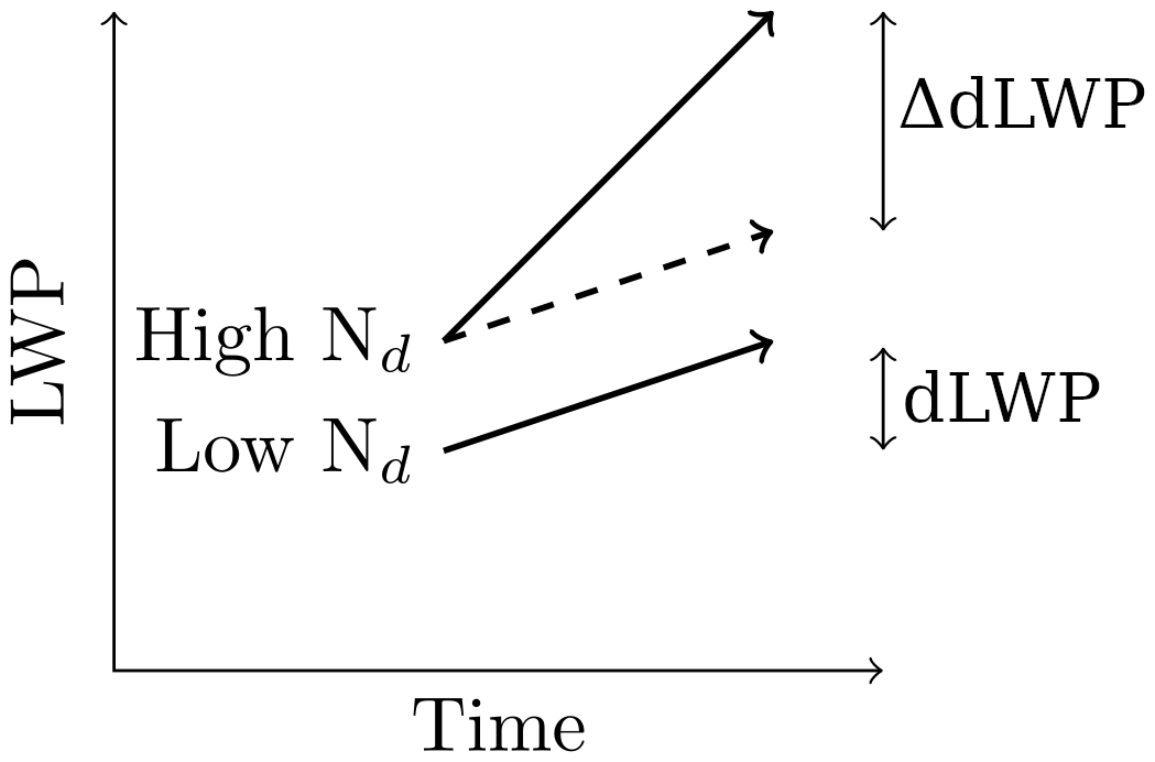
Figure 1 A schematic of the difference-in-differences method, showing how the N_d impact on LWP development is identified using the temporal development of the cloud field. This example shows a positive ΔdLWP. In Sect. 3.1 and 3.2, a threshold of 60 cm⁻³ is used to separate high and low N_d.

The difference in properties between the Aqua and Terra overpasses is indicated with a “d” in this context, i.e. dLWP is the afternoon (Aqua) LWP minus the morning (Terra) LWP. Separating the population of clouds into two groups (those with a starting N_d more and less than the median value of 60 cm⁻³), ${\mathrm{\Delta }}_{N_{\mathrm{d}}}$dLWP is defined as the difference in the dLWP for the above and below 60 cm⁻³ N_d groups. As the evolution in this work is always separated by the other variable, the subscript on the Δ is omitted.

A positive ΔdLWP means that the high N_d population gained more (or lost less) LWP over the 3 h period than the low N_d population. This would suggest a positive N_d impact on LWP (and hence a negative radiative effect for LWP adjustments). The N_d–LWP relationship is also characterised using the “sensitivity”, the slope of the linear regression between the two values in log–log space ($\frac{\mathrm{d}\ln \mathrm{LWP}}{\mathrm{d}\ln N_{\mathrm{d}}}$ Feingold, 2003). Similar difference-in-differences calculations are performed for the N_d evolution, using populations above and below 60 g m⁻² (ΔdN_d).

To account for motion in the cloud field, the field is advected using ERA5 reanalysis fields at 1000 hPa, with this level selected as it can accurately predict the locations of ship tracks given the location of individual ships, confirming it is suitable for calculating cloud advection over short timescales (Gryspeerdt et al., 2021). The expected motion over 3 h is often less than 1^∘, and so the advection step is calculated at a 0.25^∘ by 0.25^∘ resolution. Each of these quarter-degree grid boxes is advected following the ERA5 winds. The end locations of these trajectories are used to sample the Aqua data, and these re-sampled data are aggregated to 1^∘ by 1^∘ resolution for this analysis. Pixels with no cloud retrieval (either morning or afternoon) are removed from this analysis. This means that the results in this work consider only the development of in-cloud LWP, matching the decomposition of the forcing into N_d (Twomey), LWP and CF components in previous work (Bellouin et al., 2020).

The CCCM (CERES–CloudSat–CALIPSO–MODIS) combined product (Kato et al., 2010) is used to examine the role of precipitation on the LWP and N_d development. The CloudSat precipitation flag (Haynes et al., 2009) from CCCM is used to calculate the probability of precipitation as a function of LWP and N_d. To select the most accurate precipitation identification, only oceanic, liquid-phase data are used over the period 2007–2011 (inclusive) are used for the CCCM part of this work. Both liquid precipitation and drizzle are considered as precipitating for the purposes of this analysis. The fractal nature of precipitation means that the probability of precipitation (calculated at the CloudSat ray scale) would have to be corrected before being used for a comparison with global models, where the occurrence of precipitation is determined at a much larger scale (Stephens et al., 2010).

3 Results

3.1 LWP development

In many regions, ΔdLWP is positive (Fig. 2a), particularly away from the stratocumulus decks. This suggests an increase (or weaker decrease) in LWP at higher N_d. The ΔdLWP is larger at mid-latitudes and towards the west of the subtropical oceanic regions (where the environment is typically more unstable). This result, with higher LWPs in higher N_d cases, is in contrast to previous studies looking at large-scale statistics, which typically show a reduction in LWP as N_d increases (e.g. Michibata et al., 2016; Gryspeerdt et al., 2019; Possner et al., 2020).

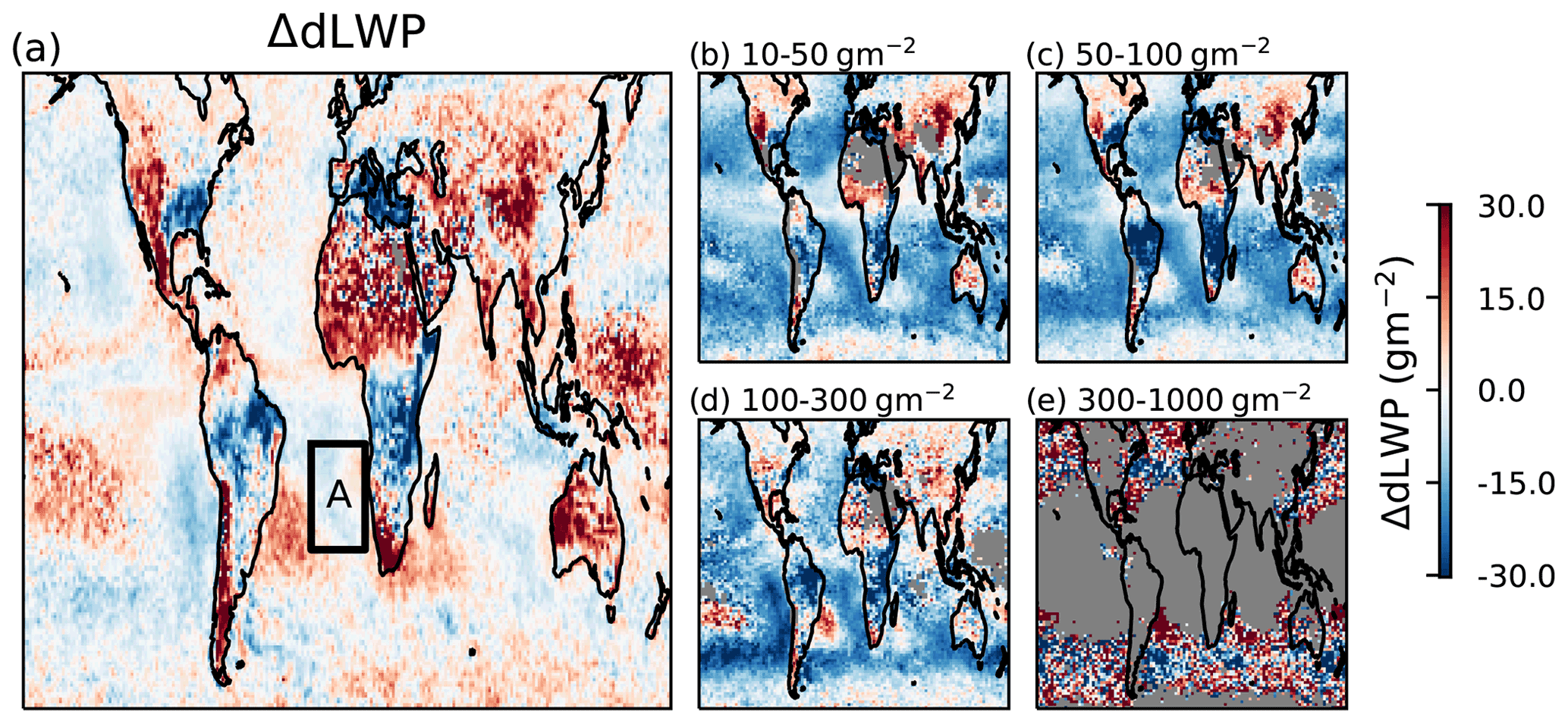
Figure 2 The difference in dLWP between high and low initial N_d populations (ΔdLWP). Red indicates a more positive dLWP for the high N_d population (N_d>60 cm⁻³). Panel (a) includes all available data, and panels (b–e) only consider cases where the initial LWP is within the specified bounds.

In this case, the positive ΔdLWP is an artefact of the strong initial negative N_d–LWP relationship, as observed in previous work (Han et al., 2002; Michibata et al., 2016; Gryspeerdt et al., 2019). Over the 3 h observation period, cases with a low initial LWP will tend to increase in LWP, whilst those with a high initial LWP will decrease (a concept known as regression to the mean), returning towards an LWP steady state (Hoffmann et al., 2020). This means that, on average, cases with a high initial N_d will have a low initial LWP and thus positive dLWP, producing the apparent positive N_d impact on LWP in Fig. 2a. This relationship appears whatever the driver of the initial N_d–LWP relationship. If the negative relationship is produced by a feedback (e.g. wet scavenging) rather than a N_d impact on LWP, it is possible to produce the observed apparent positive N_d impact on LWP even if N_d has no impact on LWP. By binning by the initial cloud state, this ensures that the high and low N_d populations start with the same LWP, removing the impact of this regression to the mean effect.

Controlling for the initial LWP uncovers a negative ΔdLWP in most regions and under most initial conditions, suggesting that an increase in N_d leads to a lower LWP over time (Fig. 2b–e). A positive ΔdLWP remains over land, particularly in cases with a low starting LWP. This might be related to convective invigoration (e.g. Koren et al., 2014), but the N_d retrieval is less accurate over land due to the lower adiabaticity of convective clouds (Gryspeerdt et al., 2022), leading to a low confidence in this result. The different apparent N_d impact on LWP highlights the importance of controlling for the initial cloud state when looking at cloud development.

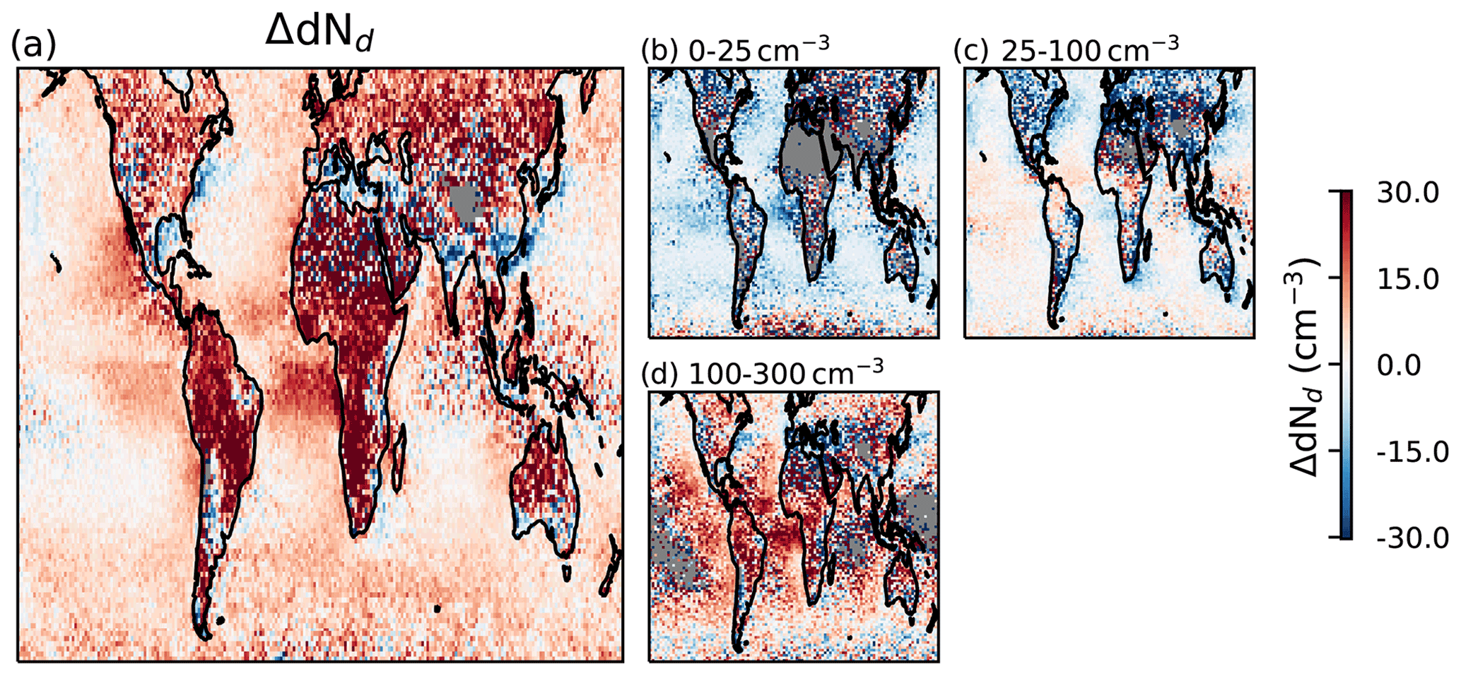
Figure 3 The same as Fig. 2 but showing the difference in N_d evolution between clouds with an initial LWP higher and lower than 60 g m⁻². Panel (a) shows all data, while panels (b–d) show cases where the initial N_d is restricted to the specified range. Note the larger fraction of missing data due to the more stringent sampling constraints on the N_d retrieval.

3.2 N_d development

Cloud and aerosol processes also modify the N_d over the 3 h period between the Terra and Aqua overpasses. Following Wood (2012), three processes are expected to dominate changes in N_d away from strong aerosol sources: CCN entrainment or dilution from mixing with the free troposphere, CCN production through sea salt emission, and the depletion of CCN through wet scavenging. Of these, wet scavenging is expected to have the strongest link to LWP, as precipitation is more common at high LWP (e.g. L'Ecuyer et al., 2009; Sorooshian et al., 2009) and thus produces a negative ΔdN_d. A positive ΔdN_d is instead found across most of the globe (Fig. 3a).

This positive ΔdN_d is strongest over land and in regions downwind of continents (e.g. the southeastern Atlantic Ocean, Sea of Japan and Tasman Sea; Fig. 3a) and is associated with pollution-dominated air masses in some locations (Fig. 3d).

In low initial N_d conditions (N_d<25 cm⁻³), a larger LWP results in a more negative ΔN_d. This is as expected from wet scavenging, where an increased LWP increases the probability of precipitation (e.g. Ludlam, 1951; Sorooshian et al., 2009; L'Ecuyer et al., 2009), reducing the N_d. In these cases, increasing the LWP increases the probability of precipitation, decreasing the N_d more strongly over time for higher initial LWP. This negative ΔdN_d is also visible near coastlines, particularly in the Northern Hemisphere, for moderate initial N_d cases (Fig. 3c). The regions of negative ΔdN_d in this case are typically in the more polluted locations. Positive ΔdN_d values are seen in the tropics.

In many polluted regions, particularly off the western coast of Africa, there are strong positive ΔdN_d values, which drive the overall ΔN_d response to LWP. This is the opposite of the impact expected from wet scavenging, as precipitation becomes relatively rare for N_d values above 100 cm⁻³, except at the largest LWPs (e.g. Fig. 5a–c). For the majority of both the high and the low LWP populations, the probability of precipitation is close to zero, obscuring the role of wet scavenging.

With precipitation uncommon, ΔdN_d at high N_d isolates the impacts of CCN entrainment and production in driving ΔdN_d. With free-troposphere CCN being a major CCN source (Wood et al., 2012), this increase in N_d at high LWP is likely due to the warm, moist air that often accompanies biomass burning aerosol (Adebiyi et al., 2015). When above the cloud, the moist smoke layer reduces cloud top cooling, limiting the LWP and providing no extra N_d. However, when the moist smoke layer is in contact with the cloud, LWP increases and the additional source of CCN gradually increases the N_d (Yamaguchi et al., 2015). This source effect is only visible in non-precipitating situations, as precipitation typically dominates the N_d budget in marine locations (Wood et al., 2012).

3.3 N_d–LWP development

The maps in Figs. 2 and 3 show a global variation in cloud development as a function of initial N_d and LWP but are a relatively coarse tool, hiding much of the complexity of the N_d–LWP temporal development. Figure 4 shows how the LWP and N_d change over 3 h (dLWP, dN_d) as a function of the initial LWP and N_d for a region within the southeastern Atlantic stratocumulus deck (region A in Fig. 2a).

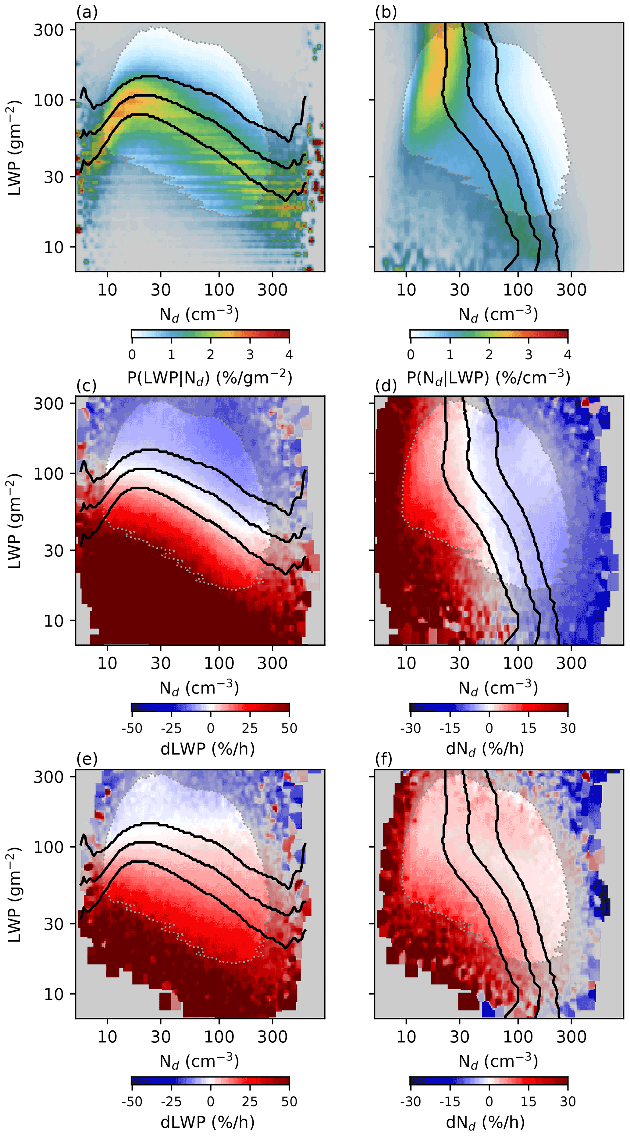
Figure 4 N_d–LWP development fields for Namibian stratocumulus region (A in Fig. 2a). (a) The probability of observing an initial LWP for a given initial N_d (P(LWP|N_d)) and (b) P(N_d|LWP). (c, d) Red is a positive (c) dLWP or (d) dN_d for a given initial (morning, Terra) N_d and LWP, while blue is negative (decrease in LWP or N_d). The fields are smoothed with a Gaussian window filter. Panels (e, f) are the same as (c, d) but are binned using the final (afternoon, Aqua) N_d and LWP. The black lines are at  the 25th, 50th and 75th percentiles. Regions with fewer than 30 retrievals per bin are shaded grey.

This region displays the “inverted-V” pattern for LWP as a function of initial N_d (Fig. 4a), with a positive slope at low N_d (consistent with precipitation suppression) and a negative slope at high N_d, consistent with increased entrainment at high N_d (Gryspeerdt et al., 2019). In contrast to this inverted-V pattern, the N_d normalised by LWP (Fig. 4b) shows a monotonic decrease in N_d as the LWP increases, becoming constant at high LWP.

The LWP evolution (Fig. 4c) reflects the initial LWP distribution in Fig. 4a. For a given N_d, positive dLWP is found at lower initial LWPs, and a negative dLWP is found at higher initial LWP. This relationship is also a clear function of the initial N_d, with the dLWP = 0 contour reducing as the initial N_d increases. The positive dLWP values at lower LWP are much stronger than the negative values found at high LWP. This overall pattern is very similar to that obtained from large eddy simulation (LES) modelling (Hoffmann et al., 2020). The strong dependence on dLWP on LWP highlights the importance of considering the initial LWP when investigating temporal LWP changes.

Similarly, the N_d evolution (Fig. 4d) reflects the N_d distribution in Fig. 4b. Positive dN_d values are found at low initial N_d, and negative values are found at high N_d. This means that the N_d would be expected to collapse over time to the dN_d=0 contour. The dN_d=0 contour is not in the same location as the peak of the N_d distribution in Fig. 4b, indicating that the N_d is not in equilibrium.

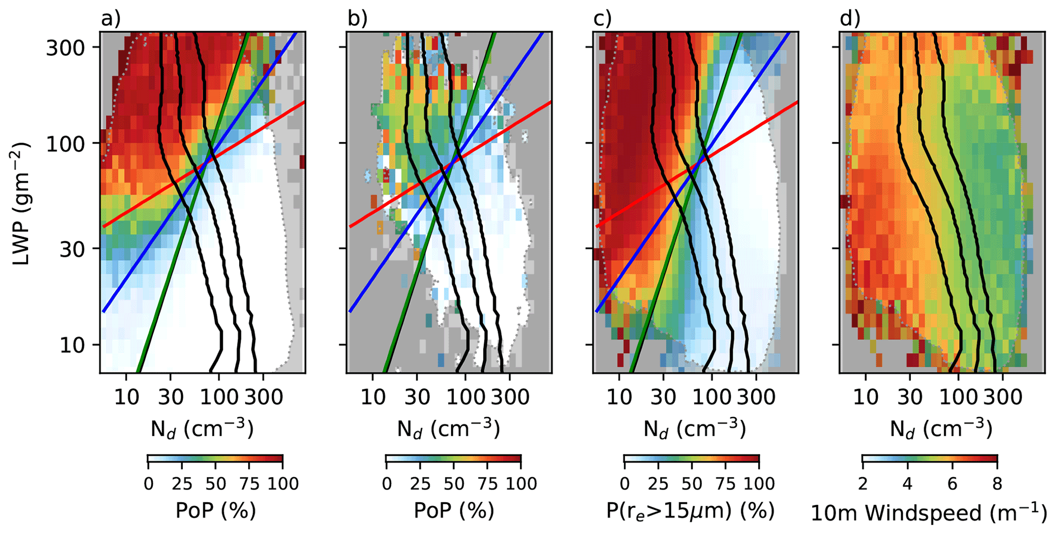
Figure 5 (a) The CloudSat probability of precipitation as a function of N_d and LWP at a pixel (1 km) resolution. The lines are contours of constant autoconversion rate from Tripoli and Cotton (1980, red), Liu and Daum (2004, blue), and Khairoutdinov and Kogan (2000, green). Panel (b) is the same as (a) but for N_d and LWP at a 1^∘ by 1^∘ resolution. (c) The proportion of liquid r_e retrievals >15 µm for N_d and LWP at a 1^∘ by 1^∘ resolution. (d) The average ERA5 wind speed as a function of LWP and N_d. Regions with fewer than 30 retrievals per bin are shaded grey.

The dLWP field (Fig. 4c) is similar to that found in model studies (Glassmeier et al., 2021), collapsing down to an approximate inverted-V shape, while the dN_d behaviour is quite different. In Glassmeier et al. (2021), dN_d is negative at low N_d (due to wet scavenging depleting N_d over time) and positive at high N_d (due to an aerosol source), causing the N_d to diverge over time. This is in contrast to the dN_d behaviour in Fig. 4d, where the N_d flow pattern converges towards an equilibrium value. Some of these differences may be explained by differences in the time of day (Glassmeier et al., 2021, was nocturnal, whereas these are daytime satellite retrievals), but meteorological controls on N_d may also play a role.

3.4 Meteorological controls on N_d development

The primary controls on N_d development are the production of CCN through sea salt and marine aerosol precursor emission (increasing N_d), wet scavenging (reducing N_d), and mixing with free-troposphere air (increasing or decreasing N_d; Wood, 2012). While modelling wet scavenging, Glassmeier et al. (2021) include a constant aerosol source, which does not depend on these environmental controls in the same way.

Sea salt production depends strongly on the local wind speed and is correlated to the N_d. This relationship is not linear. While wind speed (or sea salt production) are positively correlated with N_d at low wind speeds, decreases in N_d have been observed at high wind speeds and sea salt burdens, potentially due to the impact of giant CCN (Gryspeerdt et al., 2016; McCoy et al., 2018). This is reflected in Fig. 5d, where the highest wind speeds (and so positive impact on dN_d) are found at low N_d values, with little dependence on the LWP. Sea salt production therefore contributes to the positive dN_d, primarily at low N_d values, where the wind speed is strongest. Similar relationships are likely for the emission of marine aerosol precursors (such as dimethyl sulfide, DMS), which can make up a large fraction of the CCN at low wind speeds (Sanchez et al., 2018).

Free-troposphere mixing exchanges aerosol with a large reservoir, which has the effect of bringing the N_d back towards the free-troposphere value. At low N_d values, this produces a positive dN_d. At high N_d values, this produces a negative dN_d. Some correlation to LWP is possible, as the free-troposphere CCN can be correlated to the humidity, which is itself correlated to the LWP for underlying marine stratocumulus (e.g. Fig. 3d, Gryspeerdt et al., 2019). However, the dN_d produced by free-tropospheric mixing is largely independent of LWP (Fig. 4d).

The impact of wet scavenging is observed in the upper-left quadrant of Fig. 4d, but it does not dominate the dN_d. Following the dN_d=0 contour, at higher LWP values this contour shifts to lower N_d. However, wet scavenging is not strong enough to produce a negative dN_d across the precipitating region of Fig. 4d. This is due to the sub-grid variability in cloud properties at 1^∘ by 1^∘ resolutions.

When calculated at a pixel level, the probability of precipitation (PoP) is a strong function of both the LWP and N_d (Fig. 5a), with low-N_d, high-LWP cases having a PoP of over 80 %. At this resolution, the transition from precipitating to non-precipitating is sharp and close to linear in log–log space. Assuming an adiabatic liquid water content profile, the PoP edge is parallel to contours of the autoconversion rate from the Liu and Daum (2004) scheme. At a 1 km resolution, precipitation becomes rare as LWP drops below 30 g m⁻². The mean state N_d becomes relatively insensitive to LWP increases above this boundary (Figs. 4b and 5a, black lines), but a clear transition such as this might be expected produce a clear boundary in Fig. 4d along this edge. Although precipitation is important for N_d evolution, no clear transition in the N_d evolution is observed.

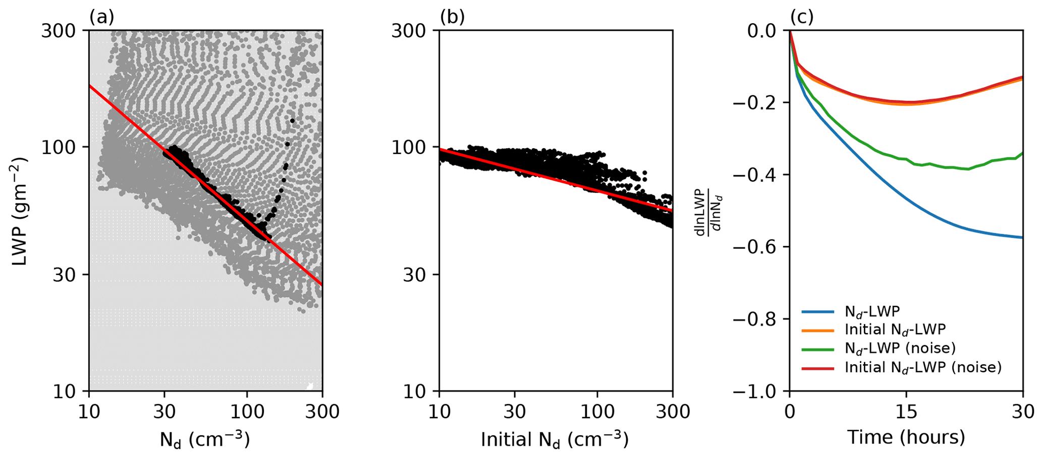
Figure 6 Temporal evolution of sensitivity assuming a constant flowfield for region A in Fig. 2a. (a) The instantaneous N_d–LWP relationship after 3 h (grey) and 24 h (black) from a distribution of points that have no initial N_d–LWP relationship (light grey). (b) The relationship between the initial N_d and LWP for the same data. (c) $\frac{\mathrm{d}\ln \mathrm{LWP}}{\mathrm{d}\ln N_{\mathrm{d}}}$ as a function of time measured using the instantaneous relationship (blue) and initial N_d (orange). Green and red are these relationships with Gaussian noise applied to the flowfield evolution. The red and orange lines overlap.

Precipitation is a non-linear function of N_d and LWP; sub-grid variability in cloud water and N_d modifies the autoconversion rate (Zhang et al., 2019). This is clear when calculating the PoP at 1^∘ by 1^∘ resolution (Fig. 5b). While the high-N_d, low-LWP cases are still primarily non-precipitating, the probability of precipitation for the low-N_d cases peaks at around 50 % (so only half of CloudSat rays in liquid cloud conditions are precipitating). Precipitation is even observed in cases with high N_d.

Similar variability is observed when using the cloud top effective radius (r_e) as a measure of precipitation (Fig. 5c). Using the probability of a 1 km pixel having an r_e>15 µm, a much stronger relationship between N_d and precipitation is observed at 1^∘ than at 1 km, with this transition being parallel to the Khairoutdinov and Kogan (2000) autoconversion rate. This transition is also less complete, with the probability of finding an r_e>15 µm not falling below a few percent. This sub-grid variability decreases the precipitation contrast between the precipitating and non-precipitating regions, obscuring the impact of wet scavenging in these results.

The lack of a clear dividing line into precipitating and non-precipitating regions in the N_d–LWP plot blurs the impact of wet scavenging, in contrast to high-resolution model simulations (Hoffmann et al., 2020). When combined with an aerosol source that is weakly dependent on N_d (the sea salt source) and free-troposphere entrainment that can act as an aerosol sink in high-N_d cases, this produces a N_d state that converges towards a stable state (Fig. 4d), rather than the diverging, unstable state seen in model studies (Glassmeier et al., 2021). This blurring effect also hides the second potential stable state at high N_d seen in previous model studies (Baker and Charlson, 1990). Although wet scavenging has a relatively subtle effect on the N_d flowfield in Fig. 4d, it still has a clear effect on the equilibrium N_d. As the LWP increases into the precipitating regime, the dN_d=0 contour shifts from around 60 to closer to 30 cm⁻³. This is consistent with the results of Wood (2012), who demonstrated the key role of wet scavenging in setting the mean N_d.

3.5 Implications for the LWP response to N_d

Combining the two development fields in Fig. 4c and d specifies the function ΔLWP, $\mathrm{\Delta }{N}_{\mathrm{d}}=f(\mathrm{LWP},N_{\mathrm{d}})$. This function is used to evolve a joint (N_d, LWP) distribution, producing an N_d–LWP slope and allowing these flowfields to be compared to previous studies that identified $\frac{\mathrm{d}\ln \mathrm{LWP}}{\mathrm{d}\ln N_{\mathrm{d}}}$ (Han et al., 2002; Michibata et al., 2016; Gryspeerdt et al., 2019). Although this makes the somewhat unrealistic assumption that the function remains constant with time, it allows for a comparison with previous studies of the instantaneous N_d–LWP relationship and provides a method to examine the impact of feedbacks in the system.

With an initial array of (LWP, N_d) points that are sampled so that there is no initial N_d–LWP relationship, these points are then stepped forward using the fields shown in Fig. 4. After eight steps (approximately 24 h), this produces the strong negative N_d–LWP relationship shown in Fig. 6a. The temporal development of the N_d–LWP sensitivity for this population is shown in Fig. 6c by the blue line, with the sensitivity reaching a minimum of −0.7 at around 15 h (five time steps). Similar to recent model studies (Glassmeier et al., 2021), this sensitivity is noticeably stronger than previous observational studies, which are typically smaller than −0.4 and closer to −0.1 (Toll et al., 2019; Gryspeerdt et al., 2019).

One complicating factor in measuring the N_d impact on LWP is that the N_d also evolves with time. This means that the measured sensitivity at each time step is the combination of N_d impacts on LWP and feedback processes that modify the N_d. As the N_d evolution also acts to create a negative N_d–LWP relationship, the instantaneous N_d–LWP relationship at a given time step is not a good measure of the causal N_d–LWP relationship. To minimise this issue, we also show the relationship between the initial N_d and the evolved LWP after 24 h (Fig. 6b). This shows a weaker sensitivity, with a minimum around 10–12 h before decreasing (absolute value) again with time (Fig. 6c, orange line). At −0.2 the peak sensitivity is less negative than the instantaneous N_d–LWP sensitivity (blue line), but it is still more negative than that obtained in many observational studies. This temporal development is due to the weaker LWP reduction in low-N_d cases (Fig. 4c). An approximately linear relationship is formed initially, before additional LWP reductions generate the weak N_d–LWP relationship below 30 cm⁻³, weakening the overall relationship (Fig. 6b).

A further complication comes from representing factors controlling the N_d and LWP evolution other than the current N_d and LWP state. Random errors in the retrievals, local variations in meteorological parameters or changes in the background aerosol properties may all have a role in the N_d and LWP evolution. If these other factors are uncorrelated to the current N_d and LWP, they can be represented as noise on the dLWP and dN_d terms. Adding noise to the (LWP, N_d) evolution weakens the instantaneous sensitivity (Fig. 6c, green line), primarily by widening the N_d range to include the non-linear regions at low and high N_d. The magnitude of the weakening effect depends strongly on the strength of the noise. As the measurements used in this work already contain a noise component, this might suggest that the sensitivities obtained in this work are too weak – a more accurate measure of the temporal evolution of clouds might produce stronger sensitivities.

3.6 The global distribution

The dLWP and dN_d fields in Fig. 4 and their evolution (as in Fig. 6) vary across the globe due to variations in the background meteorological state and aerosol properties, becoming positive in some regions. Figure 7a shows the average sensitivity for the period 18–24 h after the integration is started. The sensitivity is strongly negative over almost all ocean regions (consistent with Fig. 2), while a slight positive sensitivity is observed over land. The stratocumulus sensitivity is above −0.6 in many regions, which would lead to a complete cancellation of the forcing from the Twomey effect and a positive effective radiative forcing from aerosol–cloud interactions in these locations (Glassmeier et al., 2021).

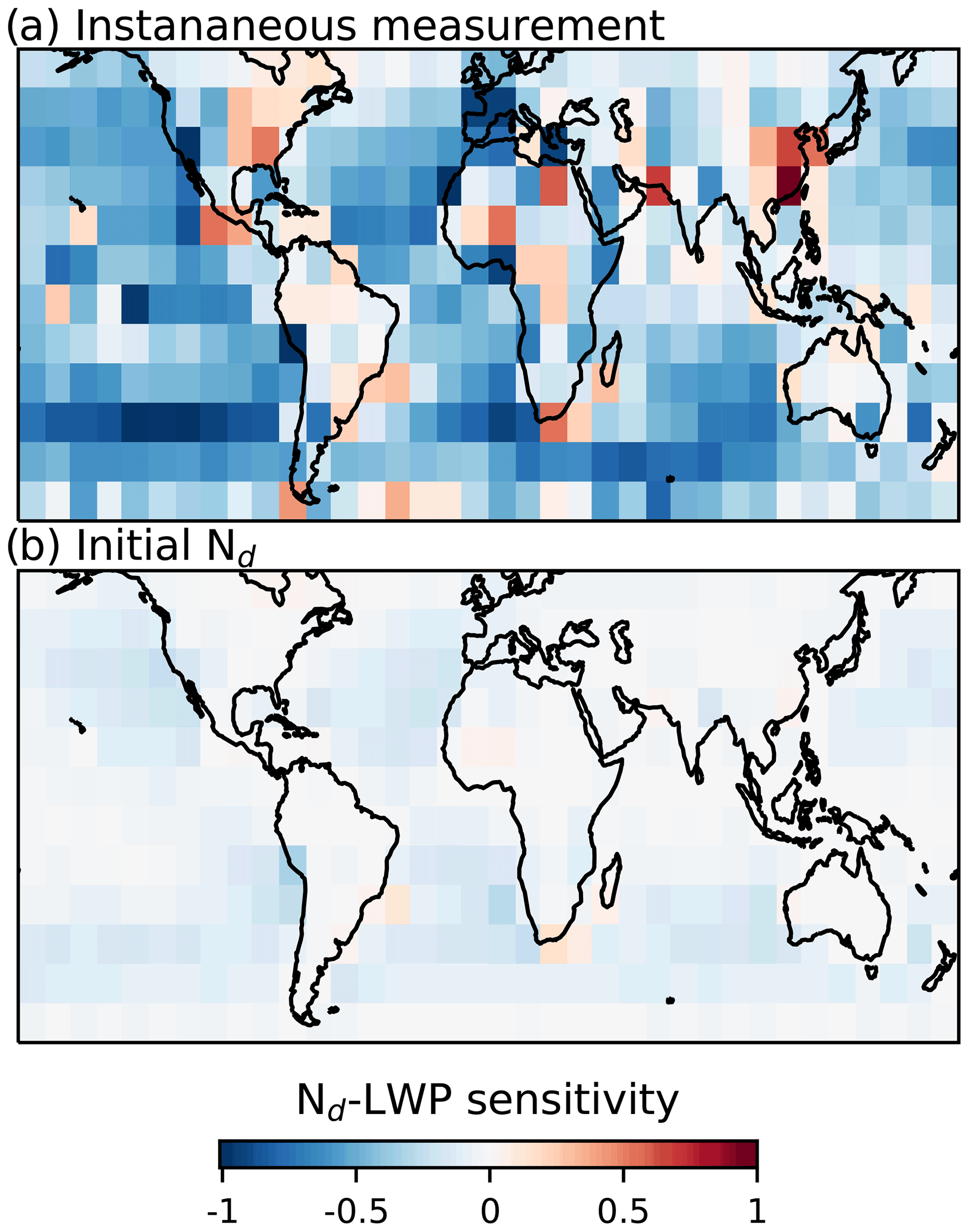
Figure 7 (a) The instantaneous sensitivity averaged over the period 18–24 h for each 10^∘ by 10^∘ area, and (b) the equivalent data using the initial N_d for calculating the sensitivity.

As noted in the previous section, the instantaneous sensitivity incorporates feedbacks on the N_d (such as wet scavenging) that act to steepen the N_d–LWP relationship. Figure 7b shows the N_d–LWP sensitivity calculated using the initial N_d, which is closer to the causal impact of N_d on LWP. There are many similarities between the spatial distributions, with more strongly negative sensitivities in the stratocumulus decks and positive sensitivities over land. These sensitivities support some previous conclusions, with negative sensitivities in stratocumulus regions (Toll et al., 2019) and a weak negative sensitivity downwind of Hawaii (Gryspeerdt et al., 2019). The overall magnitude of the sensitivity is much weaker, peaking close to −0.2 in the stratocumulus decks. This N_d–LWP sensitivity would offset around half of the Twomey effect, with a reduction in LWP and a positive radiative forcing stronger than that derived from ship tracks (Toll et al., 2019), but weaker than that derived from MODIS data alone (Gryspeerdt et al., 2019).

4 Discussion

While these results show that the short-term behaviour of the LWP and N_d is consistent with the impacts of wet scavenging, CCN production and free-troposphere mixing, some uncertainties in this work remain, particularly around the impact of retrieval uncertainties, the specification of the initial state for integration and the impact of factors that remain unaccounted for.

Systematic biases in retrievals have long been an issue with observation-based aerosol–cloud studies (e.g. Quaas et al., 2010). Studying the temporal development of a scene can reduce these biases, as they are the same for both the initial and final state and thus do not impact dLWP or dN_d (Fig. 1). However, temporal development is subject to a different class of biases created by random retrieval errors, namely regression to the mean. If a random error results in a high bias to the LWP, the later second retrieval is very likely to be smaller. This creates a negative dLWP at high LWP and a positive one at low LWP (and similar for N_d), biases which are not removed even by averaging over large datasets.

However, if regression to the mean were driving the results in this work (such as the flowfields in Fig. 4), the flowfields would look the same if they were calculated in either direction – that is binning dLWP and dN_d by the final LWP and N_d. Figure 4e and f shows the results of this backward flowfield, calculating dLWP and dN_d relative to the final LWP and N_d. The result is different to the forward flowfields in Fig. 4c and d. The dLWP = 0 line is at a much higher LWP for the backward flowfield when compared to the forward flowfield, with only a few negative values observed at very high LWPs. The difference in the dN_d field is even clearer, almost no negative dN_d values are observed. While this does not completely rule out the impact of retrieval biases and the regression to the mean effect, it builds confidence that these results are not just a statistical artefact caused by random biases in the LWP and N_d retrievals.

It is also not yet clear how best to use these flowfields to calculate a final sensitivity value. In this work, we assume that the flowfield is evenly populated and integrate it until a slope in the data becomes clear. Should all initial points in the flowfield be given equal weighting? How can this best be compared to more traditional calculations of the sensitivity? The inclusion of noise into the integrations also reduces the sensitivity obtained. What is the appropriate level of noise to include? Do the flowfields remain constant long enough for this technique to be valid? The analysis of short-term cloud development along trajectories using geostationary data provides one pathway to answering these questions and will be explored in future work.

5 Conclusions

The impact of correlated errors in N_d and LWP retrievals makes observed N_d–LWP relationships difficult to interpret. The response of LWP to aerosol perturbations (such as from ships or industry) provides one potential solution to this, but this is only applicable if time development is taken into account.

In this work, we look at the short-term development of LWP and N_d as a function of the initial state between overpasses of MODIS instruments (approximately 3 h). Controlling for the initial state reduces the impact of these correlated errors, showing that the LWP and N_d evolution is highly dependent on the initial state. The instantaneous N_d–LWP correlation is strong enough to generate spurious relationships between the N_d and LWP development if it is not accounted for (Fig. 2a), but once it is, there is clear evidence of a decrease in LWP at higher N_d levels (Fig. 2). A wet-scavenging effect, reducing N_d as LWP increases, is only visible under low-N_d conditions. In high-N_d environments, N_d tends to increase as the LWP increases, potentially due to a meteorological covariation between CCN sources and air mass properties (Fig. 3).

Binning these short-term changes in LWP and N_d as a function of the initial LWP and N_d can represent the cloud development in more detail (Fig. 4). Although these fields are unlikely to be constant in time, integrating them forward can convert these 3-hourly development values into a sensitivity suitable for comparing to previous work (Fig. 6). This produces a strongly negative N_d–LWP relationship similar to model studies (Glassmeier et al., 2021), although the evolution of the N_d complicates the interpretation of the N_d–LWP relationship. Using the initial N_d to calculate the N_d–LWP sensitivity accounts for these feedback processes, resulting in a weaker sensitivity of LWP to N_d variations. This sensitivity varies globally; although it is stronger in stratocumulus regions, it is still weaker than the sensitivity calculated using instantaneous MODIS data.

While this work demonstrates a potential method for accounting for feedbacks when evaluating the N_d–LWP relationship, it is still affected by potential retrieval biases in the N_d and LWP retrievals that could affect the quantification of the initial state. To accurately quantify the aerosol impact on LWP, variability in the N_d–LWP relationship would have to be accounted for. The diurnal cycle and local meteorological conditions have an impact on LWP evolution and N_d, likely affecting the results in Figs. 6c and 7). Geostationary satellites provide a natural pathway forward, although night-time retrievals of cloud properties are challenging. Future work should also account for the possibility that these relationships are not constant under warming (Zhang et al., 2022; Murray-Watson and Gryspeerdt, 2022).

Although the magnitude of the N_d–LWP relationship derived here is only indicative of the N_d impact on LWP, this work provides a pathway to make use of geostationary observations for constraining cloud processes. It also highlights that the instantaneous N_d–LWP relationship measured along a trajectory may not be a good measure of how the LWP is responding to N_d variations. It is vital that trajectory- and temporal-evolution-based studies have the same initial conditions if they are to successfully isolate the aerosol impact on cloud properties and development.