the Creative Commons Attribution 4.0 License.
the Creative Commons Attribution 4.0 License.
 | 09 Sep 2022
Updated trends of the stratospheric ozone vertical distribution in the 60° S–60° N latitude range based on the LOTUS regression model
Sophie Godin-Beekmann
Niramson Azouz
Viktoria F. Sofieva
Daan Hubert
Irina Petropavlovskikh
Peter Effertz
Gérard Ancellet
Doug A. Degenstein
Daniel Zawada
Lucien Froidevaux
Stacey Frith
Jeannette Wild
Sean Davis
Wolfgang Steinbrecht
Thierry Leblanc
Richard Querel
Kleareti Tourpali
Robert Damadeo
Eliane Maillard Barras
René Stübi
Corinne Vigouroux
Carlo Arosio
Gerald Nedoluha
Ian Boyd
Roeland Van Malderen
Emmanuel Mahieu
Dan Smale
Ralf Sussmann
This study presents an updated evaluation of stratospheric ozone profile trends in the 60∘ S–60∘ N latitude range over the 2000–2020 period using an updated version of the Long-term Ozone Trends and Uncertainties in the Stratosphere (LOTUS) regression model that was used to evaluate such trends up to 2016 for the last WMO Ozone Assessment (2018). In addition to the derivation of detailed trends as a function of latitude and vertical coordinates, the regressions are performed with the datasets averaged over broad latitude bands, i.e. 60–35∘ S, 20∘ S–20∘ N and 35–60∘ N. The same methodology as in the last assessment is applied to combine trends in these broad latitude bands in order to compare the results with the previous studies. Longitudinally resolved merged satellite records are also considered in order to provide a better comparison with trends retrieved from ground-based records, e.g. lidar, ozonesondes, Umkehr, microwave and Fourier transform infrared (FTIR) spectrometers at selected stations where long-term time series are available. The study includes a comparison with trends derived from the REF-C2 simulations of the Chemistry Climate Model Initiative (CCMI-1). This work confirms past results showing an ozone increase in the upper stratosphere, which is now significant in the three broad latitude bands. The increase is largest in the Northern and Southern Hemisphere midlatitudes, with ∼2.2 ± 0.7 % per decade at ∼2.1 hPa and ∼2.1 ± 0.6 % per decade at ∼3.2 hPa respectively compared to ∼1.6 ± 0.6 % per decade at ∼2.6 hPa in the tropics. New trend signals have emerged from the records, such as a significant decrease in ozone in the tropics around 35 hPa and a non-significant increase in ozone in the southern midlatitudes at about 20 hPa. Non-significant negative ozone trends are derived in the lowermost stratosphere, with the most pronounced trends in the tropics. While a very good agreement is obtained between trends from merged satellite records and the CCMI-1 REF-C2 simulation in the upper stratosphere, observed negative trends in the lower stratosphere are not reproduced by models at southern and, in particular, at northern midlatitudes, where models report an ozone increase. However, the lower-stratospheric trend uncertainties are quite large, for both measured and modelled trends. Finally, 2000–2020 stratospheric ozone trends derived from the ground-based and longitudinally resolved satellite records are in reasonable agreement over the European Alpine and tropical regions, while at the Lauder station in the Southern Hemisphere midlatitudes they show some differences.
- Article
(3349 KB) - Full-text XML
-
Supplement
(822 KB) - BibTeX
- EndNote


The recovery of the ozone layer has been under scrutiny since the peak of ozone-depleting substances (ODSs) was reached in the stratosphere in the middle and end of the 1990s depending on the latitude region (e.g. Newman et al., 2007) in response to reduced ODS emissions imposed by the 1987 Montreal Protocol and its subsequent amendments. After first indications of a small ozone increase from various ground-based and satellite records in the upper stratosphere, i.e. above ∼35 km (WMO, 2010), clear evidence of the impact of decreasing ODS content on ozone levels in that altitude region was provided in WMO (2014) and references therein. Since then, an upper-stratospheric ozone increase has been confirmed by various studies (e.g. Harris et al., 2015; Steinbrecht et al., 2017; Petropavlovskikh et al., 2019). In parallel, chemistry climate models (CCMs) have attributed half of this increase to decreased ODS concentrations and half to upper-stratospheric cooling resulting from increased greenhouse gases (GHGs), which slows gas-phase ozone-depleting reactions (e.g. chap. 5 of WMO, 2018). In contrast, an ozone increase in the lower stratosphere has not been detected to date, except for some emerging signs in the Antarctic polar region in spring (de Laat et al., 2015; Solomon et al., 2016; Pazmiño et al., 2018; WMO, 2018).
The issue of ozone evolution and recovery in the lower stratosphere has received a lot of attention in recent years. Using several long-term satellite combined records and derived trends based on the dynamical linear modelling (DLM) method, Ball et al. (2018) found a decline in ozone in the lower stratosphere over the period 1998–2016. This result was challenged by Chipperfield et al. (2018), who argued that the ozone reduction was influenced by short-term dynamical variability at the end of the studied period. The cause for ozone decline or lack of recovery in the lower stratosphere was investigated by several model-based studies. Orbe et al. (2020) suggested that the observed decrease in ozone in the Northern Hemisphere could be explained by a poleward expansion of tropical upwelling and a reduced downwelling in the northern subtropical region. Other studies (Wargan et al., 2018; Ball et al., 2020) pointed to an enhanced meridional mixing between the tropics and the midlatitudes.
The present study is a follow-up of the ozone profile trend analysis performed within the LOTUS activity of the Stratosphere-troposphere Processes And their Role in Climate (SPARC) programme (Petropavlovskikh et al., 2019) that contributed to chap. 3 of the last WMO/UNEP Ozone Assessment (WMO, 2018) and is referred to as LOTUS19 hereafter. In order to achieve a consistent interpretation of stratospheric ozone changes, multiple merged satellite and ground-based data records of ozone vertical distribution were collected to perform the same trend analyses. Previously published multiple linear regression (MLR) models were tested on a common ozone dataset to evaluate the sensitivity of derived trends to the use of different models for the regression. This enabled the selection of the open-source LOTUS regression model (https://arg.usask.ca/docs/LOTUS_regression last access: 15 March 2022), maintained by the University of Saskatchewan. The trends in the vertical distribution of stratospheric ozone profiles were assessed over the period 1985–2016. A new approach was established for combining the trend estimates from individual satellite-based records into a single best estimate of ozone profile trends representative of the three broad latitude bands: 35–60∘ at Southern (SH) and Northern Hemisphere (NH) midlatitudes and 20∘ N–20∘ S in the tropics. Special attention was given to the evaluation of trend significance as a function of altitude. The LOTUS19 trend results were compared to those derived from previous studies (e.g. Harris et al., 2015; Steinbrecht et al., 2017). LOTUS19 found positive trends in the upper stratosphere in the post-ODS peak period (2000–2016) for both satellite and ground-based records. Results from merged satellite records showed statistically significant positive combined trends of 2 %–3 % per decade in the Northern Hemisphere midlatitudes in the ∼5–1 hPa pressure range and of 1 %–1.5 % per decade in the tropics in the ∼3–1 hPa pressure range. Combined trends were not statistically significant in the upper stratosphere at southern midlatitudes and no significant trends were obtained in the lower stratosphere. The LOTUS19-derived trends in broad latitude bands were also compared to trends from the Chemistry Climate Model Initiative (CCMI-1) simulations. Both models and merged satellite records showed similar results in terms of trend values and significance, except at southern midlatitudes in the upper stratosphere, where model trends were found to be significant.
Since LOTUS19, other studies assessed global stratospheric ozone profile trends. Szeląg et al. (2020) analysed the seasonal dependence of stratospheric ozone trends from four merged satellite datasets over the 2000–2018 period using a two-step MLR model. They found positive trends in the upper stratosphere at middle and high latitudes, maximizing during the winter. This is consistent with findings that due to GHG concentration increases, the Brewer–Dobson circulation, which is most effective in the winter season, should strengthen and accelerate the ozone recovery (e.g. Garcia and Randel, 2008). In the lower and middle stratosphere, negative trends were found in the tropics during all seasons, along with trends of varying sign depending on the season in the northern and southern midlatitudes. Another study by Sofieva et al. (2021) evaluated regional trends from the new MErged GRIdded Dataset of Ozone Profiles (MEGRIDOP) that combines ozone profile data from six limb-viewing satellite instruments. Zonal trend estimates agreed with previously published results. Longitudinally resolved trends showed a zonal asymmetry in the upper stratosphere at high and middle latitudes in the Northern Hemisphere with larger trends over Scandinavia than over Siberia.
In the present study, we compute trends from updated versions of the merged satellite records used in LOTUS19 and extended to the end of 2020, from the newly available MEGRIDOP merged time series and from updated versions of the ground-based data records selected from selected stations of the Network for the Detection of Atmospheric Composition Changes (NDACC), where observations of ozone profile as well as of other parameters are collected using a variety of ground-based techniques. Trends in the ozone vertical distribution derived from the various satellite and ground-based records as well as from CCMI-1 simulations considered in the study are evaluated using an updated version (version 0.8.0) of the LOTUS regression model.
The paper is organized as follows. Section 2 summarizes the satellite and ground-based records used in the study, while Sect. 3 describes the updated version of the LOTUS regression model that was employed to retrieve trends from the various records. Section 4 displays the different trend results for the merged satellite datasets both as a function of latitude and vertical levels and combined in broad latitude bands. Comparison between combined trends in broad latitude bands with corresponding LOTUS19 results and with trends computed from the updated CCMI-1 simulations are presented. In addition, trends from ground-based records at selected NDACC sites are compared to those from longitudinally resolved satellite data. Section 5 discusses improvements in trend retrievals with respect to LOTUS19, while conclusions of the study regarding long-term ozone profile changes are given in Sect. 6.
This section provides a brief description of the long-term ozone records used for trend retrieval. Readers can refer to Petropavlovskikh et al. (2019) for a more in-depth description of the various observational datasets (chap. 1 of the report).
2.1 Merged satellite records
Seven merged satellite records that were extended to December 2020 are used for this study (see also Table 2.2 of LOTUS19). The Global OZone Chemistry And Related trace gas Data records for the Stratosphere (GOZCARDS v.2.20) ozone monthly mean record includes the HALogen Occultation Experiment (HALOE; v19), Aura Microwave Limb Sounder (MLS v4.2), SAGE I (version 5.9) and SAGE II (v7) and covers the period 1979–2020. HALOE and Aura MLS measurements are adjusted with SAGE II data, which are used as a reference in the overlapping time periods (Froidevaux et al., 2015).
Data included in the Stratospheric Water and OzOne Satellite Homogenized (SWOOSH) merged record are Aura MLS v4.2, UARS MLS v5, UARS HALOE v19, SAGE II v7 and SAGE III v4. The merged records are homogenized to minimize artificial discontinuities and to account for inter-satellite biases in the record (Davis et al., 2016).
The Solar Backscatter Ultraviolet Merged total and profile Ozone Data (SBUV MOD) record includes data from the SBUV predominantly on the NOAA satellite series of instruments and the Ozone Mapping and Profiler Suite – Nadir Profiler (OMPS-NP) on the Suomi National Polar-orbiting Partnership (SNPP). Data from all SBUV instruments except the NOAA-9 instrument and the morning portion of NOAA-14 and NOAA-16 are included, providing a continuous coverage of ozone profiles since 1978. For the merged dataset, no external calibration adjustments are applied, as in-instrument calibration adjustments have already been applied at the radiance level within the retrieval algorithm. Measurements are averaged during periods when more than one instrument is operational (Frith et al., 2017). Version 8.7 of SBUV MOD is used in this study, which includes refined in-instrument calibration adjustments (for NOAA-16 through OMPS NP, using NOAA-19 as a reference) and a diurnal correction to account for varying measurement times (Frith et al., 2020).
Another approach was adopted for the SBUV Cohesive (SBUV COH) merged dataset that uses much of the same SBUV and OMPS instruments as SBUV MOD but retains the use of Version 8.6 for SBUV processing as in LOTUS19. The COH approach identifies a representative satellite for each time period and examines data for each overlapping period to improve the consistency of some satellite records with their neighbours. As in LOTUS19, the updated SBUV COH dataset used in this study adjusts NOAA-16, NOAA-17 and NOAA-19 to the NOAA-18 SBUV record, and also extends the record to 2020 with OMPS-NP from SNPP (NOAA v3r2 from NOAA/NESDIS), also adjusted to NOAA-18. Early data are minimally adjusted. Nimbus-7 and NOAA-11 are not adjusted, and NOAA-9 is used for a minimal time period to fill a data gap and is adjusted to NOAA-11 (Wild et al., 2019). SBUV COH uses Version 8.6 for SBUV data and the NOAA v3r2 version of the OMPS-NP retrieval.
The merged SAGE-CCI-OMPS dataset was developed in the framework of the European Space Agency Climate Change Initiative for Ozone (Ozone-CCI). It includes data from SAGE II, several ozone measuring instruments on board the Environmental Satellite (EnviSat), OSIRIS on Odin, ACE-FTS on the SCIence SATellite (SCISAT), and the OMPS – Limb Profiler (OMPS-LP) (Sofieva et al., 2017). The merging method consists in merging long-term deseasonalized anomalies from the individual satellite ozone records. A similar methodology has been used for the merged SAGE-OSIRIS-OMPS time series that includes data from SAGE II, OSIRIS and OMPS-LP Usask 2D records (Bourassa et al., 2018; Zawada et al., 2018).
Finally, the SAGE-SCIAMACHY-OMPS record includes data from SAGE II, the SCanning Imaging Absorption spectroMeter for Atmospheric CHartographY (SCIAMACHY) and OMPS-LP retrieved with University of Bremen code. The merging of SCIAMACHY and OMPS-LP records with SAGE II occultation observations is carried out from zonally averaged monthly anomalies (Arosio et al., 2019).
Compared to LOTUS19, the SAGE-MIPAS-OMPS record that was not extended to 2020 has been replaced by the SAGE-SCIAMACHY-OMPS record. Most other records were extended to 2020 with no substantial version change. SBUV MOD now includes OMPS-NP and uses the Version 8.7 retrieval algorithm for all datasets used. SBUV-COH is the same dataset as used in LOTUS19 through 2010. The NOAA-19 component for 2011 to 2013 has been reprocessed since the LOTUS19 report with enhanced calibrations but no algorithm change, and OMPS-NPP extends the data from 2014 to 2020. For better comparison with ground-based datasets, we also use the new MErged GRIdded Dataset of Ozone Profiles (MEGRIDOP) record (Sofieva et al., 2021). This dataset has a resolved longitudinal structure and is derived by merging six limb and occultation satellite datasets (GOMOS, SCIAMACHY and MIPAS on Envisat, OSIRIS, OMPS-LP, and Aura MLS), using a similar methodology as for SAGE-CCI-OMPS (Sofieva et al., 2021).
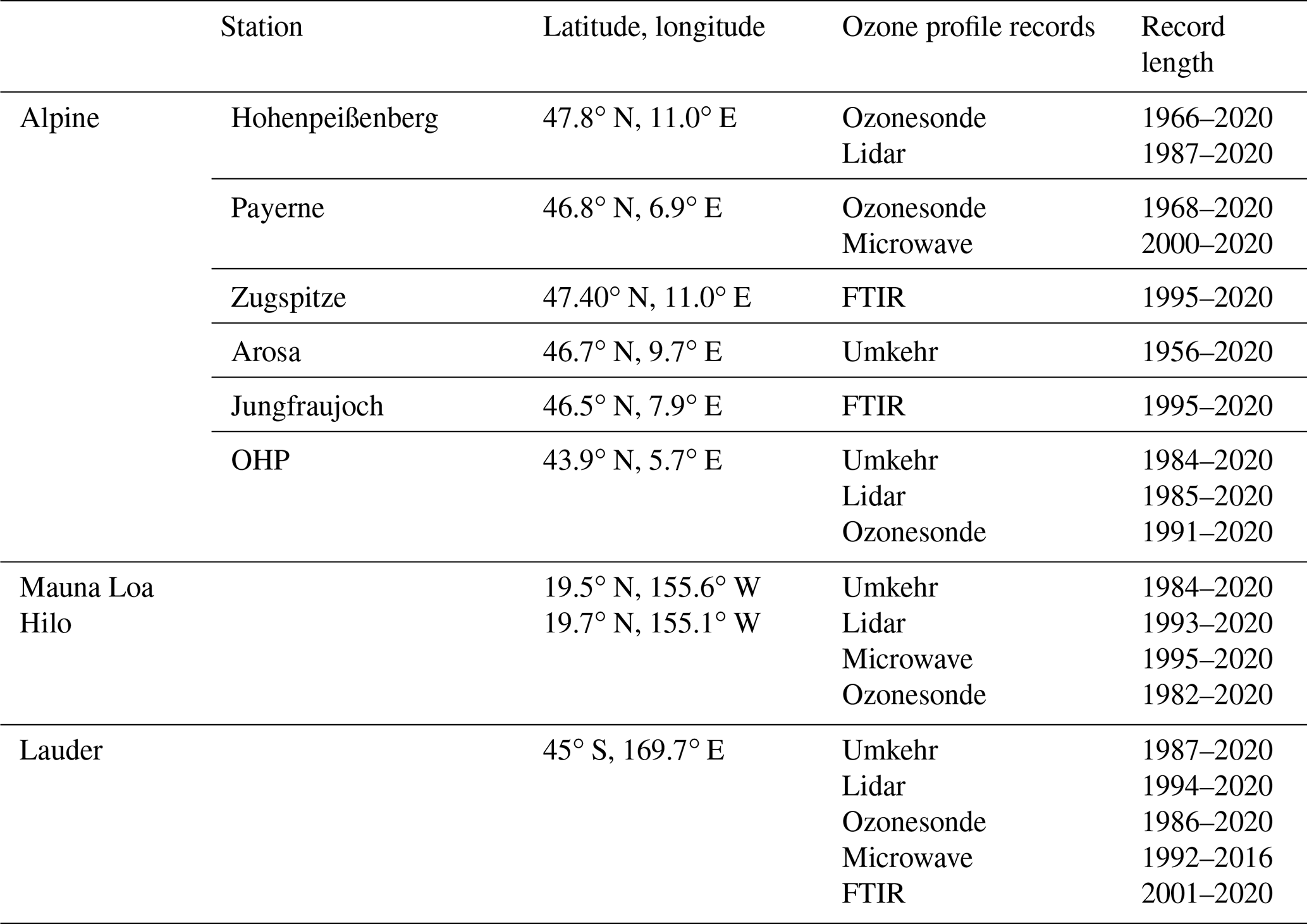
Table 1Long-term ground-based NDACC ozone profile records used in the study.
2.2 Ground-based records
Several NDACC stations were selected for trend comparison with merged satellite records. These stations provide multiple ground-based long-term ozone records using different techniques as mandated by the NDACC strategy (see also http://ndaccdemo.org/stations, last access: 15 April 2022). Ground-based measurement techniques used for the comparison include balloon-borne ozonesondes, lidar (light detection and ranging), microwave radiometer, Fourier transform infrared (FTIR) spectrometer and Umkehr profile retrieval from Dobson sunrise and sunset measurements. Ozonesondes are small balloon-borne instruments attached to a standard radiosonde. Based on an electrochemical sensing solution, they measure the ozone in situ profile from the ground to about 30–35 km altitude with a ∼150 m vertical resolution linked to balloon ascent rate and ozone cell response time. There are several types of ozonesondes and two of them are used in this study: the electrochemical concentration cell (ECC) and Brewer–Mast (BM). Each ozonesonde is a unique instrument and biases have been found in ozonesonde records linked to the preparation method, the type of sonde or the sensing solution used, or even to the batch of instruments purchased from manufacturers. Since 2004, the WMO/GAW-sponsored Assessment of Standard Operating Procedures of Ozonesondes (ASOPOS) panel has evaluated and intercompared ozonesonde measurements in the field or in laboratory chambers. The latest ASOPOS2 report (Smit, Thompson et al., 2021) provides recommendations on sonde preparation steps and measurement protocols, with the objective, by the adoption of these guidelines, of achieving the 5 % uncertainty level in tropospheric and stratospheric ozone requested by satellite and trend communities. Based on ASOPOS recommendations, ECC ozonesondes measurements records have been homogenized in multiple stations worldwide and the ECC ozonesonde data used in this study are from the Harmonization and Evaluation of Ground Based Instruments for Free Tropospheric Ozone Measurements (HEGIFTOM) prepared set of homogenized ozonesonde records.
Lidar is an active remote-sensing technique. For the measurement of the ozone vertical distribution it uses the emission of two laser wavelengths with different ozone absorption cross-sections according to the so-called differential absorption lidar (DIAL) technique. Pulsed lasers are used in order to obtain range-resolved measurements (e.g. Godin-Beekmann et al., 2003; Leblanc et al., 2016). This study uses lidar ozone profile records extended to 2020.
Microwave ozone radiometers (MWRs) detect emission spectra in the millimetre range produced by thermally excited rotational ozone transitions (e.g. Maillard Barras et al., 2020). The ozone profile retrieval is based on the pressure broadening effect of the emitted line with the use of the optimal estimation method (Rodgers et al., 2000; Bernet et al., 2019).
Umkehr ozone profiles are retrieved from the difference in zenith sky intensities selected from two spectral regions in the so-called C pair at 311.5 and 332.4 nm of Dobson and Brewer spectrometer measurements. The long-term record of Umkehr measurements from four NOAA Dobson spectrophotometers located at the Boulder, Observatoire de Haute-Provence (OHP), Mauna Loa (MLO) and Lauder stations has recently been reprocessed with the optimized homogenization technique (Petropavlovskikh et al., 2022), and the three latter improved records are used here.
The FTIR ozone measurements are performed over the 600–4500 cm−1 spectral range, with high-resolution spectrometers, using the sun as a source of light under clear-sky conditions. On top of total ozone columns, low vertical-resolution ozone profiles can be derived from the temperature and pressure dependence of the line shapes (Hase et al., 1999; Vigouroux et al., 2015). Table 1 summarizes the ground-based measurements performed in the selected NDACC stations and the length of the record.
The selected NDACC stations are Mauna Loa (MLO, lidar, microwave, Umkehr) and Hilo (for ozonesondes) in the tropics, Lauder in the Southern Hemisphere midlatitudes (lidar, ozonesondes, FTIR, Umkehr), and stations located in the vicinity of the European Alps in the Northern Hemisphere midlatitudes. These Alpine stations are Hohenpeißenberg (lidar, ozonesondes), Arosa (Umkehr), Payerne (microwave, ozonesondes), Zugspitze (FTIR), Jungfraujoch (FTIR) and the Observatoire de Haute-Provence (lidar, ozonesondes, Umkehr). The location of these stations within a radius of less than 700 km corresponds to one grid cell of the longitudinally resolved satellite records used in this study, i.e. 10∘ lat × 20∘ long for MEGRIDOP and 10∘ lat × 30∘ long for SBUV-MOD and SWOOSH, which facilitates the satellite–ground-based trend comparison.
2.3 CCMI-1 model data
In addition, we have used data from the chemistry–climate models (CCMs) participating in phase 1 of the Chemistry–Climate Model Initiative (CCMI-1; Eyring et al., 2013), which are able to capture the coupling between stratosphere and troposphere in terms of composition and physical climate processes more consistently than previous model generations. The REF-C2 simulation, which is a seamless simulation running from 1960 to 2100, was selected and the trend analysis was made over the period 1979–2020. REF-C2 experiments follow the WMO (2011) A1 scenario for ozone-depleting substances and the RCP6.0 for other greenhouse gases, tropospheric ozone precursors, and aerosol and aerosol precursor emissions. Ocean conditions are either modelled (from a separate climate model simulation) or internally generated (in the case of ocean-coupled models). The simulation includes state-of-knowledge historic forcings, with recommendations that the 11-year solar cycle and quasi-biennial oscillation (QBO) forcings be either internally model-generated or nudged from the dataset provided by the Free University of Berlin. No volcanic forcing was used in this reference simulation. For a detailed description of all forcings used in the reference simulations, see Eyring et al. (2013), Hegglin et al. (2016) and Morgenstern et al. (2017). For the CCMI-1 trend analysis, all necessary proxies were calculated directly from the relevant individual model simulations. We calculated the appropriate QBO and El Niño–Southern Oscillation (ENSO) proxies from the model data (zonal winds and sea surface temperatures, SSTs), and used the external forcings (e.g. 11-year solar cycle) as provided to the modelling groups taking into account their implementation. We note that although the recommendation for the REF-C2 set of simulations did not include volcanic forcing, we found that some models did use it. Moreover, as volcanic effects could appear via different routes (e.g. SSTs or QBO), stratospheric aerosol optical depth (sAOD) was used as a proxy in the trend analysis as forcing provided to the modelling groups; see Sect. 4.5.2 of the LOTUS19 report for an in-depth explanation of CCMI-1 trends calculation.
An updated version of the LOTUS regression model (version 0.8.0) is used for the trend computation. It relies on the classical multiple linear regression method, which estimates the variability of time series from explanatory variables from the general least squares approach. The explanatory variables or proxies used in the LOTUS model are the quasi-biennial oscillation (QBO), the El Niño–Southern Oscillation (ENSO), the 11-year solar cycle, the stratospheric aerosol optical depth (sAOD) and a long-term trend. As in LOTUS19, we use independent linear trend (ILT) terms to evaluate long-term changes before and after the ODS peak, i.e. before January 1997 and after January 2000. The LOTUS model is applied to the ozone records without weight based on, e.g., measurement uncertainty. Most datasets are provided as monthly mean time series and are deseasonalized within the LOTUS model using Fourier components representing annual and semi-annual variations. The fitting of the deseasonalized times series is based on the following equation:
y(z,t) is the monthly mean ozone anomaly time series at altitude z, are the fitted coefficients and ε(z,t) represents the residual term. QBO1 and QBO2 are two orthogonal components of the QBO calculated with principal component analysis. No lag is applied to the ENSO, sAOD and Solar F10.7 proxies. Data sources of these proxies are provided in Table 2. Regarding the trend terms, Lpre(t), Lpost(t) and Gap(t) are written as follows:
t1 corresponds to 1 January 1997 and t2 to 1 January 2000.
Table 2Sources of explanatory variables and proxy time series used in the LOTUS regression model.
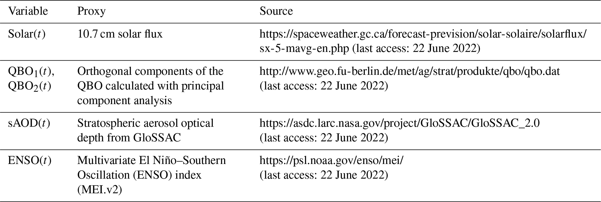
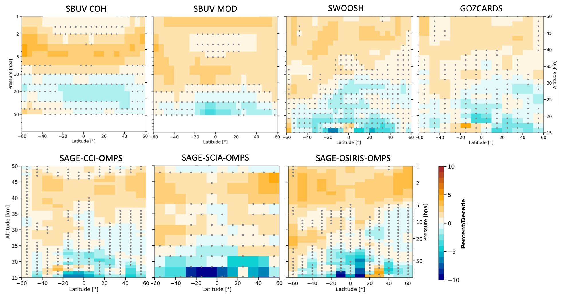
Figure 1Ozone profile trends from merged satellite records in percent per decade for the post-2000 period (January 2000–December 2020). Grey stippling denotes results that are not significantly different from zero at the 2σ level. Data are presented on their native latitudinal grid and vertical coordinate.
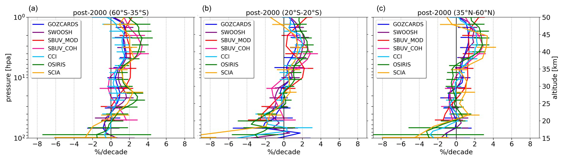
Figure 2Merged satellite ozone trends with their 2σ uncertainties for the post-2000 period as estimated by the LOTUS regression model for latitude bands 60–35∘ S (a), 20∘ S–20∘ N (b) and 35–60∘ N (c). Coloured lines are the trend estimates from the individual merged datasets on their native vertical grid.
The Cochrane and Orcut (1949) method is applied to correct for autocorrelation of residuals. Several improvements were made to the LOTUS model used in this work compared to the version used in LOTUS19. The new version (v0.8.0) of the model includes a seasonal variation of the regressed coefficient βk(z,t) for the various predictors, by adding Fourier components in the model as follows:
The new v0.8.0 LOTUS model also includes a new stratospheric aerosol optical depth (sAOD) predictor from the Global Satellite-based Stratospheric Aerosol Climatology (GloSSAC) instead of the NASA Goddard Institute for Space Science (GISS) sAOD used before. For detailed information on the LOTUS regression model and its new features since LOTUS19, see http://argpages.usask.ca/docs/LOTUS_regression/index.html (last access: 15 April 2022).
The improved LOTUS model with seasonal variation of fitted coefficients was applied to the merged satellite records included in the study over the 1985–2020 period for all latitude bins and altitude/pressure levels (depending on the native coordinates of the time series). It was also applied to each vertical level of the ground-based data used for comparison at the selected NDACC stations and to the gridded satellite data (e.g. MEGRIDOP, SWOOSH and SBUV MOD) in the vicinity of the stations. Trends from CCMI-1 model data were obtained from the updated v.0.8.0 LOTUS model in the same way.
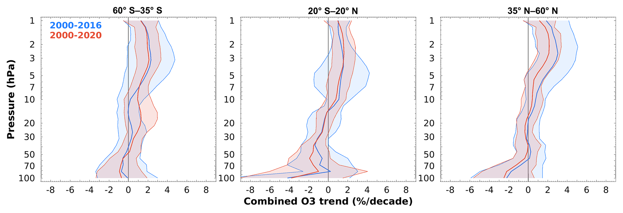
Figure 3Combined post-2000 ozone profile trend estimates and uncertainties (2σ) from the seven merged satellite records (below the 50 hPa level: five records, see text) for latitude bands 60–35∘ S (a), 20∘ S–20∘ N (b) and 35–60∘ N (c) as for Fig. 2. Red (blue) solid line and light red (blue) shaded areas indicate LOTUS22 (LOTUS19) trend values and uncertainties.
4.1 Global trends as a function of altitude/pressure and latitude from merged satellite records
Figure 1 displays the trend results for the post-2000 period (i.e. from 01/2000 to 12/2020) retrieved from the merged satellite records for all latitude bands and vertical bins. The upper row shows trend results for the merged satellite records provided in pressure levels (i.e. SBUV MOD, SBUV COH, GOZCARDS and SWOOSH), while trends from SAGE-CCI-OMPS, SAGE-SCIAMACHY-OMPS and SAGE-OSIRIS-OMPS provided in altitude levels are displayed in the bottom row. Dotted areas indicate trend values that are not significant at 2σ uncertainty. As in LOTUS19 (e.g. Fig. 5.2 of the report), positive and significant trend values are observed in the upper stratosphere for all datasets. Some discrepancies in the magnitude and latitude of the significant positive trends can be noticed among the records. In the upper row, the SBUV MOD record shows the largest positive trend values around 8 hPa and above 2 hPa, while positive trends of the other records are observed above 7–5 hPa and are generally significant for all latitude bands. Both SBUV MOD and SBUV COH display non-significant trends in the tropical and subtropical latitudes (above 2 hPa in the SBUV COH case). SWOOSH and GOZCARDS, which share similar individual satellite records, show similar trend patterns, with SWOOSH trend values slightly larger at 5 hPa in the midlatitudes. For records in the bottom row, the various trends are also very similar in the upper stratosphere, with increasing trend values from left to right panels. It is also interesting to see significant positive trend values for most records except SBUV COH in the southern midlatitudes in the middle stratosphere (above ∼25 km), while positive trends are not observed in this region in the Northern Hemisphere. In the lower stratosphere, trend values are generally negative but not significant, except in the lowermost stratosphere in the tropics and especially in the bottom row. These results are close to those of LOTUS19. The main feature of the zonally resolved trends is that most combined satellite records now show significant positive trends in vertical levels between ∼5–2 hPa for all latitude bands. This was not the case in LOTUS19 where trends from, e.g., GOZCARDS, SWOOSH and SAGE-CCI-OMPS were not statistically significant in the tropics.
4.2 Trends over broad latitude bands
As in previous ozone profile trend studies, e.g. Harris et al. (2015), Steinbrecht et al. (2017) and LOTUS19, we also calculated trends over broad latitude bands, namely 60–35∘ S, 20∘ S–20∘ N and 35–60∘ N. For GOZCARDS, SWOOSH, SBUV MOD and SBUV COH, we first computed the deseasonalized monthly anomalies with respect to their own 1998–2008 climatology for each latitude and pressure bin and then averaged these anomalies over the broad latitude band with latitude weights, in a similar way as in LOTUS19. The SAGE-SCIA-OMPS, SAGE-CCI-OMPS and SAGE-OSIRIS-OMPS datasets were provided as deseasonalized records with the entire time period of the record used to compute the climatology. Ozone anomalies were averaged in a similar way as in the previous case. The LOTUS model was then applied to each broadband anomaly record. Figure 2 displays the results for the seven merged records, with each record plotted in its native vertical coordinate and with 2σ uncertainty. Results generally confirm the significant positive trends of ozone for all records in the upper stratosphere, i.e. between ∼7 and ∼2 hPa in the three broad latitude bands, except for SBUV MOD in the tropics, where the trend is only slightly positive and not significant. The maximum positive trend for this record is seen at around 8 hPa in this region. Notwithstanding SBUV MOD behaviour in the tropics, the spread of trend values is more pronounced in the Southern Hemisphere where the lowest and largest positive trend values are obtained from SAGE-CCI-OMPS and SAGE-OSIRIS-OMPS respectively. At pressures larger than 10 hPa, trends are generally close to zero, except in the southern midlatitudes where some positive significant trend values are noticed, e.g. from SAGE-OSIRIS-OMPS, SAGE-SCIAMACHY-OMPS and SWOOSH. In the lowermost stratosphere, i.e. below 20 km, we see a hint of negative trends. This is most pronounced in the tropics, but the error bars are too large to conclude that there is a significant decrease. The difference between the Northern and Southern hemispheres is also noteworthy, with the NH showing more negative trend values even though these are non-significant in both hemispheres. Compared to LOTUS19 (e.g. Fig. 5.6 of the report), the agreement between the records is much improved, especially in the upper stratosphere, e.g. due to the lower trend values of SBUV COH, which now agree quite well with the other records. Similarly, SBUV MOD trend values in the tropics, while still high near 8 hPa, are reduced relative to LOTUS19.
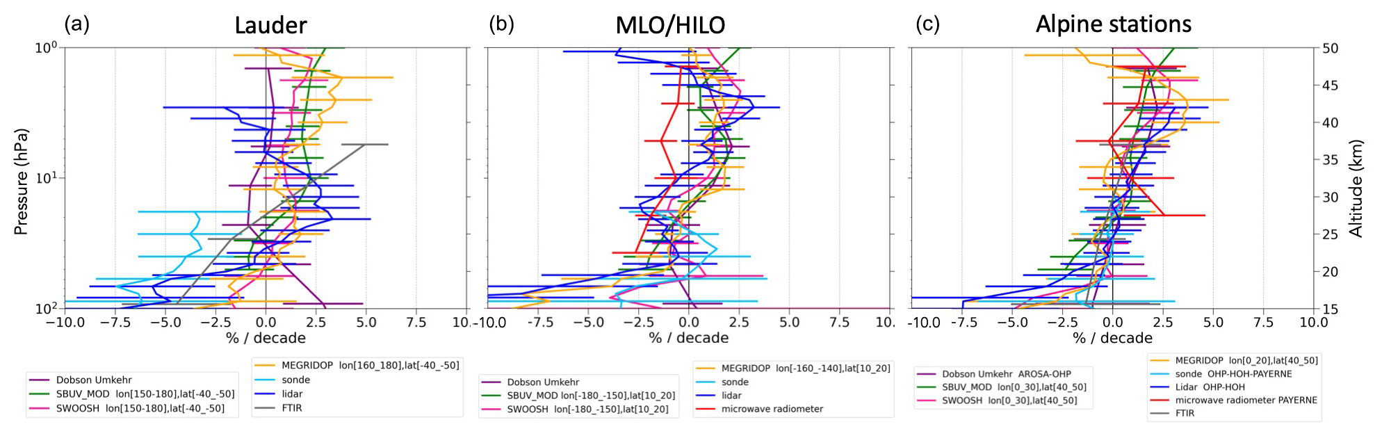
Figure 4Ozone profile trends for the post-2000 periods from selected ground-based NDACC stations. (a) SH Lauder station, (b) tropical Mauna Loa and Hilo (ozonesondes) stations, (c) NH Alpine stations (see text).
4.3 Combined trends
The various trend profiles in broad latitude bands were combined in order to facilitate comparison with LOTUS19 results and with CCMI-1 simulations. We adopted the same methodology as in LOTUS19. The combined trend corresponds to the unweighted mean of the seven trend profiles shown in Fig. 2. At pressures larger than 50 hPa level, the mean combines the results from five data records, since SBUV data in the lowermost stratosphere should not be considered. The average is calculated after converting the trends in altitude coordinate to pressure coordinate using a climatological ERA-Interim pressure – temperature profile over the period. For the combined trend uncertainty, we have to take into account the correlation between the individual trend estimates, which is due to the use of common underlying individual satellite records for some of them, e.g. SAGE II for many merged records or OMPS-LP and the various SBUV time series in the case of the SBUV MOD and SBUV COH records. The correlation also comes from similar atmospheric variability not characterized by the regression model (see LOTUS19 for more details). The variance of the mean is estimated as follows:
where σi is the uncertainty of individual trends xi estimated from the fit, is the unweighted mean of the trends, N is the number of averaged records, Ci,j is the correlation coefficient between the fit residuals of merged data records i and j, and neff is the effective number of independent values, evaluated as follows:
In Eq. (3), the first term on the right-hand side corresponds to the variance of the mean based on the classical propagation of errors for correlated variables ( and the second to the variance of the mean for neff independent estimates (. The second term considers additional uncertainties in the trend average that are not identified in the first term but might lead to different trend estimates, such as drifts in the individual time series. More information on this method is given in chap. 5 of LOTUS19 (Sect. 5.3.1). Results of the combined trends from this study, called LOTUS22 hereafter, are displayed in Fig. 3 (red curves) with comparison to the LOTUS19 combined trends (blue curve); see also Fig. S1 in the Supplement for the comparison of LOTUS19 and LOTUS22 trends in both pre-1997 and post-2000 periods. In addition, Table S1 in the Supplement provides the correlation coefficients obtained for LOTUS22. The neff value for the seven merged ozone records is equal to 1.39, compared to 1.37 in LOTUS19, where six records were considered for the trend combination. Figure 3 shows that, compared to LOTUS19, the combined trend uncertainty is significantly smaller, especially in the upper stratosphere across all three broad latitude bands. This confirms the previous findings that ozone is increasing in the upper stratosphere. The increase is somewhat larger in the NH with a maximum trend of ∼2.2 % per decade reached at ∼2.2 hPa, compared to ∼2.1 % per decade at ∼3.2 hPa in the SH and ∼1.6 % per decade at ∼2.6 hPa in the tropics. Uncertainties in the combined trends are also smaller at pressures larger than 10 hPa, except in the Southern Hemisphere midlatitudes, where already mentioned positive trends retrieved from some of the records impact both the combined trend average and its uncertainty. It should be noted that slightly significant negative trends of ∼1% per decade are retrieved in the tropics in the 30–40 hPa range. In the lowermost stratosphere, i.e. at pressures larger than 50 hPa, the LOTUS22 combined trends are negative and systematically larger in magnitude than the LOTUS19 derived trends. In the tropics, the trend uncertainty in our study increases, so that although the negative trends also increase in magnitude, they are not significant, as in LOTUS19. In the SH and NH lower stratosphere, the difference between both combined trends is very small, although LOTUS22 provides slightly more negative trends, also with smaller uncertainty. In all cases and as noted previously, the uncertainties are large and preclude any definitive conclusion about ozone long-term changes in the lowermost stratosphere.
4.4 Trends over selected NDACC stations
The results of comparisons between ground-based and merged satellite ozone trends for the selected NDACC stations are displayed in Fig. 4. The merged satellite records are MEGRIDOP, SWOOSH and SBUV MOD, for which longitudinally resolved data were provided. We use the satellite data in the grid cell closest to the stations for the trend computation. For the ground-based results in the Alpine stations, trends correspond to the average trend of the following records: (1) ozonesondes – Hohenpeißenberg, Payerne and OHP; (2) lidar – Hohenpeißenberg and OHP; (3) Umkehr – Arosa and OHP; (4) FTIR – Zugspitze and Jungfraujoch; (5) MWR – Payerne. For MWR trends, we used the Payerne record only, as some calibration problems were found in the MWR Bern record. In LOTUS19, trends from ground-based instruments were compared to the combined trends from merged satellite records in broad latitude bands. This is different from the more direct comparison performed in the present study. Figure 4 shows a general good agreement between the ground-based and the gridded satellite trends for the NH Alpine and tropical stations, usually well within the respective uncertainties. Trend results differ more at the Lauder station. Results from the Alpine ground-based measurements reproduce the trend patterns observed with the merged satellite records quite well, e.g. an increase of about 2 % per decade on average in the upper stratosphere, trend values around zero in the middle stratosphere and mostly negative trends below 20 km, with large uncertainties. It is interesting to see that gridded satellite trend results, which rely on more individual data points, differ as much as the ground-based ones in the upper stratosphere.
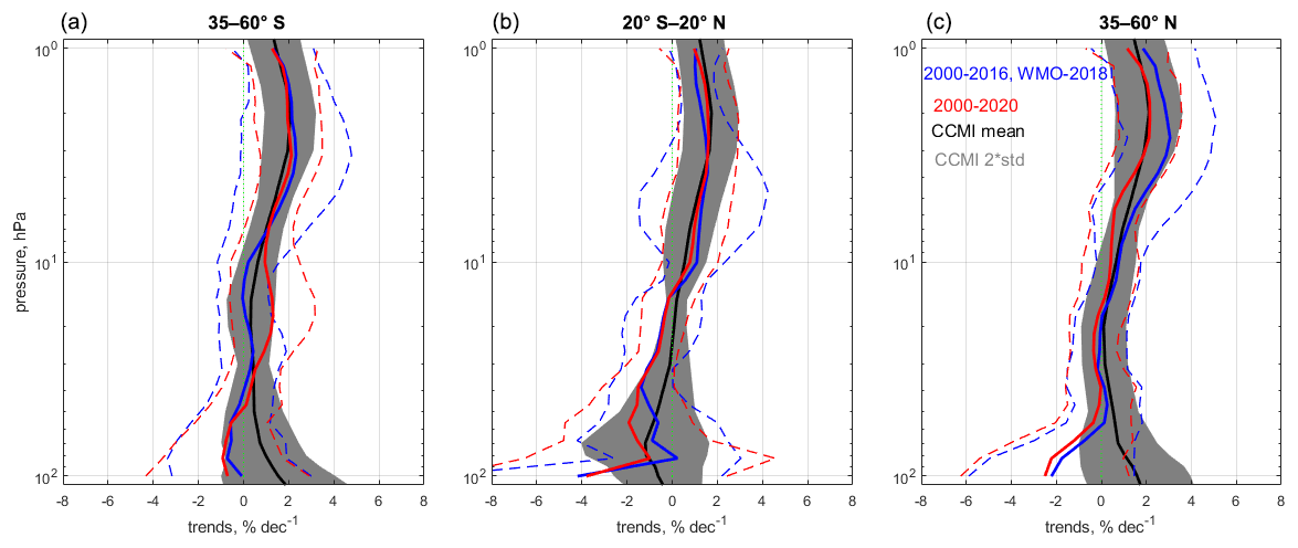
Figure 5Black line: multi-model mean ozone profile trend estimates from the CCMI-1 REF-C2 simulations over three broad latitude bands (a 60–35∘ S, b 20∘ S–20∘ N, c 35–60∘ N). Grey envelope: 2σ uncertainty of the multi-model mean trend estimates. Red (blue) lines and light red (light blue) dashed lines represent LOTUS22 (LOTUS19) average and 2σ uncertainty respectively.
At Mauna Loa and Hilo, similar patterns emerge also with (1) an ozone increase in most records in the upper stratosphere, except the MWR trend, (2) very small negative trends in the middle stratosphere that are most pronounced with the lidar record, and (3) larger negative trends in absolute values in the lower stratosphere below 20 km. For MEGRIDOP and the lidar, negative trends are significant in this altitude region. Compared to Fig. 5.10 of LOTUS19, ozonesondes and Umkehr results now show a better agreement with the other records. Regarding the MWR, it should be noted that there were major upgrades to the MLO MWR instrument from 2015–2017, including the replacement of the filterbank spectrometer with a fast Fourier transform (FFT) spectrometer, which induced a gap in the dataset.
At Lauder, the trend profiles still show larger differences, which were not reduced compared to LOTUS19, despite the homogenization of the ozonesondes and Umkehr records. Trend results from MWR data are not shown as the record was not extended after 2016. Most records show positive trends in the upper stratosphere except for the lidar and Umkehr records. Gridded satellite data trends are in between the ground-based ones in this altitude range. In the lowermost stratosphere, negative trends are obtained from most records except from Umkehr. The largest negative trends in absolute values are retrieved from the ozonesondes and lidar records.
In conclusion, trend comparison between ground-based and longitudinally resolved satellite records provides a similar picture as in the previous section, more specifically (1) positive and significant ozone trends in the upper stratosphere from most of the records, (2) negligible trends in the middle stratosphere, and (3) negative trends below 20 km, which are statistically significant in lidar and ozonesonde records.
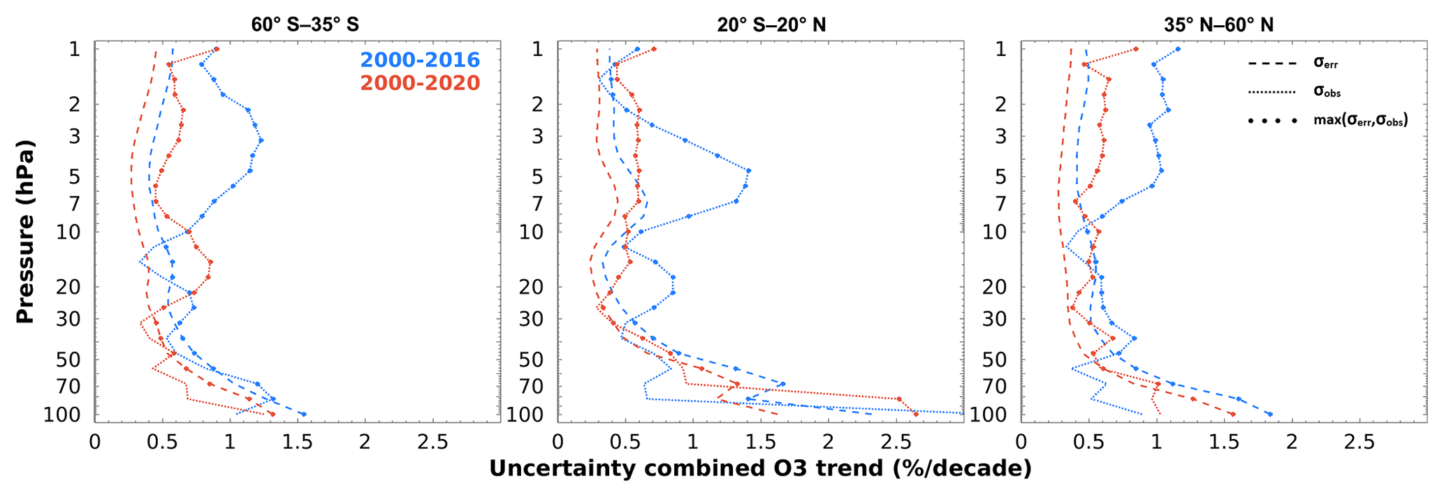
Figure 6Decomposition of error terms for the combine trend estimates: propagation of errors from fit residuals (σerr, dashed lines) and standard error of the trend sample (σobs, dotted lines) for LOTUS22 in red and LOTUS19 in blue for the three broad latitude bands. Combined trend uncertainty is shown by circle symbols that indicate the maximum of σerr and σobs in each case.
4.5 Comparison with trends derived from CCMI-1 simulations
The comparison of CCMI-1 trend results and merged satellite combined trends (LOTUS22) is displayed in Fig. 5, which also includes results from LOTUS19. In the figure, multi-model mean trend estimates from the CCMI-1 REF-C2 simulations are represented by the black line, and the 2σ uncertainty of the multi-model mean trend estimates is given by the grey envelope. Red (blue) solid curves show LOTUS22 (LOTUS19) combined trends respectively with corresponding 2σ uncertainties (Eq. 3) represented by the dashed lines. The individual model trends (from a total of 16 CCMI-1 models, as in LOTUS19) are estimated using the ILT regression method in the same way as for the satellite data and are then combined into a multi-model mean. Model simulations are updated to include 2020, and the necessary proxies are calculated directly from the relevant individual model simulations where appropriate (e.g. QBO, ENSO) or taken from the external forcings provided to the modelling groups. Figure 5 shows very good agreement between the CCMI-1 and LOTUS22 trend estimates in the upper stratosphere, both regarding the average trend values and the uncertainties. In the Northern Hemisphere, the agreement is improved compared to the LOTUS19 results. In the middle stratosphere, some differences are observed, e.g. in the Southern Hemisphere, where the LOTUS22 trends are positive with large uncertainties, in contrast to CCMI-1 and LOTUS19 observed trends, which are very close to zero. In the lowermost stratosphere, observed and simulated trend values diverge at midlatitudes of both hemispheres, with positive non-significant trends from the CCMI-1 simulations and negative but also non-significant trends from LOTUS19 and LOTUS22. Agreement is better in the tropics, where CCMI and both LOTUS studies show small, although non-significant, negative trends. In conclusion, the LOTUS22 trend results confirm the findings of LOTUS19 and provide observed trends that are consistent in magnitude and uncertainty range with simulated ozone trends from the CCMI initiative.
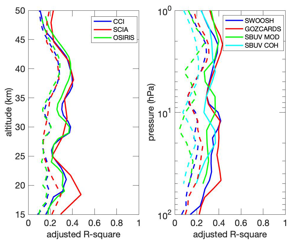
Figure 7Adjusted R2 values of the LOTUS regression model using seasonal (solid lines) and non-seasonal (dashed lines) variation in fitted coefficients in the LOTUS regression model (see text).
In this section, we discuss in more detail the differences in trend estimates between LOTUS19 and LOTUS22. Compared to Fig. 5.6 of the LOTUS19 report, the agreement between the merged datasets is improved, resulting in smaller uncertainties in the combined trend results. This improvement is to a large extent driven by a better agreement of trend results between both SBUV merged records, e.g. SBUV MOD and SBUV COH, due to revised inter-calibration of the individual SBUV records and the addition of OMPS in both merged datasets. Trends from these datasets now agree better with other records' trends, especially in the upper stratosphere. We can have a better understanding of the improvement in trend uncertainties from Fig. 6, which displays the square root of both terms included in the variance of the combined trend (Eq. 3), i.e. the term linked to error propagation (left term on the right side in Eq. (3), σerr, dashed line) and that linked to the standard error of the trend sample (right term of the right term in Eq. (3), σobs, dotted line) for LOTUS22 in red and LOTUS19 in blue. The three panels correspond to the three broad latitude bands. As indicated in Eq. (3), the reported uncertainty value is the maximum of both terms as a function of pressure. We can see from the figure that in both studies the uncertainty is dominated by the σobs term in the upper and middle stratosphere and by the σerr term in the lowermost stratosphere. Reduction in the σobs term from LOTUS19 to LOTUS22 is clearly visible in the figure. It is most pronounced in the tropics around 5 hPa, then in the SH in the 5–1 hPa pressure range, and in the NH to a somewhat lower extent in the same pressure range. The LOTUS22 σobs term is also reduced in the tropical middle stratosphere, but it is increased with respect to LOTUS19 at southern midlatitudes in about the same pressure range. This is due to the already mentioned positive trends retrieved by most of the records at this latitude and pressure range. In the lowermost stratosphere, the dominance of the σerr term is expected due to the large uncertainty retrieved for the trends of the majority of the records in this altitude range.
Another factor that allowed us to reduce the uncertainty of our trend retrieval is the improvement of the LOTUS trend model that now includes seasonal terms for the fitted coefficients (as described in Sect. 3). Thanks to this improvement, the model now better fits the ozone variability of the various records. This is shown in Fig. 7, which displays adjusted R2 values of the regression in broad latitude bands for the records with altitude as a vertical coordinate on the left and those with pressure on the right. Adjusted R2 provides an estimation of the amount of variance in the monthly data explained by the regression model. It is an indicator of the goodness of the fit. Displayed R2 values correspond to the average of R2 profiles for the three latitude bands considered in the study. Solid (dashed) lines show R2 values retrieved from the LOTUS model with seasonal (non-seasonal) variation in the fitted coefficients. Larger R2 values are systematically obtained with seasonal variation of the fitted coefficients.
Using both the improved merged satellite records for this study and the new version of the LOTUS regression model, we can further constrain ozone trends in the various altitude and latitude regions.
This study provides an updated evaluation of stratospheric ozone profile trends in the 60∘ S–60∘ N latitude range from up-to-date merged satellite and ground-based records. Some satellite data series were improved with respect to those used in the previous assessments (WMO, 2018, and LOTUS19), e.g. SBUV MOD and SBUV COH, which resulted in a better agreement between trends from both records and with the other ones used in the study. Additional records that were absent from the LOTUS19 study are included, e.g. the SAGE-SCIAMACHY-OMPS and MEGRIDOP records. Regarding ground-based data, we use ECC homogenized ozonesonde and Umkehr data reprocessed with an optimized homogenization technique that were not available previously. An updated version of the LOTUS regression trend model allows us to improve the fit of ozone variability for the various records. With these improvements, we can draw the following conclusions.
The increase in ozone in the upper stratosphere at pressures lower than 5 hPa is confirmed, with a clearer recovery in the Southern Hemisphere compared to LOTUS19. In this altitude region, combined satellite trends are significant in the three broad latitude bands considered, i.e. the southern and northern midlatitudes and tropics.
In the middle stratosphere, i.e. between 50 and 10 hPa, we see the emergence of new signals that will need to be confirmed in the future: an increase in ozone in the Southern Hemisphere midlatitudes of about 1.2 % per decade, although non-significant, and an ozone decrease in the tropics that is (just) significant at around 35 hPa. In the Northern Hemisphere, ozone trends are close to zero in this altitude range.
In the lower and lowermost stratosphere, negative ozone trends are obtained for all latitude bands, as in LOTUS19. Trends are negligible in the southern midlatitudes. The trends amount to about −2 % per decade in the tropics and are non-significant due to the large uncertainties. Negative ozone trends are also obtained in the Northern Hemisphere, mainly at pressures larger than 70 hPa. They reach −2 % per decade at 100 hPa but are also non-significant.
Comparison of combined trends with those derived from updated CCMI-1 simulations in broad latitude bands shows very good agreement in the upper stratosphere, both in trend magnitude and uncertainty. Larger differences are seen below 10, 40 and 60 hPa in the tropics, SH, and NH midlatitudes respectively with the CCMI-1 trends being generally more positive than the satellite ones. Differences are most pronounced in the NH midlatitudes, where average satellite trends are negative, while those of CCMI-1 are positive. Due to the large uncertainty in both cases, these differences are non-significant.
Compared to LOTUS19, we find a better agreement between trends from ground-based measurements and from satellite records, especially in the tropics and in the Alpine stations of the Northern Hemisphere, for most of the records. This can be due to both the use of longitudinally resolved satellite data and to improved ground-based and satellite records. Trends values are more scattered at the Lauder station. The differences between trends from longitudinally resolved satellite records and some ground-based time series at the selected NDACC stations warrant more detailed analyses in the future, focusing on the possible biases between the records.
The ozone recovery signal that is mainly observed in the upper stratosphere has an influence on total ozone trends. A recent study indicates a total ozone recovery of 0.5±0.2 % per decade (∼1.5 DU per decade) since 1996 (Weber et al., 2022). However, total column ozone evolution is influenced even more by trends in the lower stratosphere and also by tropospheric ozone trends. The latter are estimated to be of the order of ∼1.5 DU per decade (e.g. Gaudel et al., 2018; Ziemke et al., 2019) with larger changes found in the tropical regions. The precise impact of stratospheric and tropospheric partial ozone column trends on total column ozone trends thus needs further evaluation.
The consistency of ozone profile trends found in this study demonstrates that the global ozone observing system is still robust, thanks to the continuing and improved satellite and ground-based records. This allows us to quite accurately evaluate long-term ozone changes in the stratosphere. The cause of some larger discrepancies between combined satellite and CCMI trends in the lower stratosphere will have to be further investigated, as the new set of CCMI-2022 simulations becomes available (Plummer et al., 2021). More generally, the study of ozone trends in this region may require a special focus with geophysically based coordinate systems, using, e.g., tropopause level or equivalent latitude (Millan et al., 2021) in order to better constrain ozone variability and provide a more accurate trend evaluation.
The various data and model records used in this article are available in the following depository: https://doi.org/10.5281/zenodo.6958560 (Godin-Beekmann et al., 2022).
Information about the most recent versions of each dataset can be found at their individual source locations:
Merged satellite datasets:
-
SBUV MOD: https://acd-ext.gsfc.nasa.gov/Data_services/merged/index.html (NASA GSFC, USA, last access: June 2022).
-
SBUV COH: https://ftp.cpc.ncep.noaa.gov/SBUV_CDR/ (NOAA, USA, last access: 22 June 2022).
-
GOZCARDS: https://www.earthdata.nasa.gov/esds/competitive-programs/measures/gozcards (NASA, USA, last access: 22 June 2022).
-
SWOOSH: https://csl.noaa.gov/groups/csl8/swoosh/ (NOAA, USA, last access: 22 June 2022).
-
SAGE-CCI-OMPS and MEGRIDOP datasets are available through https://climate.esa.int/en/projects/ozone/data/ and ftp://cci_web@ftp-ae.oma.be/esacci (ESA Climate Office, last access: 10 August 2022). They are provided by FMI, Finland.
-
SAGE-SCIAMACHY-OMPS: data record is available upon registration via the following link: https://www.iup.uni-bremen.de/DataRequest/ (U. Bremen, Germany, last access: 22 June 2022).
-
SAGE-OSIRIS-OMPS: downloading instructions can be found at https://research-groups.usask.ca/osiris/data-products.php#OSIRISLevel3andMergedDataProducts (U. Saskatchewan, Canada, last access: 22 June 2022).
Ground-based records:
-
Umkehr: https://gml.noaa.gov/aftp/data/ozwv/Dobson/AC4/Umkehr/Monthly/ (NOAA, USA, last access: 22 June 2022).
-
Ozonesondes: https://hegiftom.meteo.be/datasets/ozonesondes (HEGIFTOM, last access: 22 June 2022). Measurements at the various stations are provided by the following institutions:
-
Hohenpeissenberg: DWD, Germany
-
Payerne: MeteoSwiss, Switzerland
-
OHP: CNRS, France
-
Hilo: NOAA, USA
-
Lauder: NIWA, New Zealand.
-
-
Lidar: http://www.ndacc.org/ (last access: 22 June 2022). Measurements at the various stations are provided by the following institutions:
-
Hohenpeissenberg: DWD, Germany
-
OHP: CNRS, France
-
MLO: JPL, NASA, USA
-
Lauder: NIWA, New Zealand.
-
-
FTIR spectrometers: http://www.ndacc.org/ (last access: 22 June 2022). Measurements at the various stations are provided by the following institutions:
-
Zugspitze: KIT, Germany
-
Jungfraujoch: ULiège, GIRPAS team, Belgium
-
Lauder: NIWA, New Zealand.
-
-
Microwave spectrometers: http://www.ndacc.org/ (last access: 22 June 2022). Measurements at the various stations are provided by the following institutions:
-
Payerne: MeteoSwiss, Switzerland
-
Mauna Loa: NRL, USA
-
Lauder: NRL, USA.
Chemistry climate model (CCM) simulations:
https://blogs.reading.ac.uk/ccmi (last access: 10 August 2022). -
The supplement related to this article is available online at: https://doi.org/10.5194/acp-22-11657-2022-supplement.
NA computed the satellite and ground-based trends, VS computed the combined trends and provided Figs. 4 and S1, DH provided Figs. 3 and 6, KT provided the trends from CCMI-1 simulations, and DAD, DZ and RD provided and maintain the LOTUS regression model. Other co-authors contributed with satellite or ground-based data. The results of the study were discussed by all the co-authors. The paper was written by SGB with supporting comments by all co-authors.
At least one of the (co-)authors is a guest member of the editorial board of Atmospheric Chemistry and Physics for the special issue “Atmospheric ozone and related species in the early 2020s: latest results and trends (ACP/AMT inter-journal SI), 2021”. The peer-review process was guided by an independent editor, and the authors also have no other competing interests to declare.
Publisher's note: Copernicus Publications remains neutral with regard to jurisdictional claims in published maps and institutional affiliations.
This article is part of the special issue “Atmospheric ozone and related species in the early 2020s: latest results and trends (ACP/AMT inter-journal SI)”.
The ground-based data used in this publication were obtained as part of the Network for the Detection of Atmospheric Composition Change (NDACC) and are available through the NDACC website http://www.ndacc.org/ (last access: 22 June 2022). Optimized Umkehr data are available at https://gml.noaa.gov/aftp/data/ozwv/Dobson/AC4/Umkehr/Optimized/ (last access: 22 June 2022). Homogenized ozonesonde data were obtained though the HEGIFTOM Focus Working Group: https://hegiftom.meteo.be/ (last access: 22 June 2022). Niramson Azouz's work was supported by a postdoctoral fellowship from Institut National des Sciences de l'Univers du Centre National de la Recherche Scientifique (INSU-CNRS). Work at the Jet Propulsion Laboratory, California Institute of Technology, was performed under contract with the National Aeronautics and Space Administration (80NM0018D004); we gratefully acknowledge the efforts of Ray Wang, John Anderson and Ryan Fuller towards the initial GOZCARDS ozone data record and its subsequent updates. Irina Petropavlovskikh and Jeannette Wild were supported by NOAA Climate Program Office's Atmospheric Chemistry, Carbon Cycle, and Climate programme, grant number NA19OAR4310169 (CU)/NA19OAR4310171 (UMD). The SBUV Merged Ozone Data Set was constructed under the NASA MeaSUREs Project and is maintained under NASA WBS 479717 (Long Term Measurement of Ozone). Carlo Arosio acknowledges the support of the University and State of Bremen, and the funding from DAAD and the Living Planet Fellowship SOLVE. The SAGE-CCI-OMPS and MEGRIDOP datasets are created in the framework of ESA Ozone-CCI+ project. The work of Viktoria Sofieva was supported by the European Space Agency (Ozone_cci+ project, contract 4000126562/19/I-NB), the EU Copernicus Climate Change Service for Atmospheric Composition ECVs (contract C3S_312b_Lot2_DLR_2018SC1) and the Academy of Finland (the Centre of Excellence of Inverse Modelling and Imaging (decision 336798). The multi-decadal monitoring programme of the University of Liège at the Jungfraujoch station has been primarily supported by the F.R.S.-FNRS and BELSPO (both in Brussels, Belgium) and by the GAW-CH programme of MeteoSwiss. The International Foundation High Altitude Research Stations Jungfraujoch and Gornergrat (HFSJG, Bern) supported the facilities needed to perform the FTIR observations. The OSIRIS data are made available through the continued support of the Canadian Space Agency. The FTIR site Zugspitze has been supported by the Helmholtz Society via the research programme ATMO.
This research has been supported by CNRS-INSU through the fellowship of Niramson Azouz.
This paper was edited by Martin Dameris and reviewed by two anonymous referees.
Arosio, C., Rozanov, A., Malinina, E., Weber, M., and Burrows, J. P.: Merging of ozone profiles from SCIAMACHY, OMPS and SAGE II observations to study stratospheric ozone changes, Atmos. Meas. Tech., 12, 2423–2444, https://doi.org/10.5194/amt-12-2423-2019, 2019.
Ball, W. T., Alsing, J., Mortlock, D. J., Staehelin, J., Haigh, J. D., Peter, T., Tummon, F., Stübi, R., Stenke, A., Anderson, J., Bourassa, A., Davis, S. M., Degenstein, D., Frith, S., Froidevaux, L., Roth, C., Sofieva, V., Wang, R., Wild, J., Yu, P., Ziemke, J. R., and Rozanov, E. V.: Evidence for a continuous decline in lower stratospheric ozone offsetting ozone layer recovery, Atmos. Chem. Phys., 18, 1379–1394, https://doi.org/10.5194/acp-18-1379-2018, 2018.
Ball, W. T., Chiodo, G., Abalos, M., Alsing, J., and Stenke, A.: Inconsistencies between chemistry–climate models and observed lower stratospheric ozone trends since 1998, Atmos. Chem. Phys., 20, 9737–9752, https://doi.org/10.5194/acp-20-9737-2020, 2020.
Bernet, L., von Clarmann, T., Godin-Beekmann, S., Ancellet, G., Maillard Barras, E., Stübi, R., Steinbrecht, W., Kämpfer, N., and Hocke, K.: Ground-based ozone profiles over central Europe: incorporating anomalous observations into the analysis of stratospheric ozone trends, Atmos. Chem. Phys., 19, 4289–4309, https://doi.org/10.5194/acp-19-4289-2019, 2019.
Bourassa, A. E., Roth, C. Z., Zawada, D. J., Rieger, L. A., McLinden, C. A., and Degenstein, D. A.: Drift-corrected Odin-OSIRIS ozone product: algorithm and updated stratospheric ozone trends, Atmos. Meas. Tech., 11, 489–498, https://doi.org/10.5194/amt-11-489-2018, 2018.
Chipperfield, M. P., Dhomse, S., Hossaini, R., Feng, W., Santee, M. L., Weber, M., Burrows, J. P., Wild, J. D., Loyola, D., and Coldewey-Egbers, M.: On the Cause of Recent Variations in Lower Stratospheric Ozone, Geophys. Res. Lett., 45, 5718–5726, https://doi.org/10.1029/2018GL078071, 2018.
Cochrane, D. and Orcutt, G. H.: Application of Least Squares Regression to Relationships Containing Auto-Correlated Error Term, J. Am. Stat. Assoc., 44, 32–61, https://doi.org/10.1080/01621459.1949.10483290, 1949.
Davis, S. M., Rosenlof, K. H., Hassler, B., Hurst, D. F., Read, W. G., Vömel, H., Selkirk, H., Fujiwara, M., and Damadeo, R.: The Stratospheric Water and Ozone Satellite Homogenized (SWOOSH) database: a long-term database for climate studies, Earth Syst. Sci. Data, 8, 461–490, https://doi.org/10.5194/essd-8-461-2016, 2016.
de Laat, A. T. J., van der A, R. J., and van Weele, M.: Tracing the second stage of ozone recovery in the Antarctic ozone-hole with a “big data” approach to multivariate regressions, Atmos. Chem. Phys., 15, 79–97, https://doi.org/10.5194/acp-15-79-2015, 2015.
Eyring, V., Arblaster, J. M., Cionni, I., Sedlácek, J., Perlwitz, J., Young, P. J., Bekki, S., Bergmann, S., Cameron-Smith, P., Collins, W. J., Faluvegi, G., Gottschaldt, K.-D., Horowitz, L. W., Kinnison, D. E., Lamarque, J.-F., Marsh, D. R., Saint-Martin, D., Shindell, D. T., Sudo, K., Szopa, S., and Watanabe, S.: Long-term ozone changes and associated climate impacts in CMIP5 simulations, J. Geophys. Res. Atmos., 118, 5029–5060, https://doi.org/10.1002/jgrd.50316, 2013.
Frith, S. M., Stolarski, R. S., Kramarova, N. A., and McPeters, R. D.: Estimating uncertainties in the SBUV Version 8.6 merged profile ozone data set, Atmos. Chem. Phys., 17, 14695–14707, https://doi.org/10.5194/acp-17-14695-2017, 2017.
Frith, S. M., Bhartia, P. K., Oman, L. D., Kramarova, N. A., McPeters, R. D., and Labow, G. J.: Model-based climatology of diurnal variability in stratospheric ozone as a data analysis tool, Atmos. Meas. Tech., 13, 2733–2749, https://doi.org/10.5194/amt-13-2733-2020, 2020.
Garcia, R. R. and Randel, W. J.: Acceleration of the Brewer–Dobson circulation due to increases in greenhouse gases, J. Atmos. Sci., 65, 2731–2739, https://doi.org/10.1175/2008JAS2712.1, 2008.
Godin-Beekmann, S., Porteneuve, J., and Garnier, A.: Systematic DIAL ozone measurements at Observatoire de Haute-Provence, J. Env. Monitor., 5, 57–67, 2003.
Godin-Beekmann, S., Sofieva, V. F., Petropavlovskikh, I., Effertz, P., Ancellet, G., Degenstein, D. A., Froidevaux, L., Frith, S., Wild, J., Davis, S., Steinbrecht, W., Leblanc, T., Querel, R., Tourpali, K., Barras, E. M., Stübi, R., Vigouroux, C., Arosio, C., Nedoluha, G. et al.: data sets from “Updated trends of the stratospheric ozone vertical distribution in the 60∘ S–60∘ N latitude range based on the LOTUS regression model”, Zenodo [data set], https://doi.org/10.5281/zenodo.6958560, 2022.
Hase, F., Blumenstock, T., and Paton-Walsh, C., Analysis of the instrumental line shape of high-resolution Fou-rier transform IR spectrometers with gas cell measurements and new retrieval software, Appl. Opt., 38, 3417–3422, https://doi.org/10.1364/AO.38.003417, 1999.
Harris, N. R. P., Hassler, B., Tummon, F., Bodeker, G. E., Hubert, D., Petropavlovskikh, I., Steinbrecht, W., Anderson, J., Bhartia, P. K., Boone, C. D., Bourassa, A., Davis, S. M., Degenstein, D., Delcloo, A., Frith, S. M., Froidevaux, L., Godin-Beekmann, S., Jones, N., Kurylo, M. J., Kyrölä, E., Laine, M., Leblanc, S. T., Lambert, J.-C., Liley, B., Mahieu, E., Maycock, A., de Mazière, M., Parrish, A., Querel, R., Rosenlof, K. H., Roth, C., Sioris, C., Staehelin, J., Stolarski, R. S., Stübi, R., Tamminen, J., Vigouroux, C., Walker, K. A., Wang, H. J., Wild, J., and Zawodny, J. M.: Past changes in the vertical distribution of ozone – Part 3: Analysis and interpretation of trends, Atmos. Chem. Phys., 15, 9965–9982, https://doi.org/10.5194/acp-15-9965-2015, 2015.
Hegglin, M. I., Lamarque, J.-F., Duncan, B., Eyring, V., Gettelman, A., Hess, P., Myhre, G., Nagashima, T., Plummer, D., Ryerson, T., Shepherd, T., and Waugh, D.: Report on the IGAC/SPARC Chemistry-Climate Model Initiative (CCMI) 2015 science workshop, SPARC Newsl., 46, 37–42, 2016.
Leblanc, T., Sica, R. J., van Gijsel, J. A. E., Godin-Beekmann, S., Haefele, A., Trickl, T., Payen, G., and Liberti, G.: Proposed standardized definitions for vertical resolution and uncertainty in the NDACC lidar ozone and temperature algorithms – Part 2: Ozone DIAL uncertainty budget, Atmos. Meas. Tech., 9, 4051–4078, https://doi.org/10.5194/amt-9-4051-2016, 2016.
Maillard Barras, E., Haefele, A., Nguyen, L., Tummon, F., Ball, W. T., Rozanov, E. V., Rüfenacht, R., Hocke, K., Bernet, L., Kämpfer, N., Nedoluha, G., and Boyd, I.: Study of the dependence of long-term stratospheric ozone trends on local solar time, Atmos. Chem. Phys., 20, 8453–8471, https://doi.org/10.5194/acp-20-8453-2020, 2020.
Millán, L. F., Manney, G. L., and Lawrence, Z. D.: Reanalysis intercomparison of potential vorticity and potential-vorticity-based diagnostics, Atmos. Chem. Phys., 21, 5355–5376, https://doi.org/10.5194/acp-21-5355-2021, 2021.
Morgenstern, O., Hegglin, M. I., Rozanov, E., O'Connor, F. M., Abraham, N. L., Akiyoshi, H., Archibald, A. T., Bekki, S., Butchart, N., Chipperfield, M. P., Deushi, M., Dhomse, S. S., Garcia, R. R., Hardiman, S. C., Horowitz, L. W., Jöckel, P., Josse, B., Kinnison, D., Lin, M., Mancini, E., Manyin, M. E., Marchand, M., Marécal, V., Michou, M., Oman, L. D., Pitari, G., Plummer, D. A., Revell, L. E., Saint-Martin, D., Schofield, R., Stenke, A., Stone, K., Sudo, K., Tanaka, T. Y., Tilmes, S., Yamashita, Y., Yoshida, K., and Zeng, G.: Review of the global models used within phase 1 of the Chemistry–Climate Model Initiative (CCMI), Geosci. Model Dev., 10, 639–671, https://doi.org/10.5194/gmd-10-639-2017, 2017.
Newman, P. A., Daniel, J. S., Waugh, D. W., and Nash, E. R.: A new formulation of equivalent effective stratospheric chlorine (EESC), Atmos. Chem. Phys., 7, 4537–4552, https://doi.org/10.5194/acp-7-4537-2007, 2007.
Orbe, C., Wargan, K., Pawson, S., and Oman, L. D.: Mechanisms linked to recent ozone decreases in the Northern Hemisphere lower stratosphere, J. Geophys. Res.-Atmos., 125, e2019JD031631, https://doi.org/10.1029/2019JD031631, 2020.
Pazmiño, A., Godin-Beekmann, S., Hauchecorne, A., Claud, C., Khaykin, S., Goutail, F., Wolfram, E., Salvador, J., and Quel, E.: Multiple symptoms of total ozone recovery inside the Antarctic vortex during austral spring, Atmos. Chem. Phys., 18, 7557–7572, https://doi.org/10.5194/acp-18-7557-2018, 2018.
Petropavlovskikh, I., Godin-Beekmann, S., Hubert, D., Damadeo, R., Hassler, B., and Sofieva, V.: SPARC/IO3C/GAW report on Long-term Ozone Trends and Uncertainties in the Stratosphere, SPARC/IO3C/GAW, SPARC Report No. 9, WCRP-17/2018, GAW Report No. 241, https://doi.org/10.17874/f899e57a20b, 2019.
Petropavlovskikh, I., Miyagawa, K., McClure-Beegle, A., Johnson, B., Wild, J., Strahan, S., Wargan, K., Querel, R., Flynn, L., Beach, E., Ancellet, G., and Godin-Beekmann, S.: Optimized Umkehr profile algorithm for ozone trend analyses, Atmos. Meas. Tech., 15, 1849–1870, https://doi.org/10.5194/amt-15-1849-2022, 2022.
Plummer, D., Nagashima, T., Tilmes, S., Archibald, A., et al.: CCMI-2022: A new set of Chemistry-Climate Model Initiative (CCMI) Community Simulations to Update the Assessment of Models and Support Upcoming Ozone Assessment Activities, in SPARC newsletter, July 2021, https://www.sparc-climate.org/wp-content/uploads/sites/5/2021/07/SPARCnewsletter_Jul2021_web.pdf (last access: 22 June 2022), 2021.
Rodgers, C. D.: Inverse Methods for Atmospheric Sounding: Theory and Practice, World Scientific Publishing Co. Pte. Ltd, Singapore https://doi.org/10.1142/3171, 2000.
Smit, H. G. J. and the Panel for the Assessment of Standard Operating Procedures for Ozonesondes (ASOPOS 2.0): Ozonesonde Measurement Principles and Best Operational Practices, World Meteorological Organization, GAW Report, 268, https://library.wmo.int/doc_num.php?explnum_id=10884 (last access: 22 June 2022), 2021.
Sofieva, V. F., Kyrölä, E., Laine, M., Tamminen, J., Degenstein, D., Bourassa, A., Roth, C., Zawada, D., Weber, M., Rozanov, A., Rahpoe, N., Stiller, G., Laeng, A., von Clarmann, T., Walker, K. A., Sheese, P., Hubert, D., van Roozendael, M., Zehner, C., Damadeo, R., Zawodny, J., Kramarova, N., and Bhartia, P. K.: Merged SAGE II, Ozone_cci and OMPS ozone profile dataset and evaluation of ozone trends in the stratosphere, Atmos. Chem. Phys., 17, 12533–12552, https://doi.org/10.5194/acp-17-12533-2017, 2017.
Sofieva, V. F., Szeląg, M., Tamminen, J., Kyrölä, E., Degenstein, D., Roth, C., Zawada, D., Rozanov, A., Arosio, C., Burrows, J. P., Weber, M., Laeng, A., Stiller, G. P., von Clarmann, T., Froidevaux, L., Livesey, N., van Roozendael, M., and Retscher, C.: Measurement report: regional trends of stratospheric ozone evaluated using the MErged GRIdded Dataset of Ozone Profiles (MEGRIDOP), Atmos. Chem. Phys., 21, 6707–6720, https://doi.org/10.5194/acp-21-6707-2021, 2021.
Solomon, S., Ivy, D. J., Kinnison, D., Mills, M. J., Neely, R. R., and Schmidt, A.: Emergence of healing in the Antarctic ozone layer, Science, 353, 269–274, https://doi.org/10.1126/science.aae0061, 2016.
Steinbrecht, W., Froidevaux, L., Fuller, R., Wang, R., Anderson, J., Roth, C., Bourassa, A., Degenstein, D., Damadeo, R., Zawodny, J., Frith, S., McPeters, R., Bhartia, P., Wild, J., Long, C., Davis, S., Rosenlof, K., Sofieva, V., Walker, K., Rahpoe, N., Rozanov, A., Weber, M., Laeng, A., von Clarmann, T., Stiller, G., Kramarova, N., Godin-Beekmann, S., Leblanc, T., Querel, R., Swart, D., Boyd, I., Hocke, K., Kämpfer, N., Maillard Barras, E., Moreira, L., Nedoluha, G., Vigouroux, C., Blumenstock, T., Schneider, M., García, O., Jones, N., Mahieu, E., Smale, D., Kotkamp, M., Robinson, J., Petropavlovskikh, I., Harris, N., Hassler, B., Hubert, D., and Tummon, F.: An update on ozone profile trends for the period 2000 to 2016, Atmos. Chem. Phys., 17, 10675–10690, https://doi.org/10.5194/acp-17-10675-2017, 2017.
Szeląg, M. E., Sofieva, V. F., Degenstein, D., Roth, C., Davis, S., and Froidevaux, L.: Seasonal stratospheric ozone trends over 2000–2018 derived from several merged data sets, Atmos. Chem. Phys., 20, 7035–7047, https://doi.org/10.5194/acp-20-7035-2020, 2020.
Vigouroux, C., Blumenstock, T., Coffey, M., Errera, Q., García, O., Jones, N. B., Hannigan, J. W., Hase, F., Liley, B., Mahieu, E., Mellqvist, J., Notholt, J., Palm, M., Persson, G., Schneider, M., Servais, C., Smale, D., Thölix, L., and De Mazière, M.: Trends of ozone total columns and vertical distribution from FTIR observations at eight NDACC stations around the globe, Atmos. Chem. Phys., 15, 2915–2933, https://doi.org/10.5194/acp-15-2915-2015, 2015.
Wargan, K., Orbe, C., Pawson, S., Ziemke, J. R., Oman, L. D., Olsen, M. A., Coy, L., and Emma Knowland, K.: Recent Decline in Extratropical Lower Stratospheric Ozone Attributed to Circulation Changes, Geophys. Res. Lett., 45, 5166–5176, https://doi.org/10.1029/2018GL077406, 2018.
Wild, J. D., Petropavlovskikh, I. V., McClure, A., Miyagawa, K., Johnson, B. J., Long, C. S., Strahan, S. E., and Wargan, K.: Ozone recovery as detected in NOAA Ground-Based and Satellite Ozone Measurements, poster presented at the American Geophysical Union Fall Meeting, San Francisco, CA, 7–11 December 2019.
WMO (World Meteorological Organization): Scientific Assessment of Ozone Depletion: 2010, Global Ozone Research and Monitoring Project – Report No. 52, 516 pp., Geneva, Switzerland, 2011.
WMO: Scientific Assessment of Ozone Depletion: 2018, Global Ozone Research and Monitoring Project Report, World Meteorological Organization, p. 588, Geneva, Switzerland, 2018.
Zawada, D. J., Rieger, L. A., Bourassa, A. E., and Degenstein, D. A.: Tomographic retrievals of ozone with the OMPS Limb Profiler: algorithm description and preliminary results, Atmos. Meas. Tech., 11, 2375–2393, https://doi.org/10.5194/amt-11-2375-2018, 2018.