the Creative Commons Attribution 4.0 License.
the Creative Commons Attribution 4.0 License.
 | 07 Sep 2022
Comparison of middle- and low-latitude sodium layer from a ground-based lidar network, the Odin satellite, and WACCM–Na model
Christopher J. Scott
Mingjiao Jia
Wuhu Feng
John M. C. Plane
Daniel R. Marsh
Jonas Hedin
Jörg Gumbel
Xiankang Dou
The ground-based measurements obtained from a lidar network and the 6-year OSIRIS (optical spectrograph and infrared imager system) limb-scanning radiance measurements made by the Odin satellite are used to study the climatology of the middle- and low-latitude sodium (Na) layer. Up to January 2021, four Na resonance fluorescence lidars at Beijing (40.5∘ N, 116.0∘ E), Hefei (31.8∘ N, 117.3∘ E), Wuhan (30.5∘ N, 114.4∘ E), and Haikou (19.5∘ N, 109.1∘ E) collected vertical profiles of Na density for a total of 2136 nights (19 587 h). These large datasets provide multi-year routine measurements of the Na layer with exceptionally high temporal and vertical resolution. The lidar measurements are particularly useful for filling in OSIRIS data gaps since the OSIRIS measurements were not made during the dark winter months because they utilize the solar-pumped resonance fluorescence from Na atoms. The observations of Na layers from the ground-based lidars and the satellite are comprehensively compared with a global model of meteoric Na in the atmosphere (WACCM–Na). The lidars present a unique test of OSIRIS and WACCM (Whole Atmosphere Community Climate Model), because they cover the latitude range along 120∘ E longitude in an unusual geographic location with significant gravity wave generation. In general, good agreement is found between lidar observations, satellite measurements, and WACCM simulations. On the other hand, the Na number density from OSIRIS is larger than that from the Na lidars at the four stations within one standard deviation of the OSIRIS monthly average, particularly in autumn and early winter arising from significant uncertainties in Na density retrieved from much less satellite radiance measurements. WACCM underestimates the seasonal variability of the Na layer observed at the lower latitude lidar stations (Wuhan and Haikou). This discrepancy suggests the seasonal variability of vertical constituent transport modelled in WACCM is underestimated because much of the gravity wave spectrum is not captured in the model.
- Article
(20204 KB) - Full-text XML
- BibTeX
- EndNote


The layers of neutral metal atoms exist in the Earth's mesosphere and lower thermosphere (MLT) at altitudes between 75–110 km (Plane, 2003; Plane et al., 2015, 2018). The MLT region is of particular importance because it marks the transition between the lower neutral and upper ionized atmospheres. Metal layers in the MLT can provide a unique way to study the chemical and dynamical processes in this region. The metals ablating from meteoroids entering the atmosphere include Na, Fe, Mg, Al, Ni, Ca, and K (Plane et al., 2015). The first quantitative measurements of metal atoms were made with ground-based photometers in the 1950s by the observations of resonance scattering of sunlight (Hunten, 1967). Na has a suitably large resonant scattering cross-section and a high column abundance as one of the primary meteoric species in the MLT. As a result, the Na atom layer was the first to be discovered and is one of the most researched metal layers (Bowman et al., 1969; Sandford and Gibson, 1970).
Over the last two decades, the space-borne limb-scanning spectrometers have provided a near-global measurement of Na layers. The first global geographical distribution of Na layers was produced by the global ozone monitoring by occultation of stars (GOMOS) spectrometers onboard the Envisat satellite (Fussen et al., 2004), followed by a more detailed study based on 7 years of GOMOS observations (Fussen et al., 2010). The optical spectrograph and infrared imager system (OSIRIS) spectrometer onboard the Odin satellite measures the Na concentration profiles from the limb-scanning observations of Na D-lines at 589 nm in the dayglow (Gumbel et al., 2007; Fan et al., 2007a, b; Plane, 2022; Hedin and Gumbel, 2011; Langowski et al., 2017). The Na profiles retrieved from Odin/OSIRIS typically have an altitude resolution of 2 km and an accuracy of 20 % in the metal density at the layer peak (Gumbel et al., 2007). Koch et al. (2022) presented the comparison of Na measurements between OSIRIS/Odin, GOMOS/Envisat, and SCIAMACHY (SCanning Imaging Absorption spectroMeter for Atmospheric CHartographY)/Envisat. The Na concentration profiles from three space-borne instruments agree well.
Since the first Na lidar measurements in England in the 1960s (Bowman et al., 1969), the light detection and ranging (lidar) technique has permitted long-term routine monitoring of the Na layer (She et al., 2000; Vishnu Prasanth et al., 2009; Krueger et al., 2015; She et al., 2021). Many studies of the diurnal and seasonal variations in the Na layer (Gardner et al., 2005; Yuan et al., 2012; Plane et al., 2015; Li et al., 2018), and the dynamical and chemical coupling between ionized and neutral metals (Yuan et al., 2014b; Yu et al., 2019a; Xia et al., 2020) have resulted from the substantial growth in ground-based Na lidar stations making Na measurements in recent decades. Sporadic sodium layers (SSLs), characterized by a sudden increase of Na atoms in a narrow altitude range, have been of particular interest. The SSL was first reported by Clemesha et al. (1978) from Na lidar observations, and such an extremely narrow and sharp increase in Na atom density could not be produced by neutral density perturbations. The high-resolution observations of the Na density show large-scale instabilities and Kelvin–Helmholtz billows with the downward propagating SSLs (Pfrommer et al., 2009). The sporadic E (Es) layers, thin layers of concentrated metallic plasma in the lower E region of the ionosphere, are proposed to be a source of sodium in the mesosphere (Plane, 2012). Studies show that the SSLs are closely related to the changes in Na+ metallic ions within Es layers (Yuan et al., 2014b; Qiu et al., 2018; Cai et al., 2019a, b; Xia et al., 2021). From a laboratory kinetic study, Cox and Plane (1998) demonstrated that the sporadic metal layer is produced when the Es layer descends below 100 km under the influence of tides. Further observations have confirmed the strong coupling between the SSLs and Es layers (Cox and Plane, 1998; Dou et al., 2010; Williams et al., 2007; Dou et al., 2013; Yuan et al., 2013; Qiu et al., 2016; S. Qiu et al., 2021). The simulation results show that the variation in the climatology of Na density in summer at mid-latitudes is modulated by the convergence of metallic ions with a descending Es layer through the prevailing descent of tidal wind shear (Cai et al., 2017). Na lidars can provide continuous local measurements of the Na layer with exceptionally high temporal and vertical resolution (usually 3 min and 0.1 km), and only provide point measurements, which is a severe constraint. As a result, it is not possible to obtain a global distribution of the Na layer using ground-based lidars.
Many modelling studies have focused on simulating the seasonal and short-term variability of metallic ions and atoms (Feng et al., 2013; Marsh et al., 2013; Cai et al., 2019a, b). Global climate models generally focus on large-scale advection and eddy diffusion transport, but they do not resolve the omnipresent small-scale waves and turbulence fluctuations (Marsh et al., 2007). However, dynamical and chemical constituent transport in the MLT is significantly impacted by dissipating gravity waves (Gardner and Liu, 2016). It has been shown that the meteoric influx employed in the Whole Atmosphere Community Climate Model (WACCM) is much smaller, by a factor of approximately 5, than the actual vertical flux from Na lidar measurements (Gardner and Liu, 2014), which suggests that the vertical transport of atmospheric constituents (e.g. Na and Fe) as modelled in WACCM is too slow (Gardner and Liu, 2016). Data–model comparison between lidars and WACCM is important to understand wave-driven dynamical and chemical processes of atmospheric metals in the MLT.
A ground-based network of four Na lidars has been routinely operated in the Chinese Meridian Project (CMP) over the last decade (Wang, 2010). The lidars range from low- to mid-latitudes roughly along 120∘ E longitude in China. These lidars are in an unusual geographic location with significant gravity wave generation (Hocke et al., 2016; Zeng et al., 2017). By the year 2021, a total of 2136 nights (19 587 h) of vertical profiles of Na density were obtained. The lidar observations provide an important test of Odin satellite measurements and WACCM simulations, allowing us to investigate the impact of waves and turbulence fluctuations on the WACCM predictions of Na density. It should be noted that the original ground-truthing of Odin measurements involved Na lidar measurements at Fort Collins, Colorado which is at a latitude of 41∘ N (Gumbel et al., 2007).
The present paper is therefore a study of the latitudinal and seasonal variations of the Na layer at mid- and low-latitudes, using a combination of the Odin satellite measurements, the multi-year ground-based measurements obtained from the lidar network, and the WACCM–Na model. The Na lidar data are compared to the sun-synchronous satellite measurements at descending and ascending nodes and simultaneous WACCM simulations. Section 2 describes the instruments and datasets. In Sect. 3, the global climatology of the Na layer from OSIRIS spectrometer with a high spatial resolution is presented for comparison with the WACCM–Na simulations, then validated by the ground-based lidar measurements, with a focus on the geographical distribution of the layer, and the seasonal, monthly, and diurnal variations in Na density. We also examine the link between Es layers and SSLs. Section 4 is the discussion and Sect. 5 summarizes the conclusions of this study.
2.1 Na lidars in CMP
The CMP deployed a chain of four Na resonance fluorescence lidars along 120∘ E longitude at Beijing (40.5∘ N, 116.0∘ E) (Gong et al., 2013), Hefei (31.8∘ N, 117.3∘ E) (Dou et al., 2009), Wuhan (30.5∘ N, 114.4∘ E) (Yi et al., 2013), and Haikou (19.5∘ N, 109.1∘ E) (Jiao et al., 2017). The transmitter of the lidar system is a frequency-stabilized dye laser pumped by a Nd:YAG laser, tuned onto the Na D2-resonant absorption line at 589.6 nm to excite resonant fluorescence from Na atoms between 75–110 km altitude. A telescope collects the backscattered photons, which are then recorded by a photomultiplier tube using an interference filter centred at 589 nm. The received induced fluorescence intensity is proportional to the emitting Na density. The CMP lidars can only provide night-time measurements since they do not operate in daytime. Up to January 2021, the four Na lidars have provided multi-year routine measurements for a total of 2136 nights (19 587 h). Figure 1 shows the monthly distribution of the number of observations measured by the four lidars. Because clear weather is required for Na lidar measurements, and there is a regular presence of convective weather and thunderstorms during summer, there is a higher measurement coverage during winter. Therefore, the number of valid Na observations from lidars exhibits a seasonal variation. Table 1 summarizes the Na lidar data used in this study and the lidars' primary parameters.
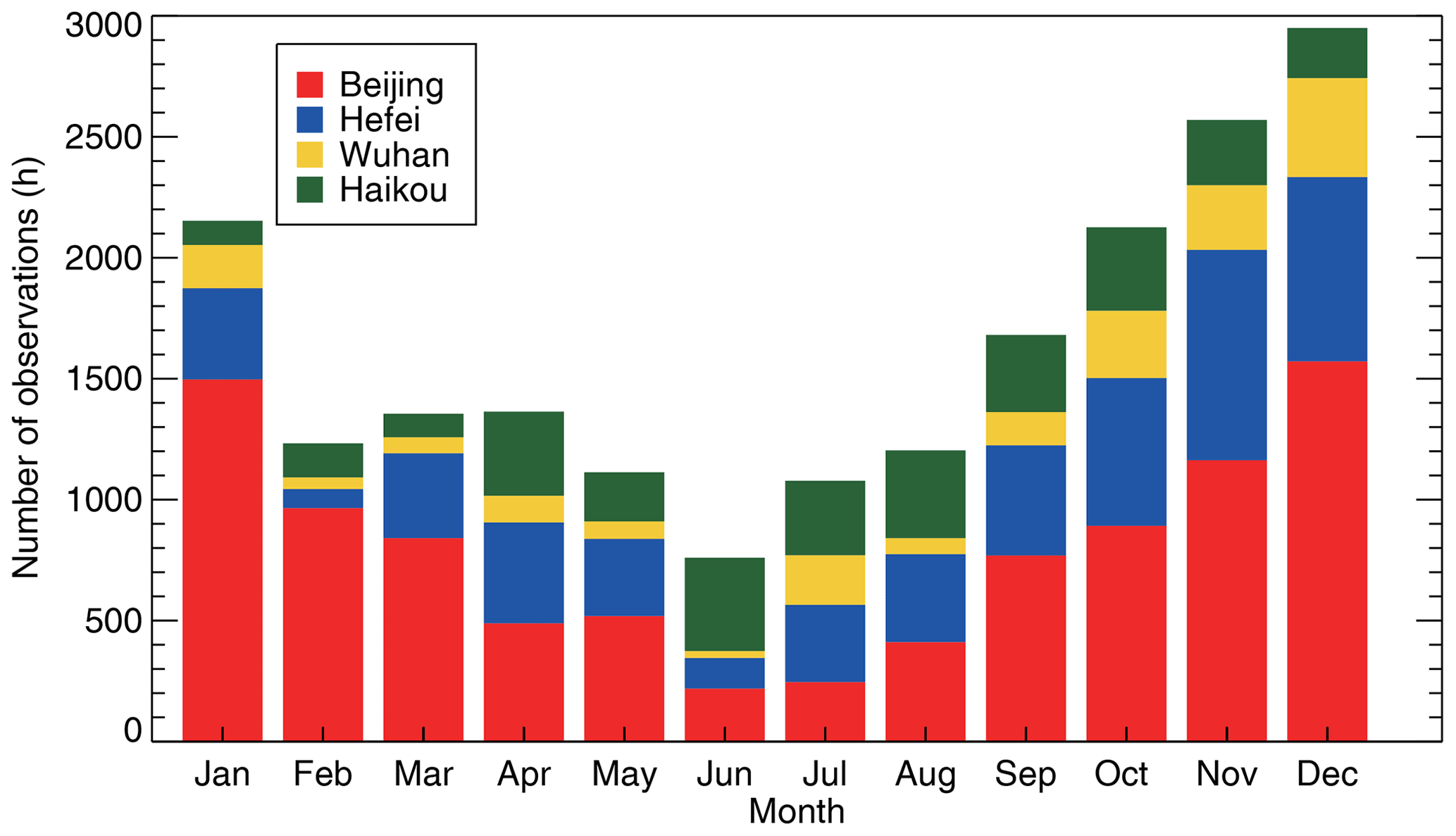
Figure 1Monthly distribution of the number of Na observations measured by the four Na lidars during the period 2005 to 2021.
Table 1Na lidar measurements and main parameters of the Na lidars.

2.2 Odin satellite
Odin is a limb-scanning satellite co-funded by Sweden, Canada, France, and Finland (Murtagh et al., 2002). On 20 February 2001, the satellite was launched from Svobodny, Russia. It is in a sun-synchronous orbit at approximately 600 km, with a descending node at 06:00 local time (LT) and an ascending node at 18:00 LT. The satellite conducts limb scans from 10 to 110 km altitude. The OSIRIS spectrometer is one of the two main instruments onboard (Llewellyn et al., 2004). The instrument measures radiance from the limb at wavelengths between 280 and 800 nm. The profiles of mesospheric Na number density have been retrieved from the limb-scanning measurements of the Na D dayglow at 589 nm with an altitude resolution of 2 km (Gumbel et al., 2007; Hedin and Gumbel, 2011), using an optimal estimation method (Rodgers, 2000). Figure 2 shows the time–latitude distribution of the number of the Na observations from OSIRIS during 2004–2009, using a 5 d × 5∘ latitude grid as a resolution. The satellite orbits do not fully cover latitudes greater than 85∘. Furthermore, mesospheric dayglow measurements cannot be made at mid- to high-latitudes in the winter hemisphere, due to the lack of daylight when the solar zenith angle is larger than 92∘. Therefore, the ground-based Na lidars, in addition to OSIRIS limb-scanning radiance measurements, provide an important measurement of local Na layers, notably in filling in data gaps during the winter.
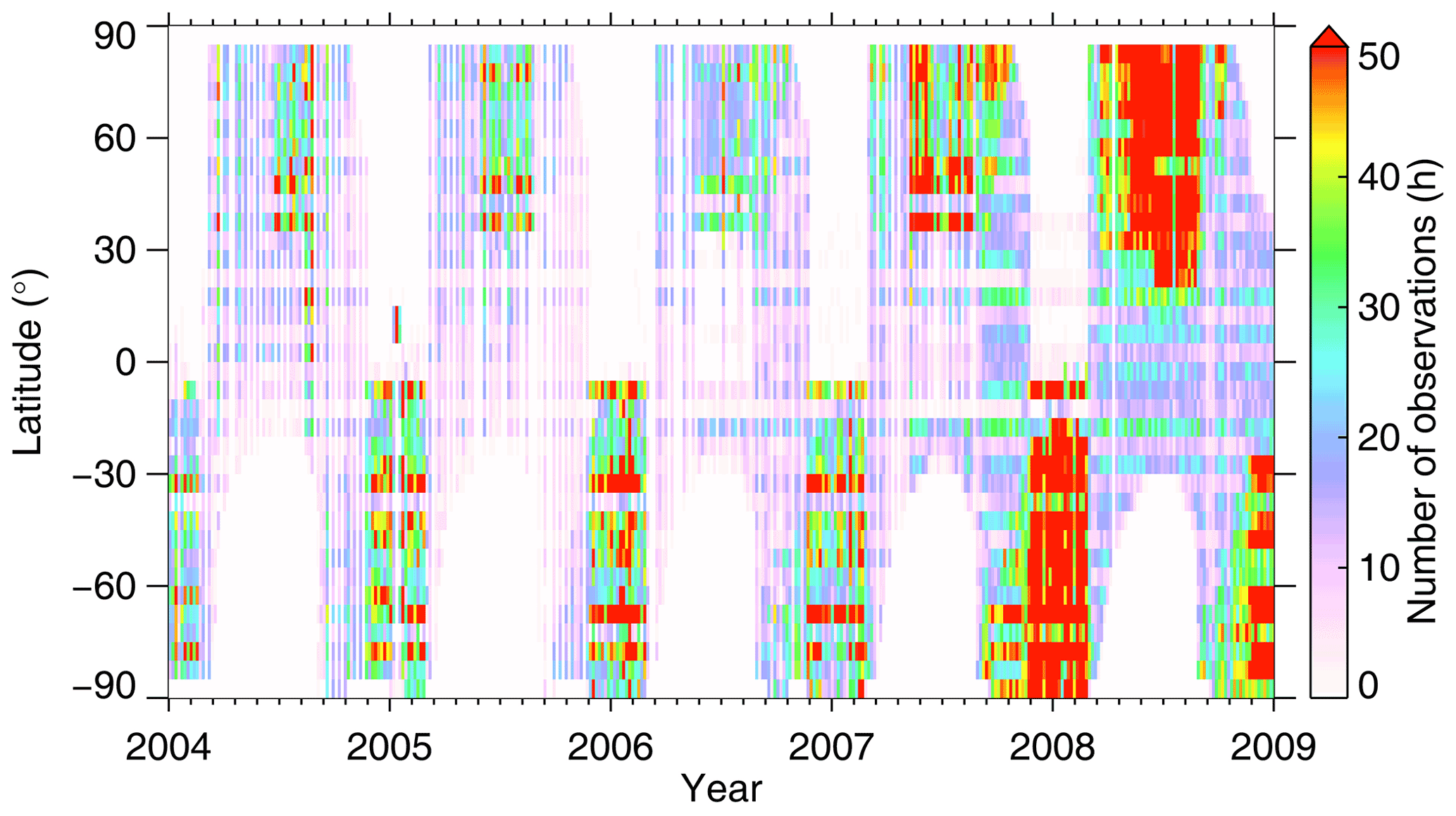
Figure 2Time–latitude distribution of the number of the OSIRIS limb-scanning radiance measurements made by the Odin satellite during the period 2004 to 2009, with a resolution of a 5 d × 5∘ latitude grid.
2.3 WACCM–Na
A global atmospheric model of the meteoric metals Fe, Na, K, Si, Ca, Al, Mg, and Ni (e.g. Feng et al., 2013; Marsh et al., 2013; Plane et al., 2014; Langowski et al., 2015; Plane et al., 2016, 2018; Daly et al., 2020; Plane et al., 2021) has been developed in order to advance understanding the meteor astronomy, atmospheric chemistry, and transport processes that control the different metal layers in the MLT (Feng et al., 2015; Plane et al., 2015; Wu et al., 2019). The model uses a seasonally varying meteoric injection rate of these metals at different latitudes and altitudes. In the present paper, we use a version of WACCM–Na (Marsh et al., 2013) nudged with NASA's Modern-Era Retrospective Analysis for Research and Applications (MERRA2) (Molod et al., 2015). Here we run the model with a very high vertical resolution (144 vertical levels) of ∼ 500 m in the MLT (e.g. Yuan et al., 2019); and the horizontal resolution is 1.9∘ in latitude by 2.5∘ in longitude. The model run covers the time period from January 2004 to the end of 2009. Here we sampled the model output every 30 min for the locations of the CMP lidar stations. The simulated Na number density is then used to compare with the observations from the Odin satellite and the Na lidars.
2.4 COSMIC radio occultation
There is strong evidence for close coupling between the metal layers and ionospheric Es layers (Xue et al., 2017). Es layers are thin layers of highly concentrated plasma composed of metallic ions and electrons that occur between 90–130 km altitude. At mid-latitudes they are caused by the vertical convergence of ions at the null points of wind shears (Whitehead, 1960; Davis and Johnson, 2005; Chu et al., 2014; Yu et al., 2021c). Strong plasma irregularities have a considerable impact on the amplitude and phase of radio occultation (RO) signals from the global navigation satellite system (GNSS) (Yue et al., 2015, 2016). Therefore, the ionospheric effects on GNSS RO signals can be used to investigate the global ionosphere's morphology. The GNSS RO data from the Constellation Observing System for Meteorology, Ionosphere and Climate (COSMIC) satellites during 2006–2014 have been used to study Es layers (Yu et al., 2020). The amplitude scintillation S4 index is defined as the standard deviation of the normalized intensity in GNSS RO signals. Large S4 values indicate the ionospheric irregularities with strong fluctuations in plasma density (Yue et al., 2015; Tsai et al., 2018). S4max is proportional to the critical frequency of the Es layer, with approximately 30.22 % and 69.57 % coincident measurements from RO and ground-based ionosondes having a relative difference less than 10 % and 30 %, respectively (Yu et al., 2021b). The maximum S4 index occurring between 90–130 km can be used as a proxy for the intensity of an Es layer (Yu et al., 2019b; L. Qiu et al., 2021). In the present study we also look into the climatology and seasonal variability of metallic ions within the Es layers, and the link between Es layers, the Na layer, and the presence of SSLs at low- and mid-latitudes.
3.1 Global map of Na layer
Figure 3 shows the time–latitude distribution of the Na column number density from the OSIRIS limb-scanning radiance measurements between 2004 and 2009, with a resolution of 5 d × 5∘ latitude grid. The Na column density is zonally averaged and integrated from 76 to 106 km altitude. Grey-shaded areas represent regions where OSIRIS limb-scanning radiance measurements were not made in winter. The time–latitude distribution of the Na column number density from OSIRIS shows a distinct annual cycle of the Na column density at mid- and high-latitudes, which is consistent with previous ground-based and satellite measurements (Plane et al., 1999; Fan et al., 2007b; Li et al., 2018). At latitudes between 30 and 90∘, the annual variation in Na column density becomes very significant. The maximum Na column density during winter is approximately 6×109 cm−2, and the summer minimum is approximately 1×109 cm−2. At low latitudes between 0 and 30∘, a small semi-annual variation in the column abundance in seen with maxima of 5×109 cm−2 in May and October. The stellar occultation measurements made by the GOMOS instrument onboard the Envisat satellite also showed a clear semi-annual oscillation in Na vertical column density at low latitudes that merges into an annual variation above 30∘ latitude (Fussen et al., 2010; Langowski et al., 2017). In the present study, the latitude dependence of the seasonal variation in the Na layer from the meridional chain of the CMP Na lidars is discussed in Sect. 3.2.
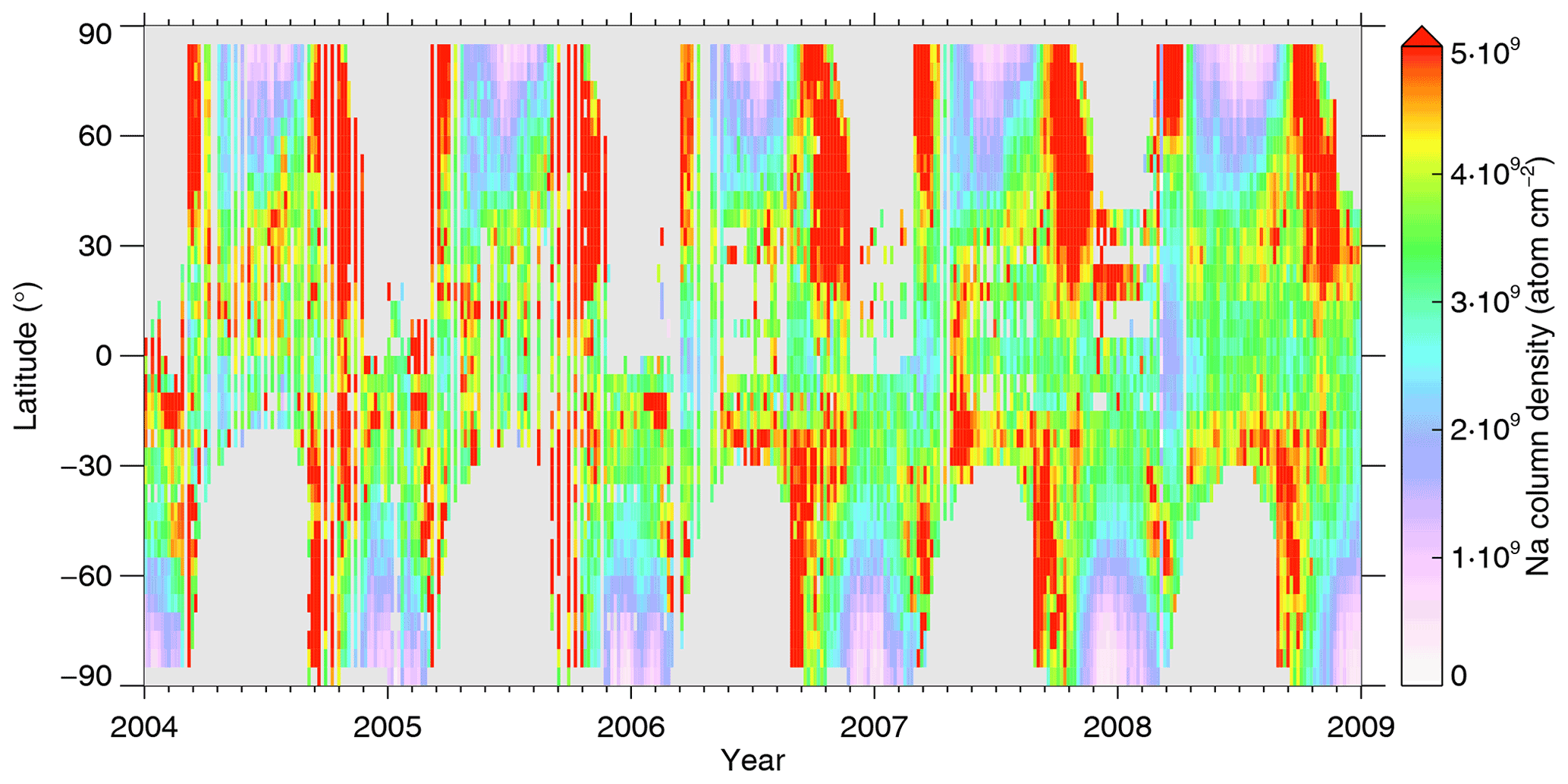
Figure 3Time–latitude distribution of the Na column number density from the OSIRIS limb-scanning radiance measurements made by the Odin satellite, with a resolution of a 5 d × 5∘ latitude grid. Na column density is integrated from 70 to 120 km altitude. Grey-shaded areas indicate the regions where OSIRIS limb-scanning radiance measurements were not made in winter.
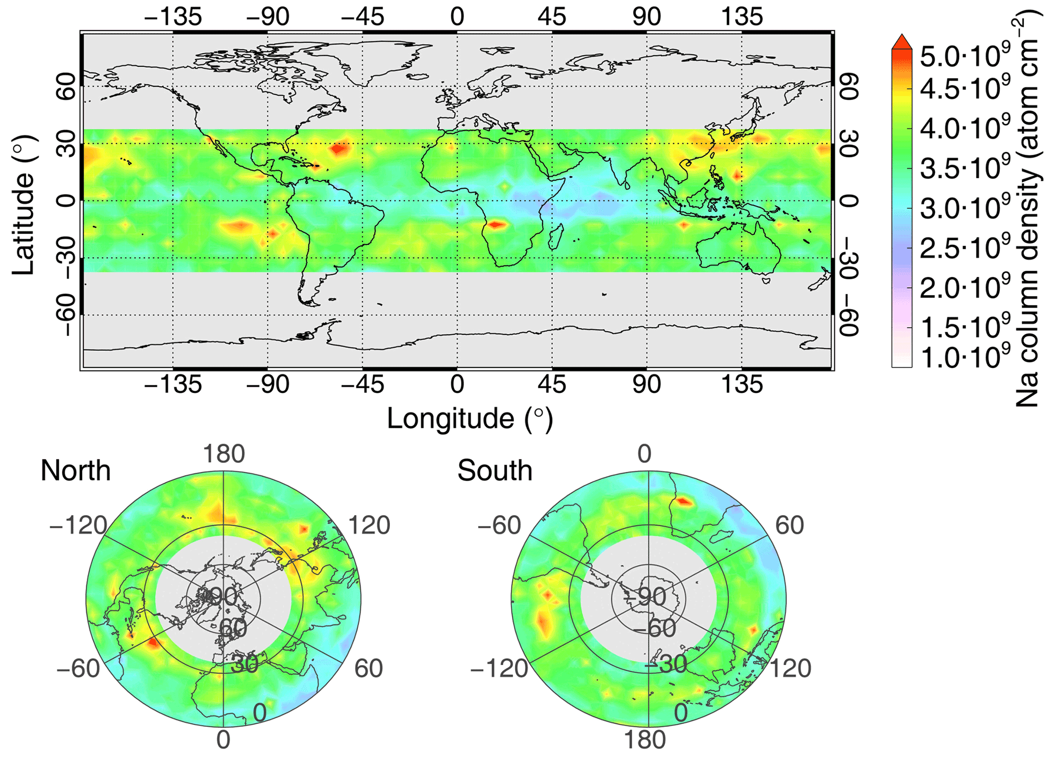
Figure 4Geographical distribution of the annual mean Na column number density below 40∘ latitude from the OSIRIS limb-scanning radiance measurements made by the Odin satellite during the period 2004 to 2009, with a spatial resolution of a 5∘ × 5∘ grid. Grey shading indicates the regions where there are no measurements or not enough measurements at mid- and high-latitudes in winter to calculate the annual average.
Figure 4 shows the geographical distribution of the annual mean Na column number density at latitudes below 40∘ in a 5∘ × 5∘ grid, based on the 6-year OSIRIS measurements from 2004 to 2009. As in Fig. 3, grey shading indicates the region where there are no measurements or not enough measurements at mid- to high-latitudes in winter to calculate the annual average. The annual average Na column at low-latitudes peaks in two broad bands between 10–40∘ N and S, with pronounced areas of high concentration over eastern Asia (90∘ E–140∘ E) and the north Pacific (140∘ E–150∘ W), the north Atlantic (50–80∘ W), and the south Pacific (80–115∘ W) and south Atlantic (0–45∘W). This geographical distribution is fairly consistent with the distribution of Es layers reported by Yu et al. (2019b). The observations of the Na layers have been made in most of these regions using ground-based lidars at Arecibo, Puerto Rico (18.3∘ N, 67.0∘ W) (Cai et al., 2019b); Cerro Pachón, Chile (30.3∘ S, 70.7∘ W) (Liu et al., 2016); Uji, Japan (34.9∘ N, 135.8∘ E) (Suzuki et al., 2010); Beijing, China (40.5∘ N, 116.0∘ E) (Gong et al., 2013); Hefei, China (31.8∘ N, 117.3∘ E) (Dou et al., 2009); Wuhan, China (30.5∘ N, 114.4∘ E) (Yi et al., 2013); and Haikou, China (19.5∘ N, 109.1∘ E) (Jiao et al., 2017). The limb-scanning radiance data from OSIRIS provide a near-global view of Na layers. However, because the peak Na density was not observed during the dark winter months, the annual mean Na column abundances at high latitudes from OSIRIS cannot be made.
The maps in Fig. 5 show the global distributions of the Na number column density from OSIRIS for four different seasons in a 5∘ × 5∘ grid. The Na layer clearly shows a global seasonal dependence with a pronounced minimum in the summer hemisphere. The Na column density at high latitudes reaches over 5×109 cm−2 in autumn and winter, and decreases to 1×109 cm−2 in summer. High concentration above 4.5×109 cm−2 in all four seasons can be seen over eastern Asia and the north Pacific, the north Atlantic, and the south Pacific and south Atlantic. Note that grey-shaded areas represent areas where OSIRIS limb-scanning radiance measurements were not made during the winter at high latitudes. On the other hand, the ground-based lidar measurements are a supplement to satellite data sets when the high-latitude Na layers are not solar-illuminated in winter. The Na column density has a maximum in winter from several local ground-based observations (Gibson and Sandford, 1971; Plane et al., 1999; She et al., 2000; Gardner et al., 2005; Yuan et al., 2012; Li et al., 2018; Andrioli et al., 2020) and global modelling studies of meteoric Na in the MLT (Marsh et al., 2013; Wu et al., 2021). The lower panels during each season depict the northern and southern polar views of the Na column density, and these views make the summer minimum in the high-latitude Na layers clearer. The significant summer-time depletion of high-latitude Na layers is primarily attributed to the temperature dependence of neutral Na chemistry with the very low temperature at the summer mesopause because of dramatic adiabatic cooling of upwelling air (Plane, 2003) and secondarily attributed to efficient removal of metallic species on noctilucent cloud particles (Plane et al., 2004; Raizada et al., 2007; Plane, 2012).
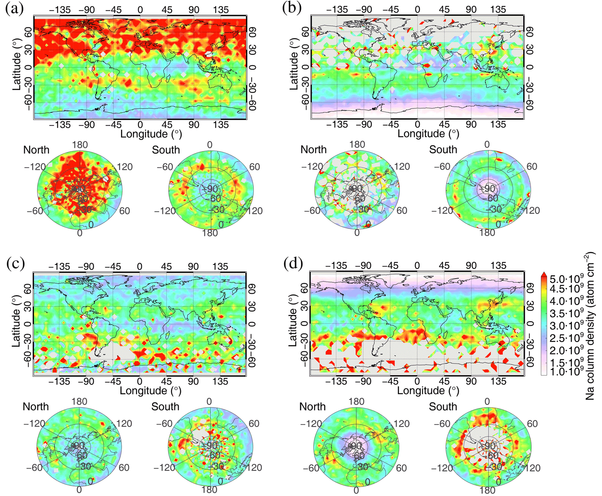
Figure 5Seasonal variations in the Na column number density from the OSIRIS limb-scanning radiance measurements made by the Odin satellite during the period 2004 to 2009, with a spatial resolution of a 5∘ × 5∘ grid. Maps for (a) autumn (September, October, November), (b) winter (December, January, February), (c) spring (March, April, May), and (d) summer (June, July, August). It is worth emphasising that the grey-shaded areas represent the areas where the OSIRIS limb-scanning radiance measurements were not made during the dark winter months at high latitudes, but these areas should have a winter maximum of Na column number density as indicated by the seasonal variations in Na layers from the ground-based lidar observations.
To compare with the OSIRIS results, the global map of the annual mean Na column number density simulated by WACCM–Na from 2004 to 2009 is shown in Fig. 6. The WACCM simulated Na column density ranges from 3.0×10⁹ to 4.6×109 cm−2. The largest Na column densities are seen at 60∘ S high-latitude, where the column density is 4.7×109 cm−2. In the tropics, the Na column is relatively small around 3.0×109 cm−2. The WACCM–Na model prediction has been shown in good agreement with the Na column density measured by the mid-latitude lidar at Fort Collins (41∘ N, 105∘ W) and the lidar at the South Pole (Marsh et al., 2013).
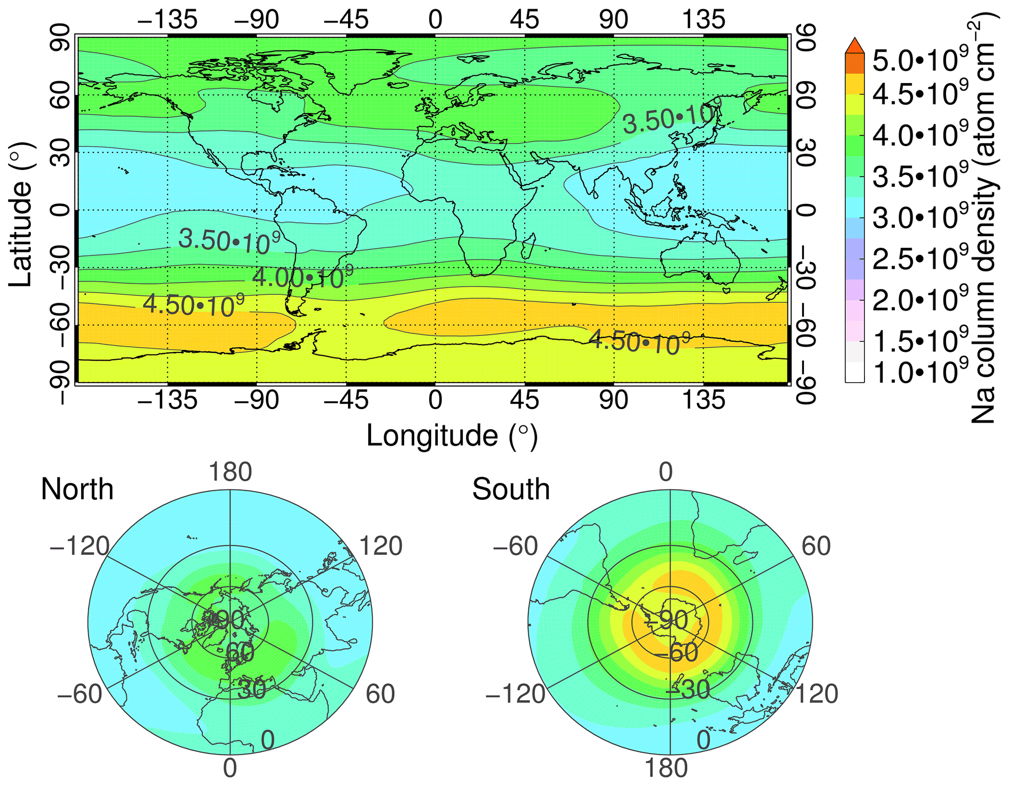
Figure 6Global geographical distribution of the annual mean WACCM simulated Na column number density during the period 2004 to 2009.
The maps in Fig. 7 show the global distributions of the WACCM simulated Na column density for four different seasons during the period 2004–2009. The Na column density in WACCM–Na shows a similar seasonal variation to the OSIRIS observations in Fig. 5. At high latitudes, the summer minimum is around 2.0×109 cm−2 in the WACCM–Na model, which is consistent with the measurements from OSIRIS in summer. The winter maximum in WACCM–Na is 5.0×109 cm−2 at high latitudes. However, the areas of pronounced Na column density observed from OSIRIS shown in Figs. 4–5, e.g. in eastern Asia and the north Atlantic, are not reproduced in the WACCM–Na simulations. In the following section, the ground-based measurements of Na layers from four lidars in the CMP are compared to satellite observations and WACCM simulations.
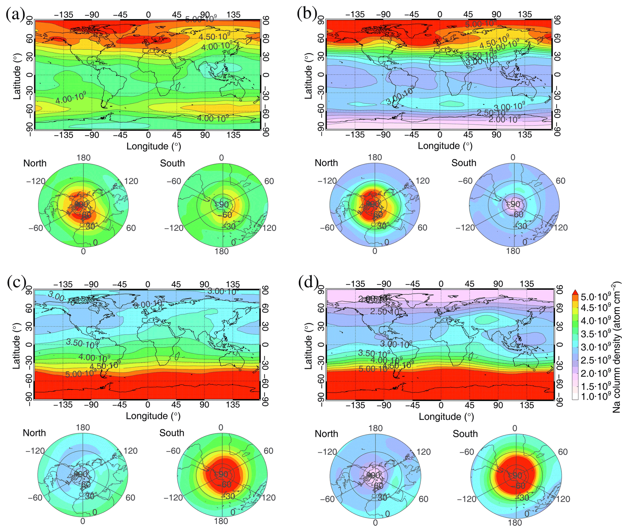
Figure 7Seasonal variations in the WACCM simulated Na column number density during the period 2004 to 2009. Maps for (a) autumn (September, October, November), (b) winter (December, January, February), (c) spring (March, April, May), and (d) summer (June, July, August).
3.2 Na layer from ground-based lidars, Odin satellite, and WACCM–Na model
Figure 8 shows the time series of mean Na number density profiles in a 5 d × 2 km average grid from the Na lidars at Beijing (40.5∘ N, 116.0∘ E), Hefei (31.8∘ N, 117.3∘ E), Wuhan (30.5∘ N, 114.4∘ E), and Haikou (19.5∘ N, 109.1∘ E). The lidar measurements at the four stations, particularly at the Beijing and Hefei mid-latitude stations, show an annual variation in Na layers with a winter maximum (Fig. 8a–b). There are over 9000 and 5000 h observations of the Na layer at Beijing and Hefei, respectively, and more than 1800 h at the other two stations.
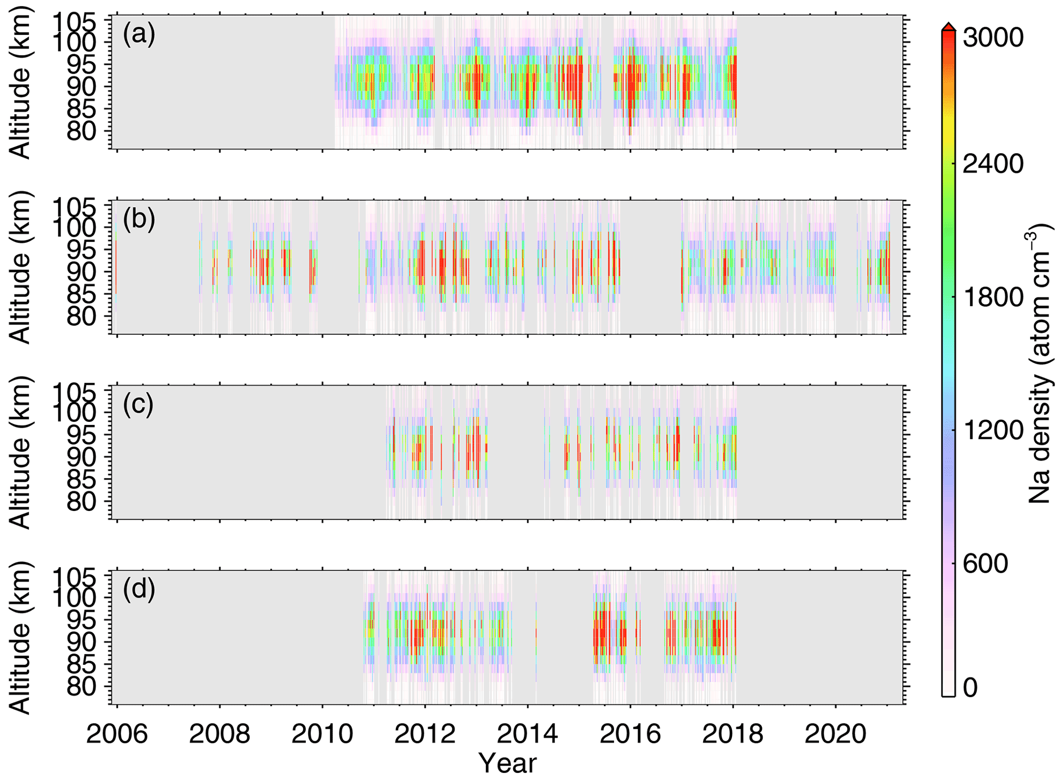
Figure 8Time series of mean Na number density in a 5 d × 2 km average grid from Na lidars at (a) Beijing (40.5∘ N, 116.0∘ E), (b) Hefei (31.8∘ N, 117.3∘ E), (c) Wuhan (30.5∘ N, 114.4∘ E), and (d) Haikou (19.5∘ N, 109.1∘ E).
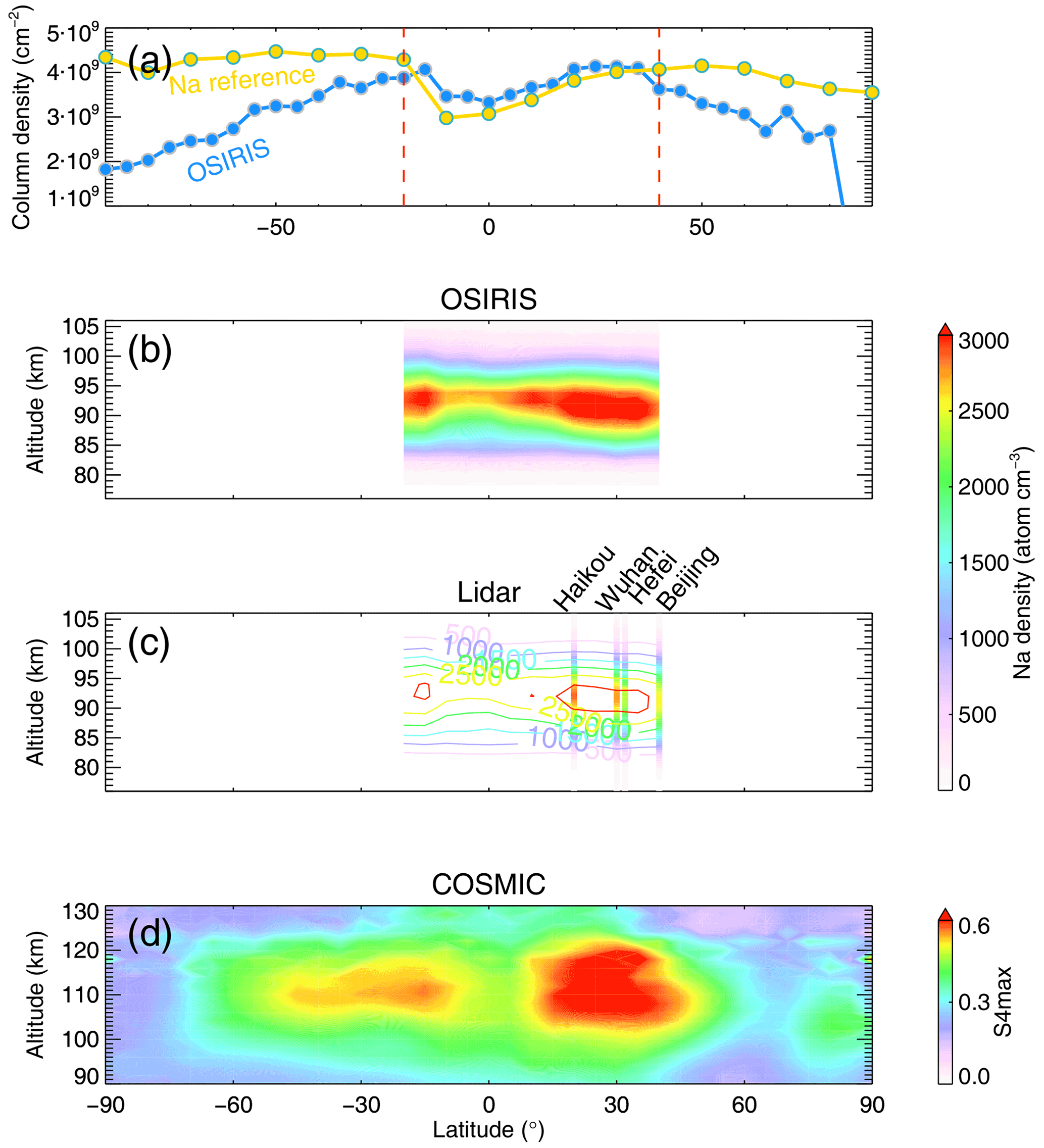
Figure 9(a) Annual mean Na column density from OSIRIS and Na reference by Plane (2022). Height–latitude distribution of the neutral Na layers and metallic ions: (b) Na number density from OSIRIS between 20∘ S and 40∘ N latitudes; (c) height-dependent Na density from the lidars at Beijing (40.5∘ N), Hefei (31.8∘ N), Wuhan (30.5∘ N), and Haikou (19.5∘ N), with superposed contour lines of Na number density from OSIRIS; and (d) Es layers represented by the S4max from COSMIC satellites.
Figure 9a shows the comparison of annual mean Na column density between OSIRIS measurements and Na reference by Plane (2022). The Na reference consists of zonally averaged Na climatology in 10∘ latitude bins. Good agreement is found between 20∘ S and 40∘ N latitudes. However, the annual mean OSIRIS at higher latitudes is largely underestimated due to few measurements in winter. Therefore, the height–latitude distributions of the neutral Na layer from OSIRIS between 20∘S and 40∘ N latitudes, and Na lidars are shown in Fig. 9b and c. In Fig. 9b, the annual mean Na number density from OSIRIS shows a northern number density over 3000 cm−3 at 10–40∘ N latitudes and a southern density over 3000 cm−3 at 15∘ S latitude. Figure 9c shows the height dependent Na density from the lidars at Beijing (40.5∘ N), Hefei (31.8∘ N), Wuhan (30.5∘ N), and Haikou (19.5∘ N), along with superposed contour lines of Na number density from OSIRIS. The peak number density of Na layers at the four stations is between 2500 and 3000 cm−3, in accord with the observations from OSIRIS. The low-latitude Na layer at Haikou has a relatively higher peak density of nearly 2900 cm−3 than the mid-latitude Na layers at Hefei and Beijing with the peak density of 2500–2550 cm−3. The Na layer at Wuhan has a moderate peak density of approximately 2750 cm−3. The Na number densities at the four lidar stations agree well with the latitudinal variation in the Na number density observed from OSIRIS. A large Na column density in eastern Asia at 10–40∘ N latitude can also be found in the global map of the Na layer from OSIRIS over four seasons (Figs. 4 and 5), which is not reproduced by WACCM–Na (Figs. 6 and 7).
More recently, the distribution of Mg+ column density simulated by WACCM–X (Wu et al., 2021) shows a stronger convergence along the magnetic equator. The equatorial metallic ions are uplifted by V×B forcing and drift down along the magnetic field lines to the subtropical region. The transport of metallic ions is generally consistent with the fountain effect, and the fountain effect is stronger over east Asia (Wu et al., 2021). The metal layer can be influenced by the metallic ions as the major reservoir of the neutrals through the recombination between ions and electrons, though the neutral atoms are not directly transported by the electromagnetic field (Cai et al., 2019a). The electrodynamical transport of metallic ions has an important impact on the global distribution of metal ions and atoms (Wu et al., 2021). It could explain why WACCM–Na does not capture the large Na observed by the CMP lidars at 10–40∘ N.
Figure 9d shows the height–latitude distribution of Es layers represented by the S4max from COSMIC satellites. The latitude distribution of Es layers show a north–south hemisphere asymmetry. There is a broad maximum between 10 and 40∘ N in the Northern Hemisphere and a smaller peak distribution around 15∘S latitude in the Southern Hemisphere. A small enhancement of the Es layer intensity can be found at 75–90∘ N northern high latitudes.
It is an interesting feature that both the neutral Na layer and Es layer intensity have a similar latitude distribution (at least below 40∘ N latitude). Many previous studies have shown a strong correlation between local SSLs and Es layers (Dou et al., 2010; Kane et al., 2001; Sarkhel et al., 2012; Dou et al., 2013). The neutralization of metallic ions is the most commonly accepted mechanism for SSL formation (Cox and Plane, 1998). Na layer and Es layers both have a prominent seasonal variation. Na layer has a maximum density in winter and the Es layers have a maximum density in summer. The geographical distributions of Na atoms and metallic ions with Es layers, particularly the similar pronounced areas of high concentration, should be related. Therefore, it indicates that it is necessary to incorporate the electrodynamical transport of metallic ions within Es layers into a global model of Na.
Previous ground-based measurements at 51∘ N (Gibson and Sandford, 1971), 41∘ N (She et al., 2000; Yuan et al., 2012), 23∘ S (Andrioli et al., 2020), and 90∘S (Gardner et al., 2005) have reported that the Na layers display a seasonal variation at latitudes greater than 20∘. A semi-annual oscillation in the Na layer was found from the recent lidar observations in the Southern Hemisphere from a dual Na/K Na lidar at São José dos Campos (23.1∘ S, 45.9∘ W), Brazil (Andrioli et al., 2020), in which the seasonal variation in meteor ablations can not account for the semi-annual behaviour of Na layers.
For further comparison with the CMP Na lidar observations, the measurements of Na layers from OSIRIS made within a region of ±5∘ latitude and longitude square centred on each ground-based lidar station were used. The measurements of Na number density in the morning from OSIRIS at about 06:00 LT (descending node) are compared with the ground-based observations from Na lidars at 04:00–06:00 LT. The measurements in the evening from OSIRIS at about 18:00 LT (ascending node) are compared with the observations from Na lidars at 18:00–20:00 LT.
3.3 Seasonal variation
Figure 10 shows the monthly variations in Na number density in the morning from OSIRIS at about 06:00 LT (descending node) and the Na lidars at 04:00–06:00 LT at Beijing, Hefei, Wuhan, and Haikou. The Na number densities from OSIRIS and Na lidar both show a significant seasonal variation at Beijing in Fig. 10a and b. The Na number density from OSIRIS shows a larger summer minimum of 2000 cm−3 with the standard error of 200 cm−3 in June and a winter maximum of 5300 cm−3 with the standard error of 300 cm−3 in October than that from the Na lidar with a summer minimum of 1800±200 cm−3 in July and a winter maximum of 3300±100 cm−3 in December. The standard error is calculated from the standard deviation of monthly mean divided by the square root of the number of points in each month. Figure 10c and d show Na number density from OSIRIS and Na lidar at Hefei. The summer depletion of the Na layer is observed at Hefei from lidar, with a minimum of 1700±100 cm−3 in July. The maximum Na density in winter at Hefei is 3100±100 cm−3 in November from Na lidar and 5000±400 cm−3 in October from OSIRIS. The depletion of the relatively low-latitude Na density in summer is not significant at Wuhan and Haikou, and the Na layers show a semiannual variation with peaks at equinox from the Na lidars. In Fig. 10f, the winter maximum from Na lidar at Wuhan is 4100±300 cm−3 in January, and the secondary peaks are 3000±300 cm−3 in April and 3700±200 cm−3 in November. In Fig. 10h, the peaks are 4300±200 cm−3 in October and 3400±300 cm−3 in March. In Fig. 10e and g, the Na number densities from OSIRIS show an annual variation with maxima of 5400±400 and 5600±700 cm−3 at Wuhan and Haikou in October. The Na number density from OSIRIS is generally larger than that from Na lidars at the four stations.
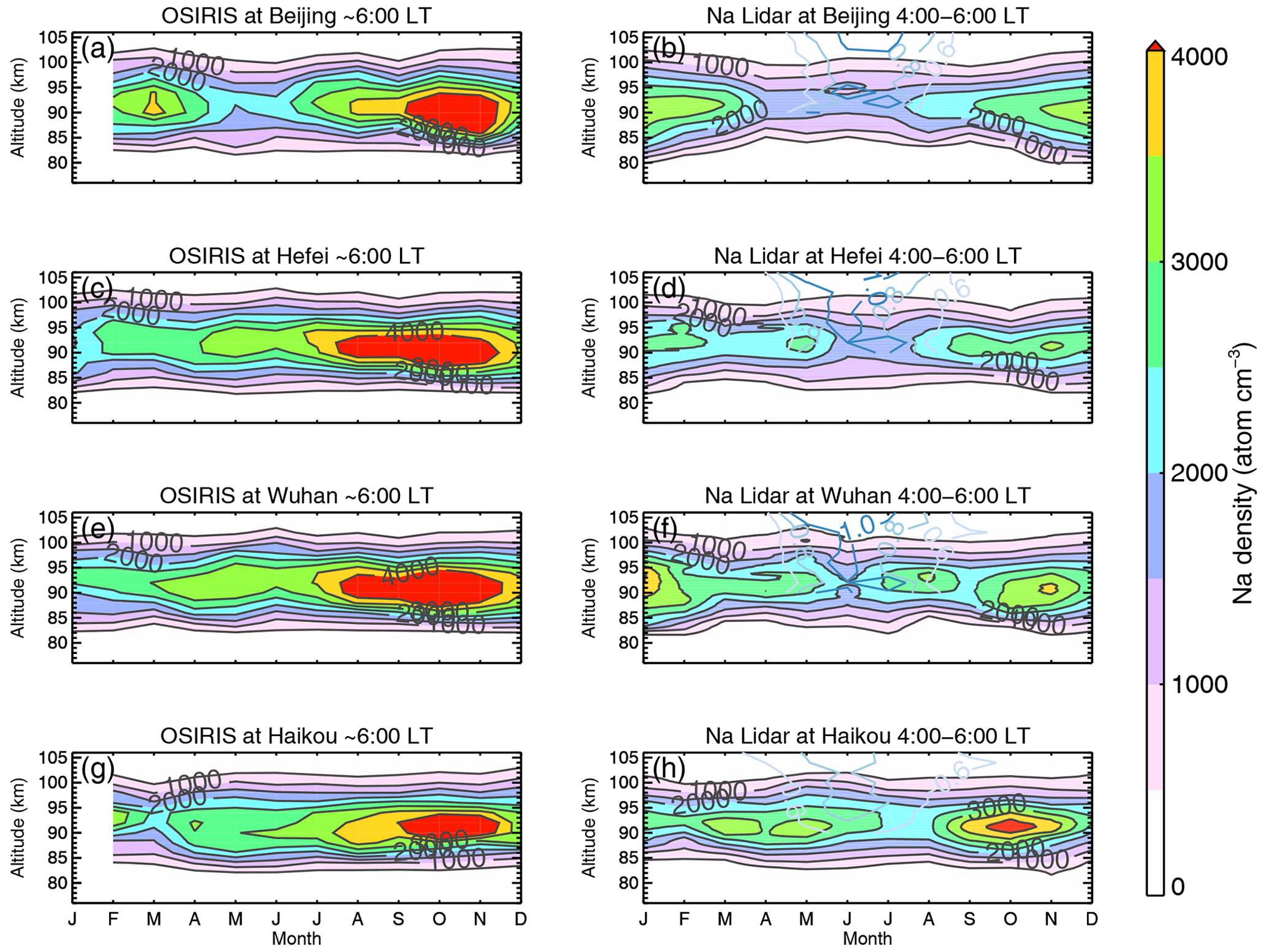
Figure 10Comparisons of monthly mean of Na number density in the morning, from OSIRIS at about 06:00 LT (descending node) and Na lidars at 04:00–06:00 LT (a–b) at Beijing, (c–d) Hefei, (e–f) Wuhan, and (g–h) Haikou. The summer maximum Es layers represented by S4max at levels of 0.6, 0.8, and 1.0 are shown as light to dark blue contour lines, superposed on the Na density contour from lidars on the right panels.
On the right panels of Fig. 10, the peak densities of the Es layers in summer are superimposed on the Na density contour from lidars, represented by the S4max at levels of 0.6, 0.8, and 1.0 as the light to dark blue contour lines. The response of the Na layer to the strong Es layers in summer is not very significant. Even though the density of the Na layer is lowest in summer because of the very low temperature at the mesopause, the Na layer can be influenced by the neutralization of metallic ions with a summer maximum of Es layers. It has been found that the sporadic enhanced Na layers in the upper mesosphere and thermosphere occur more frequently in summer than around the equinoxes, which are generally associated with the presence of the Es layer (Dou et al., 2013). The sudden enhancement of neutral metal density, which appears abruptly in a thin layer (full width at half maximum ∼1 km) on the topside of the normal metal layer (Clemesha, 1995), has a strong seasonal dependence with the highest occurrence rate in summer but it was rarely observed in other seasons (Qiu et al., 2016). Based on the observations from lidars and satellites, the analysis of the climatology and seasonal variations of the Es layers, the sporadic metal layers (SSLs for Na), and the Na layers is in the Discussion section.
Figure 11 shows the monthly variations in Na number density in the evening from OSIRIS at about 18:00 LT (ascending node) and Na lidars at 18:00–20:00 LT. Because the time of the ascending node shifted from 18:00 to 18:50 LT over the years, the number of Na density data in the evening, particularly in the equatorial region, is much less than that in the morning from the OSIRIS limb-scanning radiance measurements (Hedin and Gumbel, 2011). The Na number density in the evening is smaller than that in the morning. The Na number density from OSIRIS is generally larger than that from the Na lidars. In the right-hand panels of Fig. 11, the observations from the four lidars show a significant summer depletion of the Na layer. The observations from Na lidars show a shift from an annual variation in Na density at Beijing and Hefei to a semiannual variation at Wuhan and Haikou, which is consistent with the seasonal variation with latitude in Fig. 10. The Na number density minimum from lidars is around 1500 cm−3 in summer and the maximum density is around 2500 cm−3.
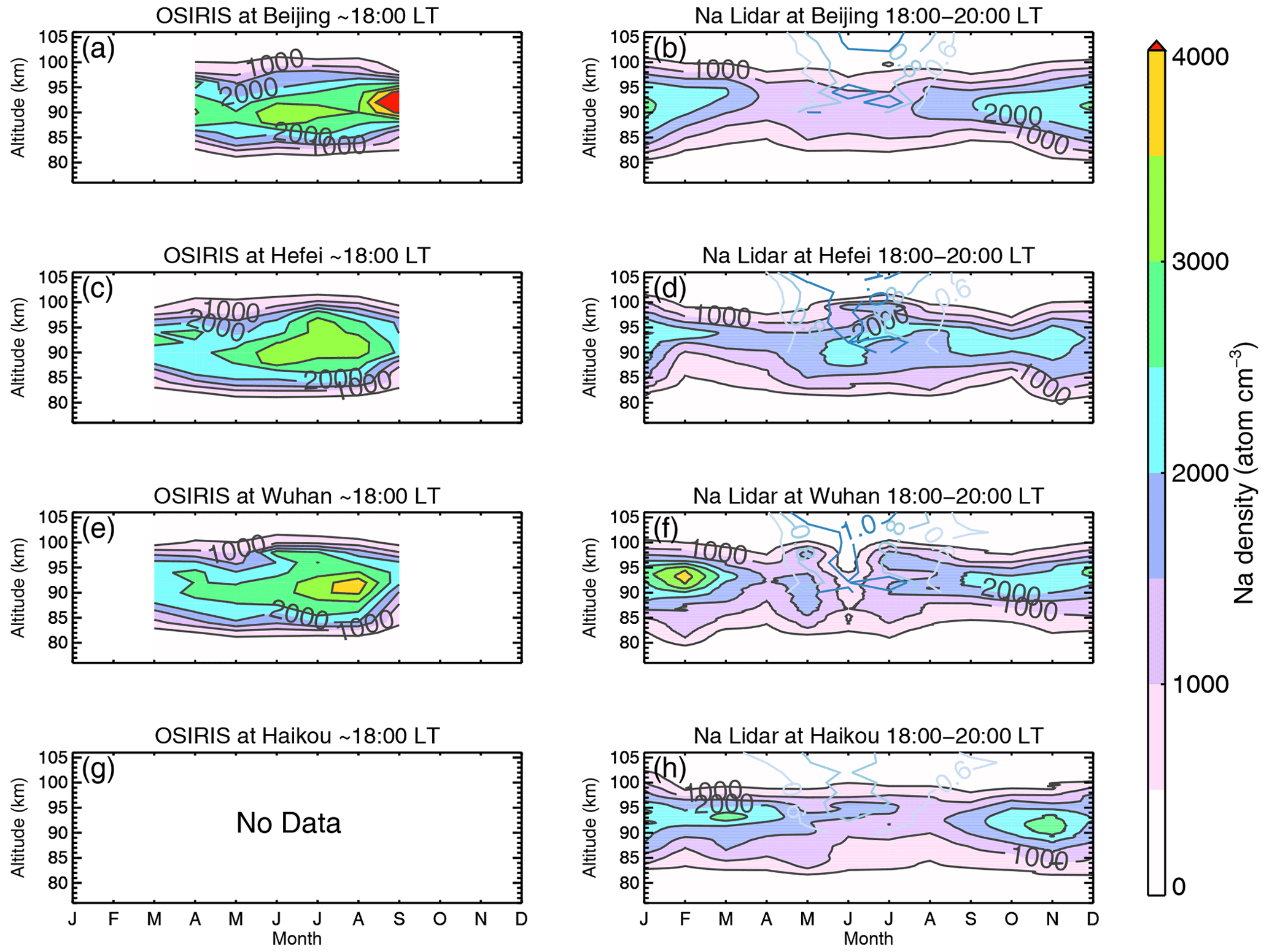
Figure 11Comparisons of monthly mean of Na number density in the evening, from OSIRIS at about 18:00 LT (ascending node) and Na lidars at 18:00–20:00 LT (a–b) at Beijing, (c–d) Hefei, (e–f) Wuhan, and (g–h) Haikou.
Figure 12 shows the monthly variations in the WACCM simulated Na number density at 06:00 LT in the morning and 18:00 LT in the evening. In general, WACCM–Na is capable of reproducing the seasonal variation in the Na layer. However, WACCM underestimates the seasonal variability of the Na layer as observed by lidars at Wuhan and Haikou. It may arise from the fact that the seasonal variability of vertical transport of atmospheric constituents modelled in WACCM is underestimated since the sub-grid gravity waves and turbulence fluctuations are unresolved with limited resolution, or the equatorial plasma fountain effect is not included in model. The vertical flux of Na atoms in the mesopause region employed in WACCM–Na is much smaller than that from lidar measurements (Marsh et al., 2013). The WACCM simulations at 06:00 LT show a peak Na number density of approximately 3000 cm−3 in October and a secondary peak of approximately 2500 cm−3 in March. The WACCM simulated Na density at 18:00 LT shows a similar variation. The peak density is approximately 3000 cm−3 in October, whereas the secondary peak in March is not significant.
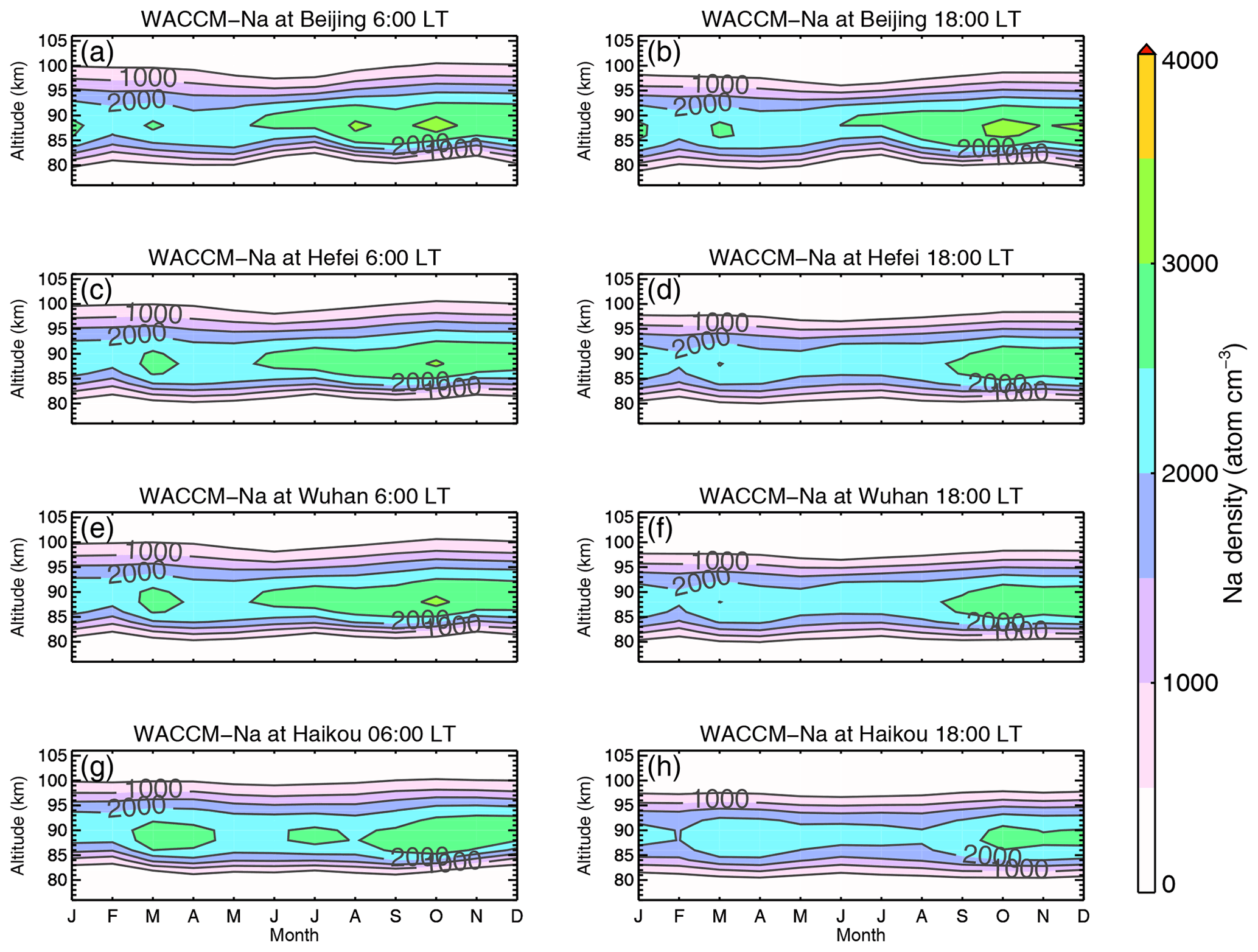
Figure 12Monthly mean of the WACCM simulated Na number density in the morning at 06:00 LT and in the evening at 18:00 LT (a–b) at Beijing, (c–d) Hefei, (e–f) Wuhan, and (g–h) Haikou.
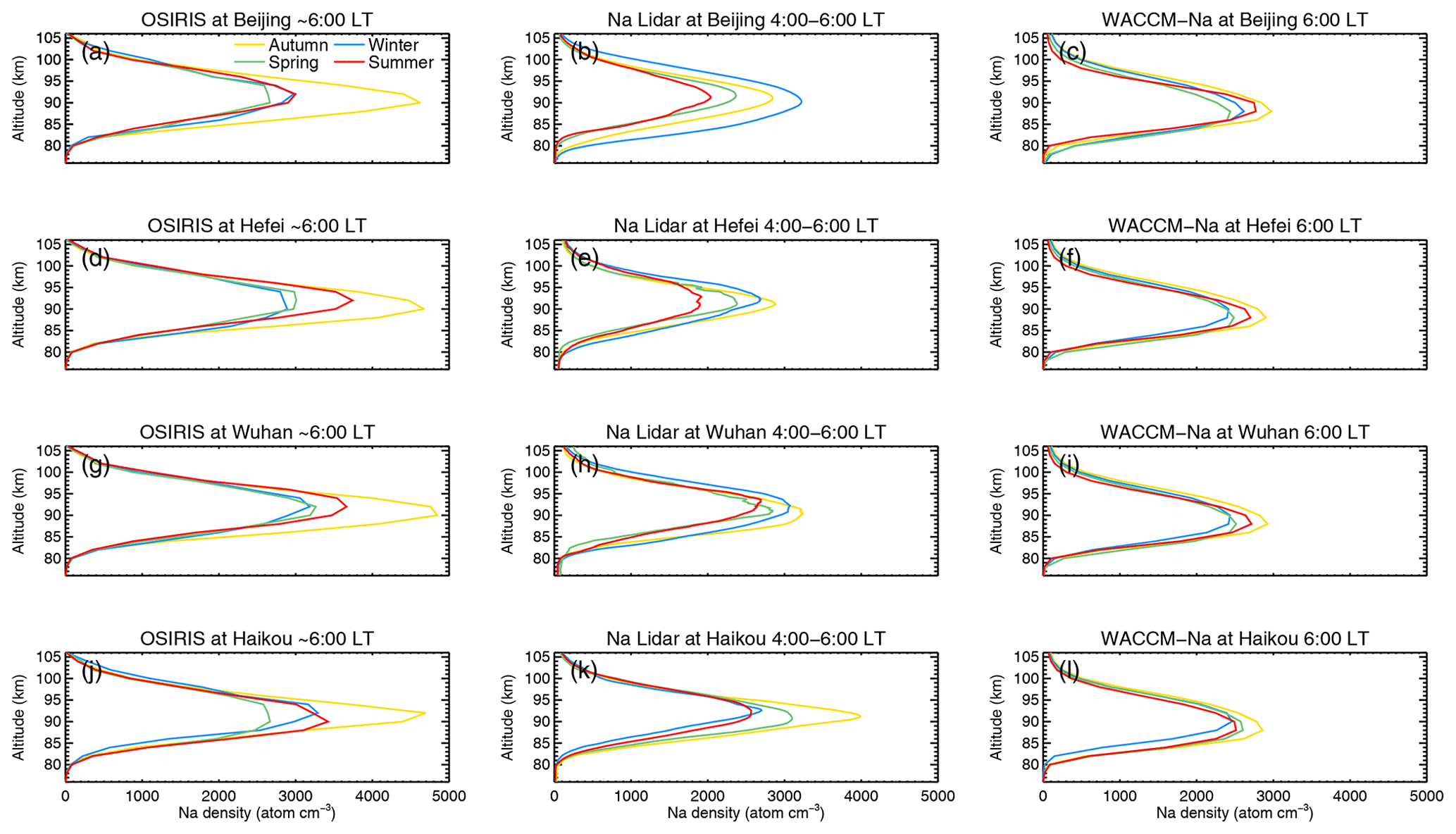
Figure 13Comparisons of seasonal Na number density profiles in the morning from OSIRIS at 06:00 LT, Na lidars at 04:00–06:00 LT, and WACCM–Na at 06:00 LT (a–c) at Beijing, (d–f) Hefei, (g–i) Wuhan, and (j–l) Haikou.
Figure 13 compares the seasonal profiles of Na number density in the morning from OSIRIS at 06:00 LT, Na lidars at 04:00–06:00 LT, and WACCM–Na at 06:00 LT at Beijing (panels a–c), Hefei (panels d–f), Wuhan (panels g–i), and Haikou (panels j–l). The left panels show the vertical profiles of Na number density from OSIRIS with a 2 km altitude resolution between 76 and 106 km, within a region of ±5∘ latitude and longitude square centred on each lidar station. Due to the absence of daylight when the solar zenith angle is larger than 92∘, there are fewer observations in winter than in the other three seasons. The observations from OSIRIS show similar seasonal mean vertical profiles of Na density as above the four lidar stations. The maximum Na density from OSIRIS is 4600–4900 cm−3 in autumn, with a peak height around 90 km. The peak density is 2700–3500 cm−3 during other seasons.
The seasonal profiles of Na number density from Na lidars at 04:00–06:00 LT are shown in the middle panels. In Fig. 13b, the Na layer at Beijing has a significant seasonal dependence, with the maximum Na density of approximately 3200 cm−3 in winter and a peak height of 91 km. In Fig. 13e, h, and k, the maximum Na density is 2900 cm−3 at Hefei, 3200 cm−3 at Wuhan, and 4000 cm−3 at Haikou in autumn, with a peak height of 91 km. Although the vertical resolution of the profiles of Na number density from OSIRIS limb-scanning radiance measurements is lower than that of ground-based Na lidars, the OSIRIS data are nevertheless in good agreement with the measurements from the Na lidars. The observations from the OSIRIS spectrometer on the Odin satellite therefore provide a reliable measurement of the Na layer. The right-hand panels show the seasonal profiles of Na number density simulated by WACCM–Na, which exhibit similar but weak seasonal profiles. The maximum Na density is 2800–3000 cm−3 in autumn, with a peak height of 88 km. The peak density is 2400–2500 cm−3 during the other seasons.
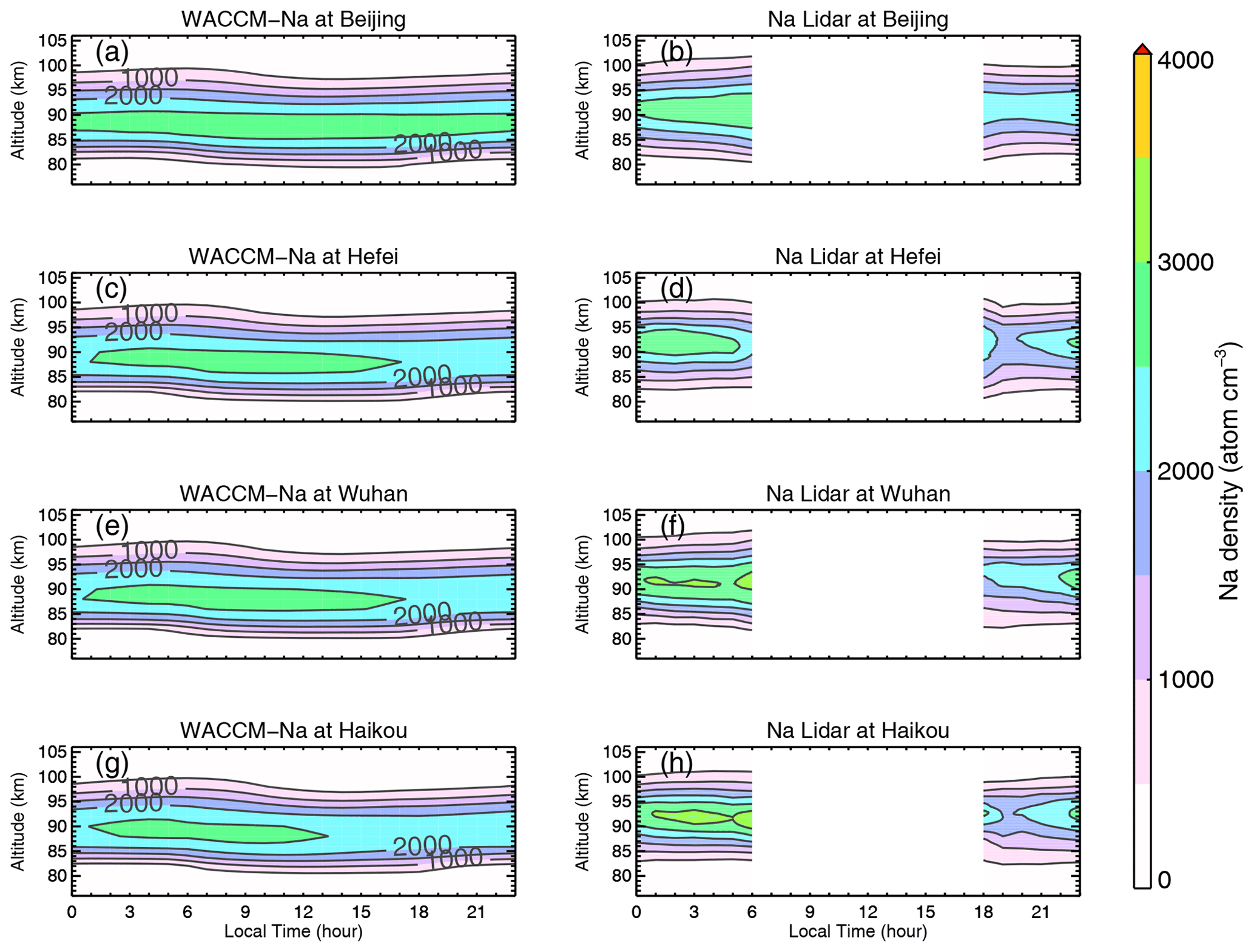
Figure 14Diurnal variations of the WACCM simulated Na number density and the lidar-observed nighttime Na number density (a–b) at Beijing, (c–d) at Hefei, (e–f) at Wuhan, and (g–h) at Haikou.
3.4 Diurnal variation
Figure 14 shows the full diurnal variation of the WACCM simulated Na number density and the lidar-observed nighttime Na number density. The Na layer is enhanced after midnight in the WACCM simulations. It is consistent with the observations from Na lidars that the morning Na density around 06:00 LT is 10 %–30 % larger than the evening Na density around 18:00 LT. After sunrise, an increase of Na density on the bottom side of the layer and removal of Na density on the topside of the layer can be found in WACCM simulations. Ion–molecule chemistry plays an important role in the Na layer above 96 km altitude (Cox and Plane, 1998). The influence of the odd oxygen (O and O3)/hydrogen (OH, HO2) chemistry and photochemistry of the major reservoir species (NaHCO3) dominates below 96 km altitude (Plane et al., 1999, 2015; Yuan et al., 2019; Xia et al., 2020). Due to the increased solar radiation and the increased NO+ and O ions, atomic Na is removed off the topside of the Na layer after sunrise and transformed to Na+. The photolysis of the main reservoir, NaHCO3, causes an increase in Na atoms on the bottom side of the layer after sunrise. WACCM also reproduces the diurnal variation in the Na layer driven by the diurnal tidal modulations (Liu et al., 2013; Yuan et al., 2014a). The right-hand panels of Fig. 14 show that lidar-measured Na density after midnight is larger than in the evening, in agreement with WACCM.
The global distribution of the Na layer is fairly consistent with the distribution of Es layers. Figure 15 shows the further analysis of the correlation between Es and SSL. The monthly variations in the climatology of Na column number density from OSIRIS and Na lidars, and the Es layer intensity represented by the S4max from COSMIC are compared to the monthly variations in the probability of SSL events observed by the four Na lidars in 2011/2012 reported in Dou et al. (2013). The dark and light green lines represent the monthly mean Na column number density from Na lidars and OSIRIS, respectively, with the standard errors of the mean represented by the width of the dark green bars and the light green shaded areas. The standard error was calculated from the standard deviations of the monthly mean divided by the square root of the number of points in each month. The orange and yellow bars in the histogram represent the monthly variations in the number of SSL nights and total nights measured by lidars. The orange line represents the probability of SSLs per day. The intensity of the Es layer at the height of 95–97 km is represented by the blue lines, with the standard errors represented by the width of the blue shaded areas.
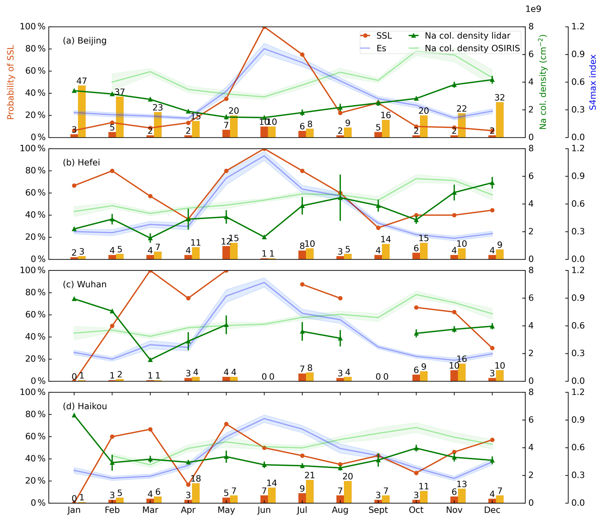
Figure 15Monthly variations in probability of SSLs per day (orange lines), Es layer intensity represented by S4max at the height of 95–97 km (blue lines), and Na column number density between 76 and 106 km from OSIRIS (light green lines) and Na lidars (dark green lines) in 2011/2012, at (a) Beijing, (b) Hefei, (c) Wuhan, and (d) Haikou. The orange and yellow bars in the histogram exhibit the number of SSL nights and total nights measured by lidars. The standard errors of the metallic ion density are represented by the width of the blue shaded area. The standard errors of the monthly Na column number density from OSIRIS and Na lidars are represented by the width of the light green shaded area and the dark green bars. The standard error was calculated from the standard deviations of monthly mean divided by the square root of the number of points in each month.
Figure 15a shows a strong correlation between Es layers (blue line) and SSLs (orange line) at Beijing, with a summer maximum and a winter minimum. The probability of SSLs can reach up to 100 % d−1 (10 SSL events out of 10 nights) in June, compared to approximately 6 % d−1 in December and January. The intensity of the Es layer is represented by the S4max index (Yu et al., 2019b, 2021b; L. Qiu et al., 2021). S4max is 0.96 in June, more than three times the value of 0.27–0.28 in December and January. Both the observations from OSIRIS and the Na lidar show an annual change in the Na column number density, with a summer minimum and a winter maximum. The SSLs are more correlated to Es layers at Beijing at a higher latitude compared to the other three stations. In Fig. 15b–d, the probability of SSLs shows a semi-annual variation at Hefei, Wuhan, and Haikou. The probability of SSLs reaches a peak in summer and reaches a secondary peak in February and March. The summer maximum occurrence of SSLs is consistent with the summer maximum intensity of the Es layer. The secondary peak in occurrence of SSLs in February and March is consistent with the climatology of Na layers from lidars. The correlation between the probability of SSLs and the density of Es layer at Haikou station in Fig. 15d is less significant than those at other three stations. The SSL formation could be related to the variations of Es layer, e.g. the winter-to-summer dynamical process of mid-latitude Es affected by the thermospheric meridional circulation at 95–115 km height (Yu et al., 2021c), and the low-latitude Es affected by the equatorial electrojet irregularities and the geomagnetic activity (Whitehead, 1970, 1989; Yu et al., 2021a).
The SSLs and the Es layer both occur more frequently in summer than in winter at the four lidar stations. The numerical simulations (Cai et al., 2019b) revealed that the distinct seasonal behaviours of the Es layer, the Na number density, and the width of the Na main layer strongly influence the seasonal occurrence of SSLs. Since the vertical shear of ion velocity is negative above 100 km in summer, it represents the generation of strong convergence of ions. The metallic ions are converged into thin Es layers that descend below 100 km under the influence of tides. Na+ can be easily neutralized through three-body reactions into SSLs. Besides, the Na column number density from OSIRIS and Na lidars is much lower in summer than in winter. A narrow main layer with a relatively low peak number density in summer makes an abrupt increase in the Na number density more apparent, and thus easy to be observed as an SSL.
We present a study on the climatology of Na layers at mid- and low-latitudes, from the ground-based measurements obtained from a lidar network of four Na fluorescence lidars along 120∘ E longitude in the CMP, the OSIRIS limb-scanning radiance measurements detected by the Odin satellite, and WACCM–Na simulations.
The geographical distribution of the Na layer shows a global seasonal dependence from OSIRIS measurements and WACCM model. The pronounced areas of high Na column density above 4.5 × 109 cm−2 can be seen over eastern Asia and the north Pacific, the north Atlantic, and the south Pacific and south Atlantic from OSIRIS in all four seasons. This geographical distribution is fairly consistent with the distribution of Es layers reported by Yu et al. (2019b).
Up to January 2021, the Na lidars at Beijing (40.5∘ N, 116.0∘ E), Hefei (31.8∘ N, 117.3∘ E), Wuhan (30.5∘ N, 114.4∘ E), and Haikou (19.5∘ N, 109.1∘ E) collected vertical profiles of Na density for a total of 2136 nights (19 587 h). Ground-based Na lidars can provide extremely high temporal and altitude resolution local observations of Na layers. However, the lidar can only provide point measurements. The space-based observations add to the restricted coverage of ground-based equipment by providing a global climatology of Na layers. The OSIRIS limb-scanning radiance measurements were not taken during the dark winter months owing to a lack of sunshine when the solar zenith angle is larger than 92∘. The CMP Na lidars provide high temporal and vertical resolution measurements of local Na layers at mid- and low-latitudes along 120∘ E longitude as a supplement to space-based observations, which can present a test of OSIRIS and WACCM.
Good agreement is found between lidar observations, satellite measurements, and WACCM simulations. At mid-latitudes and high latitudes between 30 and 90∘, the Na layers from OSIRIS show a significant annual variation, with a winter maximum and a summer minimum. At low latitudes between 0 and 30∘, a semi-annual variation is found. In accord with the measurements from OSIRIS, the observations of Na number density from the four lidars show a significant annual variation at Beijing and Hefei and a semi-annual variation at Wuhan and Haikou. The Na number density from OSIRIS is larger than that from Na lidars at the four stations, particularly in autumn and early winter as a result of significant uncertainties in Na density retrieved from much less satellite radiance measurements. The lack of space-borne observations during northern winter in the darkness limits the accuracy of seasonal variability of the OSIRIS Na profile retrievals. WACCM underestimates the seasonal variability of Na layers observed at Wuhan and Haikou lidar stations. This discrepancy suggests the seasonal variability of vertical transport of constituents is underestimated in WACCM because much of gravity waves are not resolved in the model. The close relationship between the ionospheric Es layer, the Na layer, and SSLs indicates that it is important to consider the dynamical and electrodynamical processes of metallic ions in the lower E region of the ionosphere coupling with the Na layer into a global atmospheric model of metals.
The Na lidar data are available from the Data Centre for Meridian Space Weather Monitoring Project (https://data.meridianproject.ac.cn/data-directory/, Meridian Space Weather Monitoring Project, 2022) and the National Space Science Data Center, National Science & Technology Infrastructure of China (http://www.nssdc.ac.cn, NSSDC, 2022). OSIRIS data are available at https://research-groups.usask.ca/osiris/data-products.php (University of Saskatchewan, 2022). The COSMIC satellite radio occultation data are available from the CDAAC website (https://data.cosmic.ucar.edu/gnss-ro/, CDAAC, 2022).
BY designed the study and wrote the article. XX and CJS supervised and provided support and suggestions on an early version of the article. MJ processed Na layer data from the raw photon count profiles observed by Na fluorescence lidars. WF, JMCP, and DRM contributed to the WACCM–Na simulations. JH and JG provided the global Na density retrieved from Odin/OSIRIS. XD contributed to the discussion of the results and the preparation of the article. All authors discussed the results and commented on the article at all stages.
The contact author has declared that none of the authors has any competing interests.
Publisher's note: Copernicus Publications remains neutral with regard to jurisdictional claims in published maps and institutional affiliations.
The authors are grateful to the three referees for many helpful comments. We acknowledge the Chinese Meridian Project, the Solar-Terrestrial Environment Research Network (STERN), and the National Space Science Data Center, National Science & Technology Infrastructure of China for providing the Na lidar data. The authors acknowledge the Odin satellite mission for providing the global measurements of Na layers and the Constellation Observing System for Meteorology, Ionosphere, and Climate (COSMIC) Data Analysis and Archive Center (CDAAC) for providing the COSMIC radio occultation data. The authors would like to thank the National Science & Technology Infrastructure of China.
This work has been supported by the Project of Stable Support for Youth Team in Basic Research Field, CAS (grant no. YSBR-018), the B-type Strategic Priority Program of CAS (grant no. XDB41000000), the National Natural Science Foundation of China (grant nos. 42125402, 41974174, 42188101, and 41831071), Anhui Provincial Natural Science Foundation (grant no. 1908085QD155), the Joint Open Fund of Mengcheng National Geophysical Observatory (grant no. MENGO-202207), and the Fundamental Research Fund for the Central Universities. Wuhu Feng and John M. C. Plane were supported by the Natural Environment Research Council (grant no. NE/P001815/1). Bingkun Yu was supported by the Royal Society for the Newton International Fellowship (grant no. NIF\R1\180815).
This paper was edited by William Ward and reviewed by three anonymous referees.
Andrioli, V., Xu, J., Batista, P., Pimenta, A., Resende, L., Savio, S., Fagundes, P., Yang, G., Jiao, J., Cheng, X., Wang, C., and Liu Z.: Nocturnal and seasonal variation of Na and K layers simultaneously observed in the MLT Region at 23∘ S, J. Geophys. Res.-Space, 125, e2019JA027164, https://doi.org/10.1029/2019JA027164, 2020. a, b, c
Bowman, M., Gibson, A., and Sandford, M.: Atmospheric sodium measured by a tuned laser radar, Nature, 221, 456–457, 1969. a, b
Cai, X., Yuan, T., and Eccles, J. V.: A numerical investigation on tidal and gravity wave contributions to the summer time Na variations in the midlatitude E region, J. Geophys. Res.-Space, 122, 10–577, 2017. a
Cai, X., Yuan, T., Eccles, J. V., Pedatella, N., Xi, X., Ban, C., and Liu, A. Z.: A numerical investigation on the variation of sodium ion and observed thermospheric sodium layer at Cerro Pachón, Chile during equinox, J. Geophys. Res.-Space, 124, 10395–10414, 2019a. a, b, c
Cai, X., Yuan, T., Eccles, J. V., and Raizada, S.: Investigation on the distinct nocturnal secondary sodium layer behavior above 95 km in winter and summer over Logan, UT (41.7 N, 112 W) and Arecibo Observatory, PR (18.3∘ N, 67∘ W), J. Geophys. Res.-Space, 124, 9610–9625, 2019b. a, b, c, d
CDAAC: COSMIC RO data, CDAAC [data set], https://data.cosmic.ucar.edu/gnss-ro/, last access: 1 September 2022. a
Chu, Y.-H., Wang, C., Wu, K., Chen, K., Tzeng, K., Su, C.-L., Feng, W., and Plane, J. M. C.: Morphology of sporadic E layer retrieved from COSMIC GPS radio occultation measurements: Wind shear theory examination, J. Geophys. Res.-Space, 119, 2117–2136, 2014. a
Clemesha, B.: Sporadic neutral metal layers in the mesosphere and lower thermosphere, J. Atmos. Terr. Phys., 57, 725–736, 1995. a
Clemesha, B., Kirchhoff, V., Simonich, D., and Takahashi, H.: Evidence of an extra-terrestrial source for the mesospheric sodium layer, Geophys. Res. Lett., 5, 873–876, 1978. a
Cox, R. M. and Plane, J. M. C.: An ion-molecule mechanism for the formation of neutral sporadic Na layers, J. Geophys. Res.-Atmos., 103, 6349–6359, 1998. a, b, c, d
Daly, S. M., Feng, W., Mangan, T. P., Gerding, M., and Plane, J. M. C.: The meteoric Ni layer in the upper atmosphere, J. Geophys. Res.-Space, 125, e2020JA028083, https://doi.org/10.1029/2020JA028083, 2020. a
Davis, C. J. and Johnson, C.: Lightning-induced intensification of the ionospheric sporadic E layer, Nature, 435, 799–801, 2005. a
Dou, X., Qiu, S., Xue, X., Chen, T., and Ning, B.: Sporadic and thermospheric enhanced sodium layers observed by a lidar chain over China, J. Geophys. Res.-Space, 118, 6627–6643, 2013. a, b, c, d
Dou, X.-K., Xue, X.-H., Chen, T.-D., Wan, W.-X., Cheng, X.-W., Li, T., Chen, C., Qiu, S., and Chen, Z.-Y.: A statistical study of sporadic sodium layer observed by Sodium lidar at Hefei (31.8∘ N, 117.3∘ E), Ann. Geophys., 27, 2247–2257, https://doi.org/10.5194/angeo-27-2247-2009, 2009. a, b
Dou, X.-K., Xue, X.-H., Li, T., Chen, T.-D., Chen, C., and Qiu, S.-C.: Possible relations between meteors, enhanced electron density layers, and sporadic sodium layers, J. Geophys. Res.-Space, 115, A06311, https://doi.org/10.1029/2009JA014575, 2010. a, b
Fan, Z., Plane, J. M. C., and Gumbel, J.: On the global distribution of sporadic sodium layers, Geophys. Res. Lett., 34, L15808, https://doi.org/10.1029/2007GL030542, 2007a. a
Fan, Z. Y., Plane, J. M. C., Gumbel, J., Stegman, J., and Llewellyn, E. J.: Satellite measurements of the global mesospheric sodium layer, Atmos. Chem. Phys., 7, 4107–4115, https://doi.org/10.5194/acp-7-4107-2007, 2007b. a, b
Feng, W., Marsh, D. R., Chipperfield, M. P., Janches, D., Höffner, J., Yi, F., and Plane, J. M. C.: A global atmospheric model of meteoric iron, J. Geophys. Res.-Atmos., 118, 9456–9474, 2013. a, b
Feng, W., Höffner, J., Marsh, D., Chipperfield, M., Dawkins, E., Viehl, T., and Plane, J. M. C.: Diurnal variation of the potassium layer in the upper atmosphere, Geophys. Res. Lett., 42, 3619–3626, 2015. a
Fussen, D., Vanhellemont, F., Bingen, C., Kyrölä, E., Tamminen, J., Sofieva, V., Hassinen, S., Seppälä, A., Verronen, P., Bertaux, J.-L., Hauchecorne, A., Dalaudier, F., Renard, J.-B., Fraisse, R., Fanton d'Andon, O., Barrot, G., Mangin, A., The'odore, B., Guirlet, M., Koopman, R., Snoeij, P., and Saavedra, L.: Global measurement of the mesospheric sodium layer by the star occultation instrument GOMOS, Geophys. Res. Lett., 31, L24110, https://doi.org/10.1029/2004GL021618, 2004. a
Fussen, D., Vanhellemont, F., Tétard, C., Mateshvili, N., Dekemper, E., Loodts, N., Bingen, C., Kyrölä, E., Tamminen, J., Sofieva, V., Hauchecorne, A., Dalaudier, F., Bertaux, J.-L., Barrot, G., Blanot, L., Fanton d'Andon, O., Fehr, T., Saavedra, L., Yuan, T., and She, C.-Y.: A global climatology of the mesospheric sodium layer from GOMOS data during the 2002–2008 period, Atmos. Chem. Phys., 10, 9225–9236, https://doi.org/10.5194/acp-10-9225-2010, 2010. a, b
Gardner, C. S. and Liu, A. Z.: Measuring eddy heat, constituent, and momentum fluxes with high-resolution Na and Fe Doppler lidars, J. Geophys. Res.-Atmos., 119, 10583–10603, 2014. a
Gardner, C. S. and Liu, A. Z.: Chemical transport of neutral atmospheric constituents by waves and turbulence: Theory and observations, J. Geophys. Res.-Atmos., 121, 494–520, 2016. a, b
Gardner, C. S., Plane, J. M. C., Pan, W., Vondrak, T., Murray, B. J., and Chu, X.: Seasonal variations of the Na and Fe layers at the South Pole and their implications for the chemistry and general circulation of the polar mesosphere, J. Geophys. Res.-Atmos., 110, D10302, https://doi.org/10.1029/2004JD005670, 2005. a, b, c
Gibson, A. and Sandford, M.: The seasonal variation of the night-time sodium layer, J. Atmos. Terr. Phy., 33, 1675–1684, 1971. a, b
Gong, S., Yang, G., Xu, J., Wang, J., Guan, S., Gong, W., and Fu, J.: Statistical characteristics of atmospheric gravity wave in the mesopause region observed with a sodium lidar at Beijing, China, J. Atmos. Sol.-Terr. Phy., 97, 143–151, 2013. a, b
Gumbel, J., Fan, Z., Waldemarsson, T., Stegman, J., Witt, G., Llewellyn, E., She, C.-Y., and Plane, J. M. C.: Retrieval of global mesospheric sodium densities from the Odin satellite, Geophys. Res. Lett., 34, L04813, https://doi.org/10.1029/2006GL028687, 2007. a, b, c, d
Hedin, J. and Gumbel, J.: The global mesospheric sodium layer observed by Odin/OSIRIS in 2004–2009, J. Atmos. Sol.-Terr. Phy., 73, 2221–2227, 2011. a, b, c
Hocke, K., Lainer, M., Moreira, L., Hagen, J., Fernandez Vidal, S., and Schranz, F.: Atmospheric inertia-gravity waves retrieved from level-2 data of the satellite microwave limb sounder Aura/MLS, Ann. Geophys., 34, 781–788, https://doi.org/10.5194/angeo-34-781-2016, 2016. a
Hunten, D. M.: Spectroscopic studies of the twilight airglow, Space Sci. Rev., 6, 493–573, 1967. a
Jiao, J., Yang, G., Wang, J., Zhang, T., Peng, H., Xun, Y., Liu, Z., and Wang, C.: Characteristics of convective structures of sodium layer in lower thermosphere (105–120 km) at Haikou (19.99∘ N, 110.34∘ E), China, J. Atmos. Sol.-Terr. Phys., 164, 132–141, 2017. a, b
Kane, T., Grime, B., Franke, S., Kudeki, E., Urbina, J., Kelley, M., and Collins, S.: Joint observations of sodium enhancements and field-aligned ionospheric irregularities, Geophys. Res. Lett., 28, 1375–1378, 2001. a
Koch, J., Bourassa, A., Lloyd, N., Roth, C., and von Savigny, C.: Comparison of mesospheric sodium profile retrievals from OSIRIS and SCIAMACHY nightglow measurements, Atmos. Chem. Phys., 22, 3191–3202, https://doi.org/10.5194/acp-22-3191-2022, 2022. a
Krueger, D. A., She, C.-Y., and Yuan, T.: Retrieving mesopause temperature and line-of-sight wind from full-diurnal-cycle Na lidar observations, Appl. Optics, 54, 9469–9489, 2015. a
Langowski, M. P., von Savigny, C., Burrows, J. P., Feng, W., Plane, J. M. C., Marsh, D. R., Janches, D., Sinnhuber, M., Aikin, A. C., and Liebing, P.: Global investigation of the Mg atom and ion layers using SCIAMACHY/Envisat observations between 70 and 150 km altitude and WACCM-Mg model results, Atmos. Chem. Phys., 15, 273–295, https://doi.org/10.5194/acp-15-273-2015, 2015. a
Langowski, M. P., von Savigny, C., Burrows, J. P., Fussen, D., Dawkins, E. C. M., Feng, W., Plane, J. M. C., and Marsh, D. R.: Comparison of global datasets of sodium densities in the mesosphere and lower thermosphere from GOMOS, SCIAMACHY and OSIRIS measurements and WACCM model simulations from 2008 to 2012, Atmos. Meas. Tech., 10, 2989–3006, https://doi.org/10.5194/amt-10-2989-2017, 2017. a, b
Li, T., Ban, C., Fang, X., Li, J., Wu, Z., Feng, W., Plane, J. M. C., Xiong, J., Marsh, D. R., Mills, M. J., and Dou, X.: Climatology of mesopause region nocturnal temperature, zonal wind and sodium density observed by sodium lidar over Hefei, China (32∘ N, 117∘ E), Atmos. Chem. Phys., 18, 11683–11695, https://doi.org/10.5194/acp-18-11683-2018, 2018. a, b, c
Liu, A. Z., Lu, X., and Franke, S. J.: Diurnal variation of gravity wave momentum flux and its forcing on the diurnal tide, J. Geophys. Res.-Atmos., 118, 1668–1678, 2013. a
Liu, A. Z., Guo, Y., Vargas, F., and Swenson, G. R.: First measurement of horizontal wind and temperature in the lower thermosphere (105–140 km) with a Na Lidar at Andes Lidar Observatory, Geophys. Res. Lett., 43, 2374–2380, 2016. a
Llewellyn, E., Lloyd, N., Degenstein, D., Gattinger, R., Petelina, S., Bourassa, A., Wiensz, J., Ivanov, E., McDade, I., Solheim, B., McConnell, J., Haley, C., Savigny, C., Sioris, C., McLinden, C., Griffioen, E., Kaminski, J., Evans, W., Puckrin, E., Strong, K., Wehrle, V., Hum, R., Kendall, D., Matsushita, J., Murtagh, D., Brohede, S., Stegman, J., Witt, G., Barnes, G., Payne, W., Piché, L., Smith, K., Warshaw, G., Deslauniers, D., Marchand, P., Richardson, E., King, R., Wevers, I., McCreath, W., Kyrölä, E., Oikarinen, L., Leppelmeier, G., Auvinen, H., Mégie, G., Hauchecorne, A., Lefèvre, F., de La Nöe, J., Ricaud, P., Frisk, U., Sjoberg, F., von Schéele, F., and Nordh L.: The OSIRIS instrument on the Odin spacecraft, Can. J. Phys., 82, 411–422, 2004. a
Marsh, D. R., Garcia, R. R., Kinnison, D., Boville, B., Sassi, F., Solomon, S., and Matthes, K.: Modeling the whole atmosphere response to solar cycle changes in radiative and geomagnetic forcing, J. Geophys. Res.-Atmos., 112, D23306, https://doi.org/10.1029/2006JD008306, 2007. a
Marsh, D. R., Janches, D., Feng, W., and Plane, J. M. C.: A global model of meteoric sodium, J. Geophys. Res.-Atmos., 118, 11–442, 2013. a, b, c, d, e, f
Meridian Space Weather Monitoring Project: Na lidar data, CMP [data set], https://data.meridianproject.ac.cn/data-directory/, last access: 1 September 2022. a
Molod, A., Takacs, L., Suarez, M., and Bacmeister, J.: Development of the GEOS-5 atmospheric general circulation model: evolution from MERRA to MERRA2, Geosci. Model Dev., 8, 1339–1356, https://doi.org/10.5194/gmd-8-1339-2015, 2015. a
Murtagh, D., Frisk, U., Merino, F., Ridal, M., Jonsson, A., Stegman, J., Witt, G., Eriksson, P., Jiménez, C., Megie, G., de la Noë, J., Ricaud, P., Baron, P., Pardo, J., Hauchcorne, A., Llewellyn, E., Degenstein, D., Gattinger, R., Lloyd, N., Evans, W., McDade, I., Haley, C., Sioris, C., Savigny, C., Solheim, B., McConnell, J., Strong, K., Richardson, E., Leppelmeier, G., Kyrölä, E., Auvinen, H., and Oikarinen, L.: An overview of the Odin atmospheric mission, Can. J. Phys., 80, 309–319, 2002. a
NSSDC: Na lidar data, NSSDC [data set], http://www.nssdc.ac.cn, last access: 1 September 2022. a
Pfrommer, T., Hickson, P., and She, C.-Y.: A large-aperture sodium fluorescence lidar with very high resolution for mesopause dynamics and adaptive optics studies, Geophys. Res. Lett., 36, L15831, https://doi.org/10.1029/2009GL038802, 2009. a
Plane, J. M. C.: A reference atmosphere for the atomic sodium layer, 37th COSPAR Scientific Assembly, Montreal, Canada, 13–20 July 2008, https://spacewx.com/wp-content/uploads/2021/03/Na_Reference_Atmosphere_revised.pdf, last access: 1 September 2022. a, b, c
Plane, J. M. C.: Atmospheric chemistry of meteoric metals, Chem. Rev., 103, 4963–4984, 2003. a, b
Plane, J. M. C.: Cosmic dust in the earth's atmosphere, Chem. Soc. Rev., 41, 6507–6518, 2012. a, b
Plane, J. M. C., Gardner, C. S., Yu, J., She, C., Garcia, R. R., and Pumphrey, H. C.: Mesospheric Na layer at 40∘ N: Modeling and observations, J. Geophys. Res.-Atmos., 104, 3773–3788, 1999. a, b, c
Plane, J. M. C., Murray, B. J., Chu, X., and Gardner, C. S.: Removal of meteoric iron on polar mesospheric clouds, Science, 304, 426–428, 2004. a
Plane, J. M. C., Feng, W., Dawkins, E., Chipperfield, M., Höffner, J., Janches, D., and Marsh, D.: Resolving the strange behavior of extraterrestrial potassium in the upper atmosphere, Geophys. Res. Lett., 41, 4753–4760, 2014. a
Plane, J. M. C., Feng, W., and Dawkins, E. C.: The mesosphere and metals: Chemistry and changes, Chem. Rev., 115, 4497–4541, 2015. a, b, c, d, e
Plane, J. M. C., Gómez-Martín, J. C., Feng, W., and Janches, D.: Silicon chemistry in the mesosphere and lower thermosphere, J. Geophys. Res.-Atmos., 121, 3718–3728, 2016. a
Plane, J. M. C., Feng, W., Gómez Martín, J. C., Gerding, M., and Raizada, S.: A new model of meteoric calcium in the mesosphere and lower thermosphere, Atmos. Chem. Phys., 18, 14799–14811, https://doi.org/10.5194/acp-18-14799-2018, 2018. a, b
Plane, J. M. C., Daly, S. M., Feng, W., Gerding, M., and Gómez Martín, J. C.: Meteor-Ablated Aluminum in the Mesosphere-Lower Thermosphere, J. Geophys. Res.-Space, 126, e2020JA028792, https://doi.org/10.1029/2020JA028792, 2021. a
Qiu, L., Yu, T., Yan, X., Sun, Y.-Y., Zuo, X., Yang, N., Wang, J., and Qi, Y.: Altitudinal and Latitudinal Variations in Ionospheric Sporadic-E Layer Obtained From FORMOSAT-3/COSMIC Radio Occultation, J. Geophys. Res.-Space, 126, e2021JA029454, https://doi.org/10.1029/2021JA029454, 2021a. a, b
Qiu, S., Tang, Y., Jia, M., Xue, X., Dou, X., Li, T., and Wang, Y.: A review of latitudinal characteristics of sporadic sodium layers, including new results from the Chinese Meridian Project, Earth-Sci. Rev., 162, 83–106, 2016. a, b
Qiu, S., Soon, W., Xue, X., Li, T., Wang, W., Jia, M., Ban, C., Fang, X., Tang, Y., and Dou, X.: Sudden sodium layers: Their appearance and disappearance, J. Geophys. Res.-Space, 123, 5102–5118, 2018. a
Qiu, S., Wang, N., Soon, W., Lu, G., Jia, M., Wang, X., Xue, X., Li, T., and Dou, X.: The sporadic sodium layer: a possible tracer for the conjunction between the upper and lower atmospheres, Atmos. Chem. Phys., 21, 11927–11940, https://doi.org/10.5194/acp-21-11927-2021, 2021. a
Raizada, S., Rapp, M., Lübken, F.-J., Höffner, J., Zecha, M., and Plane, J. M. C.: Effect of ice particles on the mesospheric potassium layer at Spitsbergen (78∘ N), J. Geophys. Res.-Atmos., 112, D08307, https://doi.org/10.1029/2005JD006938, 2007. a
Rodgers, C. D.: Inverse methods for atmospheric sounding: theory and practice, Vol. 2, World scientific, River Edge, USA, 2000. a
Sandford, M. and Gibson, A.: Laser radar measurements of the atmospheric sodium layer, J. Atmos. Terr. Phys., 32, 1423–1430, 1970. a
Sarkhel, S., Raizada, S., Mathews, J. D., Smith, S., Tepley, C. A., Rivera, F. J., and Gonzalez, S. A.: Identification of large-scale billow-like structure in the neutral sodium layer over Arecibo, J. Geophys. Res.-Space, 117, A10301, https://doi.org/10.1029/2012JA017891, 2012. a
She, C., Chen, S., Hu, Z., Sherman, J., Vance, J., Vasoli, V., White, M., Yu, J., and Krueger, D. A.: Eight-year climatology of nocturnal temperature and sodium density in the mesopause region (80 to 105 km) over Fort Collins, CO (41∘ N, 105∘ W), Geophys. Res. Lett., 27, 3289–3292, 2000. a, b, c
She, C.-Y., Liu, A. Z., Yuan, T., Yue, J., Li, T., Ban, C., and Friedman, J. S.: MLT science enabled by atmospheric lidars, Upper Atmosphere Dynamics and Energetics, 395–450, 2021. a
Suzuki, S., Nakamura, T., Ejiri, M. K., Tsutsumi, M., Shiokawa, K., and Kawahara, T. D.: Simultaneous airglow, lidar, and radar measurements of mesospheric gravity waves over Japan, J. Geophys. Res.-Atmos., 115, D24113, https://doi.org/10.1029/2010JD014674, 2010. a
Tsai, L.-C., Su, S.-Y., Liu, C.-H., Schuh, H., Wickert, J., and Alizadeh, M. M.: Global morphology of ionospheric sporadic E layer from the FormoSat-3/COSMIC GPS radio occultation experiment, GPS Solutions, 22, 1–12, 2018. a
University of Saskatchewan: OSIRIS data, University of Saskatchewan [data set], https://research-groups.usask.ca/osiris/data-products.php, last access: 1 September 2022. a
Vishnu Prasanth, P., Sivakumar, V., Sridharan, S., Bhavani Kumar, Y., Bencherif, H., and Narayana Rao, D.: Lidar observations of sodium layer over low latitude, Gadanki (13.5∘ N, 79.2∘ E): seasonal and nocturnal variations, Ann. Geophys., 27, 3811–3823, https://doi.org/10.5194/angeo-27-3811-2009, 2009. a
Wang, C.: New chains of space weather monitoring stations in China, Space Weather, 8, S08001, https://doi.org/10.1029/2010SW000603, 2010. a
Whitehead, J.: Formation of the sporadic E layer in the temperate zones, Nature, 188, 567–567, 1960. a
Whitehead, J.: Production and prediction of sporadic E, Rev. Geophys., 8, 65–144, 1970. a
Whitehead, J.: Recent work on mid-latitude and equatorial sporadic-E, J. Atmos. Terr. Phys., 51, 401–424, 1989. a
Williams, B. P., Berkey, F. T., Sherman, J., and She, C. Y.: Coincident extremely large sporadic sodium and sporadic E layers observed in the lower thermosphere over Colorado and Utah, Ann. Geophys., 25, 3–8, https://doi.org/10.5194/angeo-25-3-2007, 2007. a
Wu, J., Feng, W., Xue, X., Marsh, D., Plane, J. M. C., and Dou, X.: The 27-Day Solar Rotational Cycle Response in the Mesospheric Metal Layers at Low Latitudes, Geophys. Res. Lett., 46, 7199–7206, 2019. a
Wu, J., Feng, W., Liu, H.-L., Xue, X., Marsh, D. R., and Plane, J. M. C.: Self-consistent global transport of metallic ions with WACCM-X, Atmos. Chem. Phys., 21, 15619–15630, https://doi.org/10.5194/acp-21-15619-2021, 2021. a, b, c, d
Xia, Y., Cheng, X., Li, F., Yang, Y., Jiao, J., Xun, Y., Li, Y., Du, L., Wang, J., and Yang, G.: Diurnal variation of atmospheric metal Na layer and nighttime top extension detected by a Na lidar with narrowband spectral filters at Beijing, China, J. Quant. Spectrosc. Ra., 255, 107256, https://doi.org/10.1016/j.jqsrt.2020.107256, 2020. a, b
Xia, Y., Nozawa, S., Jiao, J., Wang, J., Li, F., Cheng, X., Yang, Y., Du, L., and Yang, G.: Statistical study on sporadic sodium layers (SSLs) based on diurnal sodium lidar observations at Beijing, China (40.5∘ N, 116∘ E), J. Atmos. Sol.-Terr. Phy., 212, 105512, https://doi.org/10.1016/j.jastp.2020.105512, 2021. a
Xue, X., Li, G., Dou, X., Yue, X., Yang, G., Chen, J., Chen, T., Ning, B., Wang, J., Wang, G., and Wan, W.: An overturning-like thermospheric Na layer and its relevance to Ionospheric field aligned irregularity and sporadic E, J. Atmos. Sol.-Terr. Phy., 162, 151–161, 2017. a
Yi, F., Zhang, S., Yu, C., Zhang, Y., He, Y., Liu, F., Huang, K., Huang, C., and Tan, Y.: Simultaneous and common-volume three-lidar observations of sporadic metal layers in the mesopause region, J. Atmos. Sol.-Terr. Phys., 102, 172–184, 2013. a, b
Yu, B., Xue, X., Kuo, C., Lu, G., Scott, C. J., Wu, J., Ma, J., Dou, X., Gao, Q., Ning, B., , Hu, L., Wang, G., Jia, M., Yu, C., and Qie, X.: The intensification of metallic layered phenomena above thunderstorms through the modulation of atmospheric tides, Scientific reports, 9, 1–13, 2019a. a
Yu, B., Xue, X., Yue, X., Yang, C., Yu, C., Dou, X., Ning, B., and Hu, L.: The global climatology of the intensity of the ionospheric sporadic E layer, Atmos. Chem. Phys., 19, 4139–4151, https://doi.org/10.5194/acp-19-4139-2019, 2019b. a, b, c, d
Yu, B., Scott, C. J., Xue, X., Yue, X., and Dou, X.: Derivation of global ionospheric Sporadic E critical frequency (foEs) data from the amplitude variations in GPS/GNSS radio occultations, Roy. Soc. Open Sci., 7, 200320, https://doi.org/10.1098/rsos.200320, 2020. a
Yu, B., Scott, C., Xue, X., Yue, X., Chi, Y., Dou, X., and Lockwood, M.: A signature of 27-day solar rotation in the concentration of metallic ions within the terrestrial ionosphere, Astrophys. J., 916, 106, https://doi.org/10.3847/1538-4357/ac0886, 2021a. a
Yu, B., Scott, C. J., Xue, X., Yue, X., and Dou, X.: Using GNSS radio occultation data to derive critical frequencies of the ionospheric sporadic E layer in real time, GPS Solutions, 25, 1–11, 2021b. a, b
Yu, B., Xue, X., Scott, C. J., Wu, J., Yue, X., Feng, W., Chi, Y., Marsh, D. R., Liu, H., Dou, X., and Plane, J. M. C.: Interhemispheric transport of metallic ions within ionospheric sporadic E layers by the lower thermospheric meridional circulation, Atmos. Chem. Phys., 21, 4219–4230, https://doi.org/10.5194/acp-21-4219-2021, 2021c. a, b
Yuan, T., She, C.-Y., Kawahara, T. D., and Krueger, D.: Seasonal variations of midlatitude mesospheric Na layer and their tidal period perturbations based on full diurnal cycle Na lidar observations of 2002–2008, J. Geophys. Res.-Atmos., 117, D11304, https://doi.org/10.1029/2011JD017031, 2012. a, b, c
Yuan, T., Fish, C., Sojka, J., Rice, D., Taylor, M., and Mitchell, N.: Coordinated investigation of summer time mid-latitude descending E layer (Es) perturbations using Na lidar, ionosonde, and meteor wind radar observations over Logan, Utah (41.7∘ N, 111.8∘ W), J. Geophys. Res.-Atmos., 118, 1734–1746, 2013. a
Yuan, T., She, C., Oberheide, J., and Krueger, D. A.: Vertical tidal wind climatology from full-diurnal-cycle temperature and Na density lidar observations at Ft. Collins, CO (41∘ N, 105∘ W), J. Geophys. Res.-Atmos., 119, 4600–4615, 2014a. a
Yuan, T., Wang, J., Cai, X., Sojka, J., Rice, D., Oberheide, J., and Criddle, N.: Investigation of the seasonal and local time variations of the high-altitude sporadic Na layer (Nas) formation and the associated midlatitude descending E layer (Es) in lower E region, J. Geophys. Res.-Space, 119, 5985–5999, 2014b. a, b
Yuan, T., Feng, W., Plane, J. M. C., and Marsh, D. R.: Photochemistry on the bottom side of the mesospheric Na layer, Atmos. Chem. Phys., 19, 3769–3777, https://doi.org/10.5194/acp-19-3769-2019, 2019. a, b
Yue, X., Schreiner, W. S., Zeng, Z., Kuo, Y.-H., and Xue, X.: Case study on complex sporadic E layers observed by GPS radio occultations, Atmos. Meas. Tech., 8, 225–236, https://doi.org/10.5194/amt-8-225-2015, 2015. a, b
Yue, X., Schreiner, W. S., Pedatella, N. M., and Kuo, Y.-H.: Characterizing GPS radio occultation loss of lock due to ionospheric weather, Space Weather, 14, 285–299, 2016. a
Zeng, X., Xue, X., Dou, X., Liang, C., and Jia, M.: COSMIC GPS observations of topographic gravity waves in the stratosphere around the Tibetan Plateau, Sci. China Earth Sci., 60, 188–197, 2017. a