Predicting gridded winter PM_2.5 concentration in the east of China

Exposure to high concentration levels of fine particle matter with diameter ≤2.5 µm (PM_2.5) can lead to great threats to human health in the east of China. Air pollution control has greatly reduced the PM_2.5 concentration and entered a crucial stage that required support like fine seasonal prediction. In this study, we analyzed the contributions of emission predictors and climate variability to seasonal prediction of PM_2.5 concentration. The socioeconomic PM_2.5, isolated by atmospheric chemical models, could well describe the gradual increasing trend of PM_2.5 during the winters of 2001–2012 and the sharp decreasing trend since 2013. The preceding climate predictors have successfully simulated the interannual variability in winter PM_2.5 concentration. Based on the year-to-year increment approach, a model for seasonal prediction of gridded winter PM_2.5 concentration (10 km × 10 km) in the east of China was trained by integrating emission and climate predictors. The area-averaged percentage of same sign was 81.4 % (relative to the winters of 2001–2019) in the leave-one-out validation. In three densely populated and heavily polluted regions, the correlation coefficients were 0.93 (North China), 0.95 (Yangtze River Delta) and 0.87 (Pearl River Delta) during 2001–2019, and the root-mean-square errors were 6.8, 4.2 and 4.7 µg m⁻³. More important, the significant decrease in PM_2.5 concentration, resulting from the implementation of strict emission control measures in recent years, was also reproduced. In the recycling independent tests, the prediction model developed in this study also maintained high accuracy and robustness. Furthermore, the accurate gridded PM_2.5 prediction had the potential to support air pollution control on regional and city scales.

1 Introduction

Exposure to fine particle matter with diameter ≤2.5 µm (PM_2.5) can lead to severe respiratory and cardiovascular diseases (Cohen et al., 2017) and can even directly induce DNA damage (Wu et al., 2017). According to the newly recommended air quality guidelines, the level of annual mean PM_2.5<5 µg m⁻³ has the potential to threaten human health (World Health Organization, 2021). In 2020, the average PM_2.5 concentration in cities of China was 33 µg m⁻³, although the implementation of strict air quality control measures substantially reduced the emission of primary pollutants (Zhang et al., 2022). The changes in the emission of air pollutants also resulted in the shift of winter PM_2.5 trend in the east of China; that is, the winter PM_2.5 concentration gradually increased during 2000–2012 but has been decreasing since 2013 (Fig. 1a). Evident interannual variation was also to be found in the changes in PM_2.5 concentration in winter (December–January–February), which was largely attributed to climate variability (Yin et al., 2020). Given the severe impact of PM_2.5 pollution and yearly plan of control action, it is meaningful and urgent to develop prediction models to forecast PM_2.5 concentration 1–3 months in advance. Furthermore, the predicting results should have high resolution to provide valuable information on the regional and city levels.

To accurately predict climate anomalies is still a real challenge, while predicting air pollution on seasonal scale is much harder than predicting routine meteorological elements (Wang et al., 2021). In general, the methods of climate prediction included numerical climate models and statistical approaches. Despite the great advances in atmospheric chemical models in recent years, most of these models were not designed for real-time operation of seasonal predictions and lacked the coupling of the atmospheric chemical composition and the entire earth system (An et al., 2018). Additionally, statistical prediction of winter PM_2.5 concentration was limited by the short sequences of observed atmospheric composition because broad observations only started in 2014 in China. The gray prediction model performed well in dealing with small sample data and thus was used to forecast PM_2.5 concentration (Wang and Du, 2021; Wu et al., 2019; Xiong et al., 2019). Considering the strong control measures implemented to improve air quality, the buffer operators can be added to the discrete gray prediction model to reduce deviations (Dun et al., 2020). These mathematical models showed certain predictive skills but lacked underlying physical mechanisms and long-standing robustness.

Many previous studies employed the long-term observed visibility, air humidity and weather phenomena to reconstruct data of haze (Xu et al., 2016; Zou et al., 2017; He et al., 2019; Yin et al., 2020). The change in winter haze days consists of long-term trend and interannual–decadal variations. The long-term trend of haze was mainly determined by human activities (i.e., primary pollutants emission and climate change), while its interannual–decadal variations had close relationships with climate variability (Yin et al., 2020; Geng et al., 2021a). Besides analysis of climate mechanisms, the number of haze days was also used as a proxy predictand of PM_2.5 pollution. Taking advantage of the memory effect in slow-varying climate forcings (e.g., sea surface temperature and sea ice), the number of haze days was successfully predicted in North China (Yin and Wang, 2016a; Yin et al., 2017), Yangtze River Delta (Dong et al., 2021) and Fenwei Plain (Zhao et al., 2021). Chang et al. (2021) used regional stratospheric warming over northeastern Asia in November to predict haze pollution in the Sichuan Basin for 5–7 weeks. Information from the preceding autumn's El Niño was also extracted to predict winter haze days in South China (Cheng et al., 2019) and aerosol optical depth over northern India (Gao et al., 2019). In most of these studies, the predictand is the area-averaged number of haze days, which was a bit different from PM_2.5 concentration in use, and fine spatial information was missing.

The Tracking Air Pollution (TAP) database combines information from ground observations, satellite retrievals, emission inventories and chemical transport model simulations based on data fusion. A full-coverage PM_2.5 reanalysis dataset with a spatial resolution of 10 km × 10 km from 2000 until present has been released (Geng et al., 2021b). It becomes feasible to develop a statistical prediction model of PM_2.5 concentration based on this long-range dataset. Furthermore, as reviewed by Yin et al. (2022), the predictability of winter haze decreased after 2014, which was mainly attributed to the disturbances from super-strict emissions reduction in China. Rapid changes in human activities and changes in climate anomalies both should be considered and included in PM_2.5 prediction models. This is the major motivation of the present study, which is to build a climate–emission hybrid model for the prediction of gridded PM_2.5 concentration in the east of China. The findings of this study have enormous potentials to support fine designs and implementation of air pollution control in advance.

2 Datasets and method

2.1 Data

The monthly sea ice concentration (SI) and sea surface temperature (SST) dataset from 2000 to 2019, with a spatial resolution of $\mathrm{1}{}^{\circ }\times \mathrm{1}{}^{\circ }$, was provided by the Met Office Hadley Centre (Rayner et al., 2003, https://www.metoffice.gov.uk/hadobs/hadisst/, last access: 19 August 2022). Monthly soil moisture (Soilw), snow depth (SD), geopotential height at 500 hPa (Z500) and 850 hPa (Z850), sea level pressure (SLP), and 10 m wind were extracted from the fifth generation reanalysis product (ERA5) produced by the European Center for Medium Range Weather Forecasts (Hersbach et al., 2020, https://cds.climate.copernicus.eu/, last access: 19 August 2022). Annual emissions of ammonia, nitrogen oxide, black oxide carbon (BOC), primary PM_2.5 and sulfur dioxide in China were derived from the MEIC model (http://www.meicmodel.org/, last access: 19 August 2022; Li et al., 2017).

Hourly site-observed PM_2.5 concentrations during 2014–2019 were also employed in the present study (https://www.aqistudy.cn/historydata/, last access: 19 August 2022). The long-term and high-resolution TAP PM_2.5 concentration dataset during 2000–2019 can be downloaded from http://tapdata.org.cn/ (last access: 19 August 2022; Geng et al., 2021b). The PM_2.5 reanalysis data were used as training data, as well as test data, in the construction of the prediction model, and the observed PM_2.5 concentrations were also applied to verify the prediction skill of the model.

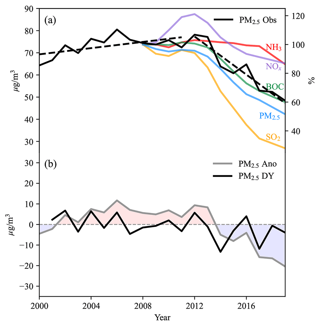
Figure 1 Variation in (a) winter PM_2.5 concentration (black; unit: µg m⁻³), (b) PM_2.5 anomalies (gray; compared to the mean of 2000–2019; unit: µg m⁻³) and PM_2.5 DY (black; unit: µg m⁻³). Color lines in (a) indicate relative variations in annual emissions (compared to that in 2008, unit: %) of ammonia (NH₃; red), nitrogen oxide (NO_x; purple), BOC (green), PM_2.5 (blue) and sulfur dioxide (SO₂; yellow) in the east of China. The black dashed line in (a) indicates the linear trend of PM_2.5 concentration.

2.2 Isolation of socioeconomic PM_2.5

We employed the simulated annual mean PM_2.5 concentrations that exclude the meteorological contributions to represent the impacts of anthropogenic emissions. Compared with the direct use of emission inventory of primary pollutants, the isolated socioeconomic PM_2.5 (SE-PM_2.5) involved both results of emission changes and follow-up physical and chemical reactions in the air. To remove the meteorological influences from the TAP PM_2.5 data, we used chemical transport models and emission inventories to separate the contributions from emission and meteorology changes. Following the approach proposed by Xiao et al. (2021), we used a “fixed-emission” scenario to quantify the impacts of interannual meteorological variation on PM_2.5 concentration in the Community Multiscale Air Quality (CMAQ) model. Subsequently, a full simulation with year-by-year emissions and meteorology was completed. Differences between the “fixed-emission” simulation and the full simulation were considered to be PM_2.5 concentrations driven by anthropogenic emissions. These data have been analyzed to quantify relative influences of different drivers on PM_2.5-related deaths in China (Geng et al., 2021b).

2.3 Year-to-year increment prediction

The year-to-year increment approach is proposed to improve the skill of climate prediction (Wang et al., 2008), in which the predicted object is not climate anomalies but is the difference between the current and the previous year (DY). After adding the predicted DY to the observed predictand in the year before, the final predicted results during 2001–2019 were obtained. Based on full use of observations in the previous year, the gradually changing trend and inter-decadal components can be reproduced well. The anthropogenic natural forcing predictand could be represented by Y = YS + YC, where YS and YC denote the slowly varying socioeconomic and climatic components, respectively. In the DY approach, which was expressed by

$$\begin{array}{rl}\text{DY}=& Y_t-Y_{t-\mathrm{1}}=\left({\text{YS}}_t+{\text{YC}}_t\right)-\left({\text{YS}}_{t-\mathrm{1}}+{\text{YC}}_{t-\mathrm{1}}\right)\\ =& \left({\text{YS}}_t-{\text{YS}}_{t-\mathrm{1}}\right)+\left({\text{YC}}_t-{\text{YC}}_{t-\mathrm{1}}\right),\end{array}$$

the subscripts t and t−1 indicate the current and the previous years. Before 2013, the difference between anthropogenic emissions in two adjacent years was small, and Yin and Wang (2016a) assumed $\left({\text{YS}}_t-{\text{YS}}_{t-\mathrm{1}}\right)\approx \mathrm{0}$ and proposed that DY was mainly influenced by climate variability. However, due to significant reduction of anthropogenic emissions after the implementation of China's Air Pollution Prevention and Control Action Plan (Zhang and Geng, 2020), the assumption of $\left({\text{YS}}_t-{\text{YS}}_{t-\mathrm{1}}\right)\approx \mathrm{0}$ was no longer completely valid. Therefore, it is meaningful to consider the information of rapid emission changes and re-build the prediction model (Yin et al., 2022).

1. Seasonal prediction model based on SE-PM_2.5(SP-SE). This prediction model unilaterally emphasized the impacts of human activities and was trained by DY of SE-PM_2.5 in each grid.

2. Seasonal prediction model based on preceding climate variability (SP-CV). This prediction model was highly focused on the impacts of climate condition and trained by DY of closely related climate factors.

3. Seasonal prediction model based on both SE-PM_2.5and climate (SP-EC). The contributions of emissions and climate factors are incorporated into one prediction model, i.e., combining the PM_2.5 DY from SP-SE and SP-CV.

In the leave-one-out cross validation, root-mean-square error (RMSE), relative bias and correlation coefficient (CC) were calculated. When discussing the CC after the detrending, the linear trend was removed by stages (i.e., winters of 2001–2011 and 2012–2019). The percentage of the same sign (PSS; same sign means the mathematical sign of the fitted and observed PM_2.5 anomalies was the same) was also computed.

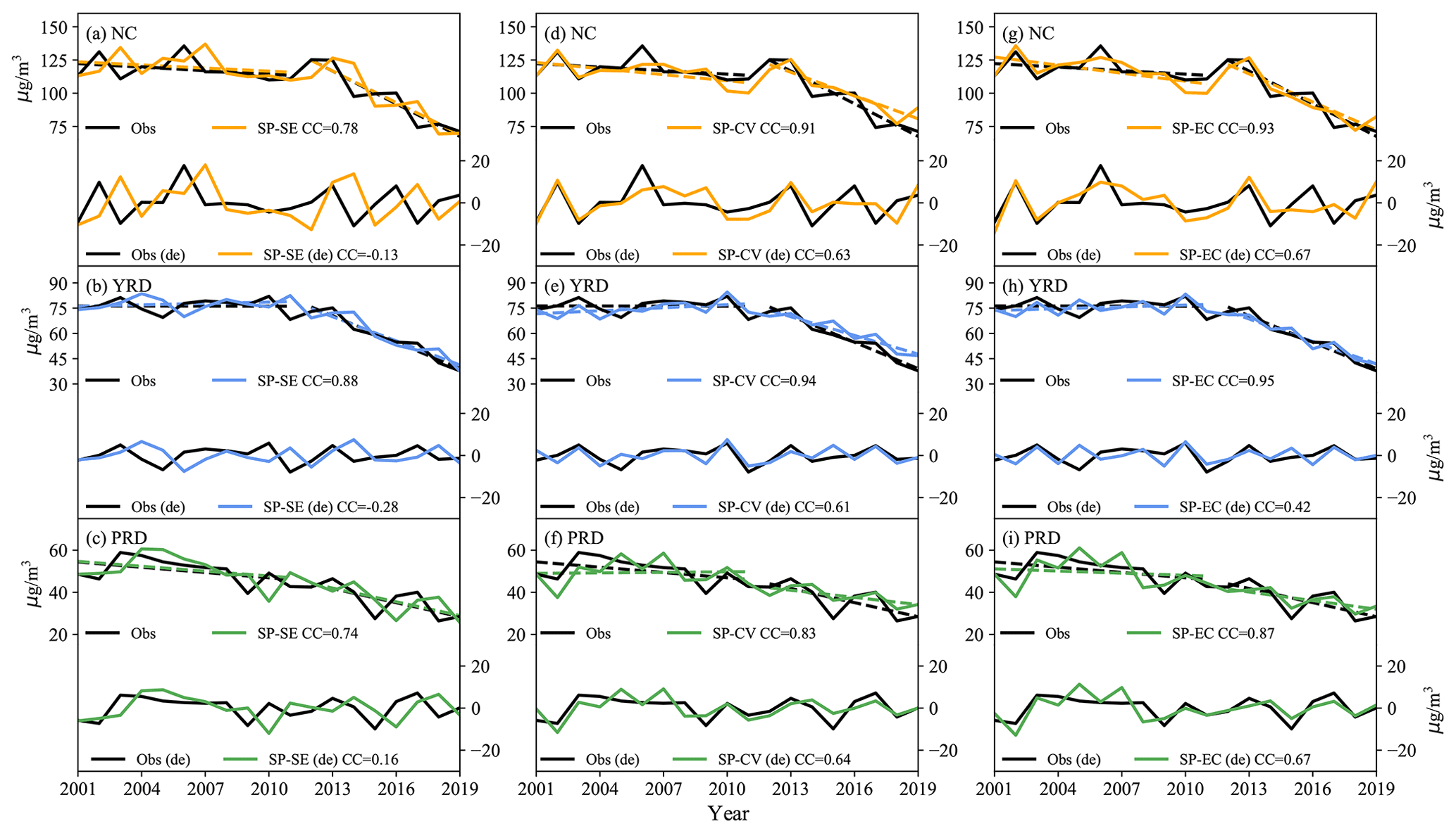
Figure 2 Variations in reanalysis (black) and SP-SE predicted winter PM_2.5 concentration in (a) NC (orange), (b) the YRD (blue), and (c) the PRD (green) from 2001 to 2019 before (upper) and after (lower) detrending. The predicted PM_2.5 is dependent on the leave-one-out validation. (d–f) are the same as (a–c) but for SP-CV. (g–i) are the same as (a–c) but for SP-EC.

3 Relative contributions of emission and climate predictors

3.1 Roles of emissions

Human activities are the major source of haze pollution in the east of China (Zhang and Geng, 2020), which implies that a large proportion of PM_2.5 concentration is predictable. Particularly, the large reduction of anthropogenic emissions since 2013 has determined the decreasing trend of winter PM_2.5 concentration (Fig. 1a). As mentioned above, the socioeconomic PM_2.5 (i.e., SE-PM_2.5) isolated by CMAQ could well reflect the impacts of human activities and was a potentially effective predictor for seasonal prediction of PM_2.5 concentration. As expected, the one-variable linear regression model based on anomalies of SE-PM_2.5 successfully reproduced different slopes of trend during 2001–2007, 2008–2013 and 2014–2019, but the predicted PM_2.5 concentration varied too smoothly (Fig. S1a in the Supplement). Furthermore, the quantities were underestimated when observed PM_2.5 concentration increased and overestimated when PM_2.5 concentration rapidly decreased. To eliminate the influence of trend shift, we calculated DY of PM_2.5 and SE-PM_2.5. Compared with its anomalies, PM_2.5 DY did not show a significant trend but displayed regularly oscillating characteristics (Fig. 1b), and its predictability was much better (Wang et al., 2008). The SP-SE model was trained by DY of SE-PM_2.5 in each grid to predict PM_2.5 DY. After adding the predicted PM_2.5 DY to observed PM_2.5 in the previous year, the final PM_2.5 concentration was obtained. The CC between predicted and observed PM_2.5 was 0.87 during 2001–2019 in the east of China. The underestimated (2001–2007) and overestimated (2014–2019) values in Fig. S1a were largely corrected, and interannual variation also appeared in the results of SP-SE prediction (Fig. S1b). The staged trends from the SP-SE model almost overlapped with the observed trends, indicating the model performed well in capturing the changes in trend (Fig. S2).

Figure 3 Spatial patterns (a–d) and corresponding PCs (e–h) of the first four EOF modes for winter PM_2.5 DY in the east of China during 2000–2019. The variance accounted for by each EOF mode is given in the panel.

Table 1 The leave-one-out validated root-mean-square errors (RMSEs), relative biases (absolute bias mean; %) and percentages of same sign (PSS) for three statistical models.

North China (NC; 34–42^∘ N, 114–120^∘ E), the Yangtze River Delta (YRD; 27–34^∘ N, 117–122^∘ E) and the Pearl River Delta (PRD; 21.5–25^∘ N, 112–116^∘ E) are three regions that have been experiencing severe PM_2.5 pollution (Yin et al., 2015). Thus, the performance of the SP-SE model in NC, the YRD and the PRD was validated separately (Table 1, Fig. 2a–c). The RMSEs were 12.2, 6.2 and 6.8 µg m⁻³in NC, the YRD and the PRD, respectively (Table 1). Larger RMSE in NC did not indicate the SP-SE model performs worse in NC than in the YRD and the PRD because the mean value of PM_2.5 concentration was the highest in NC. The relative bias (absolute bias$/$mean) in NC was 8.5 %, which was smaller than that in the PRD (12.9 %). Consistent with its performance in the east of China, the SP-SE model also reproduced well the staged trends in NC, the YRD and the PRD (Fig. 2a–c). However, when the linear trend was removed, the CC between predicted and observed PM_2.5 significantly decreases in all the three PM_2.5-polluted regions (NC: from 0.78 to −0.13; YRD: from 0.88 to −0.28; PRD: from 0.74 to 0.16). That is, the prediction model trained by the socioeconomic PM_2.5 could predict the values and staged linear trends well. However, it certainly had no ability to simulate the interannual variability in PM_2.5 concentration.

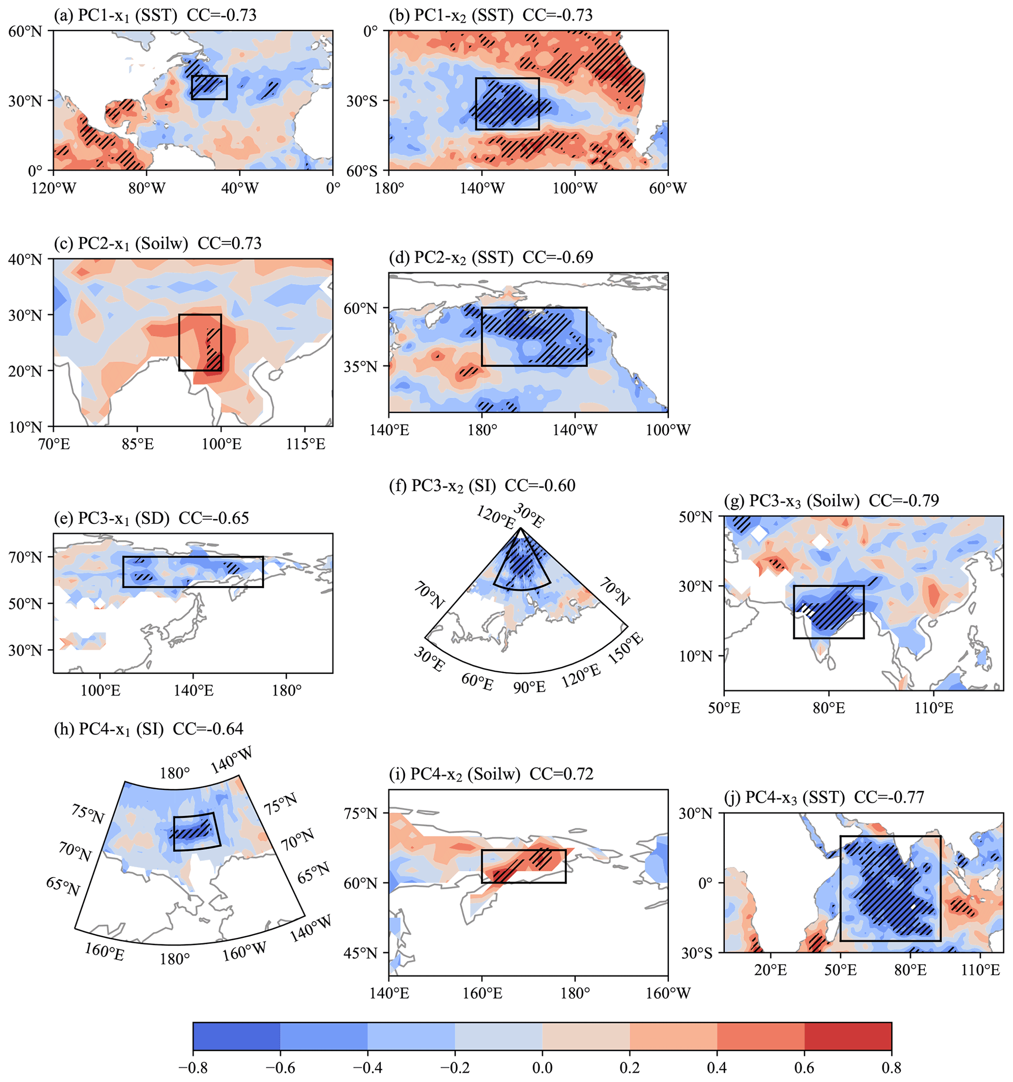
Figure 4 CCs between climate predictors and (a–b) PC1, (c–d) PC2, (e–g) PC3, (h–j) PC4 from 2000 to 2019. The predictors for PC1 are (a) September SST over the South Pacific Ocean and (b) October SST over the Sargasso Sea. The predictors for PC2 are (c) October Soilw over the Indo-China Peninsula and (d) June–August SST over the Gulf of Alaska. The predictors for PC3 are (e) October SD over eastern Siberia, (f) October SI over the Kara Sea and (g) September–October Soilw over the Indian Peninsula. The predictors for PC4 are (h) October SI over the Chukchi Sea, (i) October Soilw over the Kamchatka Peninsula and (j) August–September SST over the Arabian Sea and the Bay of Bengal. The slashes indicate CCs exceeding the 95 % confidence level. The black boxes indicate the regions over which the predictors are calculated.

3.2 Impacts of climate variability

Decomposition and prediction of dominant modes of climate conditions were applied in short-term prediction of precipitation (Huang et al., 2022) and surface air temperature (Hsu et al., 2020) in the east of China. In this study, we decompose the first four leading modes of PM_2.5 DY during 2001–2019 (accumulated variance contribution = 81 %) produced by empirical orthogonal function (EOF) analysis, built a prediction model for each respective principal component, recalculated the predicted PM_2.5 DY by projecting the predicted PCs onto the observed EOF spatial patterns and finally added the predicted PM_2.5 DY to the observation in the previous year to finish the development of SP-CV (Fig. S3, Table S1 in the Supplement). The interannual–decadal variation in haze pollution could be explained well by meteorological condition and preceding climate forcings (Yin et al., 2020) such as the Arctic sea ice extent (Wang et al., 2015; Yin et al., 2019), Eurasia snow (Zou et al., 2017) and soil moisture (Yin and Wang, 2018), and SST in the Pacific (Yin and Wang, 2016b; He et al., 2019) and Atlantic (Yin and Zhang, 2020). Prediction signals from these climate anomalies could be observed before winter and had specific physical implications.

Figure 5 Scatter plots of normalized observed (x axis) and predicted (y axis) PC1 (blue), PC2 (orange), PC3 (green) and PC4 (gray) from 2000 to 2019. The predicted PCs are dependent on the leave-one-out cross validation.

The first EOF mode of PM_2.5 DY illustrated the heavily haze-polluted status in NC (Fig. 3a, e). According to the correlation analysis, the September SST DY in the southwest Pacific (CC with PC1 = −0.73; Fig. 4a) and October SST DY in the Sargasso Sea (CC = −0.73; Fig. 4b) were selected to be the two predictors for PC1 of PM_2.5 DY (Table S1). Both of the predictors had close relationships with the dipole pattern of Eurasian cyclonic and northeast Asian anti-cyclonic circulations (Fig. S4b, c), which were identical to those associated with PC1 (Fig. S4a) and could restrain the invasion of cold air from high latitude into NC. The second EOF mode of PM_2.5 DY showed a “north–south” dipole pattern (Fig. 3b, f). The variations in PM_2.5 DY in Huanghuai and the YRD accounted for a large proportion. The October soil moisture DY in the Indo-China Peninsula (CC with PC2 = 0.73; Fig. 4c) and June–August SST DY in the Gulf of Alaska (CC = −0.69; Fig. 4d) were selected to build the prediction model of PC2 (Table S1). The anomalous atmospheric circulation associated with PC2 and its predictors could enhance cold air invasion to NC (strong northerlies) but prevented the cold air from moving further south (weak 10 m winds in Fig. S4d–f).

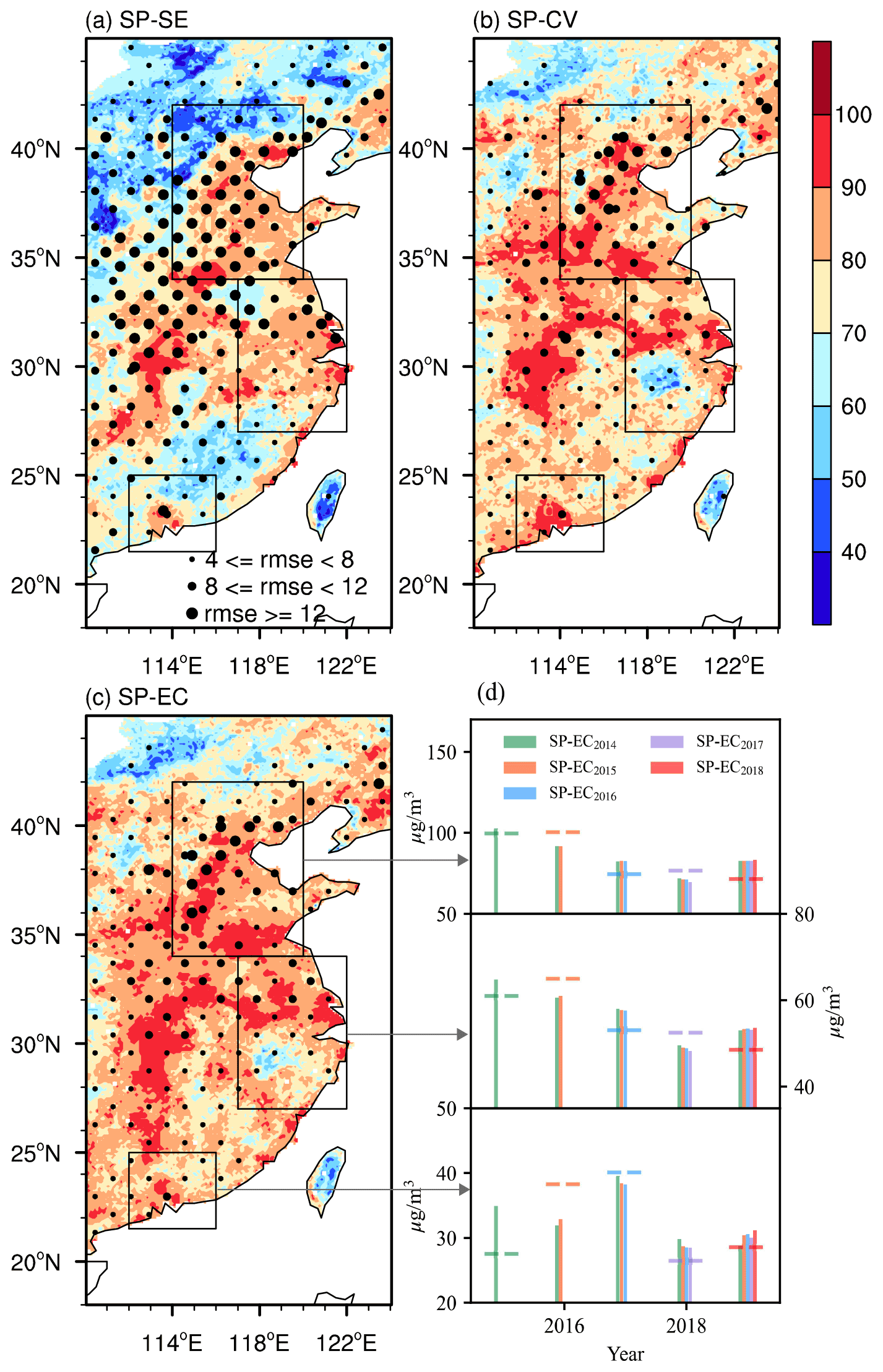
Figure 6 Distributions of PSS (shadings) and RMSE (dots) from (a) SP-SE, (b) SP-CV and (c) SP-EC. The boxes represent NC, the YRD and the PRD, respectively, and the arrows point to the SP-EC-predicted PM_2.5 in recycling independent tests (bars) and observations (dashed lines) corresponding to the area. The subscript in the legend of (d) indicates the model trained from 2000 to this year, and the PM_2.5 from the next year to 2019 are independently predicted.

The third EOF mode indicated a triple pattern with centers located in the east of Inner Mongolia, the Fenwei Plain and South China (Fig. 3c, g). The Fenwei Plain was highly polluted and gained great attention in recent years, while the other two centers have relatively better air quality (Zhao et al., 2021). The October snow depth DY in eastern Siberia (CC with PC3 = −0.65; Fig. 4e), October sea ice DY in the north to Barents Sea (CC = −0.60; Fig. 4f) and September–October soil moisture DY in the Indian Peninsula (CC = −0.79; Fig. 4g) were considered in the prediction model (Table S1). The predictors possibly induced atmospheric responses in winter (Fig. S4h–j) that were similar to PC3 (Fig. S4g). The abnormal northerlies over North China and South China enhanced the horizontal dispersion of haze particles (Zhong et al., 2019), while the weak wind speed and surface wind convergence in central China were conductive to the accumulation of pollutants. A statistical model (Table S1) was also developed to predict the “east–west” dipole shown in the fourth EOF mode (Fig. 3d,h) based on October sea ice DY in the Chukchi Sea (CC = −0.64; Fig. 4h), October soil moisture DY on the Kamchatka Peninsula (CC = 0.72; Fig. 4i) and August–September SST DY in the Arabian Sea (CC = −0.77; Fig. 4j). The atmospheric anomalies in the lower troposphere and near surface, which were associated with the above predictors and PC4, also had similar impacts on haze pollution (Fig. S4k–n).

As shown in Fig. 5, multiple linear regression models demonstrated good performance in simulating the variation in each PC. The CCs between observed and predicted first to fourth PCs were 0.82, 0.80, 0.75 and 0.93, respectively, all of which were above the 99 % confidence level, indicating that the model successfully reproduced each individual EOF mode. Meanwhile, the yearly increment approach had the ability to address the trend and its changes that were not obviously mutational (Yin and Wang, 2016a). The CC between observed and predicted PM_2.5 concentrations before (after) detrending by stages was 0.91 (0.63) in NC, 0.94 (0.61) in the YRD and 0.83 (0.64) in the PRD in the leave-one-out validation (Fig. 2d–f). Thus, the SP-CV model simulated well both the trend of and the interannual variation in PM_2.5 concentration in the east of China. In addition, the RMSEs in NC, the YRD and the PRD were 8.0, 4.8 and 5.2 µg m⁻³, and the relative biases were 5.3 %, 6.2 % and 9.9 %, respectively (Table 1), all of which were obviously smaller than those of SP-SE. The PSS, which is an important indicator of climate prediction, was also evaluated relative to the winters of 2001–2019. The area-averaged PSS from SP-CV was 79.9 % in the east of China, which was 7.9 % higher than that from SP-SE (Fig. 6). Although the SP-CV model performed better than the SP-SE, especially that it could capture the sharp downward trend after 2013 in NC and YRD, the RMSEs of the SP-CV simulations for the period 2015–2019 increased up to 11.6, 6.5 and 5.3 µg m⁻³in NC, the YRD and the PRD compared to that of the SP-SE simulations. Obvious positive biases were found in the predictions of PM_2.5 concentration after 2014 (Fig. 2d–f) because the SP-CV model was short of information about the super-strict emission regulations (Fig. S2). Based on different levels of haze pollution, various degrees of air pollution control were carried out in NC, the YRD and the PRD (Zhang and Geng, 2020). In NC, where anthropogenic emissions were most prominently restricted, the predicted biases were also the largest (Fig. 2d). The predicted biases were the smallest in the PRD, while those in the YRD were in between. These results were consistent with different intensities of pollution control in the three regions (Fig. 2e, f), which further indicated the importance of fully taking into account the impacts of climate variability and anthropogenic emissions.

Figure 7 Scatter plots of the reanalysis (x axis) and predictions of (y axis) PM_2.5 concentration by SP-CV (green) and SP-EC (blue) in (a) the east of China, (b) NC, (c) the YRD and (d) the PRD. The points during 2012–2019 are filled and the short lines between SP-CV and SP-EC points indicate the calibrations.

4 PM_2.5 prediction with integrated factors

As mentioned above, the SP-SE model trained by the SE-PM_2.5 DY considered the impacts of emission changes one-sidedly and could simulate well the values and staged trends. However, it completely failed to reproduce the interannual variation in winter PM_2.5 concentration in the east of China (Fig. 2a–c). Differently, the predictors of climate variability could introduce the interannual variation in winter PM_2.5, and the yearly increment approach had the ability to bring in the slow trend. The SP-CV model successfully predicted most of the trend of and interannual variation in PM_2.5 concentration (Fig. 2d–f) but underestimated the sharp decreasing trend (Fig. S2), which led to positive forecast biases after 2013 (Fig. 2d–f).

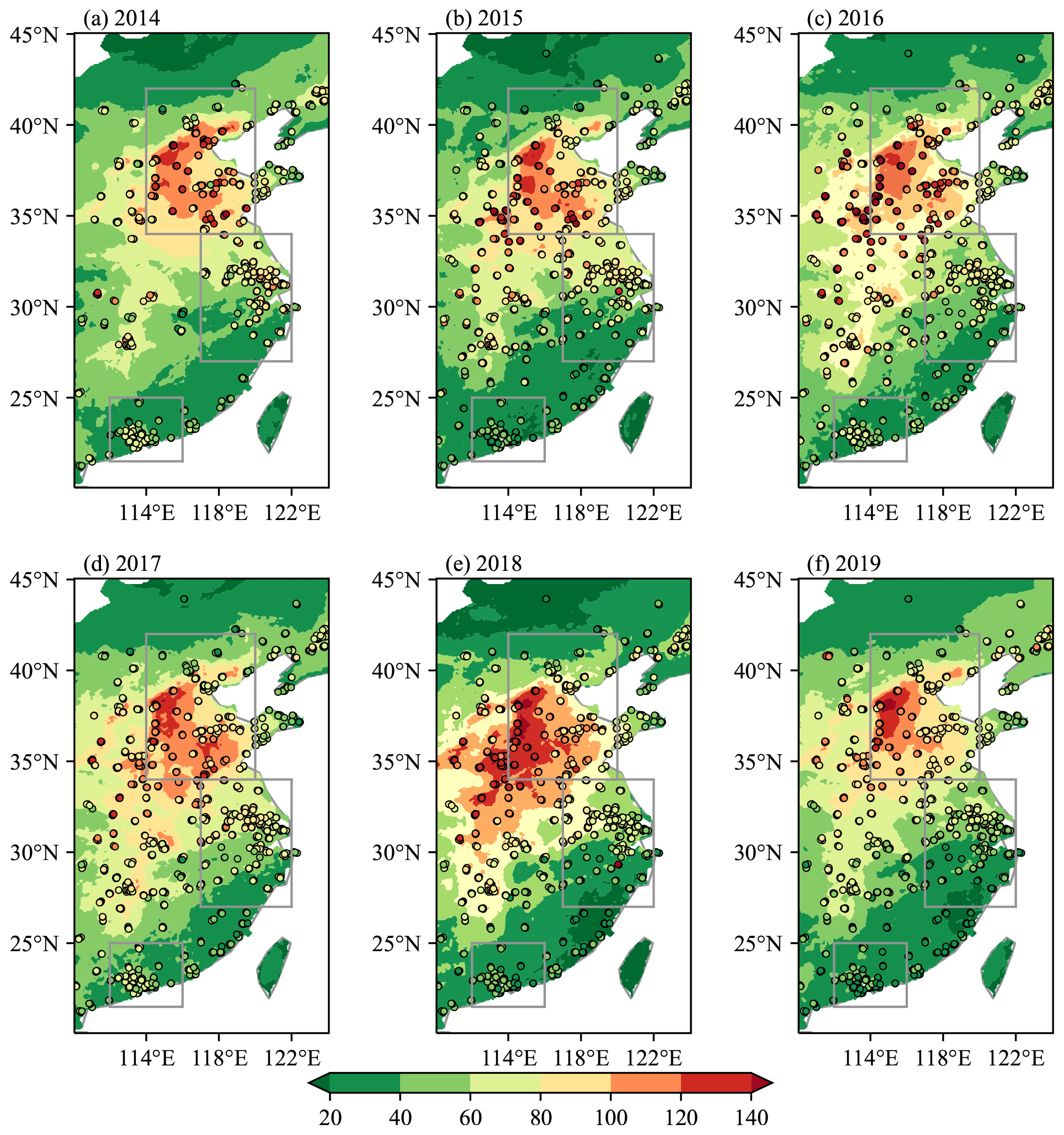
Figure 8 SP-EC-predicted (shading) and site-observed (scatter) PM_2.5 concentrations (units: µg m⁻³) in (a) 2014, (b) 2015, (c) 2016, (d) 2017, (e) 2018 and (f) 2019. The boxes represent NC, the YRD and the PRD respectively.

To fully contain predictive signals of human activities and climate anomalies, the predicted PM_2.5 DY values from SP-SE and SP-CV model for the current year were added up, and the sum was added to PM_2.5 observations in the previous year to develop the final prediction model, i.e., the SP-EC model. As expected, the performance of SP-EC model was better than that of both SP-SE and SP-CV models. Area-averaged PSS was 81.4 % in the east of China (Fig. 6). The CC between observed and SP-EC-predicted PM_2.5 concentrations before (after) detrending was 0.96 (0.74) in the east of China; the RMSE was 2.7 µg m⁻³, which was 43.8 % (32.5 %) smaller than the RMSE of SP-SE (SP-CV) in the leave-one-out validation. That is, the trend simulated by the SP-EC model almost overlapped with the trend of observations (similar to results of SP-SE), and the interannual variation was also reproduced (similar to results of SP-CV). The CCs between observed and SP-EC-predicted PM_2.5 concentrations before (after) detrending were 0.93 (0.67) in NC, 0.95 (0.42) in the YRD and 0.87 (0.67) in the PRD (Fig. 2g–i). The RMSEs were 6.8 in NC, 4.2 in YRD and 4.7 µg m⁻³ in PRD, which were 44.3 % (15.0 %), 32.3 % (12.5 %) and 30.9 % (9.6 %) lower than that of SP-SE (SP-CV), indicating greater improvements in NC than in the other two regions (Table 1). According to the relative biases, the SP-EC model also demonstrated a better skill in NC (5.1 %) than that in the YRD (4.9 %) and the PRD (8.8 %) in the leave-one-out validation. As shown in Fig. 7, the decreases in PM_2.5 resulting from the implementation of strict emission control measures in recent years were also reproduced by the SP-EC model. The evident and positive biases in the SP-CV results were largely corrected in the east of China, NC, the YRD and the PRD (Fig. 7).

High spatial resolution was one of the advantages of the seasonal prediction model developed in this study. That is, the SP-EC model could predict winter PM_2.5 concentration at each 10 km × 10 km grid in the east of China. When only considering emission predictors (i.e., SP-SE), RMSEs>12 µg m⁻³ were found in the middle part of the study region, and the PSS was lower than 60 % in South China and Inner Mongolia (Fig. 6a). When only considering climate predictors (i.e., SP-CV), RMSEs>12 µg m⁻³ existed in Beijing and its surrounding areas, and PSS significantly increased compared to the result of SP-SE (Fig. 6b). When integrating both of the emission predictors and climate predictors (i.e., SP-EC), the RMSE in each grid further decreased, and the PSS also increased (Fig. 6c). In the middle part of the study region, the PSS was higher than 80 %. In view of gaps between site observations and model simulations, the SP-EC-predicted PM_2.5 concentrations were compared with site observations (Fig. 8). NC was the most severely polluted area, and the SP-EC model could capture the PM_2.5 values and interannual differences. Particularly, the SP-EC model reproduced the sudden rebound of PM_2.5 pollution in 2018 (Fig. 8e) that was mainly the result of climate anomalies (Yin and Zhang, 2020).

Due to the limitation of the short sequence of data, recycling independent tests (RITs) were designed to further verify the performance of the SP-EC model. In the RIT predictions, the prediction model was trained by samples from 2001 to the expiration year of training data, and the PM_2.5 anomalies from the next year to 2019 were independently predicted. For example, the prediction model trained by the data from 2001 to 2014 can produce independent predictions from 2015 to 2019. The expiration year of the training data moved forward from 2015 to 2019, so there were 15 independent predictions. The PM_2.5 concentration was independently predicted five times for 2019, four times for 2018, and so on. The PSS of PM_2.5 anomalies was 100 %, not only relative to winters of 2001–2019 but also 2015–2019, indicating a high accuracy of prediction in the east of China. The predicted values for each year did not vary much (Fig. 6d), indicating a high reliability and robustness of the model. For example, when the SP-EC model was trained by the samples only from 2000 to 2014, the predicted PM_2.5 anomalies for 2018 and 2019 were also close to the results of leave-one-out validations and the measurements.

5 Conclusions and discussion

The change in haze pollution consisted of long-term trends, interannual–decadal variations, synoptic disturbances and so on. Seasonal prediction focused on predicting long-term trends and interannual–decadal variations 1–3 months in advance (Wang et al., 2021). Because of the limitation of short observational period, many previous studies employed the number of haze days as a proxy of PM_2.5 pollution to build statistical prediction models (Yin and Wang, 2016a; Yin et al., 2017; Dong et al., 2021; Zhao et al., 2021; Chang et al., 2021). Since 2020, several high-resolution PM_2.5 reanalysis datasets have been successively released, which greatly increased the possibility for direct seasonal prediction of PM_2.5 concentration that is more familiar to decision makers and the public (Yin et al., 2021).

In this study, two seasonal prediction models were separately trained by emission factor (i.e., SP-SE) or preceding climate predictors (i.e., SP-CV) to discuss their relative contributions. The SP-SE model could simulate the slow rising trend of PM_2.5 concentration before 2012 and the strong downward trend after 2012. However, it was incapable of importing the interannual component. The SP-CV model benefited from the year-to-year increment approach and could introduce a large portion of the linear trend except the sharp decrease in winter PM_2.5 concentration from 2013. Furthermore, the SP-CV model performed well in predicting the obvious interannual variation in PM_2.5 concentration. We integrated the emission and climate factors to establish the final prediction model (i.e., SP-EC), which could reproduce well both the trend of and the interannual variation in PM_2.5 concentration. The area-averaged PSS was 81.4 % in the east of China and CC between observed and predicted PM_2.5 concentrations before (after) the detrending was 0.96 (0.74). The RMSEs were 6.8 in NC, 4.2 in the YRD and 4.7 µg m⁻³in the PRD, which were 44.3 % (15.0 %), 32.3 % (12.5 %) and 30.9 % (9.6 %) lower than the results of SP-SE (SP-CV). Due to the implementation of the super-strict emission control measures, the air quality has been substantially improved, and this improvement was also perfectly predicted by the SP-EC model. During recycling independent tests, the PSS of PM_2.5 anomalies was 100 %, demonstrating high accuracy and robustness. The high-resolution PM_2.5 prediction could provide scientific support for air pollution control at the regional and city levels. For example, real-time PM_2.5 prediction is highly demanded for determining how to reduce anthropogenic emissions and how much should be reduced; 10 km × 10 km gridded PM_2.5 information also had the potential to support finely and dynamically regional management and collaborations.

This study mainly focused on developments of a seasonal PM_2.5 prediction model. Related theories and methods are still exploratory and need further discoveries. Although the SP-EC model was proven to be skilled, the underlying physical mechanisms of climate predictors were not sufficiently explained and needed further in-deep studies. As shown in Fig. 8f, the SP-EC model failed to predict well the evident PM_2.5 drops in the east of China caused by COVID-19 quarantines in the winter of 2019 (especially February in 2020) (Yin et al., 2021). Therefore, such sudden fluctuations of PM_2.5 concentration were not involved in the established prediction model. Furthermore, the EOF pattern of PM_2.5 possibly changed under climate change and must influence the climate component of PM_2.5, which should be updated in time. Although the SP-EC model had high spatial resolution, it could only output winter mean PM_2.5 concentration. It was meaningful to build sub-seasonal models to provide more detailed predictions. Modern weather and climate forecasts were heavily dependent on numerical prediction models. Thus, it is imperative to design and develop numerical models that target routine seasonal prediction of air pollution (Yin et al., 2021).