Bayesian assessment of chlorofluorocarbon (CFC), hydrochlorofluorocarbon (HCFC) and halon banks suggest large reservoirs still present in old equipment

Halocarbons contained in equipment such as air conditioners, fire extinguishers, and foams continue to be emitted after production has ceased. These “banks” within equipment and applications are thus potential sources of future emissions, and must be carefully accounted for in order to differentiate nascent and potentially illegal production from legal banked emissions. Here, we build on a probabilistic Bayesian model, previously developed to quantify chlorofluorocarbon (CFC-11, CFC-12, and CFC-113) banks and their emissions. We extend this model to a suite of banked chemicals regulated under the Montreal Protocol (hydrochlorofluorocarbon, HCFC-22, HCFC-141b, and HCFC-142b, halon 1211 and halon 1301, and CFC-114 and CFC-115) along with CFC-11, CFC-12, and CFC-113 in order to quantify a fuller range of ozone-depleting substance (ODS) banks by chemical and equipment type. We show that if atmospheric lifetime and prior assumptions are accurate, banks are most likely larger than previous international assessments suggest, and that total production has probably been higher than reported. We identify that banks of greatest climate-relevance, as determined by global warming potential weighting, are largely concentrated in CFC-11 foams and CFC-12 and HCFC-22 non-hermetic refrigeration. Halons, CFC-11, and CFC-12 banks dominate the banks weighted by ozone depletion potential (ODP). Thus, we identify and quantify the uncertainties in substantial banks whose future emissions will contribute to future global warming and delay ozone-hole recovery if left unrecovered.

1 Introduction

The Montreal Protocol regulates the production of ozone-depleting substances (ODS), and its implementation has avoided a world with catastrophic stratospheric ozone depletion (Newman et al., 2009). Globally, there has been a near-cessation of chlorofluorocarbon (CFC) and halon production since 2010, and global production of the replacement hydrochlorofluorocarbons (HCFCs) is scheduled to be phased out by 2030. Despite production phase-out, these chemicals persist in old equipment produced prior to phase-out, such as refrigeration, air conditioners, foams, and fire extinguishers. These reservoirs of materials (termed “banks”) continue to be sources of emissions (e.g., Carpenter et al., 2018). Previously published estimates of bank sizes and bank emissions vary widely due to different estimation techniques that incorporate incomplete or imprecise information (Kuijpers and Verdonik, 2009; Montzka et al., 2003). This uncertainty obscures the ongoing attribution of emissions and undermines international efforts to evaluate global compliance with the Montreal Protocol. In earlier work, Lickley et al. (2020, 2021) developed a Bayesian probabilistic banks model for CFCs that incorporates the widest range of constraints to date (Lickley et al., 2020, 2021). Here, we extend this model to the suite of major chemicals regulated by the Montreal Protocol that are subject to banking.

Previously published assessments typically rely on one of three modeling approaches to estimate bank sizes and then estimate emissions associated with these banks. In the “top-down” approach (e.g., Montzka et al., 2003), banks are estimated as the cumulative difference between reported production and observationally derived emissions. However, by taking the cumulative sum of a small difference between two large values, small biases in emissions or reported production estimates can propagate into large biases in bank estimates (Velders and Daniel, 2014). Some type of bias is thus expected since total production has very likely been greater than reported production due to both the under-reporting of production (e.g., Gamlen et al., 1986; Montzka et al., 2018) and the exclusion of point-of-production losses in reported production values. Further estimates of emissions rely on observed concentrations along with global lifetime estimates, which have large uncertainties associated with them (Ko et al., 2013).

The second approach relies on a “bottom-up” accounting method (Ashford et al., 2004; Campbell et al., 2005) where the inventory of sales by equipment type are carefully tallied along with estimated release rates by application use. The bottom-up approach also relies on sales data from surveys of various equipment types and products as well as estimates of their respective leakage rates (Campbell et al., 2005). These are all subject to uncertainties, which contribute to uncertainties in bottom-up bank estimates as well. A limitation of the bottom-up accounting method is that observed atmospheric concentrations are used only as a qualitative check and are not explicitly accounted for in the analysis. Another important limitation is that data used in this method are unobserved and rather rely on estimated processes along with reported data, such as production or sales of equipment. Thus any bias in reporting could propagate into large biases in bank estimates.

The third approach, and the one used in more recent ozone assessments such as the World Meteorological Organization (WMO, 2011, 2018, 2014), uses a hybrid approach to calculate banks. Bottom-up banks estimated for 2008 are used as a starting point for the calculations. These banks are taken from Campbell et al. (2005) and represent interpolated values from the 2002 and 2015 estimates. The banks are then brought forward to the present time by adding the cumulate reported production and subtracting the cumulative observationally derived emission from 2008 through the present. This approach is consistent with 2008 bottom-up bank estimates by design, however, as time between 2008 and the present has grown, the cumulative errors associated with the top-down approach become larger.

The modeling approach applied in the present study relies on Bayesian inference of banks (Lickley et al., 2020, 2021) where banks are estimated using an approach called Bayesian Parameter Estimation (BPE). In this approach, a simulation model of the bottom-up method is developed, where prior distributions of input parameters are constructed from previously published values, accounting for large uncertainties in production and bank release rates. The simulation model simultaneously models banks, emissions, and atmospheric concentrations. Parameters in the simulation model are then conditioned (or updated) on observed concentrations by applying Bayes' rule. The final result is a posterior distribution of banks by chemical and equipment type, along with an updated estimate of production and release rates for each equipment type. This approach incorporates data and assumptions from both the bottom-up and top-down approaches, providing a simulation model consistent with the bottom-up accounting method while also being consistent with observed concentrations within their uncertainties.

The remainder of the paper includes the following: Sect. 2 presents the Bayesian modeling approach along with data used in the analysis. Section 3 provides a summary of the results of our analysis for each of the chemicals considered here. Finally, Sect. 4 provides a discussion of our primary findings and limitations of the analysis.

2 Methods

The Bayesian modeling approach from Lickley et al. (2020, 2021) draws on a Bayesian analysis approach called Bayesian melding, designed by Poole and Raftery (2000), that allows us to apply inference to a deterministic simulation model. We employ a version of this method that we henceforth refer to as the Bayesian Parameter Estimation (BPE), which allows for input parameter uncertainty (Hong et al., 2005; Bates et al., 2003). The model flow is implemented as follows: first we develop a deterministic simulation model, representing the “bottom-up” accounting method that simultaneously simulates banks, emissions, and mole fractions for each chemical and equipment type. In this analysis, the chemicals considered include CFC-11, CFC-12, CFC-113, CFC-114, CFC-115, HCFC-22, HCFC-141b, HCFC-142b, halon 1201, and halon 1311. Prior distributions for each of the input parameters are based on previously published estimates. We then specify the likelihood function as a function of the difference between observed and simulated mole fractions. Finally, we estimate posterior distributions of both the input and output parameters by implementing Bayes' Rule using a sampling procedure. Each of the steps of the BPE are described in more detail below.

2.1 Simulation model

The simulation model, comprised of Eqs. (1)–(5), simultaneously models banks, emissions, and mole fractions for each chemical by equipment type for all years with available data up until 2019. Starting dates differ by chemical, see “Details on Simulation Model” in the Supplement tables. The simulation model is specified as follows:

$$\begin{array}{}\text{(1)}& B_{j,t+\mathrm{1}}=\left(\mathrm{1}-{\mathrm{RF}}_{j,t}\right)\times B_{j,t}+(\mathrm{1}-{\mathrm{DE}}_{j,t})\times P_{j,t},\end{array}$$

where B_j, t, is banks and P_j, t is production of equipment category j in year t. The fraction of the released bank is reflected by RF_j, t and DE_j, t reflects the fraction of production that is directly emitted in equipment category j in year t. These same parameters are used to simulate emissions, $E_{j,t}:$

$$\begin{array}{}\text{(2)}& E_{j,t+\mathrm{1}}={\mathrm{RF}}_{j,t}\times B_{j,t}+{\mathrm{DE}}_{j,t}\times P_{j,t}.\end{array}$$

Total banks, B_Total, t, and total emissions, E_Total, t, are then estimated as the sum across all N equipment categories:

$$\begin{array}{}\text{(3)}& {\displaystyle }{B}_{\mathrm{Total},t}={\sum }_{j=\mathrm{1}}^N{B}_{j,t},\text{(4)}& {\displaystyle }{E}_{\mathrm{Total},t}={\sum }_{j=\mathrm{1}}^N{E}_{j,t}.\end{array}$$

For chemicals where feedstock usage is reported, an additional term in Eq. (4) is included that accounts for feedstock emissions. Emissions, along with an assumed atmospheric lifetime, τ_t, taken as the Ko et al. (2013) multimodel time-varying mean, are then used to simulate atmospheric mole fractions, MF_t:

$$\begin{array}{}\text{(5)}& {\mathrm{MF}}_{t+\mathrm{1}}=\exp \left({\displaystyle \frac{-\mathrm{1}}{{\mathit{\tau }}_t}}\right)\times {\mathrm{MF}}_t+A\times E_{\mathrm{Total},t},\end{array}$$

where A is a constant that converts units of emissions by mass to units of mole fractions, and also takes into account a fixed factor of 1.07 taken from Daniel et al. (2007) that accounts for the discrepancy between surface mole fraction concentrations and the global mean value.

2.2 Prior distributions

The input parameters in the simulation model described above require initial values to be assigned, along with their probability distributions. These prior distributions (“priors”) are developed to estimate mole fractions, emissions, and banks for CFC-11, CFC-12, CFC-113, CFC-114, CFC-115, HCFC-22, HCFC-141b, HCFC-142b, halon 1201, and halon 1311. Categories of bank equipment are defined by the categorization provided by the Alternative Fluorocarbons Environmental Acceptability Study (AFEAS 2001) which varies by compound (shown in Table 1). For halons, there is a single category of bank (fire extinguishing agent).

Table 1 Application type of halocarbon banks by chemical.

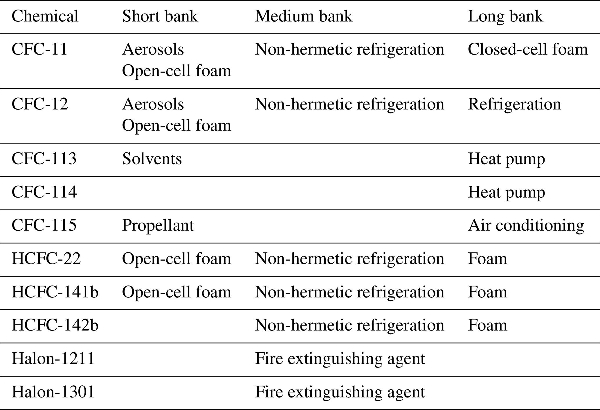
The AFEAS data report global annual production up to 2001, categorized by equipment type, which is generally grouped as short, medium and long banks. We use AFEAS data and categorization to develop our production priors and adopt the WMO (2003) correction where AFEAS production values are used up until 1989 and then scaled to match the United Nations Environmental Programme's (UNEP) global production values for all years following 1989. After AFEAS data ends, we assume that the relative production in each category remains constant for all years following 2001. Uncertainty in production priors is assumed to follow a multivariate log-normal distribution, where temporal correlation in production reporting bias is estimated in the BPE. Priors differ by chemical and are developed to be wide enough for atmospheric mole fraction priors to contain observations. See the Supplement for details on production priors for each chemical.

The emissions function by bank equipment type can be characterized by the fraction of production that is directly emitted during the year of production (DE) and the fraction of the bank that is emitted in each subsequent year. Prior estimates for the emissions function come from previously reported data and differ by chemical and equipment type (see the Supplement). Broadly speaking, it has been estimated that chemicals contained in short banks are fully emitted within the first 2 years after production, medium banks lose about 10 %–20 % of their material each year, and long banks can lose as little as 2 % of their material each year (Ashford et al., 2004). We use previously published estimates to develop emissions function priors specific to each chemical and bank type along with wide uncertainties, as specified in the Supplement.

Amounts of halocarbons used for feedstock production are available annually (UNEP/TEAP, 2021). A prior mean leakage rate of 2 % was assumed during production, which reflects an approximate average of values across different facilities (MCTOC, 2019).

2.3 Likelihood function

For each chemical, the likelihood function is a multivariate normal likelihood function of the difference between modeled and observed mole fractions:

$$\begin{array}{}\text{(6)}& P\left(D_{t\mathrm{1}},\mathrm{\dots }{D}_{tM}|\mathit{\theta }\right)={\displaystyle \frac{\mathrm{1}}{{\left(\mathrm{2}\mathit{\pi }\right)}^{\frac{M}{\mathrm{2}}}\sqrt{\left|\mathbf{S}\right|}}}\exp \left\{-{\displaystyle \frac{\mathrm{1}}{\mathrm{2}}}{\mathrm{\Delta }}^T{\mathbf{S}}^{-\mathrm{1}}\mathrm{\Delta }\right\},\end{array}$$

where D_t1,…D_tM is yearly globally averaged observed mole fractions for all years where observations are available and θ represents that vector of input and output parameters from the simulation model. The Δ denotes an M×1 vector of the difference between yearly observed and modeled mole fractions and is assumed to have a mean zero, and covariance function S​​​​​​​. Therefore, S represents the sum of uncertainties between observed and modeled mole fractions. While there are published estimates of uncertainties in observed mole fractions, we do not know the uncertainties in modeled mole fractions. We therefore estimate S separately for each chemical, as is done in Lickley et al. (2020). The off-diagonals in the covariance function incorporate a correlation term, ρ_S, which accounts for our assumption that there is high autocorrelation in the bias between modeled and observed mole fractions. Correlation terms for each chemical are reported in the Supplement along with prior estimates of the uncertainty parameters used for diagonal elements in S. Each column and row in S is therefore populated as

$${\mathbf{S}}_{i,j}={\mathit{\sigma }}_i{\mathit{\sigma }}_j{\mathit{\rho }}_{\mathrm{S}}^{|i-j|},$$

where σ_i and σ_j represent the sum of the uncertainties in observed and modeled mole fractions at time i and j, respectively, and are inferred in the BPE, whereas ρ_S is prescribed.

Observations come from the Advanced Global Atmospheric Gas Experiment (AGAGE; https://agage.mit.edu, last access: 29 March 2022) data set (Prinn et al., 2000, 2018), with the exception of CFC-11 and CFC-12 which, following Lickley et al. (2021), come from the AGAGE and the National Oceanographic and Atmospheric Administration's (NOAA) merged data sets (Engel et al., 2019). Data are aggregated into annual global mean mole fractions. The time frame of availability of observations differs by chemical (see the Supplement).

2.4 Posterior distributions

Following Bayes' Rule, we specify our posterior distribution as

$$\begin{array}{}\text{(7)}& P\left(\mathit{\theta }|D_{t\mathrm{1}},\mathrm{\dots },D_{tN}\right)={\displaystyle \frac{P\left(\mathit{\theta }\right)P\left(D_{t\mathrm{1}},\mathrm{\dots }{D}_{tN}|\mathit{\theta }\right)}{P\left(D_{t\mathrm{1}},\mathrm{\dots }{D}_{tN}\right)}},\end{array}$$

where P(θ) represents the joint prior distribution of the input and output parameters described in the simulation model in Sect. 2.1.

The analytical form of the posterior distribution is intractable. Thus, we estimate the posterior distribution using a sampling procedure (the sampling importance resampling (SIR) method) to estimate the marginal posterior distributions (Hong et al., 2005; Bates et al., 2003; Rubin, 1988). To implement SIR we draw 1 000 000 samples from the priors, run the simulation model, and then resample from the priors 100 000 times using an importance ratio, which is proportional to the likelihood function. These sample sizes were chosen such that multiple iterations of the model produce consistent results.

3 Results

Figure 1 shows observed globally averaged mole fractions compared to the BPE of mole fractions for each chemical. Figure 2 shows BPE and observationally derived emissions, assuming the SPARC multimodel time-varying mean lifetime for each species. Posterior estimates agree well with observations for the majority of time periods and chemicals. Note, however, that BPEs from Lickley et al. (2021) match observed and observationally derived estimates more closely for CFC-11 than they do in the present analysis. We attribute this difference in consistency to atmospheric lifetimes being assumed in the present analysis, while they were inferred in Lickley et al. (2021), who found inferred lifetimes to be somewhat shorter than the SPARC multimodel mean values. Shorter lifetimes would allow modeled mole fractions to decline more quickly following 1990, matching observations better. A notable discrepancy occurs for CFC-115, where modeled mole fractions are increasing throughout the entire simulation period, whereas observed mole fractions from 2000 onwards are relatively constant. This discrepancy could be explained by the large uncertainties in atmospheric lifetimes of CFC-115 (Vollmer et al., 2018), if atmospheric lifetimes are in fact substantially shorter than the SPARC multimodel mean.

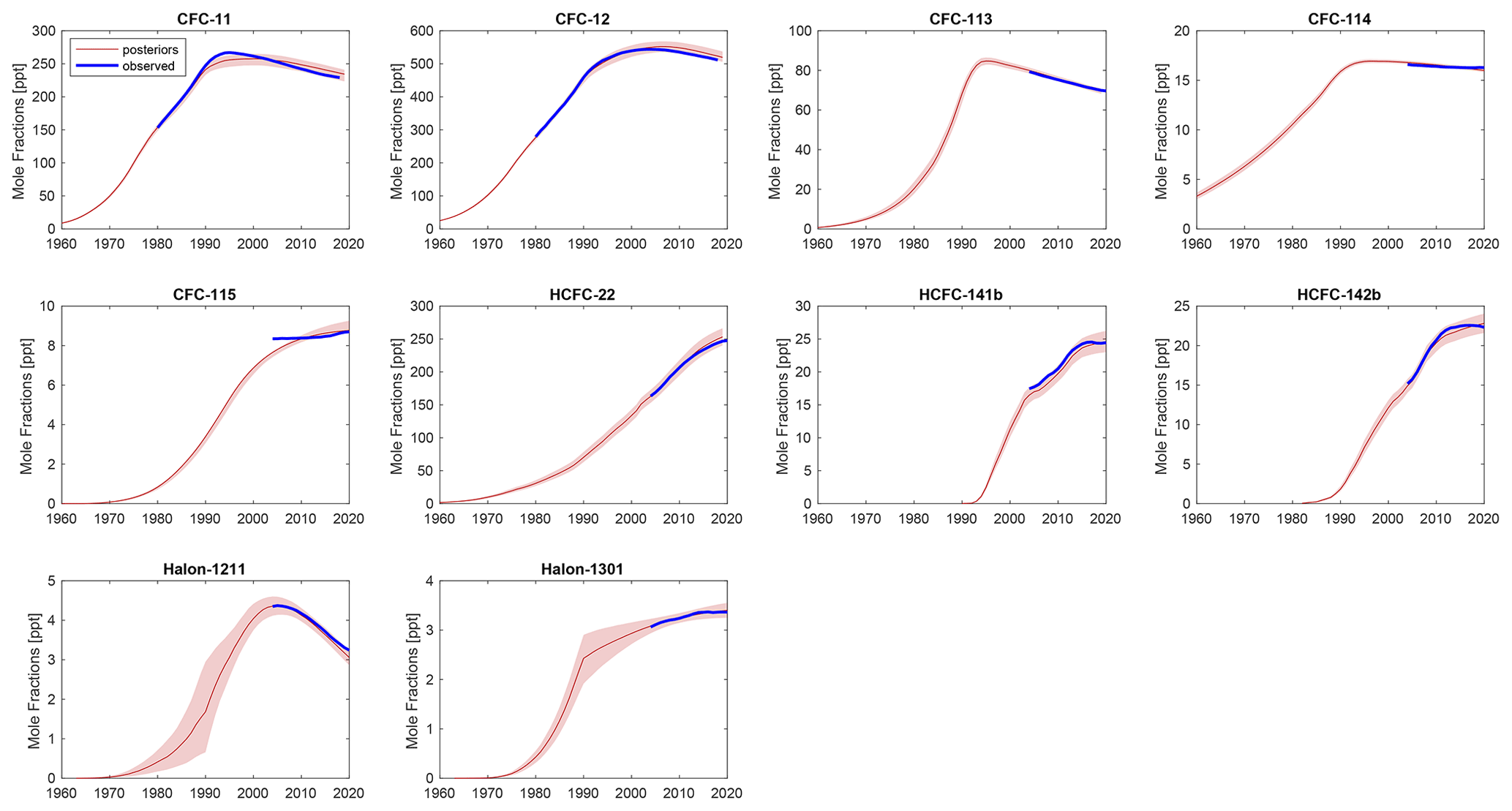
Figure 1 Modeled mole fractions versus observed mole fractions. Red lines indicate the posterior median mole fraction estimate from the Bayesian parameter estimation (BPE), with shaded regions indicating the 90 % confidence interval. Blue lines indicate globally averaged observed mole fractions.

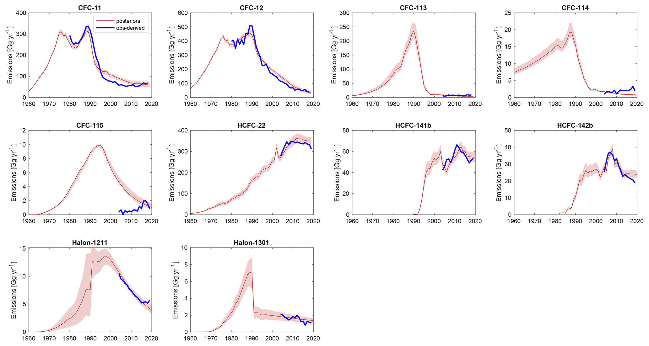
Figure 2 Modeled emissions versus observationally derived emissions. Red lines indicate the posterior median emissions estimate from the Bayesian parameter estimation (BPE), with shaded regions indicating the 90 % confidence interval. Blue lines indicate observationally derived emissions assuming the SPARC multimodel time-varying mean lifetimes.

Figure 3 provides a comparison of BPE bank estimates alongside previously published bank estimates. The BPE bank estimates are generally higher than other published values. This can be explained by production uncertainties that are accounted for in the present analysis. Our analysis suggests that production has most likely been underreported for nearly all chemicals. Table 2 provides a summary of our estimated bias in cumulative reported production throughout the simulation period for each chemical type. With the exception of CFC-113 and CFC-115, we find our inferred cumulative production to be significantly higher than reported production (at the 1-sigma level), with our median estimate suggesting that production was as little as 9 % higher than reported for CFC-12 and as high as 50 % higher than reported for halon 1211. Note, however, that high uncertainties in lifetimes for halon 1211 exist (Ko et al., 2013) and could explain part of this discrepancy. We would expect any consistent bias in reported production to be a bias low, since consistent undercounting of production is more plausible than overcounting production. The exception for this would be the base year, which reduction targets are made with reference to. In this instance, we would expect overreporting for this year to be more likely. Another possible explanation for the discrepancy in production estimates is that total reported chemical production under UNEP does not account for leakage during chemical manufacturing, but rather only leakage that occurs during the application of the chemical. To our knowledge, this potential leakage during chemical manufacturing has not been well-documented or previously quantified.

Figure 3 Magnitudes of bank estimates. The red lines indicate the median posterior estimate of banks from the Bayesian analysis, with shading indicating the 90 % confidence interval. Previously published bank estimates are provided for comparison from the 2009 TEAP report (Kuijpers and Verdonik, 2009), WMO (2007), WMO (2018) and Lickley et al. (2020) along with the hybrid approach updated to current estimated starting values.

Table 2 Estimated bias in cumulative reported production. Values indicate the percent difference between inferred cumulative production from the onset of production to 2019 relative to reported production, for all uses except feedstock production. Positive values indicate the percent by which inferred production is higher than reported.

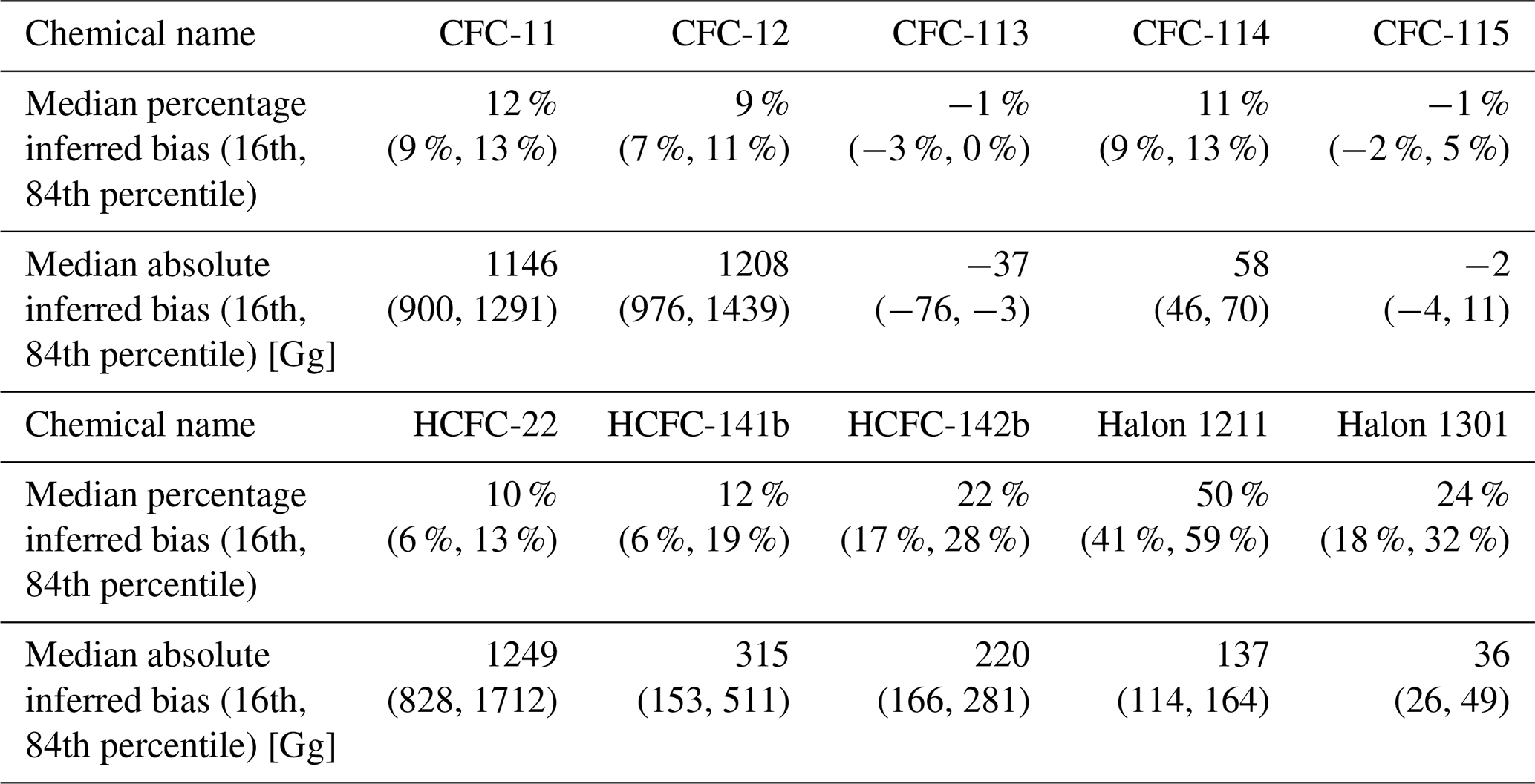
Figure 4 shows the breakdown of emissions by equipment type over time. For CFCs, emissions from short banks tend to peak around 1990, as spray applications were banned earlier than other applications, after which emissions from medium and long banks become more dominant emission sources. This is to be expected as the phase-out of production after 1990 would lead to more CFC emissions from existing banks rather than new, short-lived equipment. For HCFC-22, most of the emission throughout the entire time period is from medium banks, which is largely non-hermetic refrigeration. Long banks (i.e., foams) dominate emissions for HCFC-141b and for HCFC-142b, where both foams and non-hermetic refrigeration are prominent emission sources throughout the simulation period. Estimated feedstock emissions averaged over 2010–2019 are shown in Table 3. The HCFC-22 is the largest source of feedstock emissions by mass, but CFC-113 feedstock emissions are estimated to be larger when weighted by global warming potential (GWP100) and ODP.

Figure 4 Emissions by source – Estimates of emissions by various equipment types, summarized in Table 1, are shown here along with estimated emissions from feedstock usage. Lines indicate the median estimate, with the shaded region indicating the 90 % confidence interval. Halons are not included in this figure as 100 % of halon emissions come from the same application and are thus identical to Fig. 2 halon totals.

Table 3 Estimated feedstock emissions averaged from 2010–2019 from the Bayesian analysis. Emissions are weighted by mass, global warming potential (GWP100) relative to CO₂ over a 100-year time horizon for a CO₂ concentration of 391 ppm, and by ozone depletion potential (ODP) relative to CFC-11 (WMO, 2018).

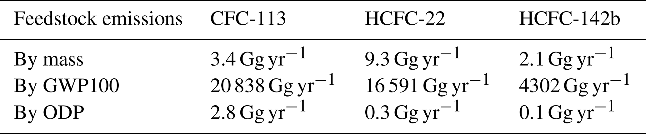
Figure 5 shows the relative quantity of banked materials by chemical type. Banks are weighted by mass (Fig. 5a), by GWP100 (Fig. 5b), and ODP (Fig. 5c). Our best estimate is that the sum of the HCFCs currently comprise about 77 % of banks by mass. However, in terms of climate impacts, CFC-11, CFC-12, and HCFC-22 are the largest banked materials weighted by GWP100, accounting for 36 %, 14 %, and 36 % of current banks, respectively. When banks are weighted by ODP, CFC-11 and CFC-12 represent 46 % and halons also represent 46 % of current banked chemicals.

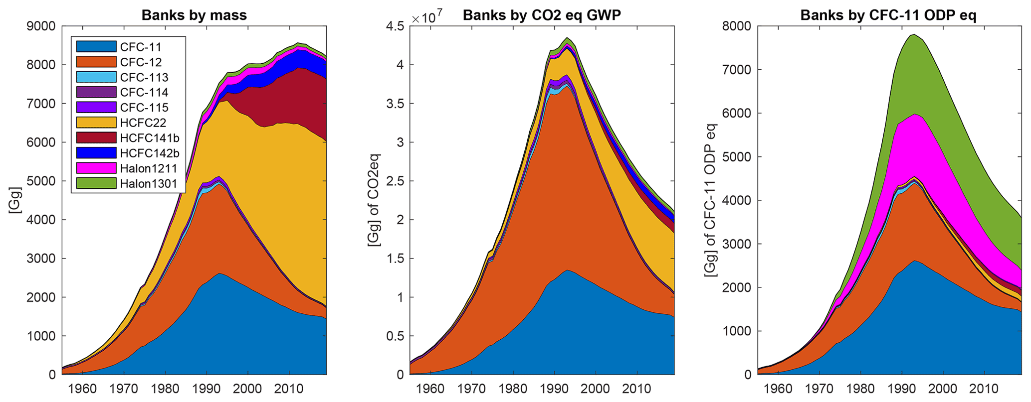
Figure 5 Total banks by mass, global warming potential (GWP100; WMO, 2018), and ozone depleting potential (ODP; WMO, 2018). Bank estimates reported in the above figures are the median estimates from the Bayesian analysis.

Figure 6 shows the composition of banks by chemical type. This, together with Fig. 5, provides insight into the most prominent banked sources of halocarbons with regards to GWP100 and ODP. In terms of GWP100, CFC-11 banks largely reside in foams, whereas CFC-12 and HCFC-22 are largely in non-hermetic refrigeration. The latter may be more readily recoverable. In terms of ODP, CFC-11 foams and CFC-12 non-hermetic refrigeration remain important, along with halons which are all contained in fire extinguishers, a recoverable reservoir.

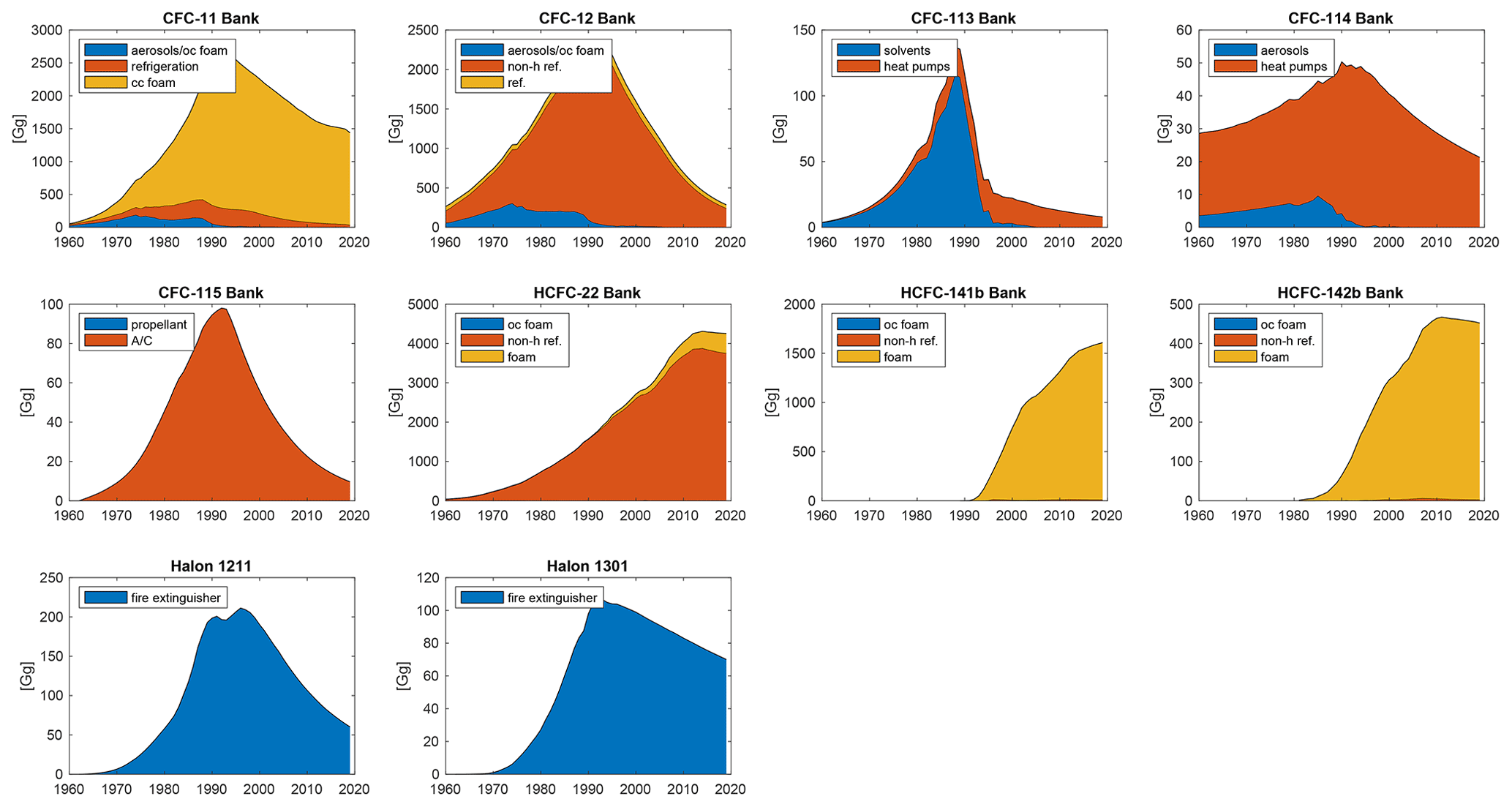
Figure 6 Bank size by equipment type. Bank estimates reported in the above figures are the median estimates from the Bayesian analysis. In the above legends, “cc” refers to closed-cell foams, “non-h ref.” refers to non-hermetic refrigeration, “ref.” refers to refrigeration, and “A/C” refers to air conditioning.

4 Discussion and conclusions

This analysis suggests that if lifetime assumptions are correct, published bank estimates using either the top-down or bottom-up approaches were likely underestimating bank sizes for all banked chemicals due to underreporting of production (see Table 2). The Bayesian approach used in this analysis does not assume that production is known precisely, but rather jointly infers production along with the other parameters in the simulation model, providing probabilistic estimates of historical production values. Previously published bank estimates (Ashford et al., 2004; Kuijpers and Verdonik, 2009; Montzka et al., 2003) do not infer production, but rather assume that it is known, or consider different scenarios. We argue that production assumptions have been biased low due to underreporting of total production and potentially unaccounted for leakage during chemical manufacturing, and thus have led to published bank estimates that were also biased low.

Discrepancies between observed mole fractions and BPE-derived mole fractions are notable for the suite of chemicals considered here. While the majority fall within the 90 % confidence interval throughout most of the time periods, the trends in concentrations between observations and inferred mole fractions do not always agree. This discrepancy could be related to our partitioning of production type following 2003 (i.e., after AFEAS data end). Another important limitation in this analysis is in the treatment of atmospheric lifetimes, which could also explain some of these discrepancies. The present analysis assumes that atmospheric lifetimes are known and equal to the SPARC report's multimodel time-varying mean lifetimes (Ko et al., 2013). However, previous work has indicated potential biases in SPARC lifetimes, for example for CFCs (Lickley et al., 2021). The potential bias in atmospheric lifetimes would result in biased bank estimates in the present paper and requires further analysis.

This modeling approach makes no assumptions about end-of-life (EOL) emissions. Certain bank estimates assume that applications are dismantled at the end of their lifetime, which would contribute to both decreased banks and increased emissions at fixed years after production (e.g., UNEP/TEAP, 2019). We do not make this assumption as we believe it would be more realistic for dismantling of equipment to occur over a range of years after production, which would effectively be captured by our bank release fraction estimate. We do however test the sensitivity of our bank estimate to EOL emissions occurring in a single year after production. This we term the EOL scenario and test the sensitivity of banks for CFC-11, CFC-12, and HCFC-22, the three largest banks by global warming potential. The modeling approach is described in the Supplement and results are shown in Fig. SM1 therein. Perhaps unexpectedly, posterior bank estimates of CFC-11 are ∼25 % higher in 2020 in the EOL scenario relative to the scenario described in the main text. However, banks in the EOL scenario are decreasing faster than those described in the main text. The larger bank size is due to posterior bank release fractions being ∼2 % for the EOL scenario relative to 3 % for the scenario described in the main text. The faster depletion of the banks in 2020 can be explained by the addition of the EOL decommissioning parameter. These larger bank estimates reflect the consistency of the Bayesian modeling approach where all parameters are jointly inferred. Including an additional process in the model requires that multiple parameters be updated to be consistent with observations. For CFC-12, the EOL scenario produces significantly smaller banks from about 1990 onwards. However, the emissions profile has an artificial dip in emissions relative to observationally derived emissions, suggesting that a set year for decommissioning is not a realistic modeling assumption. For HCFC-22, banks are not substantially different between the two scenarios.

There are important discrepancies between CFC-113 feedstock emissions inferred here and those estimated in the previous analysis (Lickley et al., 2020). In Lickley et al. (2020), feedstock emissions were assumed to be the difference between observationally derived emissions and inferred bank emissions. In the present analysis, priors of feedstock production and leakage rates are developed and feedstock emissions are then inferred. In the present analysis, observationally derived CFC-113 emissions are higher than total BPE-inferred emissions at the 1-sigma level from 2010 onwards. This suggests that either observationally derived emissions are too high, or our BPEs are too low. In Lickley et al. (2021), we find that atmospheric lifetimes of CFC-113 are most likely lower than the SPARC multimodel time-varying mean used in the present analysis. This would imply that the observationally derived emissions shown in Fig. 2 are biased low, suggesting an even larger discrepancy between BPE-inferred total emissions and observationally derived emissions. Therefore, it seems plausible that the discrepancy is due to prior feedstock emissions estimates being biased low due to larger leakage, or CFC-113 is being produced for a use that is not allowed under the Montreal Protocol.

Finally, some important details about production and destruction were not fully accounted for in this analysis. For one, feedstock priors were only included for CFC-113, HCFC-22, and HCFC-142b, which could be limiting our assessment of the sources of emissions for other chemicals. However, published feedstock values for other chemicals are not available and leakage rates in feedstock applications may be uncertain. In addition, we do not account for non-dispersive production in our analysis, namely the production of chemicals as by-products. It is possible, for example, that some of the discrepancies in CFC-115 emissions could be explained by non-dispersive emissions as identified by Vollmer et al. (2018). Moreover, we do not consider EOL destruction of equipment as there are no published records, to our knowledge, of these processes. Finally, we were not able to account for a more detailed breakdown in production by equipment type than what has been published by AFEAS, which discretizes production into, at most, four categories of equipment, and does not provide data beyond 2003. Without publicly available details of these processes, modeling of banks and emissions will continue to be limited.