Statistical and machine learning methods for evaluating trends in air quality under changing meteorological conditions

Evaluating the influence of anthropogenic-emission changes on air quality requires accounting for the influence of meteorological variability. Statistical methods such as multiple linear regression (MLR) models with basic meteorological variables are often used to remove meteorological variability and estimate trends in measured pollutant concentrations attributable to emission changes. However, the ability of these widely used statistical approaches to correct for meteorological variability remains unknown, limiting their usefulness in the real-world policy evaluations. Here, we quantify the performance of MLR and other quantitative methods using simulations from a chemical transport model, GEOS-Chem, as a synthetic dataset. Focusing on the impacts of anthropogenic-emission changes in the US (2011 to 2017) and China (2013 to 2017) on PM_2.5 and O₃, we show that widely used regression methods do not perform well in correcting for meteorological variability and identifying long-term trends in ambient pollution related to changes in emissions. The estimation errors, characterized as the differences between meteorology-corrected trends and emission-driven trends under constant meteorology scenarios, can be reduced by 30 %–42 % using a random forest model that incorporates both local- and regional-scale meteorological features. We further design a correction method based on GEOS-Chem simulations with constant-emission input and quantify the degree to which anthropogenic emissions and meteorological influences are inseparable, due to their process-based interactions. We conclude by providing recommendations for evaluating the impacts of anthropogenic-emission changes on air quality using statistical approaches.

1 Introduction

Researchers and policymakers have long been interested in understanding the anthropogenic drivers of trends in observed air pollutant concentrations in order to inform air quality policies. Declining trends in pollutant concentrations such as particulate matter with diameters less than 2.5 µm (PM_2.5) have been observed in many countries that adopted policies to limit anthropogenic emissions such as SO₂ and NO_x, including the US (McClure and Jaffe, 2018) and China (Zhang et al., 2019). As the information on anthropogenic emissions is often unavailable or very uncertain, researchers and policymakers often rely on the trends in measured air pollutants to assess the effects of policies. Attributing trends in observed concentrations to anthropogenic-emission changes requires correcting for the influence of changing meteorology, which has become increasingly important but challenging in a changing climate (Saari et al., 2019). Numerous papers attempt to use statistical methods to separate impacts of meteorology from emission changes in evaluating trends in air quality, but the performance of these commonly used statistical approaches remains unassessed. Further, the impacts of meteorological variability may not even be distinguishable from air quality trends driven by anthropogenic-emission changes, due to their interactions; the magnitude of this interaction also remains unquantified. In this paper, we devise a model-based experiment for evaluating the performance of different statistical methods used for meteorological corrections. We focus on a case of identifying emission-driven linear trends in measured concentrations of PM_2.5 and ozone (O₃), when information on the anthropogenic emission is not available.

Measured pollutant concentrations are often used as the primary basis for evaluating air quality actions. For example, in 2013, China's central government established targets that aimed to reduce annual average PM_2.5 concentrations of three urban clusters by 15 % to 25 % between 2012 and 2017 (State Council of the People's Republic of China, 2013). This later translated into a stringent and binding target of a maximum annual mean PM_2.5 concentration of 60 µg m⁻³ in 2017 for Beijing, which was ultimately reached (the 2017 concentration was 58.5 µg m⁻³) (Beijing Municipal Ecology and Environment Bureau, 2013). However, several studies estimated that the concentration would have exceeded this target in Beijing were it not for meteorological conditions in the winter 2017 that favored pollution reductions (Vu et al., 2019; Chen et al., 2019; Cheng et al., 2019). The European Union and US Environmental Protection Agency (EPA) use a 3-year average of the PM_2.5 concentration to determine compliance with air quality standards (European Union, 2020; US Environmental Protection Agency, 2019). The US EPA has also proposed to use statistical approaches that aim to correct for the impacts of weather variability on O₃ concentrations in the designation processes (Wells et al., 2021).

Many studies use multiple linear regression (MLR) models with basic meteorological variables to correct for meteorological variability in order to estimate the impacts of emission changes on measured air quality (Otero et al., 2018; Zhai et al., 2019; Li et al., 2018, 2020; Han et al., 2020; Chen et al., 2020). Zhai et al. (2019) and Li et al. (2020) use MLR models to estimate the degree to which trends in PM_2.5 and O₃ from 2013 to 2019 in China were driven by anthropogenic-emission changes. They first use MLR to predict the PM_2.5 and O₃ concentrations with meteorological variables and then interpret the residuals of the MLR model as signals resulting from emission changes. A related approach is to combine MLR with techniques that can decompose time series of observed concentrations into long-term, seasonal, and short-term components (e.g., Kolmogorov–Zurbenko (KZ) filters, Zurbenko, 1994). Ma et al. (2016) and Chen et al. (2019) use KZ filters to calculate the long-term component of observed PM_2.5 and then apply MLR to separate the impacts of long-term meteorological changes on the concentrations. Henneman et al. (2015) apply MLR to the short-term component (identified by KZ filters) of air pollutant concentrations near Atlanta during 2000 to 2012 to separate the impact of short-term meteorological variability and then estimate the long-term trend in air quality.

Other statistical methods including non-linear regression or machine learning models have also been used to correct for meteorological variability (Holland et al., 1998; Carslaw et al., 2007; Hayn et al., 2009; Vu et al., 2019). One popular method is to use a generalized additive model (GAM) to estimate non-linear smooth functions of each meteorological variable within a given smoothing-function family with penalization on non-smoothness. The US EPA uses a GAM model of temperature, wind direction and speed, humidity, pressure, stability, transport trajectories, and synoptic weather to perform weather corrections in assessing long-term trends in O₃ (Camalier et al., 2007). An increasing number of studies use machine learning models (Grange et al., 2018; Vu et al., 2019; Zhang et al., 2020; Shi et al., 2021; Qu et al., 2020). Vu et al. (2019) use a random forest model to predict pollutant concentrations in Beijing with time index and meteorological variables and then calculate the “weather-normalized” concentration for each day with 1000 sets of meteorological fields drawn from the historical meteorological data. They found that the decrease in PM_2.5 during 2013 to 2017 was largely driven by emission reductions, although the magnitude of reduction is smaller when correcting for meteorological variability.

Despite a large number of papers that apply various meteorology correction methods, very little is known about whether these methods can effectively correct for meteorological variability and thus realistically estimate the counterfactual air quality and reveal the underlying impacts of anthropogenic-emission changes. Most studies cite the prediction performance of their statistical models (such as R² and/or mean squared errors) to justify their method choice and analysis. However, good prediction performance does not guarantee the correct estimation of counterfactuals and causal effects (Runge et al., 2019). The performance of these meteorology-corrected methods is unable to be assessed using observational data alone, as the underlying emission-driven trends without influence from meteorological variability cannot be derived from data. Further, statistical analyses often assume that the influence of meteorological variability on pollutant concentration can be cleanly separated from the influence of anthropogenic-emission changes. This is not completely possible, as the impacts of meteorological variability on pollutant concentration will also vary depending on the emissions. The degree to which this interaction affects the ability to calculate emission-related trends under changing meteorology also remains unknown.

Figure 1 Overview of research methodology. Terms and coefficients are linked to the associated terms in Eq. (1) and Table 1.

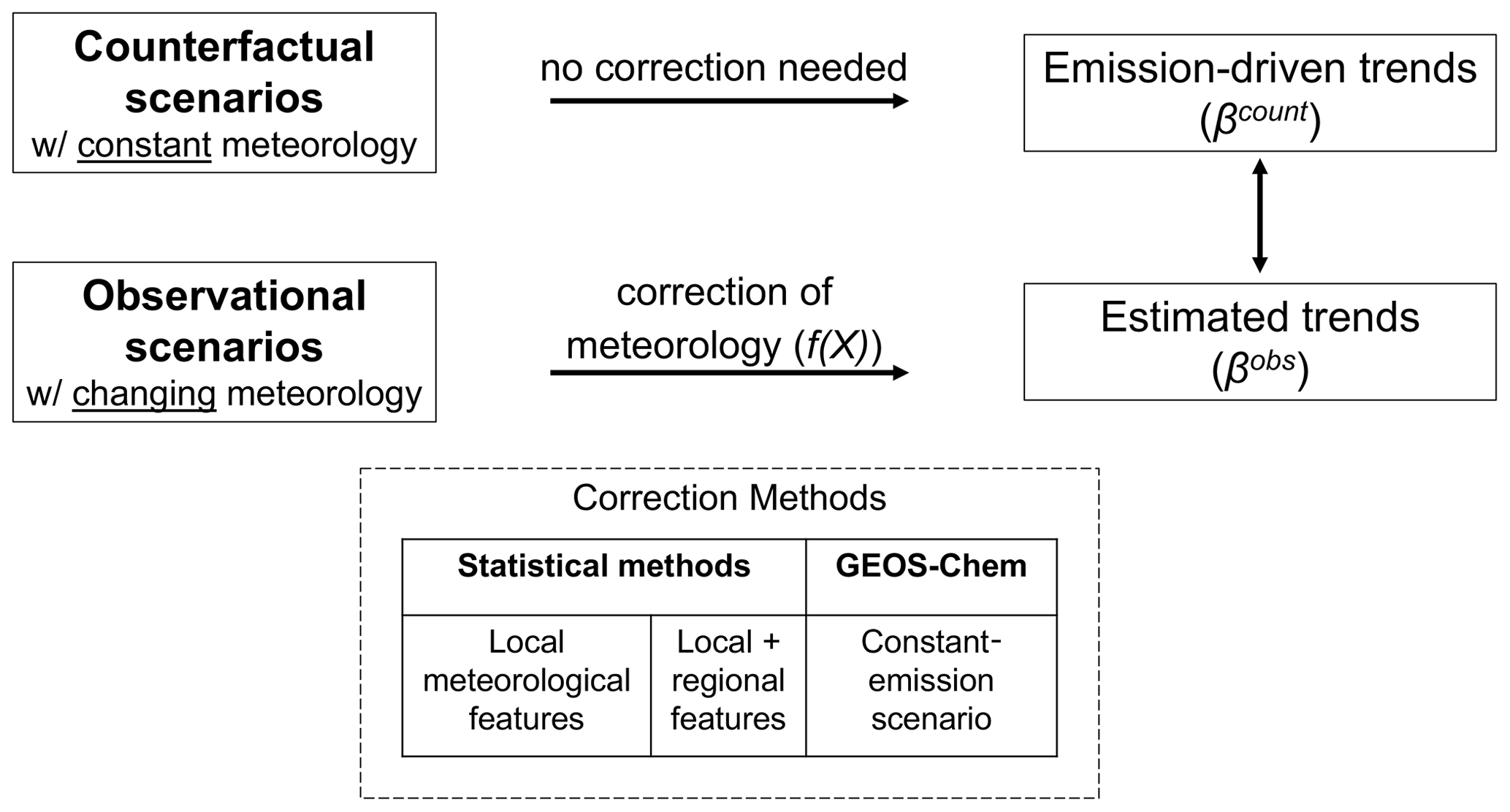
Here, we conduct a model experiment to evaluate the performance of widely used statistical models in correcting for meteorological variability and estimating emission-driven trends in air quality (see Fig. 1). We focus on the impacts of anthropogenic-emission changes on annual PM_2.5 and summer O₃ in the US (2011–2017) and China (2013–2017), two periods well-studied in previous literature. Using a three-dimensional atmospheric chemical transport model, GEOS-Chem, we simulate two sets of scenarios – “observational scenarios” with assimilated meteorological inputs (with interannual variability) and “counterfactual scenarios” with constant meteorological inputs. Using simulated daily concentrations in the observational scenarios, we estimate meteorology-corrected trends for each grid cell from regression models using different statistical correction methods. We then compare the derived trends with the emission-driven trends in the counterfactual scenarios (which are free of meteorological variability by design), calculating the resulting “error” in trend estimation. We further design a correction method based on GEOS-Chem constant-emission simulations and use it to quantify the degree to which attribution to meteorology and emissions separately is possible. Finally, we apply the different statistical correction methods to observational data from surface monitoring networks in the US and China, discussing the variability across different methods. We conclude by providing recommendations for techniques to evaluate air pollution policies under changing meteorological conditions.

2 Method

2.1 GEOS-Chem

GEOS-Chem is a global three-dimensional chemical transport model driven by assimilated meteorological data from the Goddard Earth Observation System (GEOS-5) of the NASA Global Modeling and Assimilation Office (GMAO) (Bey et al., 2001; http://www.geos-chem.org/, last access: March 2022). The simulation of PM_2.5 in GEOS-Chem represents an external mixture of secondary inorganic aerosols, carbonaceous aerosols, sea salt, and dust aerosols. GEOS-Chem includes detailed O₃–NO_x–volatile organic carbon (VOC)–aerosol–halogen tropospheric chemistry (Travis et al., 2016; Sherwen et al., 2016). The GEOS-Chem model has been previously used to study the changes in PM_2.5 and O₃ during our studied periods, and model simulations have been shown to be consistent with the observed concentrations (see, e.g., C. Li et al., 2017; Xie et al., 2019, for the US, and Li et al., 2018; Lu et al., 2019; Zhai et al., 2021, for China). Studies in both regions show that the GEOS-Chem model is able to reproduce the spatial, seasonal, and interannual variability and the long-term trends in observed pollutant concentrations, despite biases in absolute concentrations in certain species and regions (Heald et al., 2012; Travis et al., 2016; Tian et al., 2021).

We use GEOS-Chem version 12.3.0 with a horizontal resolution of ${\mathrm{0.5}}^{\circ }\times \mathrm{0.625}$^∘ in North America and Asia (Wang et al., 2004). For each scenario, we first conduct a global run at a horizontal resolution of ${\mathrm{4}}^{\circ }\times \mathrm{5}{}^{\circ }$, with a 12-month spin-up. These global runs are then used as the boundary conditions for nested simulations in the US and China with finer resolution of ${\mathrm{0.5}}^{\circ }\times \mathrm{0.625}{}^{\circ }$.

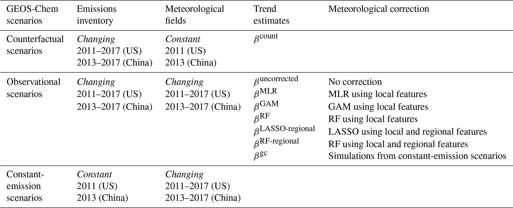
Table 1 Overview of GEOS-Chem scenarios and meteorological correction methods. RF: random forest. LASSO: least absolute shrinkage and selection operator.

2.2 GEOS-Chem scenarios

Table 1 shows the simulations included in our model experiments. We simulate two sets of scenarios – observational scenarios with interannual variability in meteorology and counterfactual scenarios with constant meteorological inputs. Both scenarios use the same emission inventory as input (see Sect. 2.3). For each grid cell, we estimate the linear trends in pollutant concentrations from simulated daily PM_2.5 and O₃ concentrations. We focus on the daily 24 h average PM_2.5 over all seasons and the maximum daily average 8 h (MDA8) O₃ in summer (June, July, August). Our focus on the 3 summer months is consistent with many previous studies (e.g., Shen et al., 2015), although this may not capture the peak ozone season for certain regions of the US and China. Our GEOS-Chem simulations use meteorological fields from the Modern-Era Retrospective analysis for Research and Applications, Version 2 (MERRA-2) (Gelaro et al., 2017). We aggregate the hourly meteorological data for consistency with the pollutant concentrations: a 24 h average for PM_2.5 analysis and the corresponding 8 h average for O₃. Meteorological features that are used in the statistical models can be found in Sect. 2.4.

2.2.1 Observational scenarios

Observational scenarios simulate PM_2.5 and O₃ under changing emissions and changing meteorological fields. Trends estimated under the observational scenarios (β^obs) are subject to the influences of interannual meteorological variability. Our model experiments were not specifically designed to reproduce observed air quality in these two regions but rather to provide a realistic test case to evaluate the performances of statistical methods. Nevertheless, as shown in Figs. S1 and S2 in the Supplement, the simulated concentrations in PM_2.5 and O₃ largely reproduce the daily variability in observed pollutant concentrations. The linear trends in simulated PM_2.5 and O₃ concentrations in the observational scenario are largely consistent with trends of the measured concentrations. For example, the average trend (±1 standard deviation) in the US is −0.27 ± 0.30 $\mathrm{\mu }{\mathrm{g}}^{-\mathrm{3}}{\mathrm{yr}}^{-\mathrm{1}}$ (observation) and −0.39 ± 0.24 ppb yr⁻¹ (GEOS-Chem) for PM_2.5 and −0.91 ± 0.98 ppb yr⁻¹ (observation) and −1.02 ± 0.83 ppb yr⁻¹ (GEOS-Chem) for O₃. The only exception is that our model cannot reproduce the increasing PM_2.5 trends in the Northwest US because we do not consider interannual variability in biomass-burning emissions.

2.2.2 Counterfactual scenarios

Counterfactual scenarios simulate PM_2.5 and O₃ under changing emissions but constant meteorology. All simulation years in the counterfactual scenario use the meteorological fields of the start year (2011 for the US, 2013 for China). Trends estimated under the counterfactual scenario (β^count) are not subject to interannual meteorological variability; we use this as a proxy for the trends in pollutant concentrations driven by emission changes alone. In a sensitivity analysis, we also simulate the counterfactual scenario for China using the meteorological fields for the end year, 2017 (at $\mathrm{4}{}^{\circ }\times \mathrm{5}{}^{\circ }$ resolution, due to computational constraints). We find that the linear trend in PM_2.5 and O₃ for each grid cell is highly consistent in the counterfactual scenarios across the choice of the meteorological years (see Fig. S5).

2.2.3 Assumptions for GEOS-Chem experiments

It is important to note that we do not assume our GEOS-Chem simulations perfectly represent the underlying pollutant concentration in the real world (although the model compares relatively well with the observational data). Rather, our main focus is to evaluate how different statistical methods can explain the differences between the observational and counterfactual scenarios. The assumption here is that the differences between observational and counterfactual scenarios are useful approximations of the impacts of meteorological variability on pollutant concentrations. The implications of uncertainty in GEOS-Chem for our results can be found in the “Discussion” section.

2.3 Emission inventory

For the US, we use the National Emissions Inventory 2011 (NEI 2011) as a baseline emission inventory and scale the emissions in 2012 to 2017 to match the annual total emissions each year (US Environmental Protection Agency, 2021b). For China, we use the monthly Multi-resolution Emission Inventory for China (MEIC) during 2013 to 2017 (M. Li et al., 2017; Zheng et al., 2018). During the studied time periods, the US and China experienced dramatic decreases in anthropogenic emissions, particularly in SO₂ and NO_x. In the US, total anthropogenic emissions of SO₂ decreased by 57 % and NO_x emissions decreased by 26 % during 2011 to 2017 (see Fig. S3). In China, anthropogenic SO₂ emissions decreased by 59 %, and NO_x emissions decreased by 21 % during the 2013–2017 period (see Fig. S4).

Natural emissions of multiple chemical species are calculated online in the simulations (rather than prescribed) in the GEOS-Chem model and thus can be influenced by meteorological variability (see Keller et al., 2014, for more details). Impacts of meteorology on PM_2.5 and O₃ concentrations through changes in the natural emissions are considered here as part of the meteorology–concentration relationship. These emissions include NO_x emissions from lightning and soil processes, sea salt emissions, dust emissions, and biogenic volatile organic carbon (VOC) emissions. However, biomass-burning emissions are prescribed in the GEOS-Chem model, and we hold them constant at the level of the start year. We make this simplification because the GEOS-Chem model uses biomass-burning emissions from external inventories such as the Global Fire Emissions Database (van der Werf et al., 2017), and it is impossible to distinguish natural fire emissions (part of the meteorological variability) from anthropogenic fire emissions (e.g., from farm residual burning). The role of natural emission changes in the meteorology–air quality relationship is further expanded on in the “Discussion” section.

2.4 Statistical and machine learning models

2.4.1 Model with local meteorological variables

We assess the performance of statistical and machine learning models to correct for the meteorological variability in the observational scenarios. We evaluate these methods with a commonly used framework (e.g., used in Li et al., 2018, and Zhai et al., 2019) which models the air pollutant concentrations of each individual grid cell using an additive form of a trend component, a meteorology component, and time fixed effects (to capture daily and monthly variability not related to meteorology). More specifically, we estimate the following regression equation for each grid cell i:

$$\begin{array}{}\text{(1)}& y_{it}={\mathit{\beta }}_i^{\text{obs}}\times t+f_i\left(X_{it}\right)+{\mathit{\eta }}_{it}+{\mathit{ϵ}}_{it},\end{array}$$

where y_it denotes the PM_2.5 or O₃ concentration at grid cell i on day t. t is the time index (e.g., in the US, t=1 for 1 January 2011 and t=2 for 2 January 2011). X_it denotes the local meteorology features (i.e., meteorological variables in grid cell i on day t). η_it is the month-of-year × day-of-month fixed effect to capture daily and monthly variability in pollutant concentrations that are not related to the meteorological variability (e.g., seasonal cycle in O₃ and PM_2.5). ϵ_it is the normally distributed error term. ${\mathit{\beta }}_i^{\text{obs}}$ represents the meteorology-corrected trend in PM_2.5 or O₃ concentration for grid cell i estimated with the standard ordinary least-squares method. We use the absolute differences $|{\mathit{\beta }}_i^{\text{obs}}-{\mathit{\beta }}_i^{\text{count}}|$ to evaluate the performance of different methods to correct for meteorological variability for any given grid cell i.

Here, f_i(X_it) represents the specifications of local meteorological features for grid cell i under different methods. In addition to the commonly used multiple linear regression (MLR) model, we also evaluate the following models with higher flexibility: polynomial regression models (quadratic, cubic), cubic spline models, generalized additive models (GAM, implemented with R package “mgcv” by Wood, 2011), and random forest (RF) models. We refer to the trend estimates estimated without f_i(X_it) as uncorrected. We focus on the methods in Table 1 in the main text, and the performance of the other methods can be found in Tables S1 and S2 in the Supplement. Note that the time fixed effects are modeled differently in RF models due to the estimation procedure. More details on the implementation of RF can be found in the Supplement.

We use the following 10 variables from MERRA-2 as our selected meteorological features for the statistical analysis: surface temperature, precipitation, humidity, planetary boundary layer height, cloud fraction, surface air pressure, and wind speed (U and V direction, at surface and 850 hPa levels). These variables are the most commonly used features in previous studies. We also perform sensitivity analyses that include nine more meteorological features: direct photosynthetically active radiation, diffuse photosynthetically active radiation, tropopause pressure, friction velocity, topsoil moisture, root soil moisture, snow depth, surface albedo, and surface air density. These features are selected because they are used as primary or intermediate inputs for calculating PM_2.5 or O₃ concentrations in the GEOS-Chem model and may be relevant for the variability in pollutant concentrations.

2.4.2 Model with local and regional meteorological variables

We also evaluate models that use both local and regional meteorological features. Regional meteorological features are important for explaining variability in local pollutant concentrations due to (1) pollution transport from neighboring locations and (2) influences from meteorological systems at the synoptic scale (i.e., large-scale weather systems that span over 1000 km such as circulation patterns) (Tai et al., 2012; Shen et al., 2015; Zhang et al., 2018; Leung et al., 2018; Han et al., 2020). As the incorporation of both local and regional features can quickly expand the dimensionality of the feature space, here we use the least absolute shrinkage and selection operator (LASSO) and the random forest (RF) model, two statistical models that show good prediction performances with high-dimensional data inputs. We estimate the following equations:

$$\begin{array}{}\text{(2)}& y_{it}={\mathit{\beta }}_i^{\text{obs}}\times t+g_i(X_{it},Z_t)+{\mathit{\eta }}_{it}+{\mathit{ϵ}}_{it},\end{array}$$

where g_i() denotes the functional form fitted by LASSO or RF. X_it again denotes the local meteorology features for grid cell i on day t. Z_t denotes the regional-scale meteorology features including the meteorological features for every grid cell in the US on day t (98 cells in $\mathrm{4}{}^{\circ }\times \mathrm{5}{}^{\circ }$; we choose a relatively coarse resolution due to computational cost). Meteorological information in each location in the US may help explain the pollutant concentrations in grid cell i. In total, we have 10 local features (X_it) and $\mathrm{10}\times \mathrm{98}=\mathrm{980}$ regional-scale features (Z_t). The coefficient ${\mathit{\beta }}_i^{\text{obs}}$ is obtained with the double machine learning approach by Chernozhukov et al. (2018). In particular, the hyperparameters and coefficients of LASSO and RF are selected and fitted using 4-fold cross-validation to avoid the “overfitting risk”. More details on the implementation of LASSO and RF can be found in the Supplement.

2.5 Correction approach using the GEOS-Chem constant-emission scenario

We further design and evaluate an approach to correct for meteorology variability with GEOS-Chem simulations (referred to as the “constant-emis” approach). The constant-emis approach uses GEOS-Chem simulations with constant anthropogenic emissions and changing meteorological fields (“constant-emission scenarios” in Table 1). All years in the constant-emission scenario use anthropogenic emissions of the start year (2011 for the US, 2013 for China). Note that the constant-emis approach also aims to estimate meteorology-corrected trends from the simulated concentrations in the observational scenario. We estimate the following equations:

$$\begin{array}{}\text{(3)}& y_{it}={\mathit{\beta }}_i^{\text{gc}}\times t+{\text{SIM}}_{it}+{\mathit{\eta }}_{it}+{\mathit{ϵ}}_{it},\end{array}$$

where y_it denotes the simulated concentrations in the observational scenario, SIM_it denotes the simulated concentrations on day t in grid cell i in the constant-emission scenarios. SIM_it serves a similar purpose as the term “f_i(X_it)” in Eq. (1) but comes from the GEOS-Chem simulation. Some previous studies have also used model simulations with constant-emission input as a way to characterize meteorological variability (Zhong et al., 2018; Zhao et al., 2020). ${\mathit{\beta }}_i^{\text{gc}}$ is the estimated meteorology-corrected trend for PM_2.5 or O₃ concentration using this model-based correction method.

Compared to previous statistical and machine learning approaches, the constant-emis approach better captures the meteorological variability as simulated in GEOS-Chem (as SIM_it is directly taken from GEOS-Chem). Therefore, the difference between the trend estimates (β^gc) and counterfactual trends (β^count) provides a conceptual minimum for estimation errors using the framework of Eq. (1) to perform meteorological corrections. The commonly used framework of Eq. (1) assumes that the impacts of meteorology variability can be separated from the impacts of anthropogenic emissions. In our experiments, this assumption indicates that the differences between the counterfactual scenario and the observational scenario can be solely explained by the meteorological variables. However, the difference in pollutant concentrations between these scenarios is also in part driven by emissions in their interaction with meteorology (despite the fact that our different scenarios use the same emission inventory). We use $|{\mathit{\beta }}_i^{\text{gc}}-{\mathit{\beta }}_i^{\text{count}}|$ to quantify the estimation error associated with ignoring such interactions in this framework.

2.6 Air quality observation data

We use the surface air quality measurements from the Air Quality System administered by the US EPA (US Environmental Protection Agency, 2021a). We use the daily 24 h average of PM_2.5 concentrations for all months and the daily maximum 8 h average (MDA8) O₃ concentrations for June, July, and August. Figure S1 shows the locations, trends in measured concentrations, and correlations between GEOS-Chem simulations and measured concentrations.

The surface air quality measurements in China are derived from the monitoring network administered by China's Ministry of Ecology and Environment (2021). The monitoring network was launched in 2013 and has expanded to all prefecture-level cities in mainland China. We use the daily 24 h average of PM_2.5 concentrations and the MDA8 O₃ concentrations for summer. Figure S2 shows the locations, trends in measured concentrations, and correlations between GEOS-Chem simulations and measured concentrations.

We use the meteorological variables from MERRA-2 when performing meteorology corrections at these monitoring stations because the meteorology information is not available for all these variables at the station level. This is consistent with previous analyses estimating the meteorology-corrected trends using observational air quality data (e.g., Li et al., 2018).

3 Results

3.1 Performance of different correction methods: US (2011–2017)

Figure 2a and c show the trends in PM_2.5 and O₃ concentrations in the counterfactual scenarios in the US. When holding meteorological fields constant across years, decreasing trends in the simulated PM_2.5 concentrations across the US result from decreasing anthropogenic emissions. The counterfactual scenario also shows negative linear trends in O₃ concentrations in all but three grid cells in the western US. Increases in summer O₃ in these locations result from the non-linear relationship between O₃ concentrations and NO_x emissions.

Figure 2 Trend estimates of daily annual PM_2.5 (a, b) and summer O₃ (c, d) in the US. Panels (a) and (c) show trend estimates under the counterfactual scenario (β^count). Panels (b) and (d) show the absolute magnitude of errors in trend estimates under different correction methods compared with the counterfactual scenarios ($|{\mathit{\beta }}^{\text{obs}}-{\mathit{\beta }}^{\text{count}}|$). The average of the absolute errors for each method is shown in the figure (unit of trend estimate: $\mathrm{\mu }\mathrm{g}{\mathrm{m}}^{-\mathrm{3}}{\mathrm{yr}}^{-\mathrm{1}}$ for PM_2.5 and ppb yr⁻¹ for O₃).

Figure 2b and d show the degree to which different meteorological correction methods can recover the emission-driven trends in the counterfactual scenarios. When no correction for meteorology is performed (“uncorrected” in Fig. 2b), we observe large estimation errors in trend estimates over the northeastern and southern US by up to 0.25 $\mathrm{\mu }\mathrm{g}{\mathrm{m}}^{-\mathrm{3}}{\mathrm{yr}}^{-\mathrm{1}}$, an error that is 50 % of the counterfactual trends. We find that the widely used MLR method does not help reduce these errors in PM_2.5 trend attributions. MLR has a modest impact on reducing the errors in the northeastern US, but it does not decrease the errors over the southern US and leads to even higher errors over the midwestern US. Nationwide, the average magnitude of errors (relative to the counterfactual scenario) increases with the MLR correction (0.083 $\mathrm{\mu }\mathrm{g}{\mathrm{m}}^{-\mathrm{3}}{\mathrm{yr}}^{-\mathrm{1}}$) compared to the uncorrected case (0.066 $\mathrm{\mu }\mathrm{g}{\mathrm{m}}^{-\mathrm{3}}{\mathrm{yr}}^{-\mathrm{1}}$). Among the five methods, we find that the RF model using both local- and regional-scale features (“RF-regional” in Fig. 2) offers the best performance in recovering the trends in the counterfactual scenarios and is the only method that yields smaller errors than the uncorrected case (the nationwide average error decreased by 0.019 $\mathrm{\mu }\mathrm{g}{\mathrm{m}}^{-\mathrm{3}}{\mathrm{yr}}^{-\mathrm{1}}$; 28 % less). The RF-regional model also outperforms the RF-local and LASSO-regional models, suggesting the importance of considering non-linearity, interactions between different meteorological features, and regional meteorology information in correctly adjusting for the impacts of meteorology.

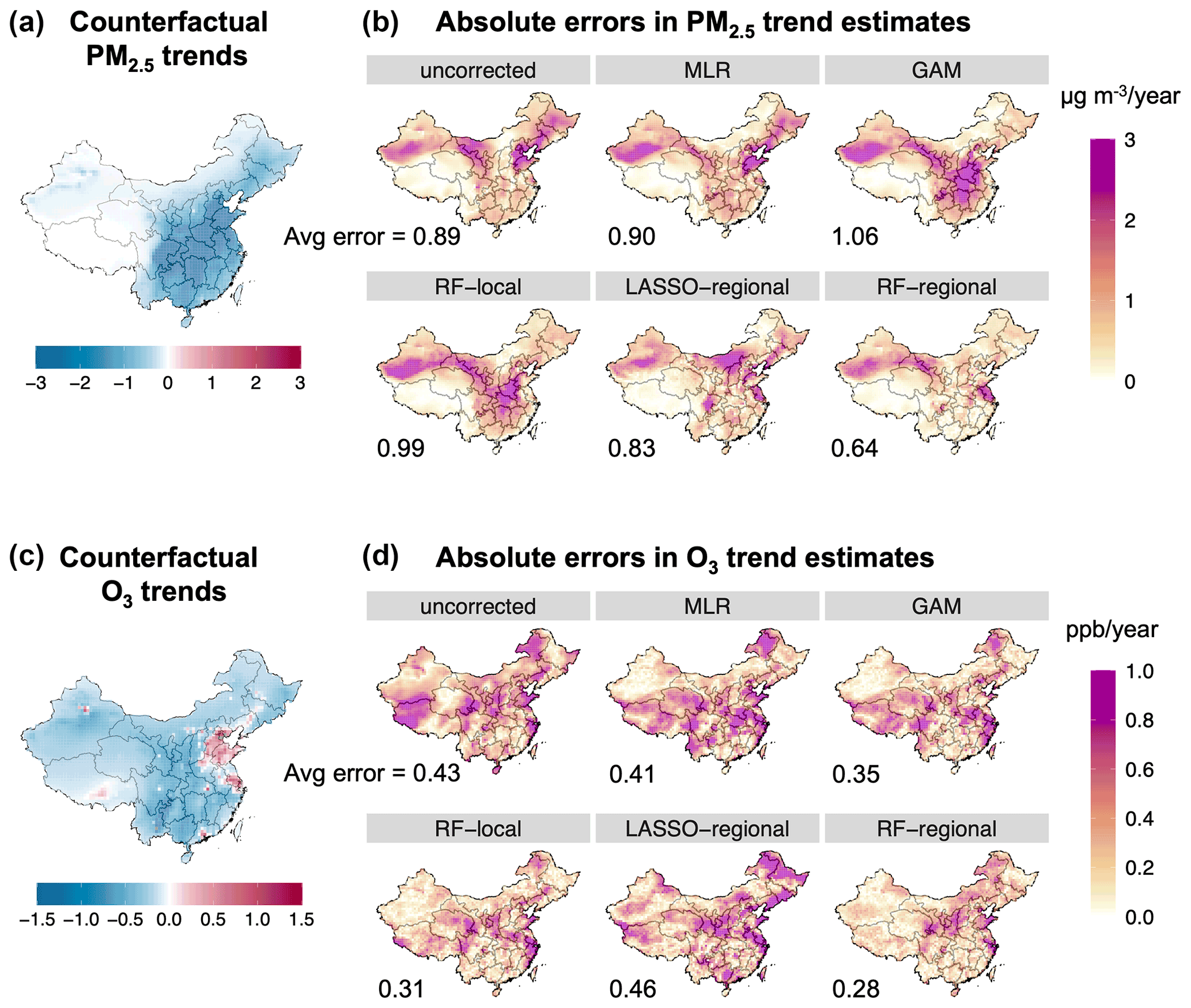
Figure 3 Trend estimates of daily annual PM_2.5 (a, b) and summer O₃ (c, d) in China. Panels (a) and (c) show trend estimates under the counterfactual scenario (β^count). Panels (b) and (d) show the absolute magnitude of errors in trend estimates under different correction methods compared with the counterfactual scenarios ($|{\mathit{\beta }}^{\text{obs}}-{\mathit{\beta }}^{\text{count}}|$). The average of the absolute errors for each method is shown in the figure (unit of trend estimate: $\mathrm{\mu }\mathrm{g}{\mathrm{m}}^{-\mathrm{3}}{\mathrm{yr}}^{-\mathrm{1}}$ for PM_2.5 and ppb yr⁻¹ for O₃).

Meteorological variability also has a substantial influence on the summertime O₃ trends in the US during this period (as shown in Fig. 2d). Relative to the counterfactual scenario, the uncorrected O₃ trends are biased by over 1–2 ppb yr⁻¹ in large areas of California, the Midwest and South US (as much as 320 % of the counterfactual trends). This is largely driven by the fact that the 2011 and 2012 summers were particularly hot in these regions and led to higher concentrations of O₃ at the beginning of this 7-year period (see Fig. S7 for the South and Midwest US). Therefore, failure to correct for meteorological variability results in much more negative trend estimates in the O₃ concentrations in these areas compared to the counterfactual scenario (see Fig. S6). Meteorology corrections with MLR or GAM help reduce these estimation errors substantially (nationwide average error is reduced by 51 % using MLR or 57 % using GAM compared to uncorrected trends), while large errors still persist in the Midwest and South US. Similar to the case of PM_2.5, the RF-regional model offers the best performance in correcting for meteorological variability (the national average error is further reduced by 42 %, compared to MLR), and it is especially helpful in reducing the errors over the Midwest and South US (regional average error is reduced by 64 % and 44 %, respectively, compared to MLR).

3.2 Performance of different correction methods: China (2013–2017)

Figure 3a and c show the trends in PM_2.5 and O₃ concentrations in the counterfactual scenarios in China. We find a substantial decline in simulated PM_2.5 concentration during 2013 to 2017, particularly in eastern and central China. In contrast, there is little change in the simulated PM_2.5 concentrations in western China in the counterfactual scenario, where PM_2.5 is dominated by dust species largely driven by natural processes (see Fig. S9). For summer O₃, there are decreasing trends in the counterfactual scenario in most parts of China, except for northern China and some urban areas. This is largely consistent with previous studies that attempt to attribute emission-related changes in O₃ concentrations during this period based on modeling or observational data (Li et al., 2018, 2020; Lu et al., 2020).

Figure 3b shows the magnitude of estimation errors in the trend estimates of annual PM_2.5 in China under different correction methods. We find the underlying meteorological variability has a substantial impact on PM_2.5 trends in China during this period. We observe large differences between the uncorrected and counterfactual trends in simulated PM_2.5 concentrations, particularly in Northwest and Northeast China. Similar to the model experiments in the US, we find that MLR and GAM methods fail to correct for this underlying meteorological variability and lead to further increases in estimation errors in many locations. Relative to the counterfactual scenario, the nationwide average error increases to 0.90 $\mathrm{\mu }\mathrm{g}{\mathrm{m}}^{-\mathrm{3}}{\mathrm{yr}}^{-\mathrm{1}}$ with MLR and 1.06 $\mathrm{\mu }\mathrm{g}{\mathrm{m}}^{-\mathrm{3}}{\mathrm{yr}}^{-\mathrm{1}}$ with GAM (compared to 0.89 $\mathrm{\mu }\mathrm{g}{\mathrm{m}}^{-\mathrm{3}}{\mathrm{yr}}^{-\mathrm{1}}$ with no correction). We find that the RF-regional model recovers the counterfactual trends better than other methods (nationwide average error: 0.64 $\mathrm{\mu }\mathrm{g}{\mathrm{m}}^{-\mathrm{3}}{\mathrm{yr}}^{-\mathrm{1}}$; an improvement of 30 % relative to MLR), but it is still not able to correct for the persistent estimation errors over Northwest China. We further analyze the performance of correction methods for the different component species of PM_2.5. As shown in Figs. S10 and S11, the MLR model is particularly unable to correct for the impacts of meteorological variability on nitrate and dust species. Compared with MLR, the RF-regional model better corrects for the impacts of meteorology on secondary organic aerosol species in southern and central China and ammonium in Northeast China but only yields modest improvement in correcting for the errors in dust concentrations over Northwest China (see Fig. S12). In a sensitivity analysis, we use an approach that first fits RF-regional models of each individual PM_2.5 species and then combines predictions for each species to derive trend estimates. The results are largely similar to the main approach that directly fits the total PM_2.5 concentration (see Fig. S13).

Figure 3d shows the magnitude of errors in the trend estimates for summer O₃ under different correction methods in China. We find that the MLR model only modestly reduces the estimation errors compared to the uncorrected cases, and the RF-regional model offers the best overall performance. The nationwide average error is reduced to 0.28 ppb yr⁻¹ using the RF-regional model (relative to 0.43 ppb yr⁻¹ uncorrected and 0.41 ppb yr⁻¹ with MLR). Similar to the evaluation of summer time O₃ in the US, we find the non-linear models (GAM, RF-local) perform better than MLR but are not as good as the RF-regional model. Surprisingly, the LASSO-regional model performs the worst in recovering the counterfactual trends. Compared to the US case, we find that the impacts of meteorological variability on O₃ and the method performances are much more spatially heterogeneous (see Figs. S6 and S8), which may be partially due to the more heterogeneous O₃ regimes in China during this period.

3.3 Limitations in separating meteorological and emission influence: quantified with constant-emission scenarios

In our model experiments in both the US and China, we find large differences remain between the trends evaluated with statistical models (even the best-performing RF-regional model) and counterfactual trends. The remaining differences could result from two different factors: (1) the statistical model cannot capture the complex relationship between meteorology and pollutant concentrations, and/or (2) the differences between the observational scenarios and counterfactual scenarios depend on not only the meteorological variability but also the anthropogenic emissions in their interaction with meteorology (i.e., impacts of meteorology on air quality also depend on the level of emissions).

We quantify the potential magnitude of this second factor using our constant-emis approach. As the constant-emis approach captures the exact relationship between meteorology and pollutant concentrations in GEOS-Chem, the error in the constant-emis approach is only associated with the second factor above and thus provides a conceptual minimum of the estimation errors that can be achievable by any statistical approach. Figure 4 shows the estimation errors in trend estimates using the constant-emission scenarios simulated by GEOS-Chem. We focus on the trends in summer O₃ in the US and annual PM_2.5 in China, for which we see the largest impacts of meteorological variability on the pollutant trends and the largest improvements in reducing estimation errors from the correction methods. Compared to the statistical models (e.g., MLR and RF-regional in Fig. 4a and c), trends evaluated using the constant-emis approach are very similar to the trends in the counterfactual scenarios. The national average error in trend estimates is only 0.04 ppb yr⁻¹ for the O₃ trends in the US (relative to 0.33 ppb yr⁻¹ under MLR or 0.19 ppb yr⁻¹ under RF-regional) and only 0.08 $\mathrm{\mu }\mathrm{g}{\mathrm{m}}^{-\mathrm{3}}{\mathrm{yr}}^{-\mathrm{1}}$ for the PM_2.5 trends in China (relative to 0.91 $\mathrm{\mu }\mathrm{g}{\mathrm{m}}^{-\mathrm{3}}{\mathrm{yr}}^{-\mathrm{1}}$ under MLR or 0.64 $\mathrm{\mu }\mathrm{g}{\mathrm{m}}^{-\mathrm{3}}{\mathrm{yr}}^{-\mathrm{1}}$ under RF-regional).

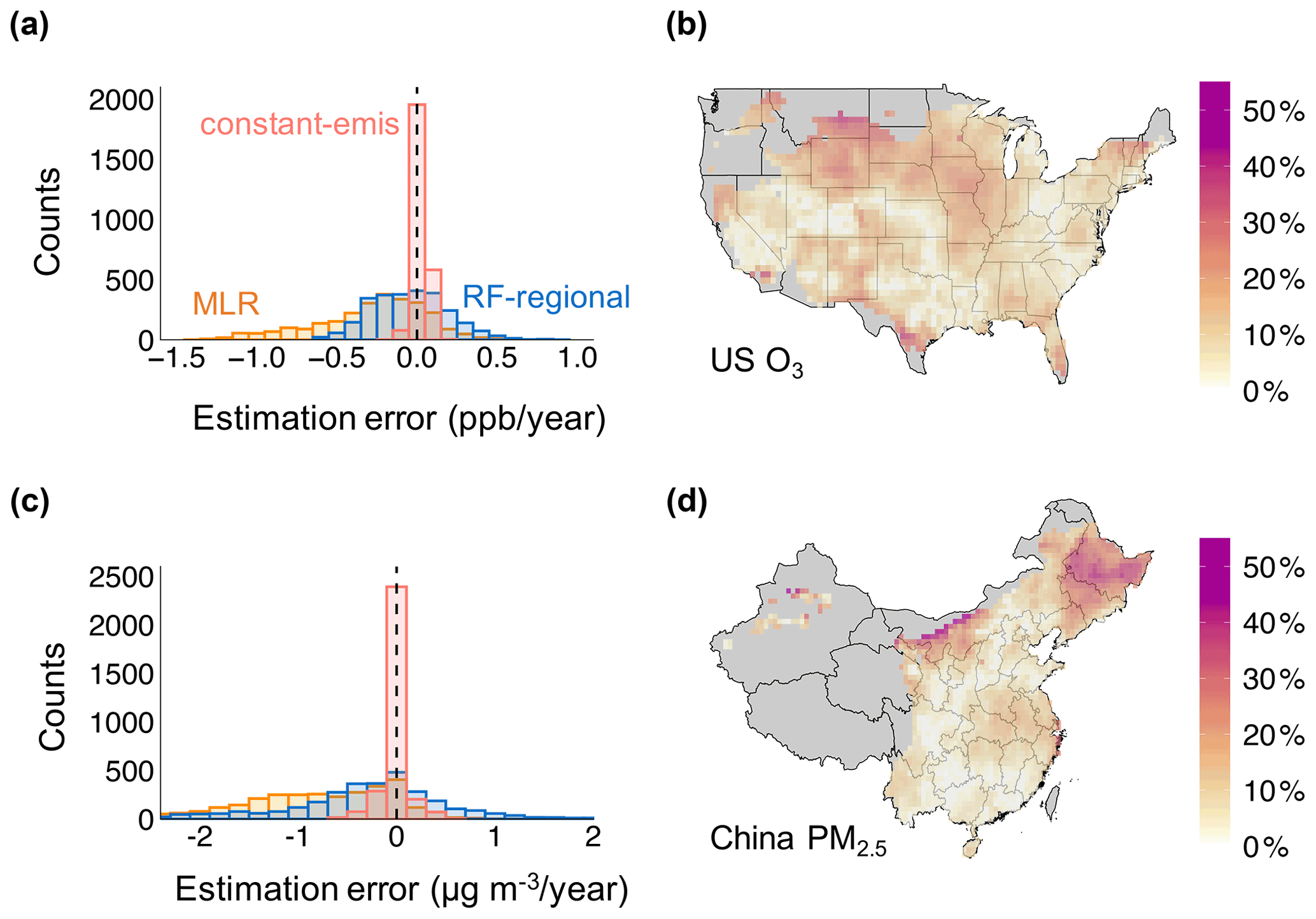
Figure 4 Panels (a) and (c) show the histogram of estimation errors in trend estimates assessed using MLR, RF-regional and constant-emis. Panels (b) and (d) show the errors assessed with the constant-emis method as a percentage of the trends in the counterfactual scenario ($|{\mathit{\beta }}^{\text{gc}}-{\mathit{\beta }}^{\text{count}}|/\left|{\mathit{\beta }}^{\text{count}}\right|$). Panels (b) and (d) only show grid cells with a trend in the counterfactual scenarios >0.2 ppb yr⁻¹ or >0.2 $\mathrm{\mu }\mathrm{g}{\mathrm{m}}^{-\mathrm{3}}{\mathrm{yr}}^{-\mathrm{1}}$; remaining grid cells are shown in gray. Panels (a) and (b) illustrate the summer O₃ trends in the US. Panels (c) and (d) illustrate the annual PM_2.5 trends in China.

However, the estimation errors calculated above are still non-negligible and can be large in certain regions. As shown in Fig. 4b and d, the constant-emis approach generally yields trend estimates biased by 10 % relative to the counterfactual trends, but the errors can be up to 40 % in certain areas. This error term is the result of ignoring how emissions could potentially influence the impacts of meteorology on the pollutant concentrations – that is, the impacts of the same meteorological variability on concentrations may be different in the start year (with high emissions) compared to the end year (with low emissions).

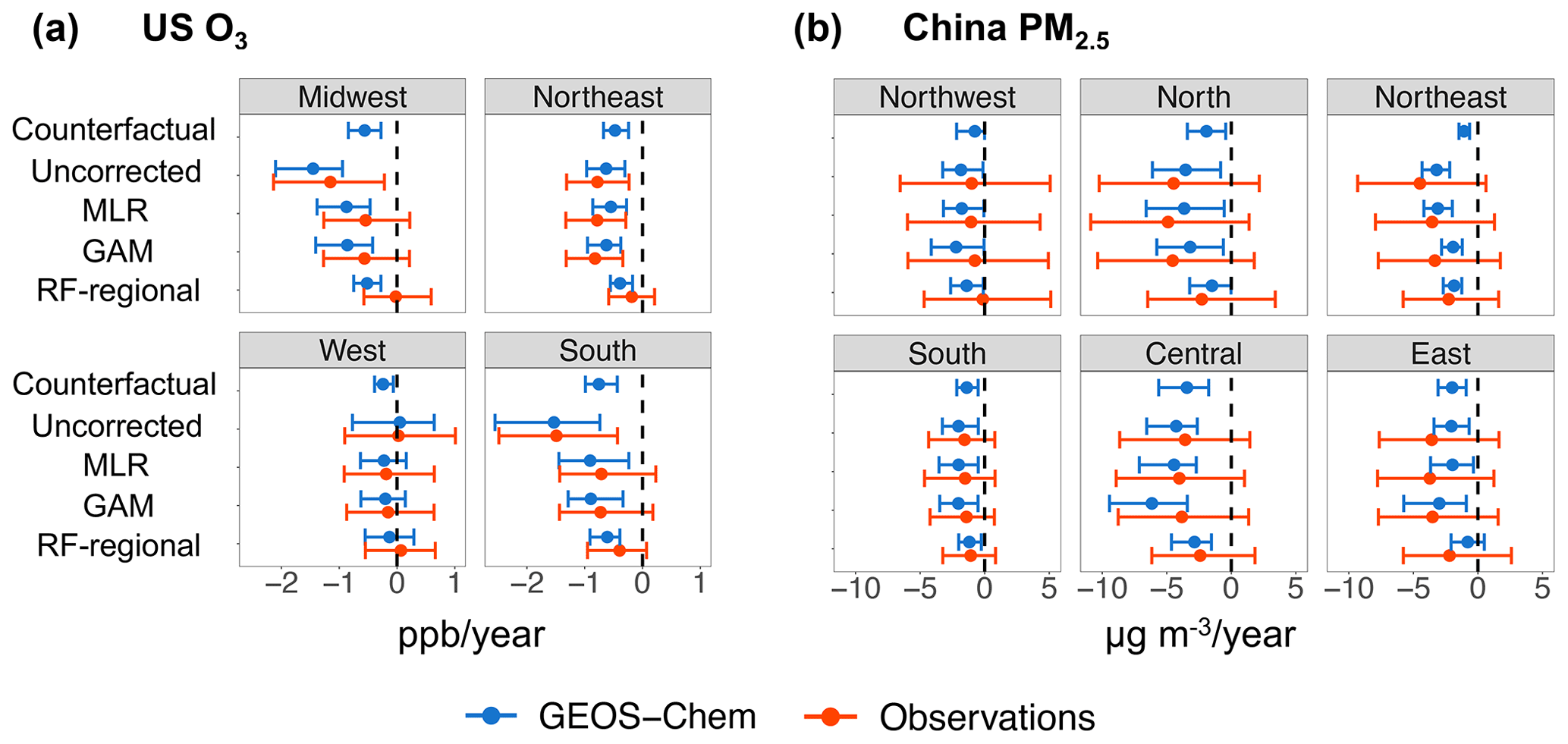
Figure 5 Trends in O₃ in the US (a) and PM_2.5 in China (b) estimated from the observational data (red) and GEOS-Chem simulations (blue) under different correction methods. Trends in pollutant concentrations are estimated at the monitor level (for the observational data) or at the grid cell level (for GEOS-Chem simulations). The point indicates the average value of the assessed trends of all monitors (or grid cells) within a region. The error bars show the 10th and 90th percentile of the assessed trends of all monitors/grid cells within a region. Panel (a) illustrates the summer O₃ trends in the US (unit: ppb yr⁻¹). Panel (b) illustrates the annual PM_2.5 trends in China (unit: $\mathrm{\mu }\mathrm{g}{\mathrm{m}}^{-\mathrm{3}}{\mathrm{yr}}^{-\mathrm{1}}$). We classify the US states into four regions according to the US Census Bureau and classify China's provinces into six regions based on the structure of China's subnational electric grid. Observational data are derived from US Environmental Protection Agency (2021a) and China's Ministry of Ecology and Environment (2021).

3.4 Application to observational data

Figure 5 shows the regional trends in O₃ in the US and trends in PM_2.5 in China estimated from the observational data from surface monitoring networks and the GEOS-Chem simulations (only grid cells that overlap with monitor locations are shown here). Here, to correct for the meteorology variability in observational data, we implement the same set of statistical methods as shown in Table 1 but with different numerical coefficients directly derived from the observational data. When applying different meteorological correction methods to the observational data, our analysis reveals that the choice of methods for meteorological correction can yield very different results for certain regions. For example, the regional average uncorrected O₃ trend is −1.49 and −1.15 ppb yr⁻¹ in the Midwest and South US, respectively, which overestimates the reductions in concentrations attributable to anthropogenic-emission changes (Fig. 5a). Correcting for the meteorological variability with the MLR model yields a regional average trend of −0.54 ppb yr⁻¹ in the Midwest (a decrease by 53 % in magnitude relative to uncorrected trends) and −0.71 ppb yr⁻¹ in the South US (a decrease by 52 %). RF-regional model further reduces the absolute magnitude of the declines in O₃ attributable to emission reductions to −0.02 ppb yr⁻¹ for the Midwest and −0.40 ppb yr⁻¹ for the South US. Importantly, these patterns are consistent with the results from our model experiments in these regions: the RF-regional model also estimates a much less negative emission-driven trend in the South US compared to the uncorrected case and MLR estimates in the GEOS-Chem simulations. For the GEOS-Chem simulations, RF-regional estimates are 39 % smaller than MLR estimates, and this is comparable to the magnitude changes for the observational data (RF-regional estimates are 44 % smaller than MLR). As the RF-regional model outperforms the other correction methods in recovering counterfactual trends in the GEOS-Chem simulations, this potentially also suggests a better performance of RF-regional in recovering the underlying emission-driven trends when applying to the observational data.

We find similar consistency in the method performances between observational data and GEOS-Chem simulations in China as well (Fig. 5b). When applying to the observational data from the surface monitoring network, a much smaller reduction in PM_2.5 concentrations is attributed to anthropogenic-emission changes in North, Northeast and East China using the RF-regional model, relative to the MLR estimates. For example, the average emission-driven trend estimated from the observational data is −4.9 $\mathrm{\mu }\mathrm{g}{\mathrm{m}}^{-\mathrm{3}}{\mathrm{yr}}^{-\mathrm{1}}$ in Beijing under the RF-regional model, compared with −9.6 $\mathrm{\mu }\mathrm{g}{\mathrm{m}}^{-\mathrm{3}}{\mathrm{yr}}^{-\mathrm{1}}$ under the MLR model. These patterns are consistent with the patterns of the trend estimates estimated from our GEOS-Chem simulations with different statistical methods.

4 Discussion

We designed a model experiment that enables us to directly quantify the performance of different statistical models to evaluate the trends in pollutant concentrations driven by anthropogenic-emission changes. Based on our evaluations of either PM_2.5 or O₃ trends across the US and China during periods of recent emission declines, our analysis shows that widely used MLR and GAM methods do not perform well in correcting for the meteorological variability and recovering simulated emission-driven trends. We propose a random forest model that uses both local and regional meteorological features, which offers the best overall performance in recovering the emission-driven trends across both species and countries. Applying this model to observational data suggests that estimates based on MLR or similar methods may overestimate the impacts of anthropogenic-emission changes on the decline in pollutant concentrations in certain regions in the US and China. However, the RF-regional method does not outperform all the other approaches in every location despite its better overall performance (see Figs. S14 and S15). This suggests that using multiple statistical approaches may be necessary to derive robust conclusions for attributing pollutant trends to emission changes.

With our model experiments, we also quantify the estimation errors in assuming emission impacts can be perfectly separated from meteorological variability. These errors likely bound the estimation errors that can be achieved by any statistical methods with this assumption. In the future, more complex statistical and machine learning methods could be applied to distinguish emission-driven and meteorologically driven changes, but attribution solely based on observed concentrations and meteorology will be limited by physical interactions between emissions and meteorology. We find that the estimation errors resulting from these interactions are overall much smaller compared to the estimation errors in the existing statistical methods but can still be important for certain regions at certain times. However, the intertwined relationships between anthropogenic emissions and meteorology are often much more complex in reality compared to our model experiments. For example, meteorology can also directly influence anthropogenic emissions (e.g., increased electricity consumption during extreme weather conditions, US Energy Information Agency, 2019; He et al., 2020). Therefore, the estimation errors that can be achieved by more flexible statistical models can potentially be even larger than the errors quantified with our constant-emis approach.

While the GEOS-Chem model provides us with a framework to test statistical methods, its use in our model experiments introduces some uncertainty and limitations. Specifically, our experiments assess the performance of statistical methods in correcting for the meteorology–pollution relationships encoded in GEOS-Chem, which may differ from the complex relationships in the observational data. Several studies have shown that GEOS-Chem and similar models do not capture certain meteorology–pollution relationships in the observational data (e.g., temperature–O₃ relationship, Porter and Heald, 2019, and influence of regional meteorological patterns, Fiore et al., 2009). The relationships encoded in GEOS-Chem may be different from the underlying meteorology–pollution relationships in the following three ways: (1) parameters in GEOS-Chem that describe these relationships are uncertain; (2) the relationships in GEOS-Chem are incorrect or incomplete; and (3) the relationships in GEOS-Chem are deterministic compared to the potential stochastic underlying processes. Therefore, the performance of any individual statistical method is likely to be worse in the real world compared to its ability to reproduce a deterministic meteorology–pollution relationship encoded in GEOS-Chem. Further model-based experiments could apply our methods to different atmospheric models in order to test if these conclusions differ by different models.

Changes in natural emissions due to meteorological variability play an important role in the air quality–meteorology relationship. Our model experiment considers natural emission changes that can be simulated online with assimilated meteorological fields in GEOS-Chem, including soil NO_x emissions, biogenic VOC emissions, and dust emissions. We find that the statistical models perform notably worse in correcting for the variability in dust-related PM_2.5 (see Fig. S12 for results using RF-regional), likely because dust PM_2.5 is extremely variable, with zero concentration on most non-dust days but extremely high concentration during the occasional dust storms. Our findings can potentially shed light on another important source of natural emissions, wildfire emissions, which are also quite variable but have become an increasingly important contributor to PM_2.5 and O₃ in certain regions (e.g., western US) (Burke et al., 2021). While emissions from biomass burning are held constant in our model experiments, as the wildfire emissions are prescribed in GEOS-Chem, wildfire emissions are significantly influenced by climatic variability (Abatzoglou and Williams, 2016; Xie et al., 2022) and will likely be a substantial challenge for any meteorological correction method in the future that attempts to separate changes in anthropogenic emissions from the variability in climate and associated natural emissions.

Our research reveals multiple directions for future research to enhance our understanding of the usage of statistical models to evaluate trends in pollutant concentrations under changing meteorological conditions. One key but challenging question is to better understand the estimation errors in these existing approaches; e.g., why the MLR model is able to correct for the meteorological variability in some locations but not others. In this paper, we only test a selection of methods based on their popularity in the existing literature and propose a simple-to-use model (RF-regional). More complex models (such as convolutional neural networks) may offer better performance, but the estimation error will likely be bounded by the errors in the constant-emis approach. Our work only evaluates the statistical and machine learning models in Eqs. (1) and (2), which only represent one (popular) set of evaluations that performs location-specific trend estimation with adjustments for meteorology and secular trends. However, other statistical model specifications specifically targeted to questions of meteorological interaction or that permit borrowing information across locations may generate different results. Constrained by computational resources and the availability of emission inventories, our simulation only covers a relatively short time period which could result in additional uncertainty in the linear trend estimates. When possible, future studies could evaluate performances of the statistical models with longer simulations and alternative trend estimates (such as the Theil–Sen estimator). A deeper investigation of the estimation error due to assuming perfect separation between meteorology and emission is also essential for understanding how we should interpret studies that use these statistical methods. For example, further work could explore how these errors will vary by the magnitude of emission reductions and the chemistry regimes.

5 Recommendations for attributing trends to emission changes

Using statistical methods to causally infer relationships between simulated air pollutant concentrations and anthropogenic emissions is challenging, and doing so in contexts of observational data is even more challenging. Understanding the uncertainty in statistical models in characterizing the meteorology–pollution relationship is essential to evaluating the effectiveness of policy interventions with observational data. Here, we make several recommendations to researchers and policymakers based on our analysis.

For those who aim to infer causal effects of emission changes on air quality based on observational data on concentrations and meteorology, we recommend using multiple statistical methods to correct for meteorological variability when evaluating the impacts of policies or interventions on air quality. From our two case studies, we find a relatively large variation between the trend parameters estimated by different statistical methods (especially at the grid cell or monitor level). Some methods perform better in certain locations but not in others (though RF-regional is the best-performing method overall). Using multiple approaches (linear/non-linear and at the local/regional scale) may help to quantify uncertainty related to meteorological corrections. These findings also suggest that empirical analyses may benefit from considering the impacts of meteorological variability on air quality separately for each region or even for each monitor location (if data permit), instead of attempting to determine a general relationship between meteorological variability and air pollution over a large spatial domain. Finally, analysts should be particularly cautious when using statistical methods to estimate impacts of anthropogenic emissions on air quality in regions where pollution variability is dominated by meteorologically influenced environmental processes such as dust emissions, as we consistently show that typical statistical methods (in combination with the standard set of meteorological variables) do not work well in those regions.

Due to the non-negligible estimation errors in recovering the counterfactual trends even with the best-performing statistical approach we test, we believe these statistical analyses are most useful in understanding the patterns of anthropogenic emissions on air quality when aggregated across larger spatial areas, rather than providing specific trends for individual monitor locations. There is a higher degree of consistency among the trend estimates across different methods when aggregated at regional level, but assessment at the local level is more sensitive to method choice. The absolute magnitude of monitor-level trends needs to be interpreted with caution, considering both the uncertainty from the statistical methods and also the limit of meteorological correction due to ignoring the interactions between meteorology and emissions.

Because measured pollutant concentrations are subject to the influence of underlying meteorological variability, many efforts have attempted to correct for the impacts of meteorological variability and use “meteorology-corrected” concentrations and trends to assist in evaluating the effectiveness of air quality policies. Our study evaluates existing methods that aim to correct for the meteorological variability and finds many of these methods do not perform well. This raises potential concerns about the use of meteorology-corrected concentrations as targets for policy evaluation. Meteorology-corrected concentrations and trends remain useful metrics to quantify the influence of emissions. However, a more comprehensive evaluation of the effectiveness of policy requires interpreting measurements with all available tools, ideally including both statistical analyses and physical models.