Weakening of tropical sea breeze convective systems through interactions of aerosol, radiation, and soil moisture

This study investigates how the enhanced loading of microphysically and radiatively active aerosol particles impacts tropical sea breeze convective systems and whether these impacts are modulated by the many environments that support these cloud systems. Comparisons of two 130-member pristine and polluted ensembles demonstrate that aerosol direct effects reduce the surface incoming shortwave radiation and the surface outgoing longwave radiation. Changes in the ensemble median values of the surface latent heat flux, the mixed layer depth, the mixed layer convective available potential energy, the maximum inland sea breeze extent, and the sea breeze frontal lift suggest that enhanced aerosol loading generally creates a less favorable environment for sea breeze convective systems. However, the sign and magnitude of these aerosol-induced changes are occasionally modulated by the surface, wind, and low-level thermodynamic conditions. As reduced surface fluxes and instability inhibit the convective boundary layer development, updraft velocities of the daytime cumulus convection developing ahead of the sea breeze front are robustly reduced in polluted environments across the environments tested. Statistical emulators and variance-based sensitivity analyses reveal that the soil saturation fraction is the most important environmental factor contributing to the updraft velocity variance of this daytime cumulus convection, but that it becomes a less important contributor with enhanced aerosol loading. It is also demonstrated that increased aerosol loading generally results in a weakening of the sea-breeze-initiated convection. This suppression is particularly robust when the sea-breeze-initiated convection is shallower and, hence, restricted to warm rain processes. While the less favorable convective environment arising from aerosol direct effects also restricts the development of sea-breeze-initiated deep convection in some cases, the response does appear to be environmentally modulated, with some cases producing stronger convective updrafts in more polluted environments. Sea breeze precipitation is ubiquitously suppressed with enhanced aerosol loading across all of the environments tested; however, the magnitude of this suppression remains a function of the initial environment. Altogether, our results highlight the importance of evaluating both direct and indirect aerosol effects on convective systems under the wide range of convective environments.

1 Introduction

Sea breeze convective systems are one of the key contributors to coastal cloudiness and rainfall in the tropics (Keenan and Carbone, 2008; Qian, 2008; Giangrande et al., 2014; Wang and Sobel, 2017). Differential heating over the land and ocean induces thermally driven baroclinic circulations, which modulate coastal air temperatures, impact coastal relative humidities, and redistribute coastal aerosols (Miller et al., 2003). Given their importance, a number of efforts have been made to examine how different atmospheric or land surface parameters modify tropical sea breeze convective systems (Qian et al., 2012; Grant and van den Heever, 2014; Bergemann and Jakob, 2016; Igel et al., 2018; Park et al., 2020b) and to improve their representation in numerical weather models (Boyle and Klein, 2010; Bergemann et al., 2017; Brown et al., 2017). However, in spite of these past studies, accurately predicting sea breeze convective systems remains challenging (Kidd et al., 2013; Azorin-Molina et al., 2014; Chen et al., 2015; Banta et al., 2020; Short, 2020). This is due in part to the large number of environmental parameters that impact the sea breeze convective system and in part to the fact that these parameters coexist, covary, and interact with one another (Crosman and Horel, 2010), which requires the use of sophisticated statistical approaches to identify those parameters predominantly responsible for sea breeze convection (Igel et al., 2018; Park et al., 2020b). Moreover, in association with the continuous increase in coastal human populations, a rise in aerosol emissions due to anthropogenic activities and biomass burning in the tropics has been observed (Reid et al., 2012; Wang et al., 2013; Menut et al., 2018). The presence of aerosols can further complicate the behavior of sea breeze convective systems through radiative, microphysical, and dynamical feedback processes. Aerosol emissions and processes may also, in turn, be modulated by the environmental parameters. While the basic processes driving sea breeze convective systems are relatively well understood, the impacts of aerosols on sea breeze convective systems, and the modulation of these impacts by various environmental properties, have not received much attention.

Aerosol particles can interact directly with shortwave and longwave radiation through scattering and absorption (McCormick and Ludwig, 1967; Charlson and Pilat, 1969; Atwater, 1970; Mitchell, 1971; Coakley et al., 1983). These aerosol direct effects have numerous implications for processes important to the development of shallow and deep convection. Scattering and absorption of shortwave and longwave radiation, and the subsequent reemission of longwave radiation at the surface, influence surface sensible and latent heat fluxes and near-surface temperatures, all of which impact the development of the convective boundary layer. A number of studies have highlighted the importance of considering both the radiative and microphysical effects of aerosol particles on convective boundary layers and inversions. For example, within an aerosol–radiation–land surface feedback framework, reduced surface sensible heat fluxes due to aerosol direct effects have been found to stabilize the lower troposphere, suppress boundary layer development and convective available potential energy (CAPE), and enhance the capping inversion (Yu et al., 2002). As a result, shallow convection and precipitation over land have been found to become weaker (Jiang and Feingold, 2006; Niyogi et al., 2007). From these studies, it is clear that aerosol–radiation interactions may have important feedbacks to the environment and the resulting sea breeze convective system. Nevertheless, studies of aerosol impacts on cloud properties, in particular deep convection, have quite often neglected aerosol–radiation interactions (e.g., Storer and van den Heever, 2013; Miltenberger et al., 2018; Marinescu et al., 2021).

Depending on their sizes and compositions, various aerosol particles can serve as cloud condensation nuclei (CCN). Under the assumption of the same liquid water content, when the number concentration of CCN is increased, a greater number of smaller cloud droplets are formed, thereby increasing the cloud albedo (Twomey, 1974) and the cloud lifetime (Albrecht, 1989), in what are often referred to as the first and second aerosol indirect effects, respectively. Less efficient collision and coalescence processes between the population of more numerous smaller cloud droplets suppresses the warm rain process, resulting in the longer cloud lifetimes described in the second indirect effect. These aerosol effects were initially postulated for shallow convective clouds but have also been observed to occur in deep convective cloud systems (Tao et al., 2012). It has been further hypothesized that, with the suppression of the warm rain process, more numerous cloud droplets are lifted above the freezing level and frozen, thereby releasing additional latent heating and potentially strengthening updrafts. This process, which takes place in the mixed- and cold-phase regions of clouds, is often referred to as the cold-phase invigoration and has been reported in both observational and modeling studies (e.g., Andreae et al., 2004; Khain et al., 2005; Koren et al., 2005; van den Heever et al., 2006; Rosenfeld et al., 2008). Under increased aerosol loading, the condensational growth rate of the population of more numerous smaller cloud droplets within the warm phase regions of deep convective clouds has also been observed to increase due to the greater exposed total droplet surface area, thereby releasing more latent heating and enhancing convective updrafts closer to cloud base. These warm-phase aerosol–cloud dynamical feedbacks have collectively been termed condensational invigoration (Kogan and Martin, 1994; Seiki and Nakajima, 2014; Saleeby et al., 2015; Sheffield et al., 2015) or warm-phase invigoration (Fan et al., 2018). It has recently been suggested that warm-phase invigoration may be more significant and robust than its cold-phase counterpart (Grabowski and Morrison, 2016, 2020; Marinescu et al., 2021; Igel and van den Heever, 2021).

While convective invigoration hypotheses have proposed stronger updrafts and/or heavier precipitation for convective clouds developing within enhanced aerosol loading conditions, a number of studies have questioned the robustness of these hypotheses for various reasons (Grabowski and Morrison 2016, 2020), one of which is the modulation of these effects by the cloud environment. For example, wind shear (Fan et al., 2009; Lebo and Morrison, 2014; Marinescu et al., 2017), CAPE (Lee et al., 2008; Storer et al., 2010, 2014), boundary layer instability (Marinescu et al., 2021), moisture (Khain et al., 2005, 2008; Tao et al., 2007; Grant and van den Heever, 2015), and aerosol–meteorology covariation (Varble, 2018) have all been found to modulate aerosol impacts on cloud systems. Such environmental modulation has not been explored in the context of sea breeze convective systems in spite of the fact that they are one of the most ubiquitous forms of convection in the tropics (Hadi et al., 2002; Perez and Silva Dias, 2017) and, as such, form the focus of this paper. The primary goals of this study are twofold. The first goal is to investigate how radiatively and microphysically active aerosols change the convection that develops within tropical sea breeze regimes, specifically over land. The second goal is to determine whether and how these convective responses to enhanced aerosol loading are modulated by the large number of environmental factors supporting sea breeze convective systems.

2 Methods

2.1 RAMS model configuration

There are two large ensembles of idealized numerical simulations of tropical sea breezes conducted using the Regional Atmospheric Modeling (RAMS) version 6.2.08 (Cotton et al., 2003; Saleeby and van den Heever, 2013). Idealized simulations are useful in that they are sufficiently complex to capture the storm systems of interest but are also sufficiently simple to allow for the isolation and evaluation of the critical physical processes at play, without the addition of unnecessary confounding factors often present in more complex case study simulations. As our focus is on tropical sea breeze convection, the idealized simulations are initialized using conditions that are representative of equatorial coastal rainforest regions, more specifically, the Cameroon rainforest region (Grant and van den Heever, 2014).

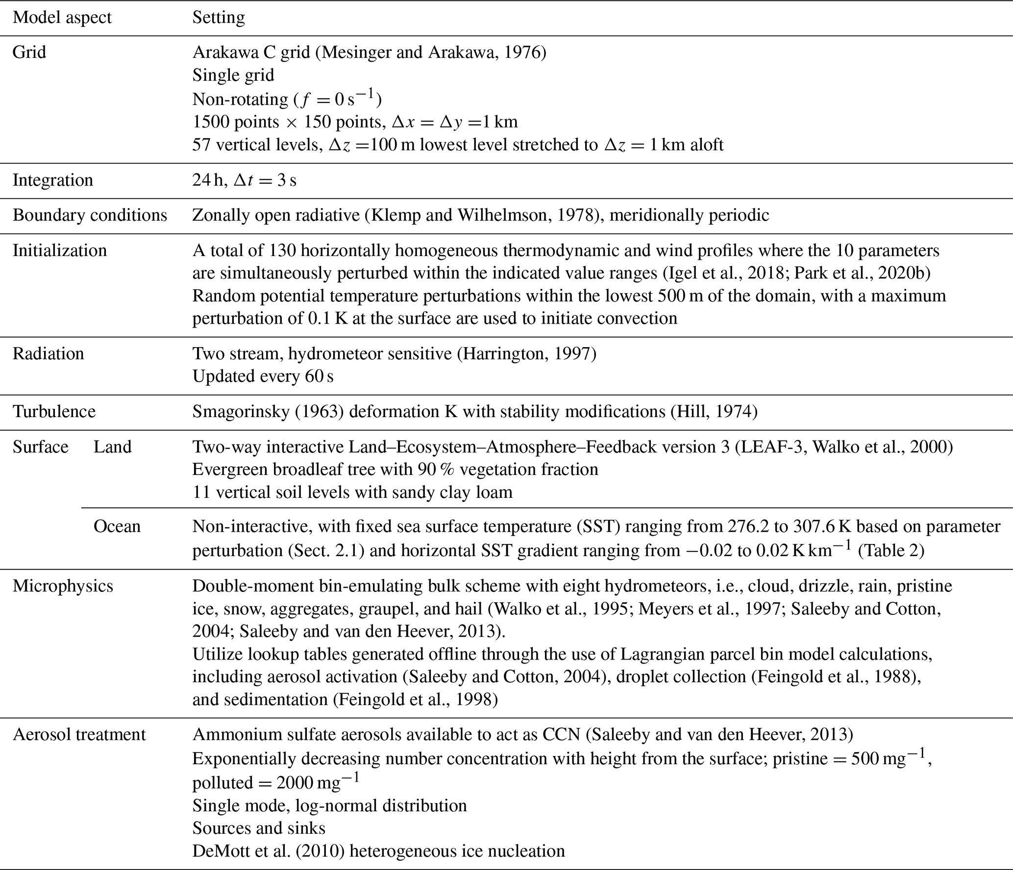
The RAMS model configuration used here is identical to that used in Park et al. (2020b). The boundary conditions, initialization, and physical schemes are summarized in Table 1. The horizontal grid spacing is 1 km, and a 100 m vertical grid spacing near the surface is vertically stretched to 1 km near the model top. Each simulation is run from 00:00 local time (LT) for 24 h using a 3 s time step. Output files are saved every 10 min. RAMS is coupled to the Land–Ecosystem–Atmosphere Feedback version 3 (LEAF-3), a fully interactive soil–vegetation–atmosphere parameterization (Lee, 1992; Walko et al., 2000). To simulate an idealized sea breeze circulation, two different surfaces, one land and one ocean, are separated by a straight coastline located at the center of the domain. In our idealized setup, the western half of the domain represents the land region and is specified to be a rainforest with evergreen broadleaf trees and sandy clay loam soil type, following that of Grant and van den Heever (2014). The eastern half of the domain is over ocean, and the sea surface temperature and horizontal gradient are kept fixed throughout the simulation. These relative locations of land and ocean are chosen arbitrarily and could have just as easily been the other way around.

Table 1 The RAMS model configuration used to conduct the pristine and polluted ensembles.

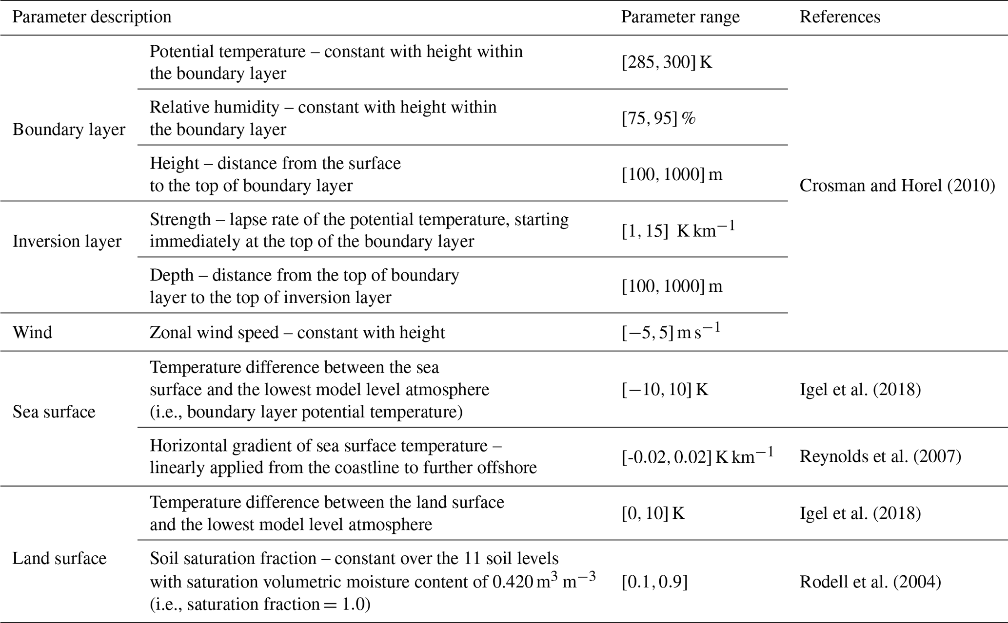
All of the simulations are initialized with horizontally homogeneous thermodynamic and wind profiles. As described in Park et al. (2020b), we make use of 130 different initial environmental conditions, where 10 different lower tropospheric thermodynamic, wind, and surface properties (Table 2) are simultaneously perturbed across a range of values representative of tropical equatorial regions. The range in the selected variables were sourced from the sea breeze literature, the reasons for which were described in detail in Igel et al. (2018). While statistical distributions of the parameters of interest are very difficult to find in the literature, plausible parameter ranges for tropical regions were assigned to each of the variables tested. Should new observations provide greater constraints on the range of these parameters, the emulator approach (described below) allows for an assessment of the responses of the sea breeze convective system to the range of parameter values of interest. The 10 selected parameters are perturbed using maximin Latin hypercube sampling (Morris and Mitchell, 1995), a space-filling algorithm, to ensure optimal coverage of the 10-dimensional parameter space with a minimum number of parameter combinations, and hence, it determines the minimum number of simulations that need to be conducted. As shown in Park et al. (2020b), this amounts to 130 simulations in each of the ensembles conducted here. It should be emphasized that these 130 different initial conditions represent more than 59 049 (=3¹⁰) different initial conditions had only three values for each of the 10 parameters been selected. For the lower tropospheric thermodynamic properties, the following five parameters defining the structure of the boundary layer and inversion layer are considered based on their potential influences on instability and the moisture available for moist convective development: (1) the boundary layer potential temperature, (2) the boundary layer relative humidity, (3) the boundary layer height, (4) the inversion layer depth, and (5) the inversion layer strength. The upper tropospheric thermodynamic profiles above the inversion layer are identical for all 130 initial conditions and utilize the initial sounding of Grant and van den Heever (2014). The initial zonal wind speed, which has been extensively studied regarding its control on the inland propagation speed and extent of the sea breeze (Crosman and Horel, 2010), is also considered and represents the sixth environmental factor examined. It should be noted that the initial zonal wind speed contains no vertical wind shear, although this does develop as the simulations progress. Finally, sensitivity to the variations in the surface characteristics are also examined considering their potential impact on surface moisture and turbulent fluxes, including (7) the soil saturation fraction, (8, 9) the temperature difference between land/ocean surface and the atmospheric temperature at the lowest model level, and (10) the horizontal gradient of sea surface temperature (SST). Additional details, and the range of each of these parameters utilized in these ensembles, are shown in Table 2.

Table 2 The 10 environmental parameters perturbed in this study and their uncertainty range.

For the sake of simplicity, the aerosol type utilized in this study is restricted to single-mode, submicron ammonium sulfate. We chose ammonium sulfate due to its ubiquity in the atmosphere and its ability to serve as CCN as a result of its high solubility. While the aerosol field is initialized horizontally and homogeneously using appropriate profiles of aerosol (as discussed below), aerosol particles are allowed to be redistributed via advection, convection, and nucleation following initialization. Aerosol sources and sinks, including the return of aerosols to the environment following evaporation, are all also incorporated (Saleeby and van den Heever, 2013).

2.2 Experimental setup

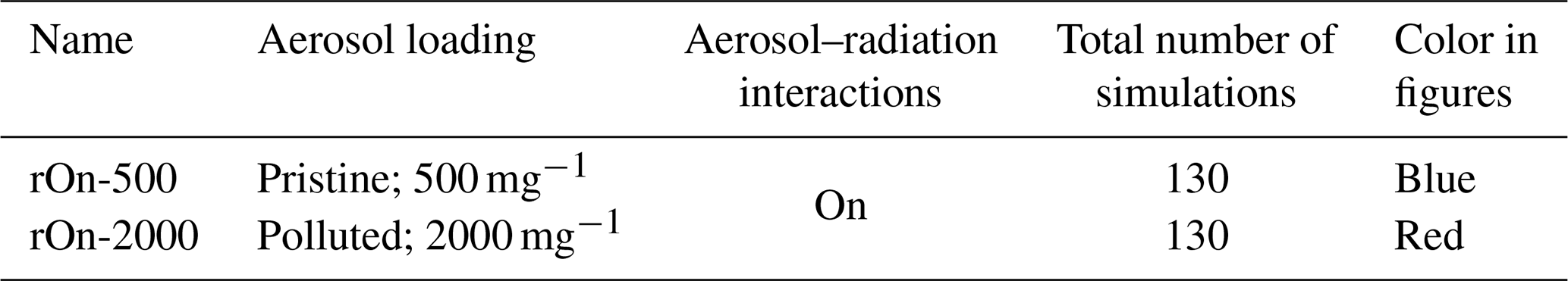
There are two different ensembles of idealized simulations with different aerosol concentrations performed for this analysis. The nomenclature and description of each of the ensembles are summarized in Table 3. Here, “r” refers to aerosol–radiation interactions, and “On” means that aerosol particles are allowed to interact with radiation. It should be noted that radiation is always fully interactive with both aerosols and hydrometeor species in both of the ensembles analyzed here. We have conducted additional ensembles in which we have turned the aerosol–radiation interactions off to investigate the impacts on the deep convective mode, the results of which will be published elsewhere. The rOn-500 ensemble is the suite of simulations examined in Park et al. (2020b) in which the model is initialized with surface aerosol concentrations of 500 mg⁻¹ (blue line) and which decrease exponentially with height, as shown in Fig. 1. To examine the impacts of increasing the aerosol loading on sea breeze convection, this ensemble of simulations is repeated, but with aerosol concentrations of 2000 mg⁻¹ (red line in Fig. 1) at the surface, and again using an exponentially decreasing profile. This model ensemble is referred to as rOn-2000. The surface aerosol concentrations are chosen based on observations made in equatorial Africa (Andreae et al., 1992; Kacarab et al., 2020). The exponentially decreasing initial profiles are used in the interests of simplicity, and they soon evolve as a result of the processes described above. We shall use the terms “pristine” and “rOn-500” interchangeably and “polluted” and “rOn-2000” interchangeably throughout this work. It is important to note that, while 130 different initial conditions are implemented in each ensemble, the polluted and pristine ensembles utilize the same 130 different initial conditions, thereby facilitating direct comparison between the corresponding pristine and polluted ensemble pairs. Also, as the 130 initial environmental conditions represent the 10-dimensional input parameter space, these pristine and polluted ensembles allow us to evaluate the ways in which direct and indirect aerosol impacts on sea breeze convection are modulated by the large number of different environments supporting the development of such sea breeze regimes.

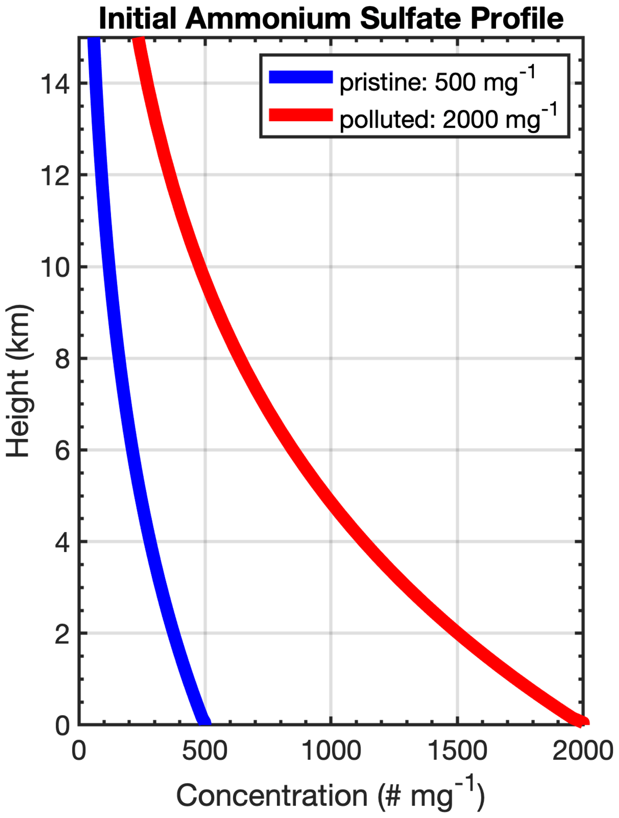
Figure 1 Initial number concentration of ammonium sulfate for the pristine (blue line; 500 mg⁻¹ at the surface; rOn-500) and polluted (red line; 2000 mg⁻¹ at the surface; rOn-2000) model ensembles.

Table 3 The naming convention and descriptions of the two model ensembles conducted for this research.

2.3 Analysis methodology

In a manner similar to Park et al. (2020b), we apply an advanced statistical algorithm developed by Lee et al. (2011) and Johnson et al. (2015) that includes statistical emulation (O'Hagan, 2006) and a variance-based sensitivity analysis (Saltelli et al., 1999) over the 10-dimensional input parameter space. Due to its computational efficiency, this advanced statistical algorithm has been successfully utilized in several modeling studies that quantify the sensitivity of numerical model responses to a range of input parameters (Feingold et al., 2016; Igel et al., 2018; Wellmann et al., 2018, 2020; Glassmeier et al., 2019; Marshall et al., 2019; Park et al., 2020b). This algorithm incorporates the Gaussian process emulation (O'Hagan, 2006; Rasmussen and Williams, 2006) to build a statistical surrogate representation of the complex cloud-resolving model responses of the parameters of interest. Over the 10-dimensional parameter space, the emulator estimates the cloud-resolving model responses of interest at untried input parameter combinations, thereby densely sampling the output of interest and thus allowing us to understand the relationship between the perturbed input parameter and output responses without having to conduct the simulations representative of each set of perturbed parameters. We can then quantify the relative importance of the perturbed input parameters on the output of interest via variance-based sensitivity analyses. Further details of how this approach is used to determine the predominant environmental factors impacting tropical sea breeze convective systems are included in Park et al. (2020b). We now begin our analysis by examining the morphology of the convection that develops within the pristine and polluted ensemble of simulations.

3 Basic description of the sea breeze simulations

In this section, an overview of the convective morphology and development within our tropical sea breeze simulations is provided. A sea breeze circulation develops after sunrise (06:00 LT), and convergence along the leading edge of the sea breeze front becomes evident at the coastline, where the highest land–sea thermal contrast is established (not shown). Throughout the daytime hours, and even shortly after sunset (18:00 LT), the sea breeze front continues to propagate further inland, which is in keeping with the classical theory of such baroclinic circulations. The sea breeze front is observed to develop in all 260 simulations comprising the rOn-500 and rOn-2000 ensembles (130 simulations in each ensemble), the location of which is detected at every output time step, using an identification algorithm developed by Igel et al. (2018).

There are two types of convection evident over land between 12:00 and 18:00 LT (Fig. 2), as is often the case with tropical sea breeze systems. Ahead of the leading edge of the sea breeze, daytime heating and mixing induce cumulus convection, whereas along the leading edge of the sea breeze front, where low-level air parcels may be lifted to the level of free convection through low-level convergence, sea-breeze-initiated deep convection may occur. As shown in Park et al. (2020b), the strength of the sea breeze circulation and the associated convergence along the leading edge vary strongly as a function of the initial environmental conditions. Such variations result in a range of shallow through deep convective clouds being produced in association with the sea breeze front. The left column of Fig. 2 displays one example from the rOn-2000 ensemble, where both the daytime cumulus convection ahead of the sea breeze and the convection developing along the sea breeze front are shallow (cloud top heights <4 km a.g.l. – above ground level) and remain so throughout the simulation. While both types of convection remain shallow in this scenario, the sea-breeze-initiated convection is characterized by deeper clouds and stronger updrafts than the daytime cumulus convection forming ahead of this line. In the right column of Fig. 2, the development of deep convection (cloud top heights >7 km a.g.l.) along the sea breeze front in another ensemble member is shown. In this case, the convection initiated by the sea breeze is significantly deeper than the previous case, and this sea-breeze-initiated deep mode is accompanied by significantly heavier precipitation and stronger updrafts than those associated with the sea-breeze-initiated shallow modes. The vast majority of the ensemble members fall into the shallow mode scenario, whereas only a handful of the ensemble members display deep-mode convection. Throughout the rest of the paper, we will refer to the convection developing out ahead of the sea breeze front as “daytime cumulus convection” and to the convection developing along the sea breeze front as the “sea-breeze-initiated convection”. The terms “shallow mode” and “deep mode” will be used to distinguish the different types of sea-breeze-initiated convection.

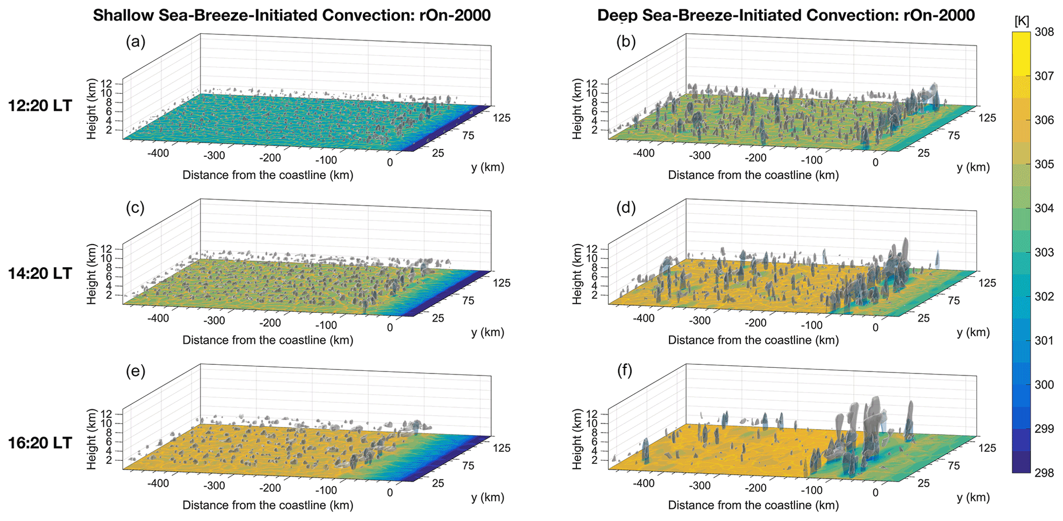
Figure 2 Examples of the convective morphologies observed in the rOn-2000 ensemble where the sea-breeze-initiated convection remains shallow throughout the domain (left column; Test 14; shallow mode) and in which deep convection develops along the sea breeze front (right column; Test 27; deep mode) at 12:20 (a, b), 14:20 (c, d), and 16:20 LT (e, f). Gray isosurfaces are where the total condensate, with the exception of rain, is 0.1 g kg⁻¹, and the dark blue isosurfaces are where the rain mixing ratio is 0.1 g kg⁻¹. The shaded contours at the surface represent the density potential temperature (K; Emanuel, 1994) at the lowest model level. Only a 520 km×130 km subset of the domain is displayed here.

4 Aerosol impacts on the convective environment

In order to examine the impacts of aerosols on the convective environment, we first examine the effects of varying aerosol concentrations on the surface radiation budget. As ammonium sulfate aerosols are allowed to scatter and absorb radiation as a function of the wavelength, median radius, and relative humidity within RAMS (Saleeby and van den Heever, 2013), less incoming solar radiation is expected to reach the surface. These aerosol direct effects are addressed by analyzing the differences in surface downwelling shortwave and surface upwelling longwave radiation between rOn-500 and rOn-2000 for clear-sky columns. To identify the clear-sky columns, the total condensate mixing ratio was required to be smaller than 0.01 g kg⁻¹ at all vertical levels within the column. As the aerosol number concentrations are increased between the pristine and polluted ensembles, the clear-sky downwelling shortwave radiation decreases throughout the atmosphere over land and ocean, with the maximum difference occurring at the surface for all 130 corresponding pairs of simulations of the rOn-500 and rOn-2000 ensembles (Fig. 3a and b). The daytime-averaged (06:00–18:00 LT) surface shortwave radiation difference between rOn-500 and rOn-2000 is 81.2 W m⁻² for the ensemble average and has a standard deviation of 6.5 W m⁻².

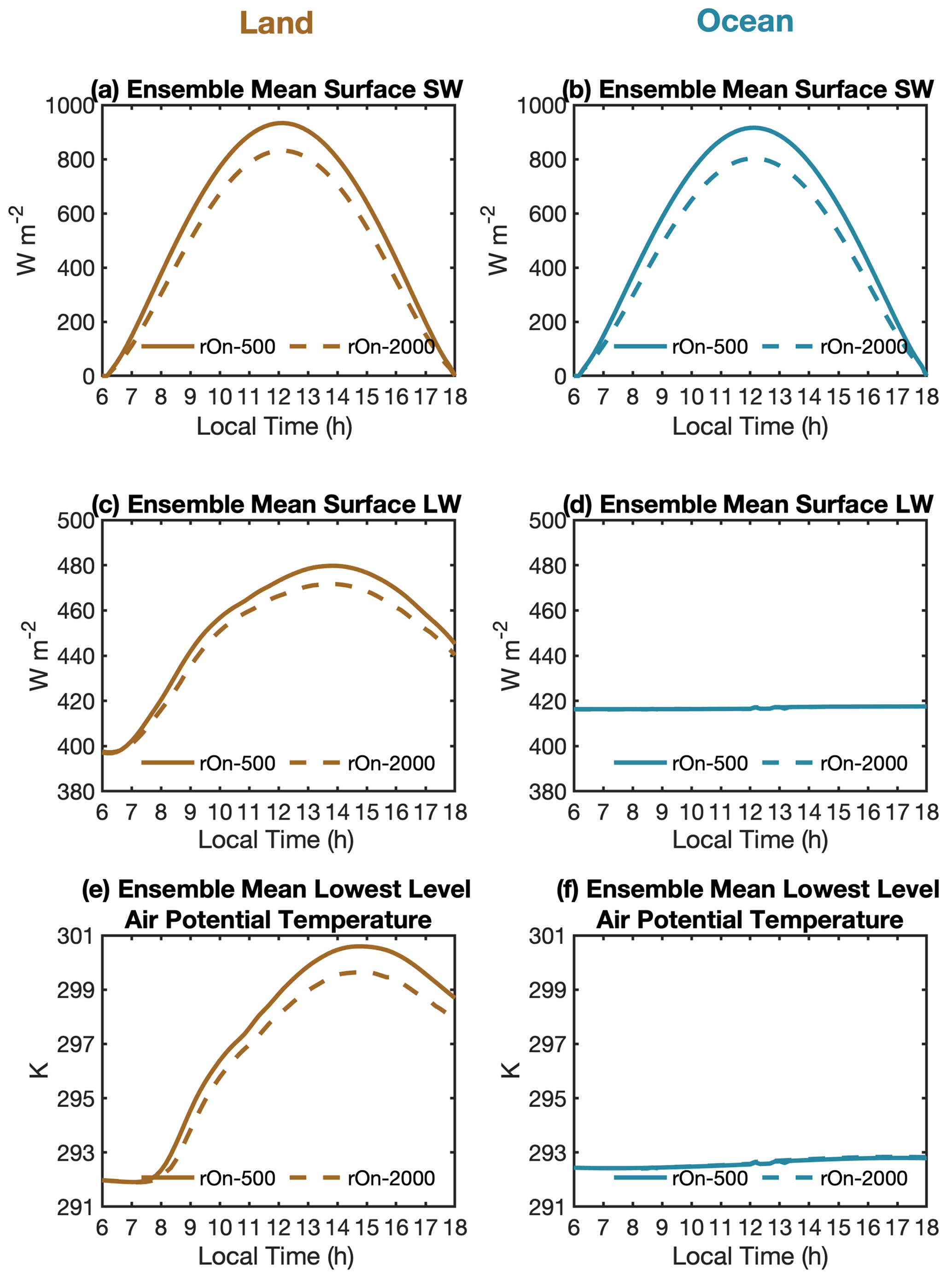
Figure 3 Time series of each ensemble mean (a, b) surface downwelling shortwave radiation, (c, d) surface upwelling longwave radiation, and (e, f) lowest model level potential temperature over land (left column; brown lines) and ocean (right column; blue lines). Solid and dashed lines denote rOn-500 and rOn-2000, respectively.

The surface upwelling longwave radiation (Fig. 3c and d) reflects the aerosol-induced changes in incoming solar radiation. Due to the much lower heat capacity of the land surface compared to the ocean surface, the longwave emission significantly decreases over the interactive land surface as it rapidly responds to the reduction in shortwave radiation in the polluted ensemble. With less surface upwelling longwave radiation, the air above the land becomes cooler (Fig. 3e) for the conditions of enhanced aerosol loading compared to the more pristine conditions. Over the ocean regions, the SST is fixed throughout the duration of each ensemble member simulation, although it can be different between ensemble members based on the environmental parameter being perturbed. As such, the potential temperature of the lowest level of air does not change significantly over the ocean since the longwave radiation emitted from the surface remains almost the same (Fig. 3f). However, even if the SST had been allowed to be interactive, given the higher heat capacity of the ocean, the upwelling longwave radiation from the ocean surface would not respond as quickly to the aerosol-induced reduction in shortwave radiation as that over the land surface. As a result of these aerosol interactions with the radiation, the ensemble mean surface temperature difference between the ocean and the land is less in the polluted case when compared with the pristine case (Fig. 3e and f), which has important implications for the strength of the thermally driven sea breeze circulation. These are discussed in more detail below.

The aerosol-induced reduction in incoming solar radiation reaching the surface also impacts the surface fluxes. Figure 4 displays the temporal evolution of the surface sensible and latent heat fluxes of the environment ahead of the sea breeze front, averaged over all 130 simulations in each ensemble. Both the ensemble mean sensible and latent heat fluxes are reduced in rOn-2000 compared with rOn-500 as a result of the enhanced aerosol loading. The maximum aerosol-induced reduction is 45 % and 60 %, and the mean is 19 % and 15 %, for the sensible and latent heat fluxes, respectively. This reduction in incoming solar radiation and associated surface flux responses due to enhanced aerosol loading is in close agreement with the findings from previous studies (Yu et al., 2002; Koren et al., 2004; Feingold et al., 2005; Jiang and Feingold, 2006; Zhang et al., 2008; Grant and van den Heever, 2014). These reductions in sensible and latent heating will negatively impact the convective boundary layer by limiting both the heating and moistening of this layer. Specifically, less moisture will be available for the convection via evapotranspiration, evaporation, and condensation, which is reflected in the reduction of the ensemble median surface latent heat flux in the polluted case (Fig. 5a), as well as the differences between the polluted and pristine ensembles, the vast majority of which are negative (Fig. 5b). The surface-based mixed layer depth, defined here as the level above the surface at which the vertical gradient of the potential temperature first exceeds 2 K km⁻¹, decreases in rOn-2000 compared with rOn-500 due to this reduction in surface sensible heat flux and associated turbulent mixing. Histograms of the mean surface based-mixed layer depth ahead of the sea breeze front in rOn-500 and rOn-2000 and their differences are shown in Fig. 5c and d, respectively. In Fig. 5c, the mean mixed layer depth distribution shifts toward lower values with the change from rOn-500 to rOn-2000. This aerosol-induced decrease in mixed layer depth is also evident in the reduced ensemble median values (vertical lines in Fig. 5c) in rOn-2000 compared with rOn-500. Figure 5d further indicates that the mixed layer in each member of the rOn-2000 ensemble is shallower than the corresponding mixed layer in the rOn-500 ensemble, with all of the rOn-2000 minus and rOn-500 values being negative.

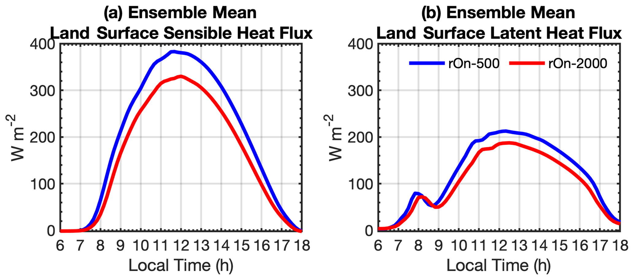
Figure 4 Time series of the ensemble mean land surface (a) sensible heat flux and (b) latent heat flux, spatially averaged from western domain edge to the 50 km ahead of the algorithm-identified sea breeze front, for the rOn-500 (blue) and rOn-2000 ensembles (red).

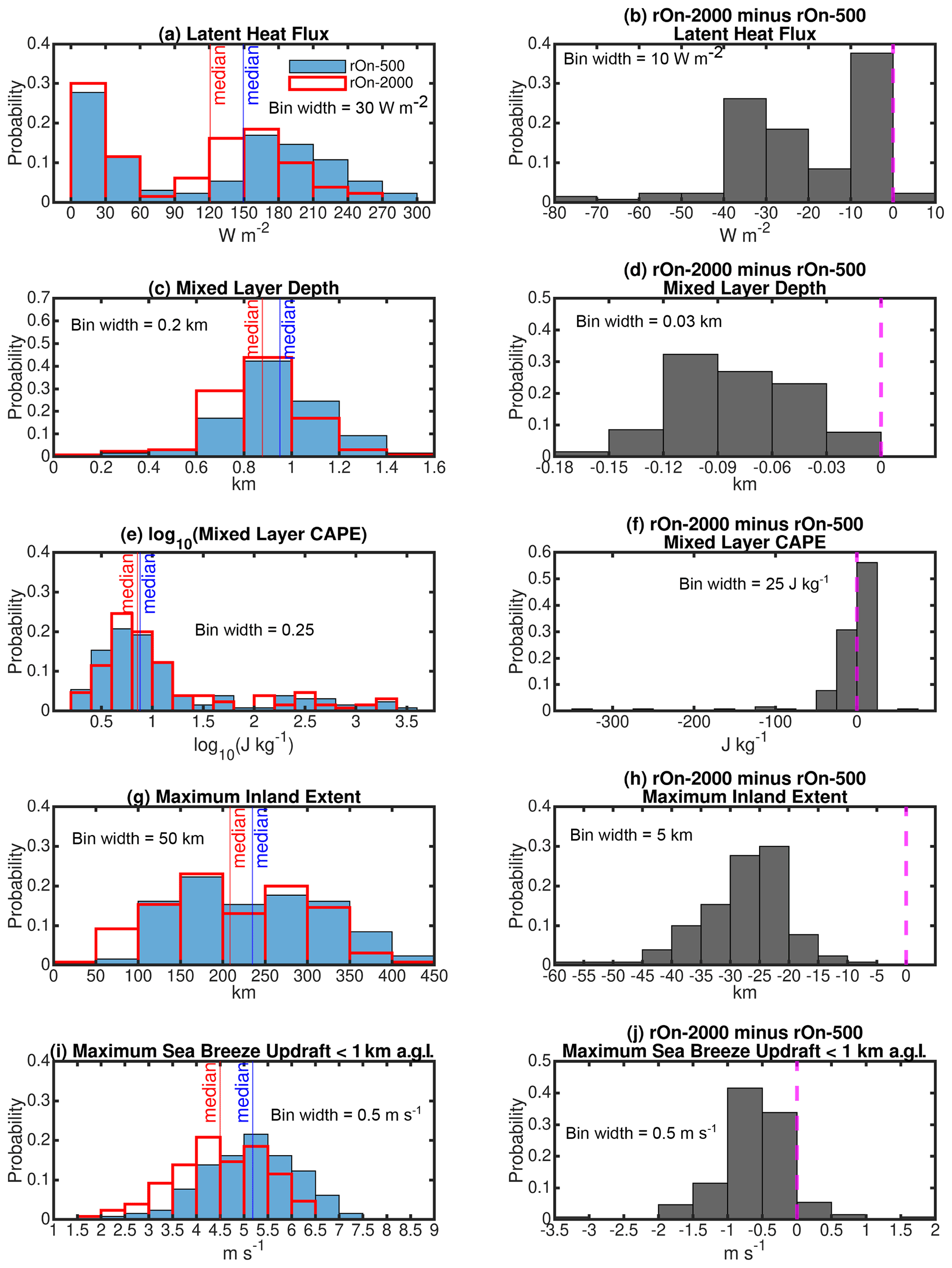
Figure 5 Histograms of (a) the land–surface latent heat flux (W m⁻²), (c) the surface-based mixed layer depth (km), and (e) the logarithm of the mixed-layer CAPE (J kg⁻¹), all of which are averaged for each ensemble from the western domain edge to 50 km ahead of the algorithm-identified sea breeze front between 12:00 and 18:00 LT. (g) The maximum inland extent of the sea breeze front (km) and (i) the maximum low-level (below 1 km a.g.l.) updraft velocities within ±1 km of the algorithm-identified sea breeze front (m s⁻¹) are shown. The median values of each characteristic are marked by the red and blue thin vertical lines. The light blue shading and the red lines represent rOn-500 and rOn-2000 ensembles, respectively. (b, d, f, h, j) Histograms of the differences in the corresponding fields shown in panels (a), (c), (e), (g), and (i) arising due to aerosol loading (rOn-2000 minus rOn-500). The dashed magenta lines indicate where the difference between rOn-2000 and rOn-500 is zero. The bin width of each histogram is marked in the upper corner of each panel.

While mixed layer depth is a valuable indicator of instability in the boundary layer and hence the depths of shallow cumulus, CAPE is a more pertinent assessment of instability for the deep convective clouds driven by the sea breeze convergence. As shown in Fig. 5e, most of the simulations in both ensembles have averaged mixed-layer CAPE values close to zero which is in keeping with the fact that only a handful of the simulations produce deep convection members. The ensemble median values are slightly reduced with enhanced aerosol loading, from 7.6 to 7.1 J kg⁻¹. The minimum CAPE values in rOn-500 and rOn-2000 are 1.8 and 2.0 J kg⁻¹. Figure 5f also demonstrates that the differences in CAPE between rOn-500 and rOn-2000 may be positive or negative but are mostly quite small in magnitude. The exceptions to this are the magnitudes and differences for those five cases that produce deep convection in rOn-500 but not in rOn-2000, where the CAPE values may be as high as 2086 J kg⁻¹, and the aerosol-induced differences are all negative and range in magnitude from 8 to 115 J kg⁻¹. Therefore, while the variations in CAPE with aerosol loading appear to be small in magnitude for most members of the ensembles, they may play a discriminating role in aerosol impacts on deep convective updraft velocities for those cases that do support deep convection. This is discussed further in Sect. 5.2.1.

We now turn our attention to the vertical lift provided by the convergence along the sea breeze front in all of the simulations. Classical sea breeze theory dictates that, to first order, the faster the sea breeze moves, the further inland the sea breeze travels during the day, the stronger the convergence along the sea breeze front, and hence the greater the vertical lift along the front. Here we examine the maximum inland extent of the sea breeze front and the maximum updraft velocity found within ±1 km of the algorithm identified surface location of sea breeze front during the afternoon (12:00–18:00 LT). The maximum inland extent of the sea breeze front is identified as the last inland location of the sea breeze front detected by the sea breeze front algorithm (Igel et al., 2018). We assess the low-level (below 1 km a.g.l.) maximum vertical velocity within ±1 km of the surface location of the objectively identified front in order to account for any forward bulging or backward tilting of the frontal boundary in relation to the identified location of the front at the surface and to ensure that the updrafts are primarily driven by the frontal convergence as opposed to the possibility of buoyant forcing. The distribution of the maximum sea breeze inland extent shows a shift towards lower values with enhanced aerosol loading (Fig. 5g), also evident in the decrease in the ensemble median with enhanced aerosol loading (Fig. 5g). It is also evident from Fig. 5h that the sea breeze extent is less in rOn-2000 than rOn-500 for each and every one of the ensemble pairs, thus demonstrating the significant role of aerosol loading and the direct effect on this baroclinic circulation and the subsequent forcing of deep convection. The distribution of the maximum updraft velocities (and hence lift) along the sea breeze front shows a shift towards reduced updraft velocities in more polluted environments, as is demonstrated by the small reduction in the ensemble median of rOn-2000 compared with rOn-500. However, in spite of the robust response of the maximum inland extent of the sea breeze to aerosol loading (Fig. 5h), the impacts of enhanced aerosol loading on the maximum frontal velocities do not always produce a negative vertical velocity response (Fig. 5j). This suggests that, while the environment does not appear to modulate the direct impacts of aerosols on the sea breeze dynamics and inland extent, it may locally modulate aerosol impacts on the updraft velocities, possibly through aerosol indirect processes and/or changes to CAPE.

Finally, a weaker aerosol-induced sea breeze circulation was also observed in Grant and van den Heever (2014). However, in that study, only one set of initial environmental conditions was utilized. One might therefore wonder whether such findings are applicable to the multiple other environments known to support sea breeze systems or whether various sea breeze environments produce a different response to aerosol loading. Since rOn-500 and rOn-2000 each have 130 different initial conditions, and as these initial conditions are representative of the wide range of environmental parameter values previously identified as being responsible for generating sea breeze systems, these results suggest that the aerosol-induced weakening of sea-breeze-initiated convection, at least through aerosol direct effects on the sea breeze circulation and extent, is indeed a relatively robust result and is one that appears to occur in the majority of sea breeze environments.

5 Impacts of enhanced aerosol loading on continental convection

Now we seek evidence of the impacts of increased aerosol number concentrations on the intensity of the convection within tropical sea breeze convective system as a result of both direct and indirect aerosol effects. More specifically, we investigate the impacts of enhanced aerosol loading on cloud top heights, convective updraft velocities, and precipitation, all of which are common indicators of convective intensity (e.g., Nesbitt and Zipser, 2003).

5.1 Cloud top heights

We examine the impacts of aerosol loading on cloud top height in two ways. First, we examine the frequency distribution of the fraction of low (cloud top height <4 km) cloudy columns to the total number of cloudy columns for all simulations (low cloud columns/all cloudy columns; Fig. 6a). Among the 130 simulations in each ensemble, there are 104 and 113 simulations with low clouds only in rOn-500 and rOn-2000, respectively. The vast majority of ensemble members in both ensembles is therefore dominated by low clouds, as demonstrated by the ensemble median values of 100 % (Fig. 6a). In other words, only shallow convective clouds develop both ahead of and along the sea breeze front in most of the ensemble members, and while all of the environmental conditions tested here support the development of sea-breeze-initiated shallow convective mode, most do not support the development of the sea-breeze-initiated deep convective mode. The difference between the two ensembles (Fig. 6b) shows that in the majority of the simulations, the low cloud fraction stays the same or is weakly with enhanced aerosol loading.

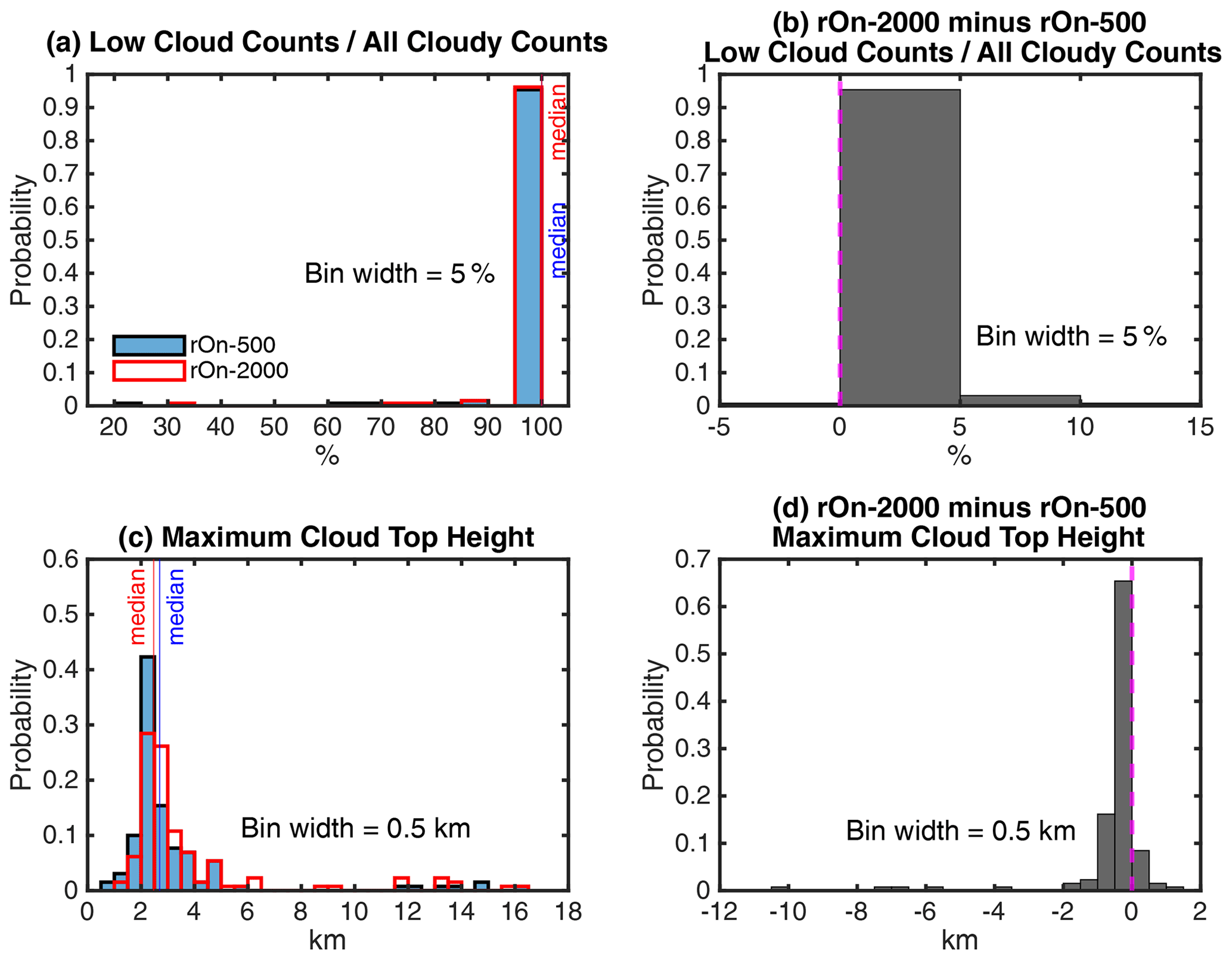
Figure 6 Similar to Fig. 5 but for histograms of the (a) low cloud (cloud top height <4 km) fractional contribution to the total number of cloudy columns (low cloud columns/all cloudy columns) and (c) the maximum cloud top height. The right column (b, d) represents rOn-2000 minus rOn-500 difference histograms for the corresponding fields (a, c) in the left column. The dashed magenta lines indicate where the difference between rOn-2000 and rOn-500 is zero. The median values of each characteristic are marked with vertical lines in the left column. The bin width of each histogram is marked in the upper corner of each panel.

Second, we analyze the distribution of maximum cloud top heights (Fig. 6c), and the differences as a result of aerosol loading (Fig. 6d). The maximum cloud top height is determined during the afternoon hours (12:00–18:00 LT) anywhere over land. This includes clouds both ahead of and along the sea breeze front. To identify cloud top heights, we start at the bottom of each model column and locate the lowest and highest level where the total condensate exceeds 0.1 g kg⁻¹. This column is then marked as a cloudy column when all the points between these two levels contain total condensate mixing ratios greater than 0.1 g kg⁻¹. We regard the highest level of the cloudy column as the convective cloud top height. This check on cloud contiguity means that we do not inadvertently take into account those situations in which there may be multiple clouds at different levels within the column.

The suppression of sea breeze convective intensity in rOn-2000, when compared with rOn-500, is evident in the reduction in the ensemble median of the maximum cloud top height (Fig. 6c). Negative values in Fig. 6d imply that the maximum cloud top height decreases with enhanced aerosol loading in the vast majority of simulations, most of which apply to low clouds (<4 km a.g.l.). However, there are some cases in which the cloud top heights increase in the presence of enhanced aerosol loading (Fig. 6d). It is evident from Fig. 6c that most of these enhancements in cloud top height with aerosol loading occur in association with the deep convective mode (>7 km a.g.l.). This is in spite of the fact that, while there are 12 cases with a deep convective mode in rOn-500, only 7 of these 12 cases have a deep convective mode when aerosol loading is enhanced in rOn-2000. Altogether, enhanced aerosol loading results in reduction in cloud top height of the low clouds (<4 km a.g.l.) but in a mixed response in the deep convective mode. As such, it appears that the impacts of increased aerosol on shallow cloud top heights are relatively robust and occur independently of the initial environment, whereas aerosol impacts on the deep convective cloud top heights vary as a function of the environment and, hence, are environmentally modulated.

5.2 Convective updraft velocities

In order to better understand the dynamical response of convection to enhanced aerosol loading, updrafts developing over land between 12:00 and 18:00 LT with velocities greater than 1 m s⁻¹ are analyzed. The maximum updraft velocity (Fig. 7a) represents the intensity of the most vigorous continental convection throughout each simulation. In all of the pristine and polluted ensemble simulations, the strongest updrafts are always found in association with the convergence along the sea breeze front, irrespective of whether the convection produced by this process is shallow or deep. To ensure that the maximum updrafts are convective (i.e., positively buoyant) and represent the intensity of sea-breeze-initiated convection, we take the maximum updrafts with a net positive instantaneous vertical acceleration contribution from the sum of the thermal buoyancy $\left(g\frac{\mathit{\theta }{}^{\prime }}{{\mathit{\theta }}_{\mathrm{0}}}+gr{{}^{\prime }}_{\mathrm{v}}\frac{\left(\mathrm{1}-\mathit{\epsilon }\right)}{\mathit{\epsilon }}\right)$ and condensate loading (−gr_c) terms in the following vertical momentum equation:

$${\displaystyle \frac{\partial w}{\partial t}}\approx g{\displaystyle \frac{{\mathit{\theta }}^{\prime }}{{\mathit{\theta }}_{\mathrm{0}}}}+g{r}_{\mathrm{v}}^{\prime }{\displaystyle \frac{\left(\mathrm{1}-\mathit{\epsilon }\right)}{\mathit{\epsilon }}}-g{r}_{\mathrm{c}}-{\displaystyle \frac{\mathrm{1}}{\mathit{\rho }}}{\displaystyle \frac{\partial p^{\prime }}{\partial z}}-w{\displaystyle \frac{\partial w}{\partial z}}-u{\displaystyle \frac{\partial w}{\partial x}}-v{\displaystyle \frac{\partial w}{\partial y}},$$

where w is vertical velocity, g is the gravitational acceleration of 9.8 m s⁻¹, θ^′ is the perturbation potential temperature, θ₀ is the base-state potential temperature, $r_v^{\prime }$ is the perturbation water vapor mixing ratio, ε is the ratio of dry air to water vapor gas constants, and r_c is the total condensate mixing ratio.

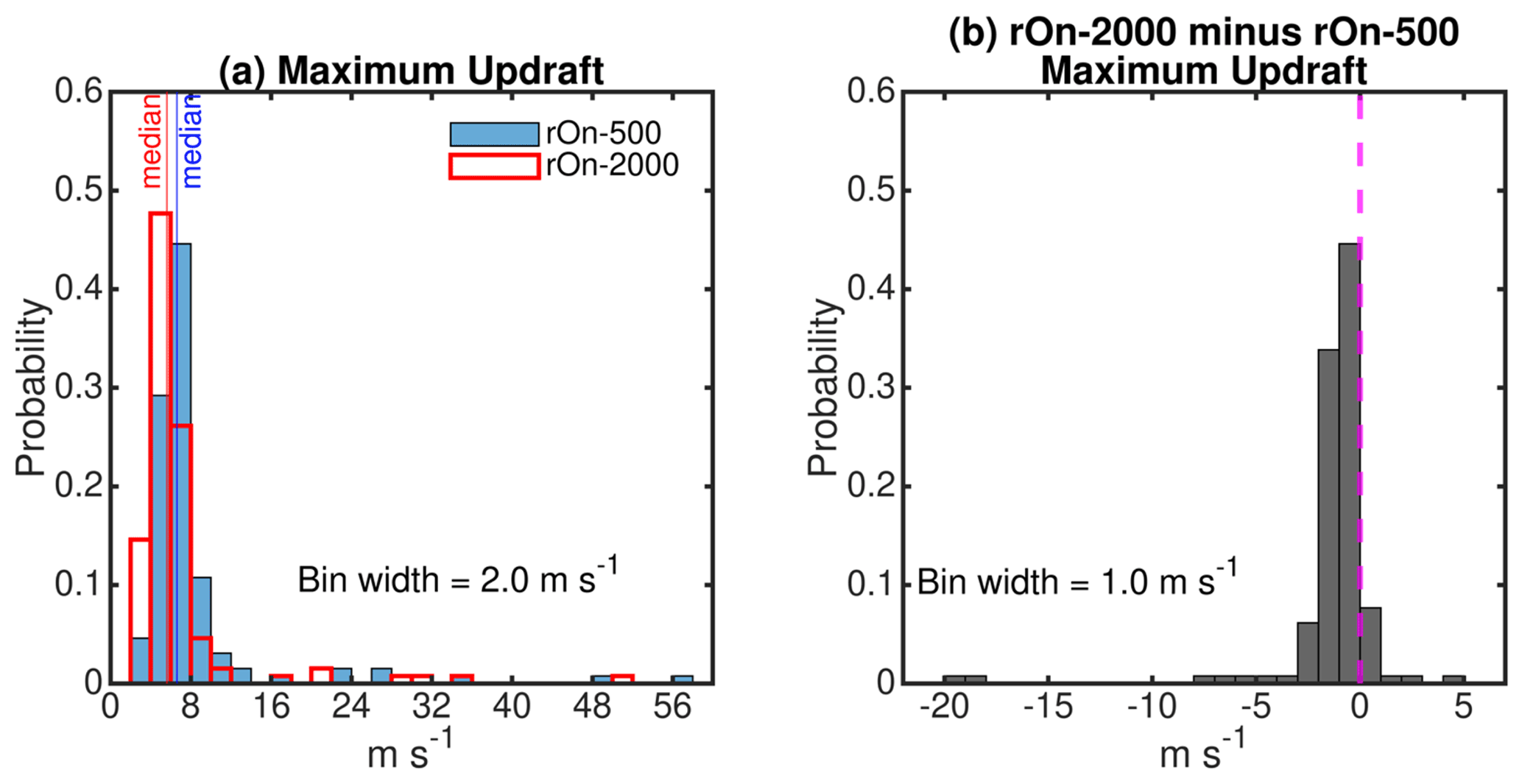
Figure 7 Similar to Fig. 5 but for (a) histograms of the maximum updraft velocity in rOn-500 and rOn-2000 and (b) a histogram of the maximum updraft velocity differences arising from aerosol loading (rOn-2000 minus rOn-500).

Overall aerosol-induced suppression of the maximum updraft velocities is evident by the decrease in the ensemble median values of the maximum updraft velocities (Fig. 7a). However, Fig. 7b implies that enhanced aerosol loading may produce either weaker or stronger updraft velocities, depending on the initial environmental conditions, and suggests that such aerosol-induced responses are environmentally modulated.

In the following subsections, we now seek to determine whether the key environmental parameters identified in Park et al. (2020b) as the predominant parameters driving the convective updrafts in rOn-500 are impacted by aerosol loading and, if so, why that is the case. We first examine both modes of the sea-breeze-initiated convection, followed by the daytime cumulus convection developing ahead of the sea breeze front. We examine these two types of convection separately, as they are driven by different processes, with sea breeze convergence and convective instability being critical to the sea-breeze-initiated convection and daytime surface heating and boundary layer mixing being important to the daytime cumulus developing ahead of the sea breeze.

5.2.1 Sea-breeze-initiated convective updrafts

Due to the steep vertical velocity gradients between the sea-breeze-initiated shallow and deep convective modes in rOn-500, Park et al. (2020b) found that constructing a statistically robust emulator for the maximum updraft velocities was not feasible. The same is true here for the rOn-2000 simulation, and thus, we have had to rely on other analysis methods to determine why deep convection is absent in 5 out of 12 cases in the polluted scenario. As noted in Park et al. (2020b), the 12 cases with sea-breeze-initiated deep modes in rOn-5000 all have initial boundary layer potential temperatures greater than 297 K as a common parameter. Given the range of initial boundary layer potential temperatures tested in this study (Table 2), this critical threshold for the deep mode falls at the upper end of this range and is the reason for why the vast majority of pristine ensemble members have shallow modes. Figure 8 shows scatterplots relating the maximum updraft velocity to the initial boundary layer potential temperature for all 130 ensemble members in rOn-500 (Fig. 8a) and rOn-2000 (Fig. 8b). It is clear from this figure that the sea-breeze-initiated deep convective mode (maximum cloud top height greater than 7 km) updrafts are in rOn-500 occurs in all of the ensemble members in which the initial boundary layer potential temperature is 297 K or greater, and in which the mixed layer CAPE is greatest (not shown). However, in rOn-2000 the threshold above which the deep convective mode occurs is 299 K, which is 2 K greater than that in rOn-500. For instance, while 4 of 12 deep convective simulations with the maximum updraft velocity greater than 10 m s⁻¹ have initial boundary layer potential temperatures between 297 and 299 K (Fig. 8a) in rOn-500, the only simulations in rOn-2000 with the maximum cloud top height greater than 7 km and the maximum updraft velocity greater than 10 m s⁻¹ occur for initial boundary layer potential temperature greater than or equal to 299 K (Fig. 8b). As demonstrated above, the surface temperatures are reduced in the presence of enhanced aerosol loading in the rOn-2000 ensemble due to aerosol direct effects, thereby reducing the convective potential in these simulations (Fig. 5f). Therefore, greater initial boundary layer potential temperatures are necessary to offset the aerosol-induced surface cooling in the polluted ensemble, thereby providing sufficient mixed layer CAPE to support the production of deep convection along the sea breeze front. Also, if we consider those simulations with the same initial boundary layer potential temperatures, the presence of aerosol reduces deep convection initiation. This is due to the fact that aerosol loading leads to less deep convection initiation due to reduced surface temperatures through the scattering of surface downwelling shortwave radiation by aerosol particles.

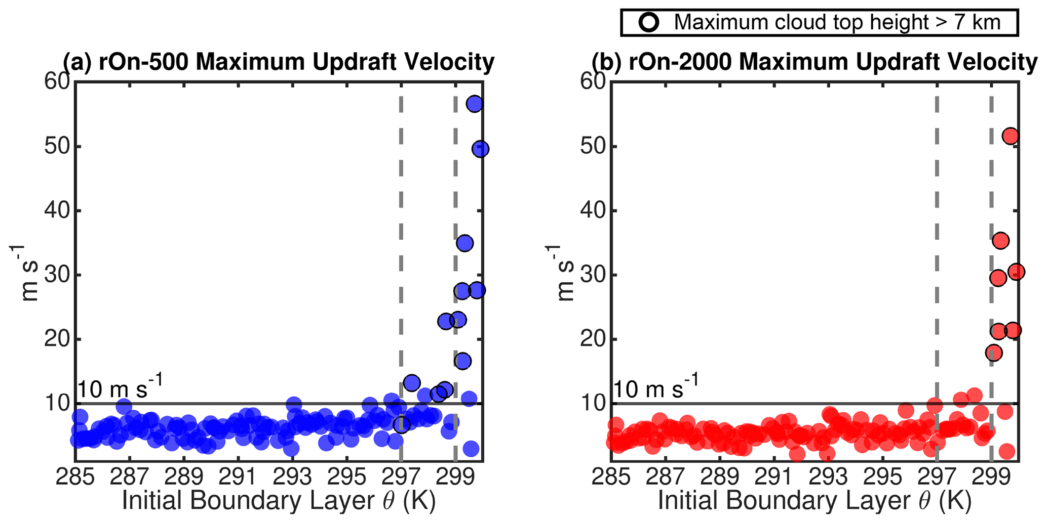
Figure 8 Pairwise scatterplots for the maximum updraft velocity (m s⁻¹) versus the initial boundary layer potential temperature (K) for the (a) rOn-500 and (b) rOn-2000 ensembles. The vertical dashed gray lines refer to the potential temperature thresholds described in the text. Simulations with deep convection, identified by the maximum cloud top height >7 km, are marked with black circles.

5.2.2 Daytime cumulus convection updrafts

Unlike the sea-breeze-initiated convective updrafts, constructing a robust emulator was possible for the updraft velocities of the daytime cumulus convection forming ahead of sea breeze front. We can therefore draw on the emulator results in our analysis of these updrafts. The bar graphs in Fig. 9a (rOn-500) and b (rOn-2000) indicate how much of the variance in the median updraft velocity is explained by the individual perturbations to the 10 environmental parameters tested. Each stacked bar graph's height refers to the summation of first-order contributions of the 10 parameters to the median updraft velocity. Any blank space remaining above the bar indicates the contributions made by higher-order interactions involving multiple parameters. It is evident from the left-most bar graph (labeled “Overall”) that the same two parameters, the soil saturation fraction (dark gray) and the inversion layer strength (pink), are the predominant contributors to the median updraft velocities in rOn-500 and rOn-2000, although their percentage contributions differ. In order to understand the impacts of aerosols on these relative contributions, we first need to understand the processes driving these two predominant contributions.

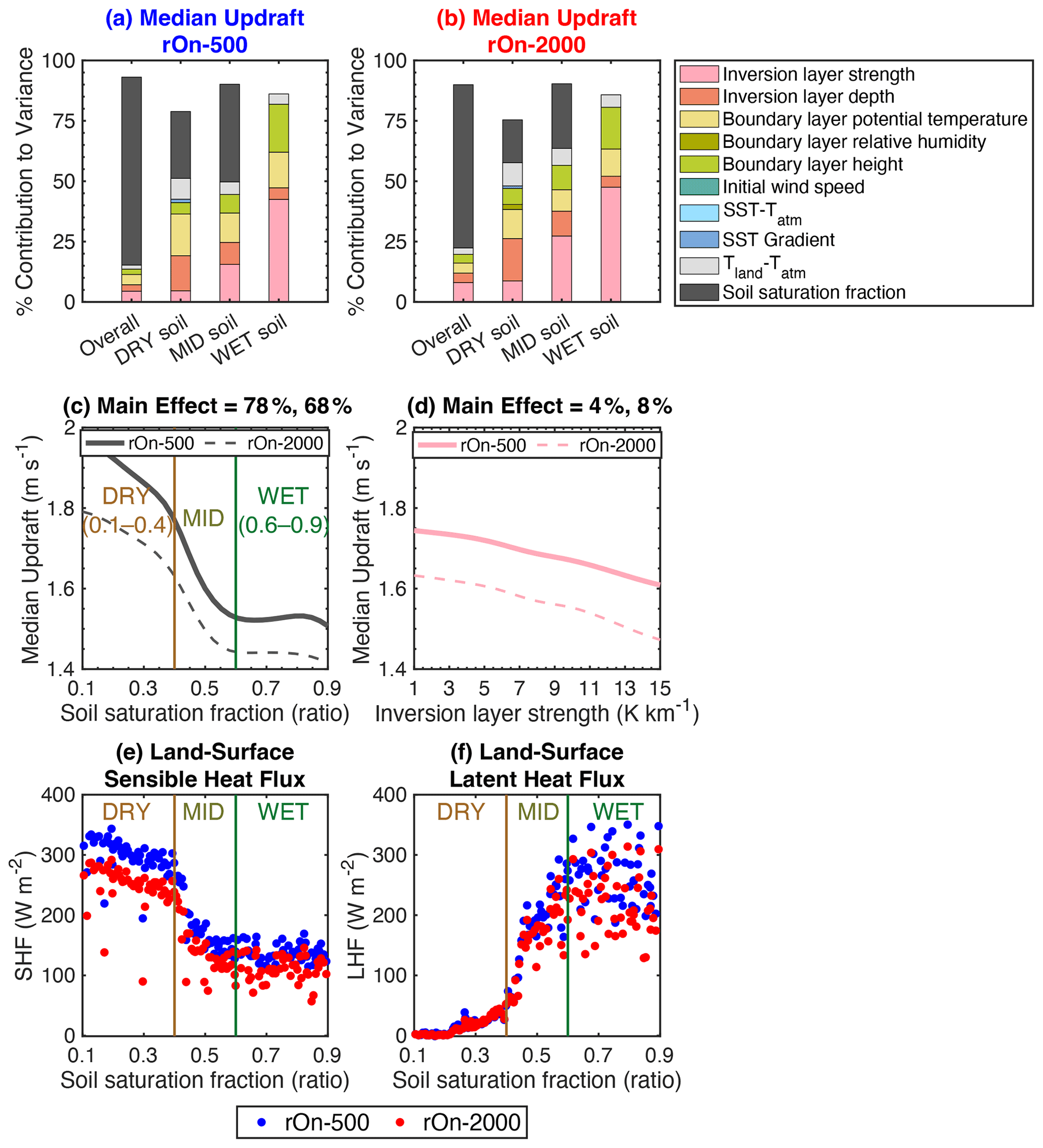
Figure 9 The percentage contribution to the variance of median updraft velocities in (a) rOn-500 and (b) rOn-2000 by each of the 10 environmental parameters of interest over the entire parameter space range (left stacked bar graphs) and then over the DRY, MID, and WET soil regimes (second to fourth stacked bar graphs from the left). Mean responses of the median updraft velocities to the two most important parameters, i.e., (c) soil saturation fraction and (d) inversion layer strength. Solid and dashed lines in panels (c) and (d) indicate the mean responses of the median updraft velocities of rOn-500 and rOn-2000, respectively. The numbers at the top of each plot in panels (c) and (d) indicate the percentage contribution of each parameter to the output variance. (e) Pairwise scatterplots of land-averaged surface sensible heat flux between 12:00 and 18:00 LT (W m⁻²) and soil saturation fraction are shown. Blue and red colors indicate rOn-500 and rOn-2000, respectively. Panel (f) is the same as panel (e) but for land-averaged latent heat flux (W m⁻²). Note that 130 points in panels (e) and (f) have different values for the 10 perturbed environmental parameters.

Figure 9c and d present the mean responses of the emulator-predicted median updraft velocities to the soil saturation fraction and inversion layer strength. It is clear from these figures that drier soils and weaker inversion layers promote more vigorous daytime cumulus convection in both the pristine and polluted regimes. While the response of the updraft velocities to the strength of the inversion layer is a relatively simple, continuously decreasing function, the sensitivity of the median updraft velocities to the soil saturation fraction (Fig. 9c) shows the following three relatively distinct regimes: (1) moderate velocity changes for soil saturation fractions between 0.1 and 0.4, (2) large velocity changes for soil saturation fractions between 0.4 and 0.6, and (3) relatively neutral velocity responses for soil saturation fractions between 0.6 and 0.9. We will refer to these three regimes as the DRY, MID, and WET soil moisture regimes based on the response curve in Fig. 9c. It should be noted that sandy clay loam's observed soil saturation fraction varies from 0.25 to 0.75 along coastal equatorial Africa in June, July, and August (Rodell et al., 2004). Here we have extended the range tested to 0.1 through 0.9 to encompass slightly drier and wetter soil conditions in addition to those reported by Rodell et al. (2004) to take into account potentially more extreme conditions anticipated with changing climates. The corresponding variance-based sensitivity analyses for the daytime cumulus convection stratified by these three different soil regimes are shown in the second to fourth bar graphs from the left in Fig. 9a and b.

To understand the median updraft velocity responses in the soil moisture regimes, one needs to note that the soil saturation fraction value of 0.4, which separates the DRY and MID soil moisture regimes, corresponds to the permanent wilting point of sandy clay loam soil. The permanent wilting point is the minimum amount of soil moisture that a plant's roots require in order not to permanently wilt. Below the permanent wilting point, the vegetation becomes stressed, resulting in a shutdown of evapotranspiration and thereby suppressing the release of water vapor (Hohenegger and Stevens, 2018; Drager et al 2020). In the DRY soil regime (0.1–0.4), where the soil moisture falls below that of the permanent wilting point, the surface latent heat flux is suppressed (Fig. 9f), and more of the surface heating goes into enhancing the sensible heat fluxes (Fig. 9e). The relatively strong sensible heat fluxes in the DRY regime contribute to warmer, deeper boundary layers and, hence, the stronger updraft velocities observed in this regime (Fig. 9c). Over the WET soil regime (0.6–0.9), with abundant evaporation and transpiration, the surface sensible heat flux is reduced and the surface latent heat flux is enhanced (Fig. 9e and f) when compared with the DRY soil regime. Furthermore, the surface sensible heat flux is no longer sensitive to the soil saturation fraction, as is evident in the flat gradient of the curve in Fig. 9e and in the absence of the soil saturation fraction contributions to the WET regime in Fig. 9a and b (fourth bar graph from the left). The updrafts within the WET soil regime are therefore weaker than the DRY and MID regimes. Finally, in the MID soil regime, both the sensible and latent heat fluxes show the most sensitive responses to changes in the soil saturation fraction (Fig. 9e and f). While the median updraft velocities (Fig. 9c) and surface sensible heat flux (Fig. 9e) are similar in trend to those over the DRY soil regime, the slopes are steeper in the MID soil regime. As such, the relative importance of the soil saturation fraction in contributing to updraft velocity variance is greatest in the MID soil regimes compared with the DRY or WET soil regimes (second to fourth bar graphs from the left in Fig. 9a and b). Drager et al. (2020) also noticed nonlinear responses to soil moisture focused around the permanent wilting point in their study of soil moisture impacts on cold pools.

We now turn to the impacts of enhanced aerosol loading on the roles of the soil saturation fraction and the inversion layer strength. When comparing Fig. 9a with b, the relative percentage contribution of soil saturation fraction to updraft variability decreases from 78 % to 68 % with enhanced aerosol loading, whereas that of the inversion layer strength increases from 4 % to 8 %. The soil saturation fraction plays an important role in the daytime cumulus convection ahead of the sea breeze front through its control of the magnitude of the surface sensible and latent heat fluxes and its partitioning between them. As discussed in Sect. 4, the aerosol-induced reduction in surface downwelling shortwave radiation in the polluted ensemble reduces the incoming shortwave radiation, the surface longwave emission, the associated surface sensible and latent heat fluxes, and the mixed layer depth. The reduction in the percentage contributions of the overall soil saturation fraction to the median updraft velocities in the polluted ensemble (compare left bars in Fig. 9a and b) therefore reflects this reduced role of the surface fluxes and boundary layer mixing in driving the updrafts. When examining aerosol impacts on the specific soil moisture regimes (three bars on the right of Fig. 9a and b), it is clear that under conditions of enhanced aerosol loading the relative importance of soil saturation fraction on the median updraft is reduced in the DRY and MID soil regimes, while it is completely absent in WET soil regimes regardless of aerosol loading. Comparing the emulator-predicted median updrafts between the pristine and polluted conditions (Fig. 9c), the trends in the relationship between the soil saturation fraction and the updraft velocities are very similar, but median updrafts are stronger in rOn-500 due to the stronger sensible heat fluxes.

In rOn-500, inversion layer strength is the second most important parameter for the mixed-layer depth and the median updraft velocity. When the initial inversion layer is weaker, the lower troposphere is less stable, which promotes daytime turbulent mixing and leads to stronger vertical motions. While the inversion layer is still the second most important parameter for the median updraft in rOn-2000, its relative importance is increased from 4 % to 8 %. As the contributions made by the rest of the factors to the velocity variance remain much the same between the pristine and polluted conditions (Fig. 9a and b), this increase primarily reflects the reduced contribution by the soil saturation fraction and the concomitant increase in the contribution of the inversion layer strength to boundary layer development and, hence, to boundary layer updrafts.

5.3 Surface accumulated precipitation

The changes in surface accumulated precipitation with increased aerosol loading are now analyzed. Figure 10 displays a histogram of the aerosol-induced differences in the land-averaged accumulated surface precipitation at 18:00 LT between rOn-2000 and rOn-500. The percentage differences are only determined for those simulations that produce at least 0.1 mm of land-averaged accumulated precipitation in rOn-500 (36 out of 130 simulations). Only 19 simulations produce more than 0.1 mm of area-averaged precipitation in both rOn-500 and rOn-2000, and no simulation in rOn-2000 produces more than 0.1 mm of precipitation when its corresponding ensemble member in rOn-500 does not produce precipitation. Figure 10 distinctly shows that the accumulated precipitation is reduced in all of the rOn-2000 precipitating ensemble members when compared with their corresponding counterparts in rOn-500, thereby demonstrating that the enhanced aerosol loading leads to an overall reduction in surface precipitation produced by the sea breeze system, irrespective of the environment. The bulk microphysical processes contributing to the differences in the surface rainfall in the 36 precipitating ensemble pairs are shown in Fig. 11. All of the following source and sink terms for rain are considered:

1. Cloud to rain – cloud water transferred to rain through collection (gain term; Fig. 11a)

2. Rain to vapor – evaporation of liquid water from rain (loss term; Fig. 11b)

3. Melting of ice – ice mass transferred to rain via thermodynamic melting as the ice species fall below the freezing level (gain term; Fig. 11c)

4. Rain to ice – rainwater that is collected by ice species through riming (loss term; Fig. 11d)

5. Ice to rain – collisional ice melting due to collection of warmer rain (gain term; Fig. 11e).

These process rates are averaged across all grid points over the land domain between 12:00 and 18:00 LT. In most of the precipitating members, the cloud frequency over land is heavily weighted by the daytime cumulus convection mode. As a result, the frequency and associated contributions made by the averaged mixed-phased process contributions are small, if they even exist. However, in some members, as shown in Fig. 11c–e, the averaged mixed-phase process contributions are greater than warm-phase process. As most of the differences in the processes contributing to differences in surface rainfall occur below 10 km a.g.l., we restrict the axes in Fig. 11 to between the surface and 10 km a.g.l. to enhance figure clarity. It should also be noted that the freezing level varies from simulation to simulation due to the different initial temperature and moisture profiles. For example, two of 36 precipitating pairs have a freezing level (averaged over the land domain and during the afternoon) of 1.64 and 2.12 km in rOn-500, respectively. These lower freezing levels are primarily due to their initial boundary layer potential temperature being at the lower end of the range being tested. It is evident in all simulations, regardless of the different initial conditions, that the average warm rain production rates (i.e., cloud to rain) are greater in rOn-500 than rOn-2000 (Fig. 11a). Similarly, average rain evaporation rates (i.e., rain to vapor) shown in Fig. 11b are also greater in magnitude in rOn-500 than rOn-2000, demonstrating that the population of less numerous but larger raindrops formed in rOn-2000 (Fig. 11f) evaporate less readily. The production of populations of fewer but larger raindrops in polluted conditions has been observed previously (e.g., Altaratz et al., 2008; Storer and van den Heever, 2013). Figure 11 therefore demonstrates that, in the mean, precipitation suppression in the polluted environment primarily occurs as a result of the suppression of warm rain formation. Furthermore, as this response is evident across all 36 precipitating members, it appears that these warm rain trends occur independent of the environmental conditions, although the magnitudes in the response certainly do vary with environment. Figure 11c–e show that enhanced aerosol loading primarily produces a reduction in all three of the cold rain processes contributing to the rain budget, with only minor increases with aerosol loading in some cases. However, given the small sample size, additional testing would be required before conclusive statements can be made regarding environmental modulation of cold phase processes.

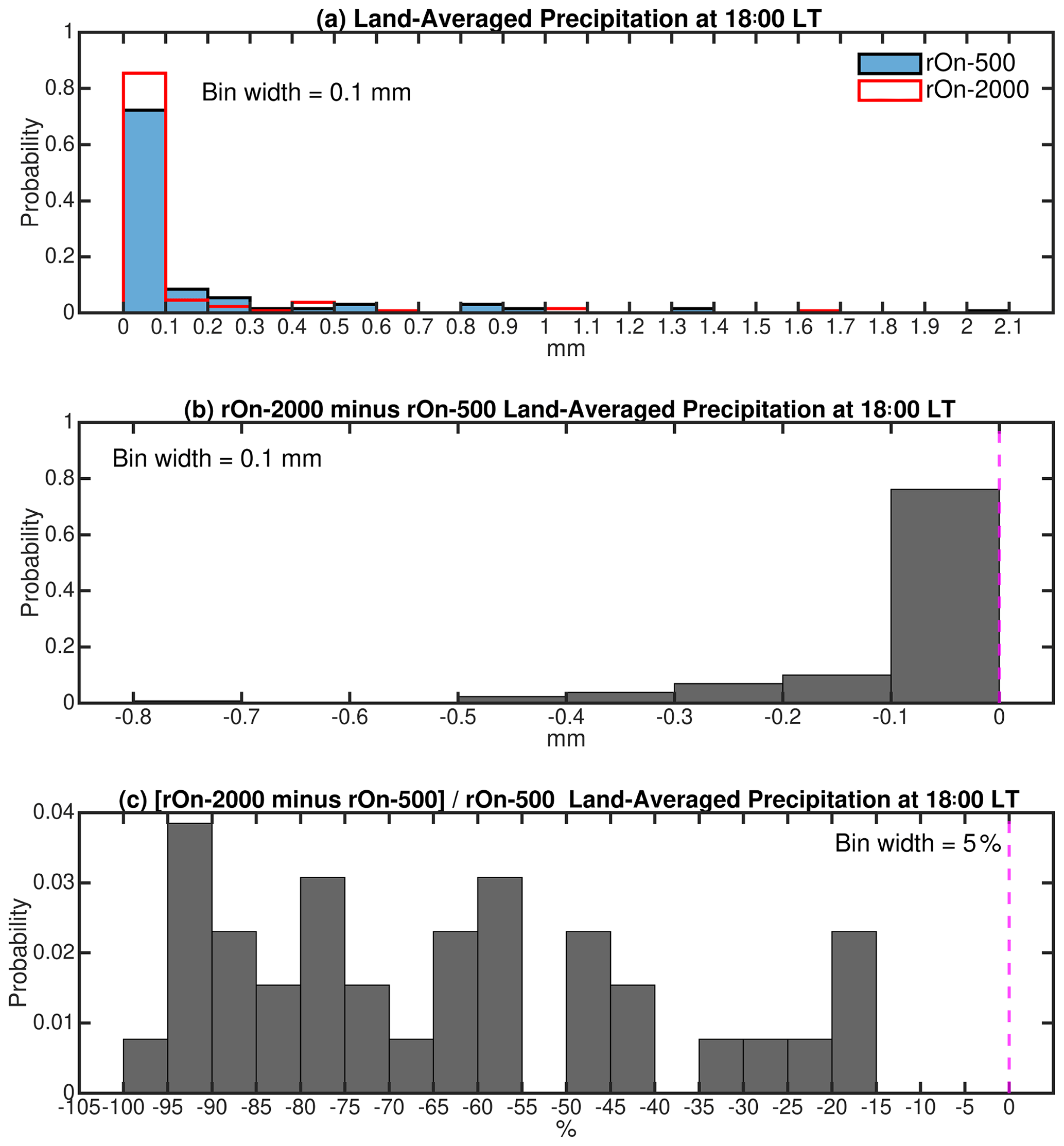
Figure 10 (a) A histogram of the land-averaged accumulated surface precipitation at sunset (18:00 LT) in rOn-500 (blue) and in rOn-2000 (red) for simulations that produce at least 0.1 mm of the land-averaged accumulated precipitation in rOn-500. The absolute and percent differences between rOn-500 and rOn-2000 are shown in panels (b) and (c), respectively, where the percentage differences are with respect to rOn-500. The dashed magenta line in panels (b) and (c) indicates where the difference between rOn-2000 and rOn-500 is zero. The bin width of the histogram is marked in each panel.

Figure 11 Aerosol-induced differences to the processes generating rain for the range of environmental conditions tested in these large ensemble experiments. Shown are the rOn-2000 minus rOn-500 differences, for (a) cloud to rain, (b) rain to vapor, (c) melting of ice, (d) rain to ice, and (e) ice to rain rates (see the text for an explanation of these processes), using the 36 ensemble pairs that produce at least 0.1 mm of land-averaged surface accumulated precipitation in rOn-500. Process rates are averaged over the land domain between 12:00 and 18:00 LT. (f) The rOn-2000 minus rOn-500 raindrop diameter averaged over the land between 12:00 and 18:00 LT. The thin black lines in all of the figures are from all 36 pairs, and the thick gray lines in panels (a) and (b) are the means of the rOn-2000 minus rOn-500 for the 36 pairs. The dashed magenta lines indicate where the difference between rOn-2000 and rOn-500 is zero.

6 Summary and discussion

The primary goals of this study have been (1) to investigate how microphysically and radiatively active aerosol particles influence the wide range of convective environments supporting sea breeze convective regimes and the convective cloud characteristics developing under these regimes and (2) to determine whether the convective environment modulates these aerosol impacts on the convection. In order to achieve our goals, we conducted two large numerical model ensembles, where the only difference between the ensembles was the aerosol loading. Each of these two ensembles was comprised of 130 members initialized with 130 different initial conditions, representing the simultaneous perturbation of 10 thermodynamic, wind, and surface properties, the ranges of which were sourced where possible from the current sea breeze literature. The selection of these 130 initial conditions was based on a statistical space-filling method (Morris and Mitchell, 1995), and the pristine (rOn-500) and polluted (rOn-2000) ensembles were then compared using the statistical emulator framework developed by Johnson et al. (2015).

The comparison between rOn-500 and rOn-2000 demonstrated that aerosol direct effects resulted in less shortwave radiation reaching the surface. The associated longwave emission from the land surface was also reduced, thereby producing a cooler land surface, a smaller land–sea thermal contrast, and a weaker sea breeze circulation. In the presence of aerosol direct effects, the ensemble median values of the land surface latent heat fluxes, the surface-based mixed layer depth, the mixed-layer CAPE, the maximum sea breeze inland extent, and the maximum frontal updraft were subsequently reduced in the polluted scenario. However, this aerosol-induced reduction was not always found across all of the simulations comprising the ensembles. Furthermore, the magnitude of the reduction varied as a function of the initial environmental condition. Therefore, while these ensembles indicate that less favorable environments for sea breeze convective systems frequently resulted from enhanced aerosol loading, the surface, wind, and low-level thermodynamic conditions may occasionally modulate aerosol impacts on the convective environment. These results extend those of Grant and van den Heever (2014), in which a similar sensitivity of tropical sea breeze convection to aerosol loading was demonstrated, albeit for only one set of initial conditions.

The resulting aerosol-induced changes in convection over land in the afternoon (12:00–18:00 LT) were then examined for the clouds comprising the sea breeze system, including those clouds forming both ahead of and along the sea breeze front. Overall, the sea-breeze-initiated convection remained stronger and deeper than daytime cumulus convection forming ahead of the sea breeze front. The shallow mode of the sea-breeze-initiated convection showed an overall reduction in maximum cloud top height and maximum updraft velocity with enhanced aerosol loading, despite different initial environmental conditions, suggesting that the aerosol-induced suppression of shallow convective velocities is robust for the wide range of surface, wind, and low-level thermodynamic conditions tested here. However, both the sign and magnitude of the changes to the sea-breeze-initiated deep convective mode in response to enhanced aerosol loading varied as a function of initial environmental conditions, with some ensemble members showing an increase in updraft velocity, while others showed a decrease or no change to the strength of the updraft. This demonstrates that aerosol impacts on the deep convective updrafts developing within these large ensembles are environmentally modulated. Of the 10 environmental parameters perturbed in the initial conditions, the initial boundary layer potential temperature was shown to have important implications for the deep convective mode. The sea-breeze-initiated deep mode was only observed in those rOn-2000 ensemble simulations in which the initial boundary layer potential temperatures were greater than 299 K, compared with a corresponding threshold of 297 K in rOn-500. With enhanced aerosol loading inducing cooler and more stable near-surface environments in rOn-2000, the warmer initial boundary layer potential temperatures were found to be necessary to facilitate deep convection through higher mixed layer CAPE.

The aerosol-induced reduction in surface fluxes and mixed-layer depth led to the suppression of daytime cumulus convection ahead of the sea breeze front, irrespective of the different initial conditions, and thus appears to be a robust response. A 10-dimensional variance-based sensitivity analysis, combined with statistical emulation, revealed that the relative importance of the soil saturation fraction on the surface fluxes and mixed layer depth, and hence on the daytime cumulus updrafts, was reduced in the presence of enhanced aerosol loading. A nonlinear sensitivity of boundary layer updraft velocities to soil saturation fraction was also found, with the greatest convective updraft response observed in the MID soil saturation fraction regime, followed by a moderate response in the DRY soil saturation fraction regime and little response in the WET soil regime. These sensitivities were found to exist in both the pristine and polluted environments. The sensitivity analysis results therefore emphasize the importance of considering atmosphere–radiation–land feedback processes in the modeling studies of aerosol–cloud interactions.

Finally, changes in the surface-accumulated precipitation to increased aerosol loading were analyzed. Again, a consistent aerosol-induced reduction was observed across the entire ensemble of model simulations. Spatiotemporally averaged warm rain production and evaporation rates exhibited robust aerosol-induced behaviors across the ensembles. While the trends in precipitation reduction were found to be consistent irrespective of the environment, the magnitude of precipitation suppression was found to be modulated by surface, wind, and low-level thermodynamic environments. Cold rain processes also showed an overall aerosol-induced reduction; however, given the small sample size, the robustness of these trends is uncertain and would require additional experiments before more definitive statements can be made.

In spite of the large ensembles conducted and analyzed in this study, there are a number of shortfalls that should be addressed in future studies. First, we only tested a single aerosol species, i.e., ammonium sulfate, which is a strong scatterer but a less efficient absorber of radiation. It is worth noting that more strongly absorbing aerosols, such as mineral dust or smoke, are also substantial contributors to aerosol emissions in equatorial Africa (Adams et al., 2012; Chakraborty et al., 2015). The potential importance of the interactions of absorbing aerosol with radiation and microphysics has been reported in previous studies. For instance, Saide et al. (2015) found that smoke absorption tends to either burn off clouds or enhance the capping inversion, depending on the smoke's location. Such radiation absorption in the presence of other aerosol species may therefore produce different effects on sea breeze convection to those reported here for sulfate. This study's perturbed parameter ensemble approach could be extended to such studies considering absorbing aerosol species. Second, only two different aerosol loadings were examined in this study. Some modeling studies have reported non-monotonic responses of convective clouds and precipitation to enhanced aerosol loading (Storer and van den Heever, 2013; Dagan et al., 2017; Liu et al., 2019). As such, a future study should assess the potential nonlinear effects of aerosol on convection across a wide range of surface and meteorological environments by conducting ensembles with a broader range of aerosol loadings. Third, a grid spacing of 1 km was selected for these extensive ensembles given their high computational costs. Such a grid spacing will marginally resolve deep convective cloud systems but will under-resolve the shallow convective mode. As computational capabilities are enhanced, a similar study should be conducted using grid spacings of 𝒪(100 m).

Many of the past studies assessing aerosol impacts on deep convection have tended to neglect the role of aerosol direct forcing in order to focus on aerosol indirect effects. However, our results indicate the importance of considering both aerosol direct and indirect effects when determining the impacts of aerosols on convective systems and suggest that future studies should consider both aerosol direct and indirect effects to fully understand aerosol impacts on deep convection. A subset comprised of the members of the pristine and polluted ensembles that produced deep convection has been further analyzed to assess the relative roles of aerosol direct and indirect effects specifically on deep convection, as well as to assess the robustness of warm and cold phase invigoration under varying environments, and will be published elsewhere. Finally, the environmental modulation of both direct and indirect aerosol effects on tropical sea breeze convective systems demonstrated here highlights the need to examine such impacts across the wide range of convective environments supporting other types of organized convective systems.