the Creative Commons Attribution 4.0 License.
the Creative Commons Attribution 4.0 License.
 | 02 Jun 2021
New methodology shows short atmospheric lifetimes of oxidized sulfur and nitrogen due to dry deposition
Katherine Hayden
Paul Makar
John Liggio
Samar G. Moussa
Ayodeji Akingunola
Robert McLaren
Ralf M. Staebler
Andrea Darlington
Jason O'Brien
Junhua Zhang
Mengistu Wolde
Leiming Zhang
The atmospheric lifetimes of pollutants determine their impacts on human health, ecosystems and climate, and yet, pollutant lifetimes due to dry deposition over large regions have not been determined from measurements. Here, a new methodology based on aircraft observations is used to determine the lifetimes of oxidized sulfur and nitrogen due to dry deposition over km2 of boreal forest in Canada. Dry deposition fluxes decreased exponentially with distance from the Athabasca oil sands sources, located in northern Alberta, resulting in lifetimes of 2.2–26 h. Fluxes were 2–14 and 1–18 times higher than model estimates for oxidized sulfur and nitrogen, respectively, indicating dry deposition velocities which were 1.2–5.4 times higher than those computed for models. A Monte Carlo analysis with five commonly used inferential dry deposition algorithms indicates that such model underestimates of dry deposition velocity are typical. These findings indicate that deposition to vegetation surfaces is likely underestimated in regional and global chemical transport models regardless of the model algorithm used. The model–observation gaps may be reduced if surface pH and quasi-laminar and aerodynamic resistances in algorithms are optimized as shown in the Monte Carlo analysis. Assessing the air quality and climate impacts of atmospheric pollutants on regional and global scales requires improved measurement-based understanding of atmospheric lifetimes of these pollutants.
- Article
(5632 KB) - Full-text XML
-
Supplement
(1153 KB) - BibTeX
- EndNote


Deposition represents the terminating process for most air pollutants and the starting point for ecosystem impacts. Understanding deposition is critical in determining the atmospheric lifetimes and spatial scales of atmospheric transport of pollutants, which in turn dictates their ecosystem (WHO, 2016; Solomon et al., 2007) and climate (Samset et al., 2014) impacts. In particular, atmospheric lifetimes (τ) of oxidized sulfur and nitrogen compounds influence their concentrations and column burdens in air, which affect air quality and hence human exposure (WHO, 2016). Furthermore, the lifetime of these species affects their contributions to atmospheric aerosols, with a consequent influence on climate via changes to radiative transfer through scattering and cloud formation (Solomon et al., 2007). In addition, their deposition can exceed critical load thresholds, causing aquatic and terrestrial acidification and eutrophication in the case of nitrogen deposition (Howarth, 2008; Bobbink et al., 2010; Doney, 2010; Vet et al., 2014; Wright et al., 2018). Quantifying τ and deposition thus provides a crucial assessment of these regional and global impacts.
Deposition occurs through wet and dry processes. While wet deposition fluxes can be measured directly (Vet et al., 2014), there are few validated methods for dry deposition fluxes (Wesley and Hicks, 2000) and none which estimates deposition over large regions. Dry deposition fluxes (F) may be obtained using micrometeorological measurements for pollutants for which fast-response instruments are available. However, these results are only valid for the footprints of the observation sites, typically hundreds of metres (Aubinet et al., 2012), and their extrapolation to larger regions may suffer from representativeness issues. As a result, atmospheric lifetimes τ with respect to dry deposition have not been determined through direct observations. On a regional scale, dry deposition fluxes are typically derived using an inferential approach by multiplying network-measured or model-predicted air concentrations with dry deposition velocities (Vd) (Sickles and Shadwick, 2015; Fowler et al., 2009; Meyers et al., 1991), which are derived using resistance-based inferential dry deposition algorithms (Wu et al., 2018) and compared with limited micrometeorological flux measurements (Wesley and Hicks, 2000; Wu et al., 2018; Finkelstein et al., 2000; Matsuda et al., 2006; Makar et al., 2018) for validation. When applied to a regional scale, an inferential-algorithm-derived Vd may have significant uncertainties (Wesley and Hicks, 2000; Aubinet et al., 2012; Wu et al., 2018; Finkelstein et al., 2000; Matsuda et al., 2006; Makar et al., 2018; Brook et al., 1997). For example, inferred Vd for SO2, despite being the most studied and best estimated, may be underestimated by 35 % for forest canopies (Finkelstein et al., 2000). Underestimated Vd for SO2 and nitrogen oxides can contribute to model overprediction of regional and global SO2 concentrations (Solomon et al., 2007; Christian et al., 2015; Chin et al., 2000) or underprediction of global oxidized nitrogen dry deposition fluxes (Paulot et al., 2018; Dentener et al., 2006).
Here, a new approach is presented to determine τ with respect to dry deposition and F for total oxidized sulfur (TOS, the sulfur mass in SO2 and particle SO4 – pSO4) and total reactive oxidized nitrogen (TON, the nitrogen mass in NO, NO2, and others designated as NOz) on a spatial scale of km2, using aircraft measurements. This approach provides a unique methodology to determine τ and F over a large region. Coupled with analyses for chemical reaction rates (for TOS compounds), the average Vd for TOS and TON over the same spatial scale was also determined. The airborne measurements were obtained during an intensive campaign from August to September 2013 in the Athabasca Oil Sands Region (AOSR) (Gordon et al., 2015; Liggio et al., 2016; Li et al., 2017; Baray et al., 2018; Liggio et al., 2019) in northern Alberta, Canada. Direct comparisons with modelled dry deposition estimates are made to assess their uncertainties and the spatial–temporal scales of air pollutant impacts.
2.1 Lagrangian flight design
Details of the airborne measurement program have been described elsewhere (Gordon et al., 2015; Liggio et al., 2016; Li et al., 2017; Liggio et al., 2019; Baray et al., 2018). Briefly, an instrumented National Research Council of Canada Convair-580 research aircraft was flown over the AOSR in Alberta, Canada, from 13 August to 7 September 2013. The flights were designed to determine emissions from mining activities in the AOSR, assess their atmospheric transformation processes and gather data for satellite and numerical model validation. Three flights were flown to study transformation and deposition processes by flying a Lagrangian pattern so that the same pollutant air mass was sampled at different time intervals downwind of emission sources for a total of 4–5 h and up to 107–135 km downwind of the AOSR sources. Flights 7 (F7, 19 August), 19 (F19, 4 September) and 20 (F20, 5 September) took place during the afternoon when the boundary layer was well established. The flights were conducted in clear-sky conditions, so wet deposition processes were insignificant. As shown in Fig. 1, the aircraft flew tracks perpendicular to the oil sands plume at multiple altitudes between 150 and 1400 m a.g.l. and multiple intercepts of the same plume downwind. Vertical profiles conducted as spirals were flown at the centre of the plume which provided information on the boundary layer height and extent of plume mixing. The flight tracks closest to the AOSR intercepted the main emissions from the oil sands operations; there were no other anthropogenic sources as the aircraft flew further downwind of the AOSR.
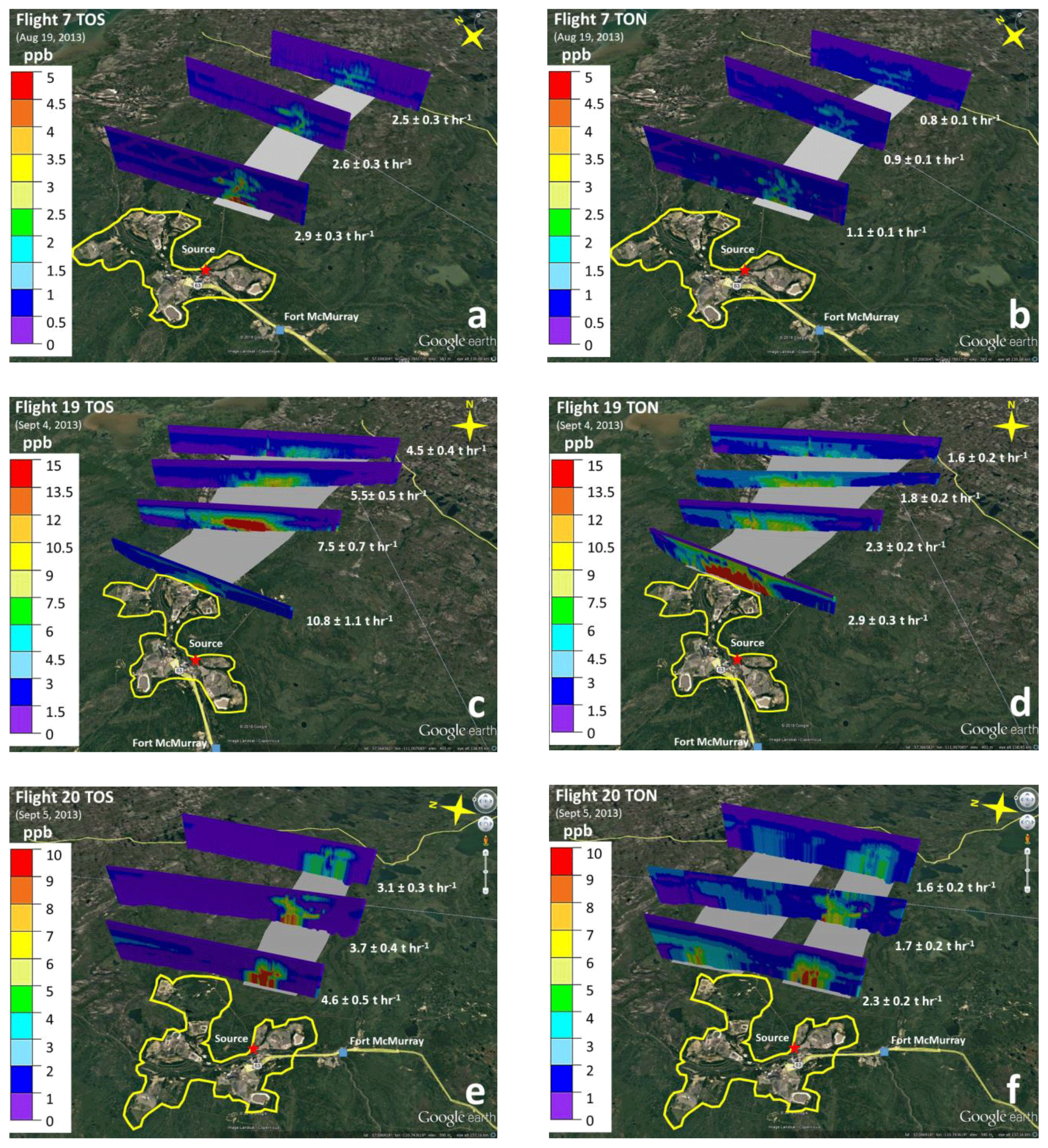
Figure 1TOS (total oxidized sulfur) and TON (total oxidized nitrogen) plumes downwind of the AOSR during three Lagrangian flights, F7, F19 and F20. The AOSR facilities are enclosed by the yellow outline. The transfer rates T in t S or N h−1 across each screen are shown. The grey-shaded surface areas are identified as the geographic footprint under the plumes. Data: Google Image © 2018 Image Landsat/Copernicus.
2.2 Aircraft measurements
A comprehensive suite of detailed gas- and particle-phase measurements was made from the aircraft. Measurements pertaining to the analysis in this paper are discussed below.
-
SO2 and NOy. Ambient air was drawn in through a 6.35 mm (”) diameter perfluoroalkoxy (PFA) sampling line taken from a rear-facing inlet located on the roof towards the rear of the aircraft. The inlet was pressure-controlled to 770 mm Hg using a combination of a MKS pressure controller and a Teflon pump. Ambient air from the pressure-controlled inlet was fed to instrumentation for measuring SO2 and NOy. The total sample flow rate was measured at 4988 cm3 min−1, of which SO2 and NOy were 429 and 1085 cm3 min−1, respectively. SO2 was detected via pulsed fluorescence with a Thermo 43iTLE (Thermo Fisher Scientific, Franklin, MA, USA). NOy (also denoted as TON) was measured by passing ambient air across a heated (325 ∘C) molybdenum converter that reduces reactive nitrogen oxide species to NO. NO was then detected through chemiluminescence with a modified Thermo 42iTL (Thermo Fisher Scientific, Franklin, MA, USA) run in NOy mode. An inlet filter was used for SO2 to exclude particles, but NOy was not filtered prior to the molybdenum converter. NOy includes NO, NO2, HNO3 and other oxides of nitrogen such as peroxy acetyl nitrate and organic nitrates (Dunlea et al., 2007; Williams et al., 1998). Although there was no filter on the NOy inlet to exclude particles, the inlet was not designed to sample particles (i.e. rear-facing PFA tubing). As a result, pNO3 was not included as part of NOy (TON). The conversion efficiency of the heated molybdenum converter and inlet transmission was evaluated with NO2 and HNO3 and found to be near 100 % and >90 %, respectively. Previous studies conducted by Williams et al. (1998) showed similar molybdenum converter efficiencies, including that of n-propyl nitrate near 100 %. Interferences from alkenes or NH3 were assumed to be negligible (Williams et al., 1998; Dunlea et al., 2007). Species like NO3 radical and N2O5 are expected to be low in concentration as they photolyse quickly during daytime. Zeroes were performed three to five times per flight for both the SO2 and NOy instruments by passing ambient air through an in-line Koby King Jr. cartridge for ∼5 min. For the NOy measurements pre-reactor zeroes (dynamic instrument zero) were also obtained periodically throughout each flight using either ambient air or a Koby King Jr. air purifier. Multiple calibrations were conducted before, during and after the study using National Institute Standards and Technology reference standards. Data were recorded at a time resolution of 1 s and corrected for a sampling time delay of 1–3 s depending on the instrument. Detection limits were determined as 2 times the standard deviation of the values acquired during zeroes; NOy was 0.09 ppbv and SO2 was 0.70 ppbv (Table S1).
-
Aerosols. Multiple aerosol instruments sub-sampled from a forward-facing, shrouded, isokinetic particle inlet (Droplet Measurement Technologies, Boulder, CO, USA). A Time-of-Flight High Resolution Aerosol Mass Spectrometer (AMS) (Aerodyne Research Inc.) was used to measure non-refractory submicron aerosol components, including pSO4, pNO3, pNH4, and p organics. Details of the AMS and its operations have been published elsewhere (DeCarlo et al., 2006). The instrument was operated in mass spectrometry V mode with a sampling time resolution of 10 s. Filtered measurements were taken four to five times per flight to determine background signals. Detection limits of 0.048, 0.036, 0.235 and 0.236 µg m−3 for pSO4, pNO3, pNH4 and p organics were determined using 3 times the standard deviation of the average of filtered time periods for all flights (Table S1). Ionization efficiency calibrations using monodisperse ammonium nitrate were performed during the study with an uncertainty of ±9 %. Data were corrected for a sampling time delay of 10 s by comparing with faster response instruments, e.g. a wing-mounted Forward Scattering Spectrometer Probe Model 300 (FSSP-300) and an in-board Ultra High Sensitivity Absorption Spectrometer (UHSAS) (both from Droplet Measurement Technologies). The FSSP and UHSAS instruments measure particle diameters that range from 300 nm to 20 µm and from 50 nm to 1 µm, respectively. The AMS data were processed using AMS data analysis software (Squirrel, version 1.51H and PIKA, version 1.10H). The particle collection efficiency (CE) of the AMS was determined through comparisons of the total AMS-derived mass with the mass estimated from the size distribution measurements of the UHSAS assuming a density based on the chemical composition. The CE for F7 and F20 was 0.5 for both flights, and for F19 it was 1.0. The CE was applied to all AMS species for the duration of each flight (Fig. S1). Since the AMS measures only particle mass <1 µm (PM1) in diameter, the mass of SO4 formed through OH oxidation was scaled upward to account for all particle sizes that H2SO4 vapour could potentially condense on. The scaling factor was determined using the surface area ratio of PM1 PM20 from the aircraft particle measurements, assuming that the condensation process is approximately proportional to the surface area. PM1 measurements were from the UHSAS, and for PM20 they were from the FSSP300. As the ratio did not vary significantly in the plumes, one single value was used between each set of screens; in F19 the ratio between screens ranged from 0.6 to 0.8, in F20 the ratio ranged from 0.8 to 0.9, and in F7 the ratio ranged from 0.7 to 0.9 (Liggio et al., 2016).
Measurements are discussed in terms of TOS, the sulfur mass in SO2 from the Thermo SO2 instrument, pSO4 from the AMS instrument and TON, the nitrogen mass in reactive oxidized nitrogen species, from the Thermo NOy instrument, often denoted as NOy.
-
Volatile organic compounds (VOCs). Selected VOCs were used to estimate the OH concentrations used for determining oxidation rates for SO2. VOCs were measured with a proton transfer reaction time-of-flight mass spectrometer (PTR-ToF-MS, Ionicon Analytik GmbH, Austria) as well as with discrete canister grab samples. The PTR-ToF-MS and its operation, along with the details of the canister sampling and lab analyses during the study, were described in detail previously (Li et al., 2017). Briefly, the PTR-ToF-MS used chemical ionization with H3O+ as the primary reagent ion. Gases with a proton affinity greater than that of water were protonated in the drift tube. The pressure and temperature of the drift tube region were maintained at a constant 2.15 mbar and 60 ∘C, respectively, for an of 141 Td (Townsend, 1 Td = 10−17 V cm2). refers to the reduced electric field parameter in the drift tube; E is the electric field and N is the number density of the gas in the drift tube. The ratio can affect the reagent ion distribution in the drift tube and VOC fragmentation (de Gouw and Warneke, 2007). The protonated gases were detected using a high-resolution time-of-flight mass spectrometer at a time resolution of 2 s. Instrumental backgrounds were performed in flight using a custom-built zero-air generating unit. The unit contained a catalytic converter heated to 350 ∘C with a continuous flow of ambient air at a flow rate of one litre per minute. The data were processed using Tofware software (Tofwerk AG). Calibrations were performed on the ground using gas standard mixtures from Ionicon, Apel-Reimer and Scott-Marrin for 22 compounds. The canister samples were collected in pre-cleaned and passivated 3 L stainless steel canisters that were subsequently sent to an analytical laboratory for GC-FID/MS analyses for a suite of 150 hydrocarbon compounds.
-
Meteorology and aircraft state parameters. Meteorological measurements have been described elsewhere (Gordon et al., 2015). In brief, 3-D wind speed and temperature were measured with a Rosemount 858 probe. Dew point was measured with an Edgetech hygrometer and pressure was measured with a DigiQuartz sensor. Aircraft state parameters including positions and altitudes were measured with GPS and a Honeywell HG1700 unit. All meteorological measurements and aircraft state parameters were measured at a 1 s time resolution.
2.3 Mass transfer rates in the atmosphere
Mass transfer rates (T) across flight screens (Fig. 1) were determined using an extension of the Top-down Emission Rate Retrieval Algorithm (TERRA) developed for emission rate determination using aircraft measurements (Gordon et al., 2015). Briefly, at each plume interception location, the level flight tracks were stacked to create a virtual screen. Background subtracted pollutant concentrations and horizontal wind speeds normal to the screen were interpolated using kriging. The background for SO2 was ∼0 ppb, and pSO4 was 0.2–0.3 µg m−3, which was subtracted from the pSO4 measurements before mass transfer rates were calculated (Liggio et al., 2016). Integration of the horizontal fluxes across the plume extent on the screen yields the transfer rate T in units of t h−1. Using SO2 as an example,
where C(s,z) is the background subtracted concentration at screen coordinates s and z, which represent the horizontal and vertical axes of the screen. The un(s,z) is the horizontal wind speed normal to the screen at the same coordinates.
Since the lowest flight altitude was 150 m a.g.l., it was necessary to extrapolate the data to the surface as per the procedures described previously (Gordon et al., 2015). Extrapolation to the surface methods was compared and differences were included in the uncertainty estimates. The main sources of SO2 were from elevated facility stacks associated with the desulfurization of the raw bitumen (Zhang et al., 2018). The stacks with the biggest SO2 emissions range in height from 76.2 to 183.0 m. Since the main source of SO2 is from the elevated facility stacks, the uncertainty for a single screen is estimated at 4 % (Gordon et al., 2015). NOy was also extrapolated linearly to the surface, and the mass transfer rates were similarly compared to other extrapolation methods. NOy sources include the elevated facility stacks and surface sources such as the heavy hauler trucks operating in the surface mines. The uncertainty in the resulting transfer rate T for a single screen is estimated to be larger at 8 %, as a larger fraction of the NOy mass may be below the lowest measurement altitude (Gordon et al., 2015). Sulfur and nitrogen data were also extrapolated linearly to background values from the highest-altitude flight tracks upwards to the mixed-layer height, which was determined from vertical profiles of pollutant mixing ratios, temperature and dew point (Table 1).
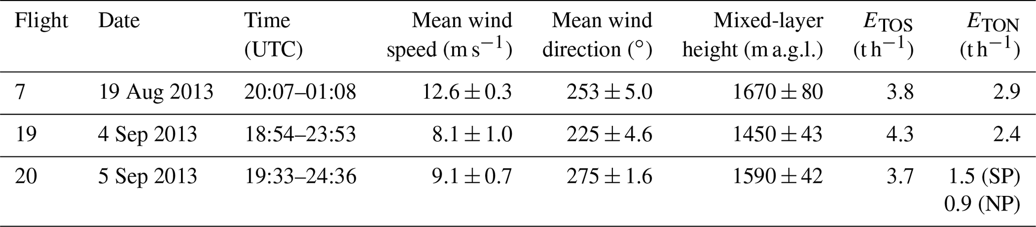
Table 1Average observed meteorological conditions and facility emission rates of TOS (ETOS) and TON (ETON) (determined from extrapolated (to distance = 0) transfer rates; Fig. 1) for TOS and TON during the F7, F19 and F20 flights. SP: southern plume; NP: northern plume.

Changes in the mass transfer rate T (denoted ΔT) in units of t h−1 were then calculated as the differences in T between pairs of virtual screens. The uncertainty in ΔT was estimated as 8 % for TOS and 26 % for TON, as supported by emission rate uncertainties determined for box flights (Gordon et al., 2015). The uncertainty analysis for box flights is applicable to ΔT here, as both account for uncertainties with an upwind and a downwind screen. The ΔT uncertainties were propagated through subsequent calculations.
Knowing the change in mass transfer rate ΔT and accounting for the net rates of chemical loss and formation between screens for SO2 and pSO4, the deposition rates (and subsequently the deposition flux in tonnes S (or N) km−2 h−1, Sect. 2.4) were determined for the sulfur compounds as follows:
where is the rate of chemical reaction loss of sulfur mass in SO2, is the rate of chemical formation of sulfur mass as pSO4, and are deposition rates of sulfur mass in SO2 and pSO4, respectively, and t1 and t2 are plume interception times at Screen 1 and Screen 2, respectively. Note that the chemical loss rate of SO2 is set to be equivalent to the formation rate of pSO4, i.e. = . Equation (4) for TOS can also similarly be written as shown in Eq. (5).
Units in Eqs. (2) to (5) are all in t h−1. Reaction with the OH radical was considered to be the most significant chemical loss of SO2 and the most significant path for the formation of pSO4. and were determined using estimated OH radical concentrations, which were estimated using the methodology described in Supplement Sect. S4. Although TON encompasses a range of different N species with expected differences in their deposition rates, it was not possible to quantitatively separate their chemical formation/losses from their deposition rates with this method. For total oxidized sulfur TOS (i.e. sulfur in SO2 + pSO4) and total oxidized nitrogen TON (i.e. nitrogen in NOy), the chemistry term is not relevant, and thus the dry deposition rate DTOS was directly determined from ΔTTOS using Eq. (4) and, respectively, for TON.
2.4 Dry deposition fluxes and dry deposition velocities
Average dry deposition fluxes (F) for TOS and TON were obtained by dividing the deposition rates D in t h−1 by the footprint surface area of the plume between two adjacent screens (Fig. 1 grey-shaded regions), as shown in Eq. (6) for the dry deposition flux FTOS of TOS (in t S km−2 h−1):
where the surface area, Area, was identified as the geographic area under the plume extending to the edges of the plume where concentrations fell to background levels (i.e. SO2 to ∼0 ppb; SO4 ∼0.2 µg m−3). This approach was similarly used to derive deposition fluxes from an air quality model, Global Environmental Multiscale – Modelling Air-quality and Chemistry (GEM-MaCH) (Moran et al., 2014; also see Supplement Sect. S5 for details). The geographic surface area uncertainty is estimated at 5 %. Dry deposition fluxes between the sources and the first screen were also estimated using change in mass transfer rate ΔT based on the extrapolated transfer rates back to the source region (“extended” region). The surface area boundaries for these “extended” regions were determined using latitude and longitude coordinates that were weighted by emissions. This was done by first using the average wind direction from Screen 1 and creating a set of parallel back trajectories (∼20) starting at different parts of Screen 1 back across the source region. For TON, the NOx emission sources along each back trajectory were weighted by their NOx emissions to obtain an emissions-weighted centre location with latitude and longitude coordinates for each back trajectory. The line connecting these emissions-weighted centre locations formed the boundary of the extended surface area. The extended surface area was similarly determined for TOS based upon the known locations of the major SO2 point sources. The uncertainty of the “extended” regions is estimated at 10 % based on repeated optimizations of the geographical area. Surface areas are visualized as grey-shaded regions between screens in Fig. 1 and tabulated in Supplement Table S1.
Spatially averaged dry deposition velocities, Vd, based on the aircraft measurements were determined over the surface area between screens using average plume concentrations across pairs of screens at about 40 m above the ground for SO2 and TON (e.g. Eq. 7 for SO2 in units of cm s−1). Although TOS includes the S in both SO2 and pSO4, only SO2 is used in the calculation of Vd since the deposition behaviour of gases and particles differs substantially, and particles additionally have size-dependent deposition rates (Emerson et al., 2020). As the dominant form of TOS is SO2 (>92 %), the deposition behaviour of TOS is expected to be largely driven by that of SO2. The measured TON does not include pNO3.
The largest source of uncertainty in Vd calculated this way was the determination of concentration at 40 m above the surface as the measurements were extrapolated from the lowest aircraft altitude to the surface and interpolated concentrations were used. The measurement-derived Vd are compared with those from the air quality model GEM-MACH, which uses inferential methods.
2.5 Monte Carlo simulations of dry deposition velocities using multiple resistance-based parameterizations
Parameterization of dry deposition in inferential algorithms is commonly based on a resistance approach with dry deposition velocity depending on three main resistance terms as below:
where Ra, Rb and Rc represent the aerodynamic, quasi-laminar sublayer and bulk surface resistances, respectively. Although these resistance terms are common among many regional air quality models (Wu et al., 2018), the formulae used (and inputs into these formulae) to calculate the individual resistance terms differ significantly among the inferential deposition algorithms. To assess the potential for a general underestimation of Vd across different inferential deposition algorithms and to compare with the aircraft-derived Vd, five different inferential deposition algorithms, including that used in the GEM-MACH model for calculating Vd (Wu et al., 2018), were incorporated into a Monte Carlo simulation for Vd for SO2. NOy was not considered here, as its measurement includes multiple reactive nitrogen oxide species with different individual deposition velocities. We note that many of the inferential algorithms are based on observations of SO2 and O3 deposition made at single sites, and the extent to which a chemical is similar to SO2 or O3 features in its Vd calculation – the comparison thus has relevance for species aside from SO2. The five deposition algorithms considered are denoted ZHANG, NOAH-GEM, C5DRY, WESLEY and GEM-MACH and are compared in Wu et al. (2018) (except the algorithm in GEM-MACH). The five algorithms all use a big-leaf approach for calculating Vd; i.e. Vd is based on the resistance-analogy approach for calculating dry deposition velocity, where Vd is the reciprocal sum of three resistance terms Ra, Rb and Rc. Although the approach is similar, the formulations of Ra, Rb and Rc between the algorithms are substantially different (Table 1 in Wu et al., 2018). Results from Wu et al. (2018) suggest that the differences in Ra+Rb between different models would cause a difference in their Vd values of the order of 10 %–30 % for most chemical species (including SO2 and NO2), although the differences can be much larger for species with near-zero Rc such as HNO3.
To perform the simulations, formulae for the first four algorithms were taken from Wu et al. (2018) and for GEM-MACH taken from Makar et al. (2018). The stomatal resistance in the ZHANG algorithm was from Zhang et al. (2002). The GEM-MACH formula (Eq. 8.7 in the Supplement of Makar et al., 2018) for mesophyll resistance Rmx contained a typo (missing the Leaf Area Index – LAI) and was corrected for as follows.
Prescribed input values were constrained by the range of possible values consistent with the conditions during the aircraft flights and are shown in Supplement Table S3 with associated references. Calculations for the Ra term were based on unstable and dry conditions as observed during the aircraft flights. The Monte Carlo simulation generated a distribution of possible Vd values, based on randomly generated values of the input variables to each algorithm and selected from Gaussian distributions with a range of 3σ for all input parameters. All simulations were performed with the same input values that were common between the algorithms.
3.1 Meteorological and emissions conditions during the transformation flights
Three aircraft flights, Flights 7 (F7), 19 (F19) and 20 (F20), were conducted in Lagrangian patterns where the same plume emitted from oil sands activities was repeatedly sampled for a 4–5 h period and up to 107–135 km downwind of the AOSR. The first screen of each flight captured the main emissions from the oil sands operations with no additional anthropogenic sources between subsequent screens downwind. The main sources of nitrogen oxides were from exhaust emissions from off-road vehicles used in open pit mining activities and sulfur and nitrogen oxides from the elevated facility stack emissions associated with the desulfurization of raw bitumen (Zhang et al., 2018). As depicted in Fig. 1, F7 and F19 captured a plume that contained both sulfur and nitrogen oxides. The westerly wind direction and orientation of the aircraft tracks on F20 resulted in the measurement of two distinct plumes: one plume exhibited increased levels of sulfur and nitrogen oxides mainly from the facility stacks and the other plume contained elevated levels of nitrogen oxides, mainly from the open pit mining activities, and no SO2.
During the experiments, the dry deposition rates (D) (t h−1) were quantified under different meteorological conditions and emissions levels of TOS and TON (ETOS and ETON) for the three flights (see Table 1). These differences played important roles in the observed pollutant concentrations and resulting dry deposition fluxes for F7, F19 and F20. Mixed-layer heights (MLHs) were derived from aircraft vertical profiles that were conducted in the centre of the plume at each downwind set of transects. The profiles of temperature, dew point temperature, relative humidity and pollutant mixing ratios were inspected for vertical gradients, indicating a contiguous layer connected to the surface. The highest MLH was determined for F7 at 2500 m a.g.l., whereas F19 had the lowest MLH at 1200 m a.g.l. (Table 1). In F20, the MLH was 2100 m a.g.l. The combination of a high MLH in F7 with the highest wind speeds resulted in the lowest pollutant concentrations of the three flights. In F19, lower wind speeds and the lowest mixed-layer heights led to the highest pollutant levels. F20 had emissions and meteorological conditions that were in between F7 and F19, resulting in pollutant concentrations between those of F7 and F19.
Emission rates of SO2 and NOx (designated as ETOS and ETON) from the main sources in the AOSR were estimated from the aircraft measurements and varied significantly between the 3 flight days. The measurement-based emission rates of ETOS and ETON were taken from the mass transfer rates of and (described in Methods) by extrapolating backwards to the source locations in the AOSR using exponential functions (Fig. 2, Sect. 3.2). For TOS, the source location was set at 57.017∘ N, −111.466∘ W, where the main stacks for SO2 emissions are located. For TON, the source locations were determined from geographically weighted locations. Emission rates ETOS and ETON for each flight are shown in Table 1.

Figure 2TERRA-derived transfer rates of (a) TOS and (b) TON for F7, F19 and F20. The vertical bars indicate the propagated uncertainties. The model emission rates ETOS and ETON are shown by the open symbols.
Model-based ETOS and ETON were also obtained from the 2.5 km × 2.5 km gridded emissions fields that were specifically developed for model simulations of the large AOSR surface mining facilities (Zhang et al., 2018), i.e. Suncor Millennium, Syncrude Mildred Lake, Syncrude Aurora North, Shell Canada Muskeg River Mine & Muskeg River Mine Expansion, CNRL Horizon Project and Imperial Kearl Mine. The emissions fields have been used in GEM-MACH (described in Supplement Sect. S5) to carry out a number of model simulations (Zhang et al., 2018; Makar et al., 2018), including for the present study. In this work, emissions were summed from various sources, including off-road, point (continuous emissions monitoring – CEMS), and point (non-CEMS), for the surface mines to obtain total AOSR hourly emission rates for the flight time periods of interest (Table 2). The standard deviations reflect the emissions variations during the simulated flight.
Table 2Model average meteorological conditions and facility emission rates of TOS (ETOS) and TON (ETON) during the F7, F19 and F20 flights as described above. SP: southern plume; NP: northern plume.
3.2 Mass transfer rates
The mass transfer rates T (in t h−1) across the virtual flight screens for all three flights are shown for TOS and TON in Fig. 1 and plotted in Fig. 2. In F20, two distinct TON plumes were observed, allowing separate T calculations for TON. Monotonic decreases in T were observed for both TOS and TON during transport downwind in all flights, clearly showing dry depositional losses. The deposition rate D (Methods, Sect. 2.3) was used to estimate the cumulative deposition of TOS and TON as a fraction of ETOS or ETON and is shown in Fig. 3 for F7, F19 and F20 for transport distances of up to 107–135 km downwind of the sources. Curves were fitted to the TOS and TON dry deposition cumulative percentages from which and τ were determined (Supplement Table S1). The transport e-folding distance () was determined where 63.2 % of ETOS (or ETON) was dry deposited, i.e. . The atmospheric lifetimes (τ) were derived as , where u was the average wind speed across the distance . These estimates were compared with predictions from the regional air quality model GEM-MACH (Makar et al., 2018; Moran et al., 2014; Supplement Sect. S5) using facility emission rates (Table 2). For TOS during F19 (Fig. 3b, e), the observed cumulative deposition at the maximum distance accounted for 74 ± 5 % vs. the modelled 21 % of ETOS. The measurements indicate that the cumulative deposition of TOS was due mostly to SO2 dry deposition, where SO2 was ∼100 % of TOS closest to the oil sands sources, decreasing to 94 % farthest downwind. Although the modelled cumulative deposition of TOS was significantly lower than the observations, the fractional deposition of SO2 was similar, decreasing from ∼100 % to 95 % of TOS. Fitting a curve to D and interpolating the cumulative deposition fraction to the 63.2 % ETOS loss leads to a of 71 ± 1 km vs. 500 km for the model prediction. Under the prevailing wind conditions, the observed distance indicates a τ for TOS of approximately 2.2 h, whereas the model prediction indicated 16 h. Large observation-based values and model prediction differences in lifetime were also evident for the other flights (Supplement Table S1). Clearly, the model predictions significantly underestimated deposition and vastly overestimated and τ. The observation-based values for τ are also lower than average lifetimes of 1–2 d for SO2 and 2–9 d for pSO4 derived from global models (Chin et al., 2000; Benkovitz et al., 2004; Berglen et al., 2004), which include the effects of wet deposition and chemical conversion for SO2, thus making their implicit residence times with respect to dry deposition even longer.
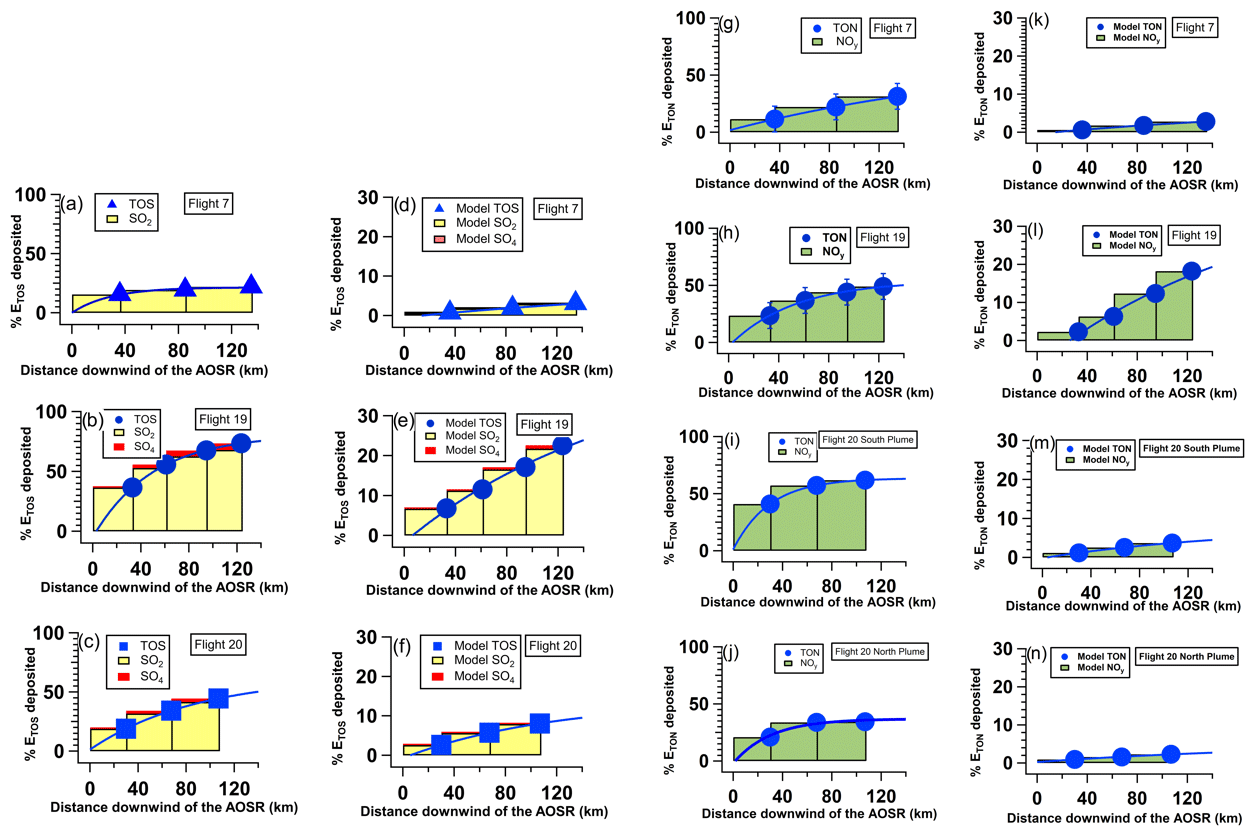
Figure 3Cumulative dry deposition as a percentage of emissions ETOS (a to f) or ETON (g to n) for F7, F19 and F20 measurements with corresponding GEM-MACH model predictions. The bars show the dry deposition due to SO2 and pSO4. The curves were fitted to the TOS and TON dry deposition percentages from which and τ were determined.
For TON in F19 (Fig. 3h, l), the observed cumulative deposition accounted for 49 ± 11 % of ETON at the maximum flight distance vs. 19 % predicted by the model. Similar model underestimates for cumulative deposition fractions were found for F7 and F20. Extrapolating to the 63.2 % cumulative deposition fraction, was estimated to be 190 ± 7 km for F19 vs. a predicted 650 km from the model, implying a τ of approximately 5.6 h for the measurement-based results and 23 h for the model prediction. Again, analogous differences for F7 and F20 were found (Supplement Table S1). Similar to TOS, the measurement-based and τ values for TON were significantly smaller than commonly accepted lifetimes of a few days for nitrogen oxides in the boundary layer (Munger et al., 1998).
3.3 Dry deposition fluxes F
Using the deposition rate D (in tonnes S or N h−1), the average dry deposition fluxes, F (in tonnes S or N km−2 h−1), were calculated by dividing D by the plume footprint surface areas estimated by extending to the plume edges where the concentrations fell to background levels (Methods, Sect. 2.4). These footprints are shown as the grey-shaded geographic areas in Fig. 1, totalling 3500, 5700, and 4200 km2 for the F7, F19, and F20 plumes, respectively; see Supplement Table S1 for TON plume areas). Figure 4a shows FTOS values for all three flights, exhibiting exponential decreases with increasing distance away from the sources and showing e-folding distances for FTOS of 18, 27, and 55 km for F7, F19, and F20, respectively. More than 90 % of the decreases in FTOS were accounted for by . Similarly, FTON decreased exponentially with increasing transport distances in all flights (Fig. 4c), exhibiting e-folding distances of 18 and 33 km for F7 and F19 and 55 and 189 km for the southern and northern TON plumes during F20, respectively. These e-folding distances were similar to those for FTOS, indicating similar rates of decreases in FTON with transport distances.
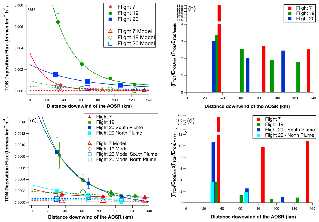
Figure 4Dry deposition fluxes FTOS and FTON (in t km−2 h−1) determined from measurements (solid symbols) and GEM-MACH model predictions (open symbols). (a) FTOS, (b) ratios of measurement-to-model normalized emissions , (c) FTON, and (d) ratios of measurement-to-model normalized emissions .
The potential for other processes to contribute to the derived TOS and TON fluxes were considered, including losses from the boundary layer to the free troposphere and re-emission of TOS or TON species from the surface back to the gas phase. Two different approaches, a finite-jump model and a gradient flux approach (Stull, 1988; Degrazia et al., 2015), were used to estimate the potential upward loss across the interface between the boundary layer and the free troposphere for sulfur and nitrogen. In both approaches, the upward S flux was a minor loss at <45 g km−2 h−1, about 3 orders of magnitude lower than the several to many kg km−2 h−1 horizontal advectional transport that was determined using TERRA. For N, the upward flux was estimated to be ∼570 g km−2 h−1, so although a larger flux than S, it is about factor of 18 lower than the TON fluxes derived from observations.
As expected from the τ and transport e-folding distance comparisons, the GEM-MACH model FTOS was significantly lower than the measurement-based FTOS results (Fig. 4a), with the model FTOS e-folding distances usually large: 133, 797, and 57 km for F7, F19, and F20, respectively, or 7.4, 29.5, and 1.1 times longer than the corresponding measurement results. Part of the differences between model and measurement FTOS could be explained by differences in actual vs. model emissions, ETOS (Tables 1 vs. 2). To remove the influence of emissions, an emission-normalized flux (= and ) was calculated for both measurement and model (Supplement Fig. S2). Figure 4b shows the ratios of measurement-to-model normalized emissions for TOS. The model emission-normalized fluxes were lower than the measurement-based values by factors of 2.5–14, 1.8–3.4, and 2.0–3.0 for F7, F19, and F20, respectively, decreasing with increased transport distances. However, they coalesce to a factor of 2 at the furthest distances sampled by the aircraft, indicating that the model FTOS estimates were biased low by similar factors. The decreasing trends suggest that at distances further downwind, model fluxes may exceed measurement-based fluxes, albeit at magnitudes lower than those shown in Fig. 4a, which is consistent with earlier study results (Makar et al., 2018). For FTON, the model-predicted values were also lower than the measurement results, especially near the sources (Fig. 4c), and showed little variation with transport distances from the oil sands sources for all flights, in strong contrast to the exponential decays observed from the aircraft. However, the emission-normalized fluxes (= ) for the model approached those from measurements within maximum flying distances for F19 and F20, although still significantly lower for F7 (>10×) (Fig. 4d).
3.4 Dry deposition velocities Vd
The shorter and τ and larger deposition fluxes F near the sources determined from the aircraft measurements compared to predictions by the GEM-MACH model indicate that the model dry deposition velocities Vd were underestimated. Gas-phase Vd in the model is predicted with a standard inferential “resistance” algorithm (Wesley, 1989; Jarvis, 1976), with resistance to deposition calculated for multiple parameters, including aerodynamic, quasi-laminar sublayer and bulk surface resistances (Baldocchi et al., 1987). To demonstrate the model underestimation in Vd, comparisons between the measurement-based and model Vd were made where an evaluation of Vd for TOS and TON was possible. All were converted into by dividing by interpolated SO2 concentrations at 40 m above ground, averaging 1.2 ± 0.5, 2.4 ± 0.4, and 3.4 ± 0.6 cm s−1 for F7, F19, and F20, respectively, across the plume footprints (Methods Sect. 2.4 and Supplement Table S2). The corresponding model derived in the same way as the observations was 0.72, 0.63, and 0.58 cm s−1, 1.7–5.4 times lower than observations (Supplement Sect. S5; Supplement Table S2). Interestingly, the median Vd for SO2 of 4.1 cm s−1 determined using eddy covariance/vertical gradient measurements from a tower in the AOSR is higher than the mass-balanced method, showing an even larger discrepancy compared to the model (Supplement Sect. S3; Fig. S5). Similarly, derived Vd−TON averaged 2.8 ± 0.8, 1.6 ± 0.5, 4.7 ± 1.4, and 2.2 ± 0.7 cm s−1 for the F7, F19, and F20 southern plumes and F20 northern plume, respectively (Supplement Table S2), 1.2–5.2 times higher than the corresponding modelled Vd−TON of 1.4, 1.3, 0.92, and 0.90 cm s−1.
Using the observations, it was not possible to derive individual TON deposition rates separate from their chemical formation/losses. In previous modelling work, Makar et al. (2018) use the GEM-MACH model and describe the relative contributions of different TOS and TON species towards total S and N deposition in the AOSR. TON was dominated by dry NO2 (g) dry deposition fluxes close to the sources (>70 % of total N close to the sources), and dry HNO3 (g) dry deposition increases with increasing distance from the sources (remaining <30 % of total N) and other sources of TON having minor contributions to deposition (<10 %). Although TON encompasses a range of different N species with expected differences in their deposition rates, comparisons of Vd−TON with the model show, nevertheless, that overall large differences do exist.
3.5 Monte Carlo simulations of Vd for SO2
To further demonstrate observation–model differences, Vd distributions of SO2 from five common inferential dry deposition algorithms (Wu et al., 2018; Makar et al., 2018) were determined for the conditions encountered during the flights using a Monte Carlo approach as described in Methods Sect. 2.5. Results for the Vd simulation algorithms are shown in Fig. 5a. Histograms for all five algorithms have peak Vd values at ∼1 cm s−1 or lower. Probability distributions for the individual resistance terms Ra, Rb, and Rc showed that the dominant resistance driving Vd was the Rc term (Supplement Fig. S3). Also shown in Fig. 5a are the measurement-derived Vd for Flights 7, 19 and 20 and that from the Oski-ôtin ground site. The observed Vd values are larger than the Vd values for most of the simulations, with the exception of Flight 7, where the Zhang et al. (2002), NOAH-GEM (Wu et al., 2018) and C5DRY (Wu et al., 2018) algorithms' distributions agree with the observations. All algorithms are biased low relative to the observations for the remaining flights and the Oski-ôtin ground site. It is noted that the ground-site observations that were derived using a standard flux tower methodology (Supplement Sect. S3) at a single site appeared to be higher than all other Vd; nevertheless, these observations are closer to the aircraft values than the algorithm estimates. These results indicate that an underestimation of Vd relative to both aircraft and ground-based measurements in the AOSR is not unique to the GEM-MACH model or its dry deposition algorithm; similar results would occur with the other algorithms included in the Monte Carlo simulations, all of which are used within other regional models.
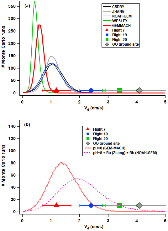
Figure 5(a) Distributions of Vd for SO2 from Monte Carlo simulations using five different deposition parameterizations (Wu et al., 2018; Makar et al., 2018) and (b) Monte Carlo simulations for the GEM-MACH algorithm using a pH = 8 and using a pH = 8 plus replacing the GEM-MACH algorithm Ra and Rb formulae with that from Zhang et al. (2002) and NOAH-GEM (Wu et al., 2018), respectively. Aircraft-derived Vd for F7, F19 and F20 as well as the median value for the Oski-ôtin ground site (Supplement Fig. S5) are shown in both (a) and (b) for comparison.
To investigate the possible reasons behind the low model Vd relative to the observations, a series of sensitivity tests using SO2 were conducted. Differences in model Vd have been shown to be mainly due to differences in the calculated Rc (Wu et al., 2018), and sensitivity tests here indicated that Rc is particularly sensitive to the cuticular resistance Rcut. Hence, factors causing Rcut to change can have significant impact on model Vd. In some of the algorithms, Rcut and other resistance terms are dependent on the effective Henry's law constant for SO2. The Monte Carlo simulations for Fig. 5 assumed a surface pH = 6.68 resulting in a of 1 × 10⁵ for SO2. Additional Monte Carlo simulations were performed for the GEM-MACH dry deposition algorithm by adjusting assuming different pH with small variations from a pH = 6.68 significantly changing Rc, Rcut, and Vd (Supplement Fig. S4). In Fig. 5b – red dashed line – with a surface pH change from 6.68 to 8, consistent with possible alkaline surfaces in the AOSR (Makar et al., 2018), in the GEM-MACH simulation, the Vd distribution is moved to larger values, with its peak value shifting from 0.6 to 1.4 cm s−1. These results show that model Vd may be highly sensitive to assumed surface pH, at least when using some inferential dry deposition algorithms which are pH-dependent. However, Fig. 5b shows that this pH-associated increase in Vd is still insufficient to encompass the range of measurement-derived Vd. Increasing pH to 8 for the GEM-MACH simulation reduces Rcut, hence Rc, to values much smaller than Ra and Rb, suggesting that model Vd cannot further increase without reductions in both Ra and Rb. In other words, Ra and Rb were probably overestimated in the current deposition velocity algorithms. By using the Zhang et al. (2002) Ra and the NOAH-GEM (Wu et al., 2018) Rb parameterizations in the GEM-MACH algorithm, a further shift of the GEM-MACH Vd distribution to larger values was found, with the range encompassing most of the observations (Fig. 5b, pink dashed line). Using the Zhang and NOAH-GEM parameterizations, rather than the GEM-MACH parameterization, would decrease the Ra and Rb for the momentum, heat and moisture fluxes as well but still remain within the range of what is expected based on published parameterizations (Wu et al., 2018, and references therein).
The potential for re-emission of TOS and TON species was also considered. Fulgham et al. (2020) report that the bidirectional fluxes of volatile organic acids are driven by an equilibrium partitioning between surface wetness and the atmosphere. The observations presented here represent the net flux of all processes including the effects of deposition and any potential re-emissions of TOS and TON compounds should this process occur. As the results show a net downward flux (i.e. net deposition), if any re-emission was occurring, it would be smaller than the deposition fluxes observed here, which are themselves higher than shown by currently available deposition algorithms. This implies that the deposition part of the flux must be even larger than the net observed flux, and the measured net fluxes presented here should then be considered minimum values. The current deposition algorithms do not include bidirectional fluxes for inorganics, and adjustments related to pH in some situations may not be sufficient to parameterize deposition fluxes. A bidirectional approach may be needed that would include not only [H+], but also surface heterogeneous reactions, to determine near-surface equilibrium concentrations of co-depositing gases such as ammonia and nitric acid.
It is clear that from the Monte Carlo simulations for SO2 Vd comparisons, inferential dry deposition algorithms as used in regional and global chemical transport models need to be further validated and improved, especially over large geographic regions. Here, the role of pH was identified for improvement in some algorithms along with possible improvement in aerodynamic and quasi-laminar sublayer resistance parameters. Yet for other algorithms and for TON compounds, the model low biases in Vd remain to be investigated.
The underestimates suggest that the applications of these algorithms in regional or global models may significantly underestimate predictions of TOS dry depositional loss from the atmosphere. Underestimates in Vd are the result of a combination of uncertainties in the parameterizations of each algorithm. In the case of the algorithm used in GEM-MACH, by adjusting the assumed surface pH from 6.68 to 8 (justifiable given the considerable dust emissions in the region: Zhang et al., 2018), the model Vd moved closer to the aircraft-derived values (Fig. 5b), reducing the model–observation gap by approximately two-thirds. In addition, substituting the aerodynamic resistance and quasi-laminar sublayer resistance parameterizations in the GEM-MACH algorithm with that from Zhang et al. (2002) and NOAH-GEM (Wu et al., 2018), respectively, resulted in a further increase in the model Vd distribution that encompasses most of the observations (Fig. 5b). Clearly, different algorithms respond differently to changes in the parameterizations, and validation and adjustment to each algorithm need measurement-based results over large regions such as derived here.
The atmospheric transport distances and lifetimes and τ determined from the aircraft measurements are substantially shorter than the GEM-MACH model predictions, and the dry deposition fluxes F and velocities and Vd near sources are larger compared to the predictions by GEM-MACH and five inferential dry deposition velocity algorithms, respectively. There are important implications for these measurement–model discrepancies. Such discrepancies indicate that regional or global chemical transport models using these algorithms are biased low for local deposition and high for long-range transport and deposition, and TOS and TON losses from the atmosphere are significantly underpredicted, resulting in overestimated lifetimes. While the measurements took place over a relatively short time period, these results indicate that TOS and TON may be removed from the atmosphere at about twice the rate as predicted by current atmospheric deposition algorithms. This, in turn, implies a potentially significant impact on deposition over longer timescales (potentially weeks to months) and relevance towards cumulative environmental exposure metrics such as critical loads and their exceedance. A faster near-source deposition velocity for emitted reactive gases may imply less S and N mass being available for long-range transport, reducing concentrations and deposition further downwind. The near-source higher deposition velocity thus has the important implication of a reduction in more distant and longer timescale deposition for locations further from the sources. Moreover, emissions assessed through network measurements or budget analysis of atmospheric TOS and TON (Sickles and Shadwick, 2015; Paulot et al., 2018; Berglen et al., 2004) may be underestimated due to lower Vd used in these estimates and may require reassessment of the effectiveness of control policies. Shorter τ for TOS and TON reduces their atmospheric spatial scale and intensity of smog episodes, potentially reducing human exposures (Moran et al., 2014). Importantly, shorter τ for TOS and TON reduces their contribution to atmospheric aerosols; consequently, the negative direct and indirect radiative forcing from these sulfur and nitrogen aerosols is reduced, reducing their cooling effects on climate (Solomon et al., 2007). These impacts suggest that more measurements to determine τ and F for these pollutants across large geographic scales and different surface types are necessary for better quantifying their climate and environmental impacts in support of policy. While in the past such determination was difficult and/or impossible, the present study provides a viable methodology to achieve such a goal.
All the computer code associated with the TERRA algorithm, including for the kriging of pollutant data, a demonstration dataset and associated documentation are freely available upon request. The authors request that future publications which make use of the TERRA algorithm cite this paper, Gordon et al. (2015), Liggio et al. (2016), or Li et al. (2017) as appropriate.
All data used in this publication are freely available on the Canada-Alberta Oil Sands Environmental Monitoring Information Portal: https://www.canada.ca/en/environment-climate-change/services/oil-sands-monitoring/monitoring-air-quality-alberta-oil-sands.html (Government of Canada, 2019).
The supplement related to this article is available online at: https://doi.org/10.5194/acp-21-8377-2021-supplement.
KH, SML, JL, SGM, RM, RMS, JO'B and MW all contributed to the collection of aircraft observations in the field. KH, RM and JO'B made the SO2, NOy and pSO4 measurements and carried out subsequent QA/QC of data. RM analysed canister VOCs and provided OH concentration estimates. RMS made and provided the ground-site deposition velocity measurements. AD contributed to the development of TERRA. JL wrote the Monte Carlo code. PM and AA ran the model and provided model analyses. JZ provided emissions data. LZ and RMS provided deposition algorithm parameters. KH and SML wrote the paper input from all the co-authors.
The authors declare that they have no conflict of interest.
The authors thank the National Research Council of Canada flight crew of the Convair-580, the Air Quality Research Division technical support staff, Julie Narayan for in-field data management support, and Stewart Cober for the management of the study.
The project was funded by the Air Quality program of Environment and Climate Change Canada and the Oil Sands Monitoring (OSM) program. It is independent of any position of the OSM program.
This paper was edited by Barbara Ervens and reviewed by two anonymous referees.
Aubinet, M., Vesala, T., and Papale, D. (Eds.): Eddy Covariance, Springer Atmospheric Sciences, Springer, Dordrecht, The Netherlands, 2012.
Baldocchi, D. D., Vogel, C. A., and Hall, B.: A canopy stomatal resistance model for gaseous deposition to vegetated surfaces, Atmos. Environ., 21, 91–101, https://doi.org/10.1016/0004-6981(87)90274-5, 1987.
Baray, S., Darlington, A., Gordon, M., Hayden, K. L., Leithead, A., Li, S.-M., Liu, P. S. K., Mittermeier, R. L., Moussa, S. G., O'Brien, J., Staebler, R., Wolde, M., Worthy, D., and McLaren, R.: Quantification of methane sources in the Athabasca Oil Sands Region of Alberta by aircraft mass balance, Atmos. Chem. Phys., 18, 7361–7378, https://doi.org/10.5194/acp-18-7361-2018, 2018.
Benkovitz, C. M., Schwartz, S. E., Jensen, M. P., Miller, M. A., Easter, R. C., and Bates, T. S.: Modeling atmospheric sulfur over the Northern Hemisphere during the Aerosol Characterization Experiment 2 experimental period, J. Geophys. Res.-Atmos., 109, D22207, https://doi.org/10.1029/2004JD004939, 2004.
Berglen, T. F., Berntsen, T. K., Isaksen, I. S. A., and Sundet, J. K.: A global model of the coupled sulfur/oxidant chemistry in the troposphere: The sulfur cycle, J. Geophys. Res.-Atmos., 109, D19310, https://doi.org/10.1029/2003JD003948, 2004.
Bobbink, R., Hicks, K., Galloway, J., Spranger, T., Alkemade, R., Ashmore, M., Bustamante, M., Cinderby, S., Davidson, E., Dentener, F., Emmett, B., Erisman, J.-W., Fenn, M., Gilliam, F., Nordin, A., Pardo, L., and De Vries, W.: Global assessment of nitrogen deposition effects on terrestrial plant diversity: a synthesis, Ecol. Appl, 20, 30–59, https://doi.org/10.1890/08-1140.1, 2010.
Brook, J. R., Di-Giovanni, F., Cakmak, S., and Meyers, T. P.: Estimation of dry deposition velocity using inferential models and site-specific meteorology – uncertainty due to siting of meteorological towers, Atmos. Environ., 31, 3911–3919, https://doi.org/10.1016/S1352-2310(97)00247-1, 1997.
Chin, M., Savoie, D. L., Huebert, J., Bandy, A. R., Thornton, D. C., Bates, T. S., Quinn, P. K., Saltzman, E. S., and De Bruyn, W. J.: Atmospheric sulfur cycle simulated in the global model GOCART: Comparison with field observations and regional budgets, J. Geophys. Res.-Atmos., 105, 24689–24712, https://doi.org/10.1029/2000JD900384, 2000.
Christian, G., Ammann, M., D'Anna, B., Donaldson, D. J., and Nizkorodov, S. A.: Heterogeneous photochemistry in the atmosphere, Chem. Rev., 115, 4218–4258, https://doi.org/10.1021/cr500648z, 2015.
DeCarlo, P. F., Kimmel, J. R., Trimborn, A., Northway, M. J., Jayne, J. T., Aiken, A. C., Gonin, M., Fuhrer, K., Horvath, T., Docherty, K. S., Worsnop, D. R., and Jimenez, J. L.: Field-deployable, high-resolution, time-of-flight aerosol mass spectrometer, Anal. Chem., 78, 8281–9289, https://doi.org/10.1021/ac061249n, 2006.
de Gouw, J. and Warneke, C.: Measurements of volatile organic compounds in the earth's atmosphere using proton-transfer-reaction mass spectrometry, Mass Spectrom. Rev., 26, 223–257, https://doi.org/10.1002/mas.20119, 2007.
Degrazia, G. A., Maldaner, S., Buske, D., Rizza, U., Buligon, L., Cardoso, V., Roberti, D. R., Acevedo, O., Rolim, S. B. A., and Stefanello, M. B.: Eddy diffusivities for the convective boundary layer derived from LES spectral data, Atmos. Pollut. Res., 6, 605–611, https://doi.org/10.5094/APR.2015.068, 2015.
Dentener, F., Drevet, J., Lamarque, J. F., Bey, I., Eickhout, B., Fiore, A. M., Hauglustaine, D., Horowitz, L. W., Krol, M., Kulshrestha, U. C., Lawrence, M., Galy-Lacaux, C., Rast, S., Shindell, D., Stevenson, D., Van Noije, T., Atherton, C., Bell, N., Bergman, D., Butler, T., Cofala, J., Collins, B., Doherty, R., Ellingsen, K., Galloway, J., Gauss, M., Montanaro, V., Müller, J. F., Pitari, G., Rodriguez, J., Sanderson, M., Solmon, F., Strahan, S., Schultz, M., Sudo, K., Szopa, S., and Wild, O.: Nitrogen and sulfur deposition on regional and global scales: A multimodel evaluation, Global Biogeochem. Cy., 20, GB4003, https://doi.org/10.1029/2005GB002672, 2006.
Doney, S. C.: The growing human footprint on coastal and open-ocean biogeochemistry, Science, 328, 1512–1516, https://doi.org/10.1126/science.1185198, 2010.
Dunlea, E. J., Herndon, S. C., Nelson, D. D., Volkamer, R. M., San Martini, F., Sheehy, P. M., Zahniser, M. S., Shorter, J. H., Wormhoudt, J. C., Lamb, B. K., Allwine, E. J., Gaffney, J. S., Marley, N. A., Grutter, M., Marquez, C., Blanco, S., Cardenas, B., Retama, A., Ramos Villegas, C. R., Kolb, C. E., Molina, L. T., and Molina, M. J.: Evaluation of nitrogen dioxide chemiluminescence monitors in a polluted urban environment, Atmos. Chem. Phys., 7, 2691–2704, https://doi.org/10.5194/acp-7-2691-2007, 2007.
Emerson, E. W., Hodshire, A. L., DeBolt, H. M., Bilsback, K. R., Pierce, J. R., McMeeking, G. R., and Farmer, D. K., Revisiting particle dry deposition and its role in radiative effect estimates, P. Natl. Acad. Sci. USA, 117, 26076–26082, https://doi.org/10.1073/pnas.2014761117, 2020.
Finkelstein, P. L., Ellestad, T. G., Clarke, J. F., Meyers, T. P., Schwede, D. B., Hebert, E. O., and Neal, J. A.: Ozone and sulfur dioxide dry deposition to forests: Observations and model evaluation, J. Geophys. Res.-Atmos., 105, 15365–15377, https://doi.org/10.1029/2000JD900185, 2000.
Fowler, D., Pilegaard, K., Sutton, M. A., Ambus, P., Raivonen, M., Duyzer, J., Simpson, D., Fagerli, H., Fuzzi, S., Schjoerring, J. K., Granier, C., Neftel, A., Isaksen, I. S. A., Laj, P., Maione, M., Monks, P. S., Burkhardt, J., Daemmgen, U., Neirynck, J., Personne, E., Wichink-Kruit, R., Butterbach-Bahl, K., Flechard, C., Tuovinen, J. P., Coyle, M., Gerosa, G., Loubet, B., Altimir, N., Gruenhage, L., Ammann, C., Cieslik, S. Paoletti, E., Mikkelsen, T. N., Ro-Poulsen, H., Cellier, P., Cape, J. N., Horváth, L., Loreto, F., Niinemets, Ü., Palmer, P. I., Rinne, J., Misztal, P., Nemitz, E., Nilsoon, D., Pryor, S., Gallagher, M. W., Vesala, T., Skiba, U., Brüggemann, N., Zechmeister-Boltenstern, S., Williams, J., O'Dowd, C. O., Facchini, M. C., de Leeuw, G., Flossman, A., Chaumerliac, N., and Erisman, J. W.: Atmospheric composition change: ecosystems-atmosphere interactions, Atmos. Environ., 43, 5193–5267, https://doi.org/10.1016/j.atmosenv.2009.07.068, 2009.
Fulgham, S. R., Millet, D. B., Alwe, H. D., Goldstein, A. H., Schobesberger, S., and Farmer, D. K.: Surface wetness as an unexpected control on forest exchange of volatile organic acids, Geophys. Res. Lett., 47, e2020GL088745, https://doi.org/10.1029/2020GL088745, 2020.
Gordon, M., Li, S.-M., Staebler, R., Darlington, A., Hayden, K., O'Brien, J., and Wolde, M.: Determining air pollutant emission rates based on mass balance using airborne measurement data over the Alberta oil sands operations, Atmos. Meas. Tech., 8, 3745–3765, https://doi.org/10.5194/amt-8-3745-2015, 2015.
Government of Canada: Monitoring air quality in Alberta oil sands, available at: https://www.canada.ca/en/environment-climate-change/services/oil-sands-monitoring/monitoring-air-quality-alberta-oil-sands.html, (last access: 31 May 2021), 2019.
Howarth, R. W.: Review: coastal nitrogen pollution: a review of sources and trends globally and regionally, Harmful Algae, 8, 14–20, https://doi.org/10.1016/j.hal.2008.08.015, 2008.
Jarvis, P. G.: The interpretation of the variations in leaf water potential and stomatal conductance found in canopies in the field, Philos. T. Roy. Soc. B, 273, 593–610, https://doi.org/10.1098/rstb.1976.0035, 1976.
Li, S.-M., Leithead, A., Moussa, S. G., Liggio, J., Moran, M. D., Wang, D., Hayden, K., Darlington, A., Gordon, M., Staebler, R., Makar, P. A., Stroud, C. A., McLaren, R., Liu, P. S. K., O'Brien, J., Mittermeier, R. L., Zhang, J., Marson, G., Cober, S. G., Wolde, M., and Wentzell, J. J. B.: Differences between measured and reported volatile organic compound emissions from oil sands facilities in Alberta, Canada, P. Natl. Acad. Sci. USA, 114, 3756–3765, https://doi.org/10.1073/pnas.1617862114, 2017.
Liggio, J., Li, S.-M., Hayden, K., Taha, Y. M., Stroud, C., Darlington, A., Drollette, B. D., Gordon, M., Lee, P., Liu, P., Leithead, A., Moussa, S. G., Wang, D., O'Brien, J., Mittermeier, R. L., Brook, J. R., Lu, G., Staebler, R. M., Han, Y., Tokarek, T. W., Osthoff, H. D., Makar, P. A., Zhang, J., Plata, D. L., and Gentner, D. R.: Oil sands operations as a large source of secondary organic aerosols, Nature, 534, 91–94, https://doi.org/10.1038/nature17646, 2016.
Liggio, J., Li, S.-M., Staebler, R. M., Hayden, K., Darlington, A., Mittermeier, R. L., O'Brien, J., McLaren, R., Wolde, M., Worthy, D., and Vogel, F.: Measured Canadian oil sands CO2 emissions are higher than estimates made using internationally recommended methods, Nat. Commun., 10, 1863, https://doi.org/10.1038/s41467-019-09714-9, 2019.
Makar, P. A., Akingunola, A., Aherne, J., Cole, A. S., Aklilu, Y.-A., Zhang, J., Wong, I., Hayden, K., Li, S.-M., Kirk, J., Scott, K., Moran, M. D., Robichaud, A., Cathcart, H., Baratzedah, P., Pabla, B., Cheung, P., Zheng, Q., and Jeffries, D. S.: Estimates of exceedances of critical loads for acidifying deposition in Alberta and Saskatchewan, Atmos. Chem. Phys., 18, 9897–9927, https://doi.org/10.5194/acp-18-9897-2018, 2018.
Matsuda, K., Watanabe, I., Wingpud, V., and Theramongkol, P.: Deposition velocity of O3 and SO2 in the dry and wet season above a tropical forest in northern Thailand, Atmos. Environ., 40, 7557–7564, https://doi.org/10.1016/j.atmosenv.2006.07.003, 2006.
Meyers, T. P., Hicks, B. B., Hosker Jr., R. P., Womack, J. D., and Satterfield, L. C.: Dry deposition inferential measurement techniques, II. Seasonal and annual deposition rates of sulfur and nitrate, Atmos. Environ., 25, 2631–2370, https://doi.org/10.1016/0960-1686(91)90110-S, 1991.
Moran, M. D., Ménard, S., Pavlovic, R., Anselmo, D., Antonopoulos, S., Makar, P. A., Gong, W., Gravel, S., Stroud, C., Zhang, J., Zheng, Q., Robichaud, A., Landry, H., Beaulieu, P.-A., Gilbert, S., Chen, J., and Kallaur, A.: Recent Advances in Canada's National Operational AQ Forecasting System, in: Air Pollution Modeling and its Application XXII. NATO Science for Peace and Security Series C: Environmental Security, edited by: Steyn, D., Builtjes, P., and Timmermans, R., Springer, Dordrecht, the Netherlands, https://doi.org/10.1007/978-94-007-5577-2_37, 2014.
Munger, J. W., Fan, S., Bakwin, P. S., Goulden, M. L., Goldstein, A. H., Colman, A. S., and Wolfsy, S. C.: Regional budgets for nitrogen oxides from continental sources: Variations of rates for oxidation and deposition with season and distance from source regions, J. Geophys. Res.-Atmos., 103, 8355–8368, https://doi.org/10.1029/98JD00168, 1998.
Paulot, F., Malyshev, S., Nguyen, T., Crounse, J. D., Shevliakova, E., and Horowitz, L. W.: Representing sub-grid scale variations in nitrogen deposition associated with land use in a global Earth system model: implications for present and future nitrogen deposition fluxes over North America, Atmos. Chem. Phys., 18, 17963–17978, https://doi.org/10.5194/acp-18-17963-2018, 2018.
Samset, B. H., Myhre, G., Herber, A., Kondo, Y., Li, S.-M., Moteki, N., Koike, M., Oshima, N., Schwarz, J. P., Balkanski, Y., Bauer, S. E., Bellouin, N., Berntsen, T. K., Bian, H., Chin, M., Diehl, T., Easter, R. C., Ghan, S. J., Iversen, T., Kirkevåg, A., Lamarque, J.-F., Lin, G., Liu, X., Penner, J. E., Schulz, M., Seland, Ø., Skeie, R. B., Stier, P., Takemura, T., Tsigaridis, K., and Zhang, K.: Modelled black carbon radiative forcing and atmospheric lifetime in AeroCom Phase II constrained by aircraft observations, Atmos. Chem. Phys., 14, 12465–12477, https://doi.org/10.5194/acp-14-12465-2014, 2014.
Sickles II, J. E. and Shadwick, D. S.: Air quality and atmospheric deposition in the eastern US: 20 years of change, Atmos. Chem. Phys., 15, 173–197, https://doi.org/10.5194/acp-15-173-2015, 2015.
Solomon, S., Qin, D., Manning, M., Chen, Z., Marquis, M., Averyt, K. B., Tignor, M., and Miller, H. L. (eds.): Climate Change 2007: The Physical Science Basis, Contribution of Working Group I to the Fourth Assessment Report of the Intergovernmental Panel on Climate Change, Cambridge University Press, Cambridge, UK, ISBN 978-0-521-88009-1 (pb: 978-0-521-70596-7), 2007.
Stull, R.: An Introduction to Boundary Layer Meteorology, Kluwer Academic Publication, Dordrecht, the Netherlands, https://doi.org/10.1007/978-94-009-3027-8, 666 pp., 1988.
Vet, R., Artz, R. S., Carou, S., Shaw, M., Ro, C.-U., Aas, W., Baker, A., Bowersox, V. C., Dentener, F., Galy-Lacaux, C., Hou, A., Pienaar, J., Gillett, R., Forti, M. C., Gromov, S., Hara, H., Khodzher, T., Mahowald, N. M., Nickovic, S., Rao, P. S. P., and Reid, N. W.: A global assessment of precipitation chemistry and deposition of sulfur, nitrogen, sea salt, base cations, organic acids, acidity and pH, and phosphorus, Atmos. Environ., 93, 3–100, https://doi.org/10.1016/j.atmosenv.2013.10.060, 2014.
Wesley, M. L.: Parameterization of surface resistances to gaseous dry deposition in regional-scale numerical models, Atmos. Environ., 23, 1293–1304, https://doi.org/10.1016/0004-6981(89)90153-4, 1989.
Wesley, M. L. and Hicks, B. B.: A review of the current status of knowledge on dry deposition, Atmos. Environ., 34, 2261–2282, https://doi.org/10.1016/S1352-2310(99)00467-7, 2000.
World Health Organization (WHO): Ambient air pollution: a global assessment of exposure and burden of disease, World Health Organization, available at: https://apps.who.int/iris/handle/10665/250141 (last access: 31 May 2021), 121 p., ISBN 978-9-2415-1135-3, 2016.
Williams, E. J., Baumann, K., Roberts, J. M., Bertman, S. B., Norton, R. B., Fehsenfeld, F. C., Springston, S. R., Nennermacker, L. J., Newman, L., Olszyna, K., Meagher, J., Hartsell, B., Edgerton, E., Pearson, J. R., and Rodgers, M. O.: Intercomparisons of ground-based NOy measurement techniques, J. Geophys. Res.-Atmos., 103, 22261–22280, https://doi.org/10.1029/98JD00074, 1998.
Wright, L. P., Zhang, L., Cheng, I., and Aherne, J.: Impacts and effects indicators of atmospheric deposition of major pollutants to various ecosystems – a review, Aerosol Air Qual. Res., 18, 1953–1992, https://doi.org/10.4209/aaqr.2018.03.0107, 2018.
Wu, Z., Schwede, D. B., Vet, R., Walker, J. T., Shaw, M., Staebler, R., and Zhang, L.: Evaluation and intercomparison of five North American dry deposition algorithms at a mixed forest site, J. Adv. Model. Earth Sy., 10, 1571–1586, https://doi.org/10.1029/2017MS001231, 2018.
Zhang, J., Moran, M. D., Zheng, Q., Makar, P. A., Baratzadeh, P., Marson, G., Liu, P., and Li, S.-M.: Emissions preparation and analysis for multiscale air quality modeling over the Athabasca Oil Sands Region of Alberta, Canada, Atmos. Chem. Phys., 18, 10459–10481, https://doi.org/10.5194/acp-18-10459-2018, 2018.
Zhang, L., Moran, M. D., Makar, P., and Brook, J. R.: Modelling gaseous dry deposition in AURAMS: a unified regional air-quality modelling system, Atmos. Environ., 36, 537–560, 2002.