Wintertime direct radiative effects due to black carbon (BC) over the Indo-Gangetic Plain as modelled with new BC emission inventories in CHIMERE

To reduce the uncertainty in climatic impacts induced by black carbon (BC) from global and regional aerosol–climate model simulations, it is a foremost requirement to improve the prediction of modelled BC distribution, specifically over the regions where the atmosphere is loaded with a large amount of BC, e.g. the Indo-Gangetic Plain (IGP) in the Indian subcontinent. Here we examine the wintertime direct radiative perturbation due to BC with an efficiently modelled BC distribution over the IGP in a high-resolution (0.1^∘ × 0.1^∘) chemical transport model, CHIMERE, implementing new BC emission inventories. The model efficiency in simulating the observed BC distribution was assessed by executing five simulations: Constrained and bottomup (bottomup includes Smog, Cmip, Edgar, and Pku). These simulations respectively implement the recently estimated India-based observationally constrained BC emissions (Constrained_emiss) and the latest bottom-up BC emissions (India-based: Smog-India; global: Coupled Model Intercomparison Project phase 6 – CMIP6, Emission Database for Global Atmospheric Research-V4 – EDGAR-V4, and Peking University BC Inventory – PKU). The mean BC emission flux from the five BC emission inventory databases was found to be considerably high (450–1000 kg km⁻² yr⁻¹) over most of the IGP, with this being the highest (> 2500 kg km⁻² yr⁻¹) over megacities (Kolkata and Delhi). A low estimated value of the normalised mean bias (NMB) and root mean square error (RMSE) from the Constrained estimated BC concentration (NMB: < 17 %) and aerosol optical depth due to BC (BC-AOD) (NMB: 11 %) indicated that simulations with Constrained_emiss BC emissions in CHIMERE could simulate the distribution of BC pollution over the IGP more efficiently than with bottom-up emissions. The high BC pollution covering the IGP region comprised a wintertime all-day (daytime) mean BC concentration and BC-AOD respectively in the range 14–25 µg m⁻³ (6–8 µg m⁻³) and 0.04–0.08 from the Constrained simulation. The simulated BC concentration and BC-AOD were inferred to be primarily sensitive to the change in BC emission strength over most of the IGP (including the megacity of Kolkata), but also to the transport of BC aerosols over megacity Delhi. Five main hotspot locations were identified in and around Delhi (northern IGP), Prayagraj–Allahabad–Varanasi (central IGP), Patna–Palamu (mideastern IGP), and Kolkata (eastern IGP). The wintertime direct radiative perturbation due to BC aerosols from the Constrained simulation estimated the atmospheric radiative warming (+30 to +50 W m⁻²) to be about 50 %–70 % larger than the surface cooling. A widespread enhancement in atmospheric radiative warming due to BC by 2–3 times and a reduction in surface cooling by 10 %–20 %, with net warming at the top of the atmosphere (TOA) of 10–15 W m⁻², were noticed compared to the atmosphere without BC, for which a net cooling at the TOA was exhibited. These perturbations were the strongest around megacities (Kolkata and Delhi), extended to the eastern coast, and were inferred to be 30 %–50% lower from the bottomup than the Constrained simulation.

1 Introduction

Black carbon (BC) is released into the atmosphere from the incomplete combustion of carbon-based fuels (Bond et al., 2013; Verma et al., 2013; Sadavarte and Venkataraman, 2014). It is one of the constituents of concern among the atmospheric aerosol pollutants because of its profound impact on climate through an imbalance of the Earth's radiation budget, in addition to degradation of air quality and adverse effects on human health (Qian et al., 2011; Wang et al., 2014a; Fan et al., 2015; Zhang et al., 2015; Janssen et al., 2011, 2012). Among aerosol constituents, BC aerosols are considered the strongest absorber of visible solar radiation and thereby a prominent contributor to tropospheric warming as for the greenhouse gases – carbon dioxide and methane (Ramanathan and Carmichael, 2008; Gustafsson and Ramanathan, 2016; Masson-Delmotte et al., 2018). However, the magnitude of tropospheric radiative warming due to BC aerosols is highly uncertain and is classified with medium- to low-level understanding in the Intergovernmental Panel on Climate Change Fifth Assessment Report (IPCC AR5) (Myhre et al., 2013a, b; Wang et al., 2016; Boucher et al., 2016; Permadi et al., 2018a; Paulot et al., 2018; Dong et al., 2019). The direct radiative forcing (DRF) of BC averaged over the globe is estimated in the range 0.2–1 W m⁻² (Myhre et al., 2013b; Bond et al., 2013; Gustafsson and Ramanathan, 2016). These estimates from global climate models used in the latest assessment by the IPCC is noted to be about 2 times lower than observation-based estimates from satellite and ground-based Aerosol Robotic Network (AERONET) observations (0.7–0.9 W m⁻²) (Chung et al., 2012; Myhre et al., 2013b; Gustafsson and Ramanathan, 2016; Stocker et al., 2014). The DRF of BC is also inferred to be uncertain (e.g. −0.06 to +0.22 W m⁻²) when estimated for BC-rich sources comprising BC emitted with different compositions of short-lived co-emissions of species, e.g. sulfate and organic carbon (Bond et al., 2013).

Though consensus is still to be achieved on BC DRF, nevertheless, the global atmospheric absorption attributable to BC was found to be too low in models and had to be enhanced by a factor of 3 to converge with observation-based estimates (Bond et al., 2013). The systematic underestimation of BC aerosol absorption by global climate model predictions relative to atmospheric observations as noticed specifically over southern Asia and eastern Asia (Chung et al., 2012; Gustafsson and Ramanathan, 2016) is also in compliance with studies evaluating atmospheric BC concentrations between models and observations. For example, recent evaluations of BC concentration from global and regional aerosol models over southern Asia showed that the simulated BC concentration exhibited a consistent correlation with, but was significantly lower (by a factor of about 2 to 11) than, the measured concentration (Kumar et al., 2018; Verma et al., 2017; Kumar et al., 2015; Pan et al., 2015; Sanap et al., 2014; Moorthy et al., 2013; Nair et al., 2012). The factor of model underestimation was further noticed to be large, specifically during wintertime over the Indo-Gangetic Plain (IGP) when the atmosphere is observed to be laden with a large BC burden.

To assess BC aerosol absorption accurately and reduce the uncertainty in the BC DRF as estimated from global and regional aerosol–climate models, it is therefore a foremost requirement to improve the prediction of atmospheric BC estimates in models, specifically over regions where the atmosphere is loaded with a large amount of BC, e.g. the Indo-Gangetic Plain (IGP) in the Indian subcontinent (Nair et al., 2007; Verma et al., 2013; Ram and Sarin, 2015; Thamban et al., 2017; Rana et al., 2019). Possible reasons suggested for the discrepancy between models and observations have included lack of BC emissions used as input, inadequate meteorology and representation of aerosol treatment, and coarse resolution in the model (e.g. Santra et al., 2019; Kumar et al., 2018; Wang et al., 2016; Pan et al., 2015; Verma et al., 2011; Reddy et al., 2004).

However, it is also noted from the evaluation of BC concentration estimated from the free-running aerosol simulations using the Laboratoire de Météorologie Dynamique atmospheric general circulation model (LMDZT-GCM) that simulated BC, which is underestimated by a significant factor at stations close to emission sources (such as that over mainland India), exhibits a relatively lower discrepancy with observed BC concentrations over the Indian oceanic regions (Reddy et al., 2004; Verma et al., 2007, 2011). The simulated BC distribution from LMDZT-GCM was also found to consistently match the available observations at high-altitude Himalayan Hindukush stations (e.g. Hanle, Satopanth), which are relatively remotely located and mostly influenced by the transport of aerosols (Santra et al., 2019). The above evaluations therefore suggest that the large underestimation of BC concentration over the Indian mainland would primarily be due to BC emission datasets instead of the model configurations.

The simulated atmospheric BC burden with atmospheric chemical transport models is related to the BC emission strength as input and simulated atmospheric residence time of BC (Textor et al., 2006). While the atmospheric residence time of BC aerosols is independent of the emission strength, it is an indication of model-specific treatments of transport and aerosol processes affecting the simulated BC burden. The uncertainty in the mean model residence time for BC based on evaluation in 16 global aerosol models has been estimated as 33 % (Textor et al., 2006), which is noted to be much lower than the discrepancy found between the simulated BC and observations. Due to the inclusion of various complex physical–chemical atmospheric and aerosol processes in these models, in conjunction with the inherent uncertainty in inputs to the model (e.g. aerosol emissions and their properties), a systematic approach is required to improve the prediction of BC aerosols in the models. The uncertainty in the bottom-up BC emission inventory has been inferred to be greater than 200 % over India and Asia (Bond et al., 2004; Streets et al., 2003; Venkataraman et al., 2005; Lu et al., 2011) compared to about 40 % in recently estimated Constrained_emiss BC emissions over India (Verma et al., 2017). Therefore, in the above context, it is required to assess the efficacy of simulating the BC burden in a state-of-the-art chemical transport model under different emission scenarios (e.g. bottom-up and Constrained_emiss) evaluating the divergence in BC emission flux from state-of-the-art bottom-up BC emission inventories and Constrained_emiss BC emissions.

In this study, we examine the wintertime direct radiative effects of BC over the IGP by evaluating the efficacy of simulated atmospheric BC burden in a high-resolution (0.1^∘ × 0.1^∘) chemical transport model, CHIMERE, during winter when a large BC burden is observed. This is done by executing multiple BC transport simulations with CHIMERE and implementing new BC emission inventories, which include the recently estimated India-based Constrained_emiss BC emissions and the latest bottom-up BC emissions (India-based: Speciated Multi-pOllutant Generator – Smog-India; global: Coupled Model Intercomparison Project Phase 6 – CMIP6, Emission Database for Global Atmospheric Research V4 – EDGAR V4, and the Peking University – PKU– BC inventory). A short description of the five BC emission datasets is provided in Sect. 2.1. The bottom-up BC emissions applied in the present study are being widely used in regional and global climate models in the assessment of the spatial and temporal distribution of aerosol burden and aerosol–climate interactions (Eyring et al., 2016; Zhou et al., 2020; David et al., 2018; Lamarque et al., 2010; Meng et al., 2018; Wang et al., 2016), including e.g. CMIP6, to support the IPCC climate assessment report (Myhre et al., 2013a). Henceforth, it is necessary to evaluate the performance of the new BC emissions (bottom-up and Constrained_emiss) with a state-of-the-art chemical transport model for their adequacy to represent the BC distribution and thereby the climatic impacts over the IGP in the Indian subcontinent. The model efficiency in simulating the observed BC distribution, including the spatial and temporal trend, is thus examined with the estimated BC concentration from five simulations subjected to the same aerosol physical and chemical processes with CHIMERE. In addition to the surface BC concentration, which is observed to be large during winter compared to summer (Pani and Verma, 2014) potentially owing to a wintertime shallow planetary boundary layer height (PBLH) (also discussed in Sect. 3.1), it is also necessary to evaluate the wintertime columnar BC loading (Chen et al., 2020), which has implications for BC radiative perturbations. To assess the columnar distribution of BC aerosols, aerosol optical depth due to BC (BC-AOD) and its fractional contribution to total AOD are also examined, in conjunction with presenting an analysis of the wintertime radiative perturbation due to BC aerosols. Note that applications presented in this paper focus on aerosol–radiation interactions only and show the wintertime direct radiative perturbations or the direct radiative effects (DREs) due to BC. The study of indirect aerosol effects referring to cloud–aerosol interactions and evaluating changes in the number of cloud condensation nuclei, including perturbations of the cloud albedo and rainfall (Boucher et al., 2013; Lohmann and Feichter, 2005), is currently ongoing and shall be presented in a forthcoming study.

The specific objectives of this study are therefore the following:

• i.

  characterise the model efficiency from five simulations through a detailed validation and statistical analysis of simulated BC concentration with respect to ground-based measurements at stations over the IGP and identify the regional hotspots;

• ii.

  utilise the multi-simulations to quantify the degree of variance in estimated BC concentration attributed to emissions corresponding to areas types (e.g. megacity, urban, semi-urban, low-polluted) and temporal distribution (e.g. daytime and evening hours);

• iii.

  evaluate the spatial features of BC-AOD from five simulations and analyse the association between simulated BC concentration and BC-AOD with BC emission strength; and

• iv.

  examine the spatial distribution of wintertime radiative perturbation due to BC aerosols over the IGP compared to the atmosphere considered without BC aerosols.

2 Method of study

2.1 Experimental set-up for simulating BC surface concentrations

High-resolution BC transport simulations are carried out with a state-of-the-art Eulerian chemical transport model (CTM), CHIMERE. The CHIMERE (model version 2014b) configuration in the present study is forced externally by the Weather Research and Forecasting (WRF V3.7) model as a meteorological driver in offline mode, meaning that the meteorology is pre-calculated with WRF then read in CHIMERE. Further, to compute the radiative perturbations due to BC, an offline coupling is executed again, forcing the WRF model with aerosol optical properties computed from CHIMERE output (refer to Sect. 2.3), thereby implying the need to incorporate interactions between the two models using a WRF–CHIMERE online coupled modelling system for computing aerosol–radiation–cloud interactions (Briant et al., 2017; Péré et al., 2011). Simulations are carried out at a horizontal grid resolution of 0.1^∘ × 0.1^∘ and over the domain spanning from 20 to 30.8^∘ N and 75 to 89.9^∘ E, including the IGP region. BC transport simulations are performed for the winter of December 2015, keeping a spin-up time of 15 d in November 2015 from 15 to 30 November. Evaluation of the atmospheric BC concentration and BC-AOD in the present study is done during the winter month of December when the winter season is well developed in India and when the monthly mean BC concentration is typically observed as being the highest (e.g. Pani and Verma, 2014). The simulation is done for the year 2015 as the recent bottom-up BC emission database over India (Smog-India) implemented in the present study is for the year 2015.

2.1.1 The CHIMERE chemical transport model

CHIMERE is a regional chemical transport model designed to model 10 gaseous species and aerosols. For chemistry, the gaseous mechanism MELCHIOR2 is used (Derognat et al., 2003). The calculation of aerosols is as described in Bessagnet et al. (2004), with 10 bins and a mean mass-median distribution ranging from 0.039 to 40 µm for primary particulate matter (black carbon – BC, organic carbon – OC, and PPMr – the remaining part of primary emissions), sulfate, nitrate, ammonium, sea salt, and water. Biogenic, dust, and sea salt emissions are calculated online within CHIMERE. Biogenic emissions are estimated with the Model of Emissions of Gases and Aerosols from Nature (Guenther et al., 2006). Mineral dust and sea salt emissions are parameterised following Menut et al. (2015) and Monahan (1986), respectively. Secondary organic aerosols are formed following Bessagnet et al. (2009). Chemical concentration fields are calculated with a time step of a few minutes (using an adaptive time step sensitive to the mean wind speed). For radiation and photolysis, the online FastJX model is used (Wild et al., 2000). The horizontal transport is calculated with the VanLeer scheme (van Leer, 1979), and vertical transport is calculated using an upwind scheme with mass conservation from Menut et al. (2013). Note that additional information is provided in Table 1b. Boundary layer height is diagnosed using the Troen and Mahrt (1986) scheme, and deep convection fluxes are calculated using the Tiedtke (1989) scheme. Gaseous and aerosol species can be dry- or wet-deposited, and fluxes are computed using the Wesely (1989) and Zhang et al. (2001) parameterisations. Initial and boundary conditions are estimated using global model monthly climatology calculated with the Laboratoire de Météorologie Dynamique General Circulation Model coupled with Interaction with Chemistry and Aerosols (LMDz–INCA) (Szopa et al., 2009). The domain grid has 20 vertical levels in σ-pressure coordinates ranging from the surface (997 hPa) to 200 hPa. CHIMERE reads the WRF hourly meteorological fields and interpolates these meteorological fields if the CHIMERE grid is different. The interpolation is a bilinear interpolation, ensuring mass conservation for variables needing it. CHIMERE also reads anthropogenic emissions fields. Users can choose the CHIMERE dedicated programme (called EMISURF; see Menut et al., 2012) or make their own programme and create a file on the CHIMERE grid directly.

2.1.2 The WRF meteorological model

The WRF model is a state-of-the-art numerical weather forecast and atmospheric simulation system designed for both research and operational applications. The initial and boundary meteorological conditions for WRF simulations are obtained from Global Forecast System (GFS) National Center for Environmental Prediction FINAL operational global analysis data (NCEP-FNL, http://rda.ucar.edu/datasets/ds083.2/, last access: 15 June 2019) at a spatial resolution of 1^∘ × 1^∘. Meteorological fields are simulated in WRF at the temporal resolution of 1 h with the horizontal resolution the same as that for the CHIMERE simulation. The meteorological boundary conditions are updated every 6 h. The optimised schemes applied in the WRF simulation are as follows: Lin scheme for cloud microphysics (Lin et al., 1983), Grell 3D ensemble scheme for subgrid convection (Grell and Devenyi, 2002), Yonsei University (YSU) scheme for boundary layer (Hong et al., 2006), Rapid Radiative Transfer Model (RRTM) for radiation transfer (Mlawer et al., 1997), MM5 Monin–Obukhov scheme for the surface layer, and Noah LSM for the land-surface model (Chen and Dudhia, 2001).

2.1.3 Implementation of BC emissions and multiple CHIMERE simulations

In the present study, five simulations are carried out subjected to the same model processes with CHIMERE but implementing different BC emission inventories. The BC inventories include recently estimated India-based (i) Constrained_emiss and (ii) bottom-up BC emissions (Smog-India), as well as bottom-up BC emissions from global datasets extracted over India: (iii) EDGAR V4 (EDGAR), (iv) CMIP6, and (v) PKU. Spatially and temporally resolved gridded Constrained_emiss BC emissions over India are taken as per Verma et al. (2017). The observationally Constrained_emiss BC emissions or so-called Constrained_emiss BC emissions were estimated using integrated forward and receptor modelling approaches (Kumar et al., 2018; Verma et al., 2017). The estimation was done by extracting information on initial bottom-up BC emissions and atmospheric BC concentration from the general circulation model (Laboratoire de Météorologie Dynamique atmospheric General Circulation Model – LMDZT-GCM) simulation. The receptor modelling approach involved estimating the spatial distribution of potential emission source fields of BC based on mapping the concentration-weighted trajectory (CWT) fields of measured BC (daytime averaged) corresponding to the identified stations over the Indian region. The Constrained_emiss BC emissions were obtained by modifying the initial or baseline bottom-up BC emissions of the GCM corresponding to the emission source fields of BC, thereby constraining the simulated BC concentration in the GCM with the observed BC (refer to Verma et al., 2017, for formulation and details).

A BC emission inventory based on the bottom-up approach is generally compiled using information on activity data and generalised emission factors (see the references for bottom-up emissions, Table 1a). The recent bottom-up BC emission database over India implemented is from Smog-India (Pandey et al., 2014; Sadavarte and Venkataraman, 2014). The CMIP6 BC emissions used in the model simulations of CMIP6 are a combination of regional and global emission inventories re-gridded of EDGAR V4 (Eyring et al., 2016). In the present study, the global BC emission inventories utilised include the emission databases for EDGAR, CMIP6, and PKU re-gridded to the resolution as per the Smog-India database. The BC transport simulations in CHIMERE corresponding to the emission databases (Constrained_emiss, Smog-India, EDGAR, CMIP6, and PKU) are respectively referred to as the Constrained, Smog, Edgar, Cmip, and Pku simulations. The annual BC emission strength over the study domain as estimated from the implemented inventories lies in the range 415–1517 Gg yr⁻¹. Details on the simulation experiment and a short description of BC emission inventories implemented are summarised in Table 1a. The classified source sectors of BC emission from the emission inventory database include residential, open burning, energy and industry, and transportation. The annual BC emission strength corresponding to each of the source sectors as available from the emission inventory database is also mentioned in Table 1a. The fuel combustion activity among the source sectors includes the following: the combustion of fuelwood, crop waste, dung cakes, kerosene, and cooking liquified petroleum gas (LPG) for residential cooking and heating corresponding to the “residential” sector; open burning of agricultural residue, grassland, trash, and forest biomass corresponding to the “open burning” source sector; coal and diesel for energy corresponding to the “energy and industry” sector; and diesel, petrol, and gasoline corresponding to the “transportation” sector. Based on the available information on sector-wise BC emission source strength (Table 1a), the residential sector is seen to be the largest contributor to BC emissions over the Indian region, consistent with Venkataraman et al. (2005). The magnitude of annual BC emission source strength corresponding to all the sectors except the energy and industry sector is estimated to be 2 to 3 times larger for the Constrained_emiss emissions than the bottom-up emissions. This is specifically larger for the open burning sector, noted as 3 times the bottom-up Smog-India emissions, thereby suggesting that specific improvement is required to quantify the BC emission strength of the open burning sector in the bottom-up BC emission inventory. Interestingly, compared to the other source sectors, the BC emission source strength of the energy and industry sector from the Constrained_emiss emission matches that from bottom-up Smog-India relatively well. The seasonality in the spatial and temporal distribution of BC emission strength is inferred mainly from the open burning sector due to the region- and season-specific prevalence of open burning of crop residues after harvesting of winter (rabi) and autumn (kharif) crops, including forest biomass burning over the Indian subcontinent (Venkataraman et al., 2006; Verma et al., 2017). The BC emission flux is also noted as being the largest during winter months over the entire Indian subcontinent and is specifically large over the IGP (Verma et al., 2017).

Besides BC emissions, emissions of OC, SO₂, and PPMr are also implemented in CHIMERE. This implementation is done to perform atmospheric aerosol transport simulations for the atmosphere with abundant aerosol species (including BC) and for the atmosphere without BC. These simulations are required to calculate the radiative perturbations due to BC aerosol (refer to Sect. 2.3). The spatial distribution of the mean and percentage standard deviation (δ as represented in Eq. 4) of the BC emission flux from five BC emission inventories over the study domain is presented in Fig. 1a and b, respectively. The mean BC emission flux is considerably high (450–1000 kg km⁻² yr⁻¹) over most of the IGP, with this being the highest (> 2500 kg km⁻² yr⁻¹) over the megacities (Kolkata and Delhi). The divergence in the BC emission flux is about 50 %–75 % over most of the IGP, with this being relatively lower over the eastern and upper mideastern IGP. The divergence is large in and around megacities (100 %–125 %) and is noted to be specifically large (150 %–200 %) over rural locations in the lower mideastern IGP (in and around Palamu; refer to Fig. 3e for details on the location). Uncertainties in activity data and emission factors have been inferred, leading to uncertainty in bottom-up BC inventories greater than 200 % over India and Asia, as also mentioned earlier (Streets et al., 2003; Bond et al., 2004; Venkataraman et al., 2005; Lu et al., 2011). One of the drawbacks of the bottom-up approach is its inability to take into account possible unknown or missing emission sources. Bottom-up BC emissions are thus found to often be lower than the actual emissions (Rypdal et al., 2005; Johnson et al., 2011; Zhang et al., 2005; Reid et al., 2009). Bottom-up BC emissions over India include a large missing source of BC emitted over India (Venkataraman et al., 2006). Hence, the divergence in emission data (refer Fig. 1b) using five emission datasets (observationally constrained and bottom-up BC emissions) is indicative of the inadequacy of BC emission source strength, suggesting that specific improvement is required in bottom-up BC emission tabulation over the IGP and specific locations where the divergence is typically noted to be large.

Sadavarte and Venkataraman (2014)Pandey et al. (2014)Janssens-Maenhout et al. (2012)Eyring et al. (2016)Feng et al. (2020)Wang et al. (2014b)Verma et al. (2017)(Menut et al., 2013)

Table 1 Experimental set-up for the simulation of BC with CHIMERE.

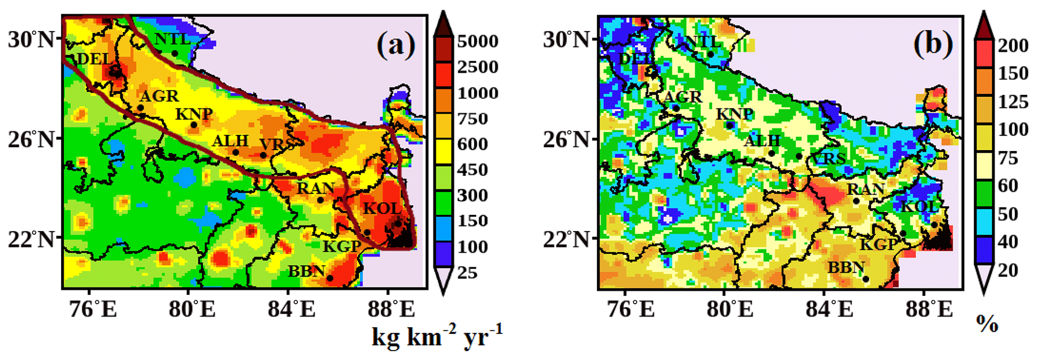
Figure 1 Spatial distribution of (a) the mean and (b) percentage deviation (δ) of the BC emission flux from five BC emission inventories implemented in CHIMERE over the study domain; the brown line in (a) indicates the IGP region.

2.2 Observational data for model evaluation and model sensitivity analysis

The spatial distribution of WRF-simulated surface temperature over the IGP is compared with the available gridded distribution of observed temperature from the Climatic Research Unit (CRU) (Morice et al., 2012). The observed temperature from the CRU at a horizontal resolution of 0.5^∘ × 0.5^∘ is re-gridded to the same resolution (0.1^∘ × 0.1^∘) as that from WRF, and the bias in simulated temperature for each grid cell is calculated using Eq. (1). The temporal trend of WRF-simulated hourly mean of meteorological parameters (temperature, relative humidity) is also evaluated with that observed from available measurements at stations over the IGP (Table 2). The monthly mean simulated PBLH average is compared with that measured for available stations in Delhi (mean of hourly PBLH during 10:00–16:00 LT), Kharagpur (10:00–11:00 and 14:00–15:00 LT), Ranchi (at 14:30 LT), and Nainital (05:00–10:00 LT), corresponding to the overlapping time hours from measurements (Fig. 2l in Sect. 3.1). The vertical distribution of the wintertime monthly mean potential temperature (Stull, 1988) as obtained from WRF-simulated temperature is also compared with the measured vertical distribution of potential temperature for December (obtained for 2 d) at a station in Kanpur from an available study (Table 2), corresponding to the overlapping time hours (10:00–12:00 LT) from measurements.

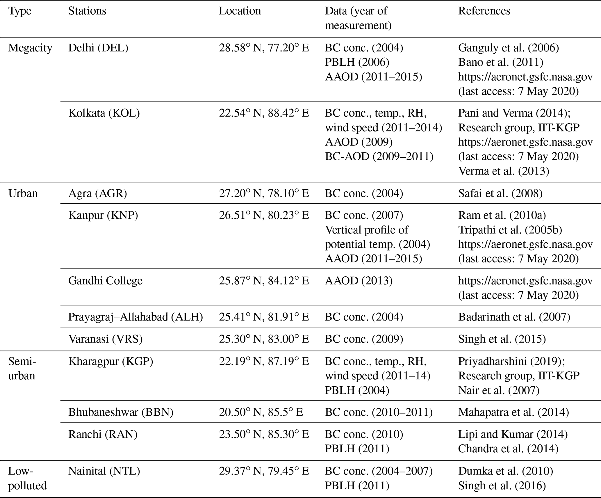
To compare the simulated BC surface concentration with observations, the measured BC surface concentration is obtained at stations over the IGP from available studies (refer to Table 2 and references therein). The selected stations correspond to area types identified as megacity (Delhi and Kolkata), urban (Agra, Kanpur, Prayagraj – or Allahabad, and Varanasi), semi-urban (Kharagpur, Ranchi, and Bhubaneshwar), and low-polluted (Nainital). Comparing model results with measurements thus aids in fulfilling the requirement to evaluate the model performance towards reproducing the observed spatial patterns in BC distribution for the various area types. Measurement data used in the present study are reported with an uncertainty (due to instrument artefacts, etc.) of about 10 %–30 % for PBLH (Seidel et al., 2010; Srivastava et al., 2010), 2 %–3 % for meteorological parameters, and 5 %–20 % for the measured BC concentration (refer to Table 2 for details and references therein). It is to be noted that observational data used for comparing model estimates (meteorological parameters and BC aerosols) are from measurements during different years at stations over the IGP. The inter-annual variability of the PBLH (based on observations over Delhi) is reported as within 10 % (Iyer and Raj, 2013), and for surface temperature (based on available measurement data from the India Meteorological Department over Kolkata and Kharagpur) it is less than 6 %. The inter-annual variability of the atmospheric BC concentration over the Indian subcontinent is obtained as 5 %–10 % (Safai et al., 2014; Surendran et al., 2013; Bisht et al., 2015; Ram et al., 2010b; Kanawade et al., 2014; Pani and Verma, 2014). This is taking into account that the reported inter-annual variability of meteorological parameters and the atmospheric BC concentration is nearly equivalent to or within the uncertainty range for measurements and is also much lower than the discrepancy between simulated and observed BC as reported in previous studies (refer to Sect. 1). The uncertainty range is taken into consideration while evaluating the model performance compared to measurements. The comparison between model estimates and measurements at widespread geographical locations and area types as presented in this study is therefore justified and is primarily required for evaluating the model performance and enhancing the statistical analysis.

The model-estimated and measured BC concentrations are compared corresponding to daytime (10:00–16:00 LT) and all-day (24-hourly) winter monthly mean values. This comparison is made because measured BC concentrations are found to exhibit a strong diurnal variability, with a relatively lower value during daytime hours than during the late evening to early morning hours; this is attributed to prevailing wintertime meteorological conditions (Verma et al., 2013; Pani and Verma, 2014). Also, the daytime mean BC concentration exhibits low hourly variability and corresponds to the well-mixed layer of the atmosphere (Verma et al., 2013; Pani and Verma, 2014). Hence, the lower value of the daytime mean from the model than from observations is primarily attributable to a low emission strength. Evaluation of model estimates for both the daytime and all-day mean thus provides a systematic hypothetical approach to identify the model discrepancy if primarily due to emissions or due to model processes attributed to meteorology (which is an input to the various aerosol processes that govern the atmospheric residence time of aerosols). This approach is further strengthened by implementing BC emissions from five new BC emission inventory databases and simulating BC transport subjected to the same aerosol physical and chemical processes with CHIMERE.

Bias in simulated estimates (X^modelled) from simulations at stations mentioned above for hourly, all-day, and daytime hours is estimated with respect to observed data (X^obs) with the equation as follows:

$$\begin{array}{}\text{(1)}& \mathrm{Bias}={\displaystyle \frac{(X^{\mathrm{modelled}}-X^{\mathrm{obs}})}{X^{\mathrm{obs}}}}\times \mathrm{100}\mathit{\%},\end{array}$$

where X=BC concentration, temperature, relative humidity, wind speed, and PBLH.

Statistical analyses are carried out corresponding to daytime and all-day winter monthly mean to evaluate the normalised mean bias (NMB, Eq. 2) and root mean square error (RMSE, Eq. 3) from the simulated results for N (N=10 in this study) stations. We also evaluate the percentage deviation (δ) in the simulated BC concentration attributed to BC emissions, estimated as the variability about the mean of the BC concentration from five simulations (refer to Eq. 4).

Further, the BC-AOD estimated in the present study (refer to Sect. 2.3) is compared with aerosol absorption optical depth (AAOD) from Aerosol Robotic Network (AERONET; level: 2) measurements over the IGP (Giles et al., 2012; Holben et al., 1998) at stations in Kanpur, at New Delhi IMD, at Gandhi College (25.87^∘ N, 84.12^∘ E), and at the IIT Kharagpur extension in Kolkata. The wintertime AAODs available from AERONET observations for Kanpur, New Delhi IMD, Gandhi College (December 2010–2015 averaged), and Kolkata (February 2009 averaged) are used in the comparison. For Kolkata, the comparison is also made with the estimated BC-AOD for the December 2010 period as obtained from the configured aerosol model using in situ ground-based observations for the same period (Verma et al., 2013). The AERONET AAOD data are available at four wavelengths: 440, 675, 870, and 1020 nm. The AAOD at the wavelength of 550 nm (used for comparison with simulated BC-AOD in the present study) is obtained based on the wavelength dependence of AAOD as per Giles et al. (2012).

A correlation study is also carried out between the variance of emissions and simulated BC concentrations or simulated BC-AOD from the simulations to examine the sensitivity of the simulated BC concentration or BC-AOD to the variation in emission magnitude.

$$\begin{array}{}\text{(2)}& {\displaystyle }\mathrm{NMB}={\displaystyle \frac{\sum _{\mathrm{1}}^N\left|{\mathrm{BC}}^{\mathrm{modelled}}-{\mathrm{BC}}^{\mathrm{obs}}\right|}{\sum _{\mathrm{1}}^N{\mathrm{BC}}^{\mathrm{obs}}}}\times \mathrm{100}\mathit{\%}\text{(3)}& {\displaystyle }\mathrm{RMSE}={\left[{\displaystyle \frac{\mathrm{1}}{N}}\sum _{\mathrm{1}}^N({\mathrm{BC}}^{\mathrm{modelled}}-{\mathrm{BC}}^{\mathrm{obs}}{)}^{\mathrm{2}}\right]}^{\frac{\mathrm{1}}{\mathrm{2}}}\text{(4)}& {\displaystyle }\mathit{\delta }={\displaystyle \frac{\mathit{\sigma }}{\mathrm{mean}}}\times \mathrm{100}\mathit{\%}\end{array}$$

Here, σ is the standard deviation for the mean from five simulations (e.g. BC emissions, all-day, daytime mean of BC concentration).

Ganguly et al. (2006)Bano et al. (2011)Pani and Verma (2014)Verma et al. (2013)Safai et al. (2008)Ram et al. (2010a)Tripathi et al. (2005b)Badarinath et al. (2007)Singh et al. (2015)Priyadharshini (2019)Nair et al. (2007)Mahapatra et al. (2014)Lipi and Kumar (2014)Chandra et al. (2014)Dumka et al. (2010)Singh et al. (2016)

Table 2 Observational data used for model validation from available studies at identified locations over the study domain.

2.3 Simulation of wintertime BC-AOD and radiative perturbations due to BC over the IGP

The BC-AOD is estimated with OPTical properties SIMulation (OPTSIM) (Stromatas et al., 2012) using the three-dimensional BC mass concentration obtained from CHIMERE corresponding to each of the five simulations (refer to Table 1). Aerosol optical properties are estimated based on Mie theory calculations considering internal mixing (Lesins et al., 2002; Permadi et al., 2018b). These estimations are done at six wavelengths of 440, 500, 532, 550, 870, and 1064 nm and the same horizontal and temporal resolution as of CHIMERE.

For radiative transfer calculations, estimates from the Constrained simulation (which is determined to be the most efficient to simulate the BC distribution, as discussed later) and the Smog simulation (from India-based BC emissions as a representative bottomup simulation) are only considered. For estimating the radiative effect due to BC aerosols, simulation of aerosol optical properties (AOD, single-scattering albedo – SSA, and the Ångström exponent – AE) is conducted with OPTSIM for three different cases considering (i) the atmosphere including BC (with BC, BCaero), (ii) the atmosphere without BC (without BC, wBC), and (iii) the atmosphere with no aerosol (without aerosol, wAero). The three-dimensional aerosol species concentration as an input to OPTSIM is derived for each of the three cases from CHIMERE corresponding to the simulations (Constrained and Smog simulations).

Aerosol radiative transfer calculations are done in WRF-Solar at a temporal resolution of 1 h and horizontal grid resolution of 0.1^∘ × 0.1^∘ by selecting a regular longitude–latitude projection. The WRF Preprocessing System (WPS) internally converts the grid resolution corresponding to longitude–latitude projection from degrees to metres as required for model processing. WRF-Solar is a new version of the WRF model enhanced for the prediction of solar irradiance (Haupt et al., 2016; Jimenez et al., 2016). The meteorological initial and boundary conditions provided to the model are as per the WRF model, as mentioned previously (refer to Sect. 2.1.2). The Rapid Radiative Transfer Model for GCMs scheme (RRTM-G) (Iacono et al., 2008) is selected for shortwave and longwave radiation. The direct and diffused components of solar irradiance are separately addressed with the RRTM-G scheme to improve the model calculations by considering surface irradiance components in the estimation.

Simulations for radiative flux with WRF-Solar are performed for each of the three cases, as mentioned above, using respective simulated optical properties as input for each case. The shortwave (SW) radiative flux (at 550 nm) for clear-sky conditions is estimated at the top (TOA) and bottom (SUR) layer of the atmosphere for the atmosphere with BC and without BC. This is done by subtracting the respective flux at TOA and SUR due to wAero from the flux due to wBC and BCaero, respectively. The direct radiative perturbations or the direct radiative effects (DREs) due to BC aerosols at TOA (DRE^TOA(BC)) and at SUR (DRE^SUR(BC)) are calculated by taking the difference between the radiative flux from BCaero and that from wBC at the respective layers of the atmosphere (Eqs. 5 and 6). The DRE in the atmosphere (ATM) due to BC is estimated by subtracting the flux at the SUR from that estimated at TOA (Eq. 7).

$$\begin{array}{}\text{(5)}& {\displaystyle }\begin{array}{rl}{\mathrm{DRE}}^{\mathrm{TOA}}\left(\mathrm{BC}\right)& =\left[{\mathrm{DRE}}^{\mathrm{TOA}}\right(\mathrm{BCaero})-{\mathrm{DRE}}^{\mathrm{TOA}}(\mathrm{wAero}\left)\right]\\ & -\left[{\mathrm{DRE}}^{\mathrm{TOA}}\right(\mathrm{wBC})-{\mathrm{DRE}}^{\mathrm{TOA}}(\mathrm{wAero}\left)\right]\end{array}\text{(6)}& {\displaystyle }\begin{array}{rl}{\mathrm{DRE}}^{\mathrm{SUR}}\left(\mathrm{BC}\right)& =\left[{\mathrm{DRE}}^{\mathrm{SUR}}\right(\mathrm{BCaero})-{\mathrm{DRE}}^{\mathrm{SUR}}(\mathrm{wAero}\left)\right]\\ & -\left[{\mathrm{DRE}}^{\mathrm{SUR}}\right(\mathrm{wBC})-{\mathrm{DRE}}^{\mathrm{SUR}}(\mathrm{wAero}\left)\right]\end{array}\text{(7)}& {\displaystyle }{\mathrm{DRE}}^{\mathrm{ATM}}\left(\mathrm{BC}\right)={\mathrm{DRE}}^{\mathrm{TOA}}\left(\mathrm{BC}\right)-{\mathrm{DRE}}^{\mathrm{SUR}}\left(\mathrm{BC}\right)\end{array}$$

3 Results and discussion

3.1 Analysis of WRF-simulated meteorological parameters

The WRF-simulated winter monthly mean distribution of the horizontal wind speed, vertical wind velocity, and PBLH over the IGP are presented in Fig. 2a–c. As observed from the wind field distribution map, there is a predominance of weak north-easterlies (1–2 m s⁻¹) over the IGP. The vertical wind velocity distribution indicates a neutral air mass or a downdraft of the air mass over the IGP (a positive value of the vertical wind velocity is an indication of a downdraft of the air mass and vice versa). The presence of a narrow PBLH (200 to 600 m) over most of the IGP indicates low vertical mixing during winter (Fig. 2c). The topographical elevation decreases from the northern IGP towards the eastern IGP, with the maximum elevation observed on the northward side due to the Himalayan mountains (Fig. 2d).

Figure 2 Spatial distribution of the WRF-simulated (a–c) winter monthly mean (a) horizontal wind field (note that the colour scale is for wind speed in m s⁻¹ and the arrows indicate the direction of the mean field), (b) vertical wind speed at 1000 hPa, (c) planetary boundary layer height (PBLH in metres), and (d) topography (metres above sea level, m a.s.l.) (e–g) Spatial distribution of winter monthly mean surface temperature from (e) WRF simulations, (f) observations from CRU, and (g) percentage bias in WRF estimates. (h–k) Comparison of the hourly distribution of winter monthly mean (h, j) surface temperature and (i, k) relative humidity from WRF simulations with observations at stations (Kharagpur, KGP; Kolkata, KOL). (l) Comparison of winter monthly mean PBLH during day hours between measured and simulated values at the stations under study. The error bars represent the standard deviation (σ) in the measured PBLH. (m) Comparison of the vertical profile of potential temperature obtained from WRF (winter monthly mean) and measurements (2 d).

A high load of BC aerosols over the IGP as obtained (discussed later) in the present study is inferred due to confinement of pollution near the surface within the shallow boundary layer height in winter due to low vertical mixing and weak dispersion of atmospheric pollutants. This creates stagnant weather under the prevailing meteorological conditions, with low temperature, weak wind speed, the downdraft of the air mass, and a narrow PBLH (as presented above). In addition, the Himalayan mountains northward further inhibit the dispersion of aerosol pollutants and favour their confinement over the IGP. This inference is also in corroboration with observational studies at stations over the IGP (e.g. Nair et al., 2007, 2012; Pani and Verma, 2014; Verma et al., 2014; Vaishya et al., 2017; Rana et al., 2019). Further, the IGP also comprises the highest population density and therefore enhanced BC emission strength during winter, specifically from biofuel combustion, e.g. fuelwood and crop waste for residential cooking and heating (Venkataraman et al., 2005; Sahu et al., 2015; Verma et al., 2017; Rana et al., 2019).

We compare the spatial distribution of monthly mean temperature from WRF simulations (Fig. 2e) with that from gridded ground-based observations from CRU (Fig. 2f). The bias in model-estimated temperature is found to be within ± 5 % over most of the IGP (Fig. 2g) but is noticed to be slightly large (about ± 10 % to ± 25 %) over a few grids in the north-eastern, western, and southern IGP. A comparative study of the hourly distribution of the winter monthly mean simulated surface temperature and relative humidity (RH), with the corresponding observed value from available measurements at Kharagpur (semi-urban) and Kolkata (megacity), is presented in Fig. 2h–k. Please refer to Table 2 for details on observational data. The temporal trend of the simulated hourly winter monthly mean of meteorological parameters conforms to the measurements. The magnitude of the hourly distribution of the winter monthly mean surface temperature from simulations (Fig. 2h and j) is found to compare well with that from observations during daytime hours (10:00–16:00 LT) for both stations; it is, however, seen to be underestimated (bias: −45 % to −58 %) during midnight to early morning hours (00:00–05:00 LT). The WRF-simulated meteorology is input to various aerosol processes that govern the atmospheric residence time of aerosols in CHIMERE and thereby influences the atmospheric concentration of BC aerosols. A lower value of simulated surface temperature than observed during midnight to early morning hours would lead to decreased mixing of pollutants, enhancing their accumulation in the atmosphere during these hours (as also evinced in the diurnal distribution of the simulated BC concentration; refer to Sect. 3.2, Fig. 4).

The WRF-simulated RH at both stations (Fig. 2i and k) is in good agreement with measurements (bias: −5 % to +35 %), with the mean RH during late evening to early morning hours (20:00–05:00 LT) being 2 times higher than that during daytime. A comparison of winter monthly mean PBLH during daytime hours (as described in Sect. 2.2) from the WRF simulation with that available from observations at Delhi, Kharagpur, Ranchi, and Nainital is also presented (Fig. 2l). The standard deviations (1σ) in measured PBLH values are within 10 %–16 % for Delhi, Kharagpur, and Ranchi and about 49 % at Nainital. The simulated PBLH is close enough to measurements (bias estimated within ±10 %) at all stations. Although at Nainital the simulated bias is large (−28 %), it is within the range of uncertainty in observations as mentioned in Sect. 2.2. The vertical profile of potential temperature (Fig. 2m) from WRF (wintertime monthly mean) resembles that measured at a station in Kanpur, with the bias being less than 4 % up to the height of 500 m and less than 1 % at a higher altitude (> 500 m).

Thus, the WRF-simulated winter monthly mean of the meteorological parameters, including their temporal trend, conforms well with the observations. However, it is required to reduce the discrepancy, specifically in the simulated magnitude of temperature during midnight to early morning hours. A better temporally resolved meteorological boundary condition in WRF (compared to 6-hourly from NCEP in the present study), aided by data assimilation at a fine temporal resolution (e.g. 1-hourly) using diurnal meteorological observations for India-based stations, would potentially lead to more accurate simulation of the observed magnitude of the diurnal distribution of meteorological parameters; an assessment in this regard is required in a future study.

3.2 Simulated wintertime BC concentration with new BC emissions as modelled with CHIMERE: impact of changing emissions and comparison with measurements

The spatial distribution of the winter monthly mean BC surface concentration from five simulations over the IGP is shown in Fig. 3a–e. The simulated mean BC concentration from the Constrained simulation is, in general, 2 to 4 times higher than that derived from the bottomup simulation over most of the IGP. Five hotspots or patches (refer to Fig. 3e) with a large BC concentration (magnitude > 16 µg m⁻³) from the Constrained simulation are identified in and around megacities (Delhi and Kolkata), in surrounding semi-urban areas, in urban spots over the central (Prayagraj–Allahabad–Varanasi) and mideastern IGP (Patna), and in one rural spot over the lower mideastern IGP (Palamu). It is interesting to see that the hotspots observed in the Constrained simulation are also identified in the Pku simulation, mostly in the Smog simulation as well, though with a smaller value than the Constrained simulation. Estimates from the Edgar and Cmip simulations simulate the megacity hotspots but fail to show the other identified hotspots in the Constrained simulation. Interestingly, the hotspot at Palamu (a coal-mining belt in Jharkhand) is simulated in the Constrained and Pku simulations, unlike the rest of other simulations, thereby suggesting a lack of BC emission source strength corresponding to Palamu and other identified hotspot locations in bottom-up BC emissions (as also mentioned in Sect. 2.1.3). The simulated spatial pattern (refer to Fig. 3f–g) of the BC surface concentration in the Constrained simulation, while exhibiting the lowest value at high-altitude and low-polluted locations (e.g. Nainital), moderately high values at semi-urban stations (e.g. Kharagpur and Ranchi), and high values at urban stations (e.g. Agra, Kanpur, Allahabad–Prayagraj, Varanasi), is seen to reach a maximum in megacities (Kolkata and Delhi). In comparison to the Constrained simulation, the simulated spatial gradient within and across the area types is seen to be inconsistent in bottomup simulation estimates. For example, the bottomup estimated values of the BC concentration from the Smog and Cmip simulations have a low spatial gradient from the megacity (Kolkata) to urban area type, including a lack of spatial contrast compared to the observations among the urban stations; the Pku simulation overestimates the all-day mean BC concentration for megacities but simulates the spatial gradient relatively well across the area types. The Edgar simulation matches the observed values well in megacities for the all-day mean but then underestimates the observations by a large value and with a low spatial contrast among the urban and semi-urban stations.

The simulated spatial pattern in the Constrained simulation is consistent with observations (Fig. 3f–g), as the BC distribution features for the specific area types are represented well by the simulated BC distribution. The spatial feature also indicates that the wintertime all-day mean value of the BC concentration (Fig. 3g) in Delhi is lower than Kolkata and vice versa for the daytime mean value (Fig. 3f), although the BC emission strength (refer to Fig. 1a) of the two megacities, Delhi and Kolkata, is nearly equivalent. We discuss these features in context with the transport of BC aerosols over the IGP based on the visualisation of an animation (https://doi.org/10.5446/48819; Ghosh and Verma, 2020) later in the section. The simulated magnitude of the BC surface concentration from the Constrained simulation, compared to that from the bottomup simulations, resembles the measured counterpart relatively well (Fig. 3f–g), with the ratio of the measured to simulated all-day (daytime) mean BC concentration being equivalent to nearly 1. A detailed statistical analysis of the comparison between simulated and observed BC is presented later in this section.

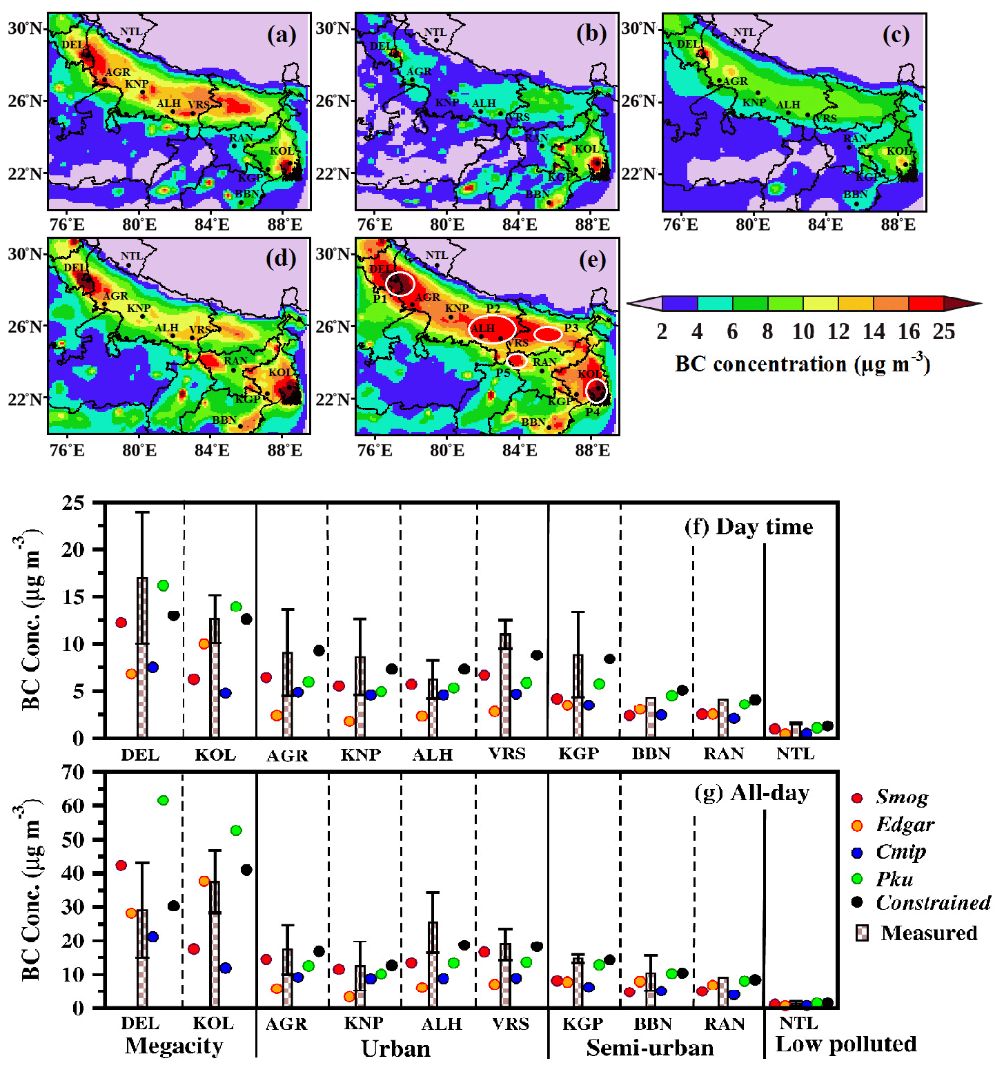
Figure 3 (a–e) Spatial distribution of simulated winter monthly mean BC surface concentration from the simulations (a) Smog, (b) Edgar, (c) Cmip, (d) Pku, and (e) Constrained; the circles in white in (e) represent the hotspots with patches of high BC concentrations. P1: Delhi patch, P2: Prayagraj–Allahabad–Varanasi patch, P3: Patna patch, P4: Kolkata patch, P5: Palamu patch. (f–g) Comparison of simulated monthly (f) daytime and (g) all-day mean BC surface concentration from five simulations with measurements at respective stations under study over the IGP; error bars represent the standard deviation (1σ) in the measured BC concentration.

The mean and standard deviation of the simulated BC concentration from five simulations at stations under study are provided in Table 3a (also refer to Fig. 4). Analysis of multi-simulations indicates that the percentage deviation (δ, refer to Eq. 4) in the simulated BC concentration (Table 3a) attributed to emissions is specifically the lowest for the low-polluted location (e.g. Nainital) and is generally within 40 % for all other locations under study. The δ for the megacity is noted as being typically more amplified (51 %–56 %) during the late evening to early morning hours (Table 3a, Fig. 4) than during daytime hours (35 %–43 %) compared to other locations under study. This suggests that under similar meteorological conditions and with the same aerosol processes in the model, the deviation in the simulated BC concentration can be attributed to emissions increases from daytime to late evening hours, thus indicating that increased emissions potentially amplify the accumulation of BC pollutants and worsen air quality over megacities, specifically during the late evening to morning hours compared to daytime hours, raising concern for megacity commuters.

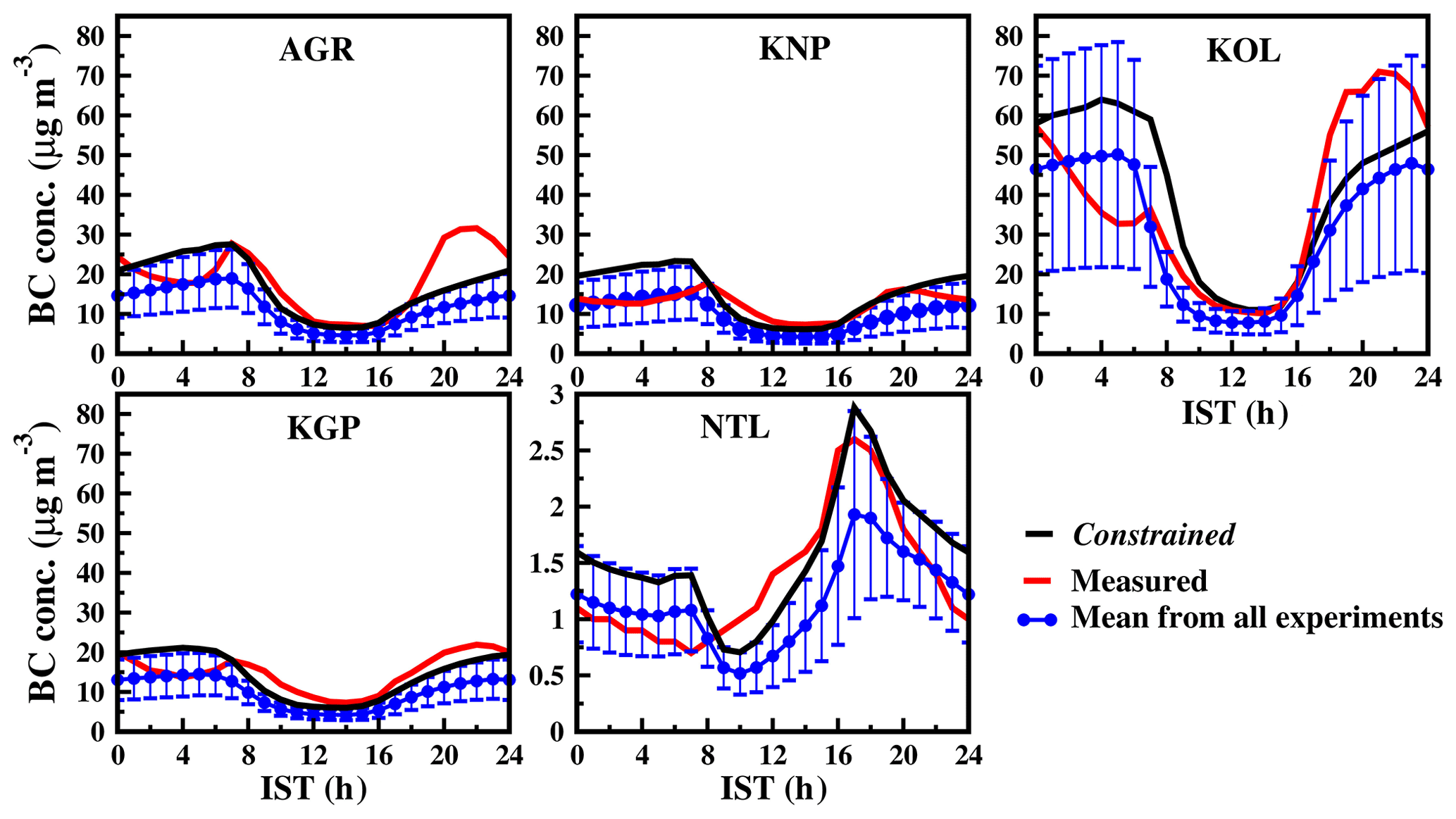
Figure 4 Hourly distribution of winter monthly mean BC concentration (µg m⁻³) at stations from the Constrained simulation (black line). Note that the y axis is on a different scale for Nainital. The mean and the standard deviations (1σ) from the five simulations corresponding to the hourly winter monthly mean BC concentration are also shown.

On comparing the temporal distribution of the simulated BC concentration from the Constrained simulation with that of the measured concentration, it is seen that the pattern of simulated diurnal variability (shown for selected stations; refer to Fig. 4) is consistent with that measured. The diurnal variability of the BC concentration is relatively higher, by a factor of 2 to 5, in the Constrained simulation during the late evening to early morning hours (20:00–05:00 LT) than during daytime hours (10:00–16:00 LT) at all stations (except Nainital). Notably, this factor is equivalent to that obtained from the bottomup simulations and also to that from observations (Surendran et al., 2013; Pani and Verma, 2014; Ram and Sarin, 2010; Nair et al., 2012; Dumka et al., 2010; Lipi and Kumar, 2014). The diurnal variability in the BC surface concentration is mainly associated with the atmospheric mixing depth depending upon the stability characteristics of the atmospheric layer linked with meteorology (Stull, 2012; Verma et al., 2013; Govardhan et al., 2015, 2019). It is worth noting that a specific feature is observed in the temporal trend of the BC concentration, which is the peak BC concentration during late afternoon hours (15:00–18:00 LT) at the high-altitude location of Nainital, unlike the temporal trend at plains locations (e.g. Kolkata, Kharagpur). This specific feature conforms with measurements and, as inferred from available studies (Dumka et al., 2010; Stull, 2012), is attributed to the deepening of the atmospheric mixing depth during the late afternoon hours, which flushes out pollutants, including BC, to high-altitude locations from the valley (Dumka et al., 2010; Stull, 2012). The distinct diurnal trend seen in the BC surface concentration at Nainital, in conjunction with the visualisation of the animation (https://doi.org/10.5446/48819; Ghosh and Verma, 2020; also discussed later in the section), thereby suggests the transport of BC pollution from the IGP towards the high-altitude Himalayan station of Nainital. However, the BC emission strength at Nainital is relatively lower than the IGP (refer to Fig. 1a). Therefore, consistent with observational studies, the simulated atmospheric BC concentration is noted to be the lowest at Nainital among the stations under study.

The bias in the simulated hourly distribution of the winter monthly mean BC concentration (refer to Fig. 4) with respect to observations is, however, noted to be larger by 40 %–60 % during midnight to early morning hours (00:00–05:00 LT) than during daytime hours. A larger bias is attributable to the simulated aerosol processes in CHIMERE being influenced by the simulated diurnal meteorology from the WRF. It is to be noted that the WRF-simulated hourly mean temperature is found to be 45 %–60 % lower than observed, specifically during 00:00–05:00 LT (as mentioned in Sect. 3.1), which has implications for the diurnal distribution of the BC concentration. In addition, an enhanced accumulation of BC concentration during late evening hours (18:00–22:00 LT), specifically for megacity (e.g. Kolkata) and urban locations (e.g. Agra), is noticed in the measurements compared to simulated values, thereby indicating the requirement to improve the representation of the factors for the hourly disaggregation of the total emission of pollutants in CHIMERE (Menut et al., 2012) during late evening hours (18:00–22:00 LT), specifically for megacity (e.g. Kolkata) and urban location (e.g. Agra). This improvement is suggested to take into account enhanced traffic emissions from heavy-duty commercial vehicles (Ganguly et al., 2006; Bano et al., 2011; Kumar et al., 2020) at these locations during late evening hours, hence requiring a better representation of the factors accounting for this enhancement. The results of the diurnal BC distribution, including improved representation of local emissions (specifically for megacity and urban locations) in CHIMERE forced by assimilated diurnal meteorological data, will be presented in a future study.

We also provide an animation showing a representation of the transboundary movement of BC pollutants over the IGP in the “Video supplement” (https://doi.org/10.5446/48819; Ghosh and Verma, 2020). This animation shows the hourly monthly mean surface BC concentration to highlight the diurnal cycle, and its visualisation shows the diurnal evolution of the plume of the BC surface concentration over the IGP. The BC surface plume is observed to be shrinking in magnitude during daytime hours (10:00–16:00 LT) and swelling up during evening until morning hours (18:00–06:00 LT). It is visualised spreading towards the north (Himalayan side, Nainital) during afternoon hours (12:00–18:00 LT), towards the south (central India), and from the upper northern IGP (e.g. Delhi) towards the lower eastern IGP (e.g. Kolkata). The diurnal feature of the surface BC plume distribution thereby appears to exhibit the pollution pattern of the IGP region.

The megacity of Delhi is surrounded by landmass on all sides and, as visualised from the animation, is influenced by the transport of pollutants from nearby regions (e.g. Punjab–Haryana) towards Delhi. In contrast, the megacity of Kolkata is a coastal location, and the atmospheric BC concentrations are also affected by the prevailing land–sea breeze activity there (Verma et al., 2016). A relatively lower daytime mean BC concentration measured at Kolkata than Delhi (Fig. 3f) is due to dilution of the aerosol pollutant concentration with the relatively pristine maritime air mass (attributed to the prevailing low-intensity sea breeze during winter). In contrast to the daytime mean, the higher all-day mean BC surface concentration at Kolkata compared to Delhi (Fig. 3g) is due to the outflow of BC pollutants from the upper northern IGP towards eastern IGP at Kolkata (https://doi.org/10.5446/48819; Ghosh and Verma, 2020). The outflow is visualised to be comparatively stronger during the evening until early morning hours (18:00–06:00 LT). In addition, the enhanced amplitude of the BC concentration at Kolkata compared to Delhi during the late evening is also due to the increased accumulation of BC pollutants owing to the land-breeze activity during winter (Verma et al., 2016).

The correlation coefficient (r) between the estimated and measured BC concentration for stations under study corresponding to each of the five simulations is also presented in Table 3b. A strong correlation is seen between model estimates and observations for both the all-day and daytime mean BC concentration from each of the five experiments. The above analyses indicate that the temporal pattern, including the spatial trend (as discussed before) of the BC distribution attributed to model processes (which govern the atmospheric residence time of BC; refer to Sect. 1), is simulated consistently well over the IGP, irrespective of the magnitude of the BC emission strength used in simulations.

Table 3 (a) Estimated mean and percentage deviation (δ, refer to Eq. 4) of the BC concentration from five simulations for the locations under study. (b) Summary of statistical analysis comparing the simulated BC concentration with measurements.

^* Number of stations from the stations under study with the percentage bias in simulated estimates calculated as ≤ ± 25 % (best efficiency), > ± 25 % to ± 50 % (moderate efficiency), and > ± 50 % (low efficiency).

Further, to statistically evaluate the simulated BC concentration from each of the five simulations with respect to observations, we define the performance of the simulation considering the best, moderate, and poor efficiency based on their relative frequency to maintain the percentage bias in the all-day (daytime) mean simulated BC concentration as about ≤ ± 25 %, > ± 25 % to ± 50 %, and > ± 50 %, respectively (refer to Table 3b), corresponding to the observation data points under study. This consideration leads us to identify the Constrained simulation estimates as delivering the best performance (percentage bias ≤ ± 25 %) among all simulations most of the time, i.e. for 100 % (100 %) of the total data points corresponding to the measured value at stations under study. Estimates from Pku exhibit the best performance for about 50 % (50 %) of the total stations. Those from the Smog and Edgar simulations are about 40 % (10 %) of the total stations under study. Estimates from the Smog and Edgar simulations are the most frequent, corresponding to moderate and poor efficiency, respectively. Notably, unlike the Constrained simulation, the best efficiency is infrequent (< 10 %), specifically for the daytime mean BC concentrations from the Smog, Edgar, and Cmip simulations, thereby indicating that the BC emission strengths of the respective emission database as input in the model are insufficiently low to simulate the BC distribution adequately over the IGP. A summary of statistical analysis with respect to the Pearson correlation (r), NMB, and RMSE accounting for estimates of the BC concentration from all simulations is also presented in Table 3b. The NMB (%) and RMSE (µg m⁻³) values for the all-day (daytime) mean BC concentration from the Constrained simulation are about 14 % (17 %) and 3 (2) µg m⁻³, which are the lowest among all of the simulations. The NMB from the Constrained simulation is noted as being within the uncertainty limits reported in BC measurements (5 %–20 %).

3.3 Simulated wintertime BC-AOD with new BC emissions: correlation analysis of variance

To evaluate the columnar distribution of wintertime BC aerosols over the IGP, the spatial distribution of the monthly mean BC-AOD at 550 nm from simulations is presented in Fig. 5a–e. The spatial pattern of the BC-AOD distribution, showing a large value over the IGP, is consistent with the features of observed AOD from satellite retrievals (e.g. Verma et al., 2014). The value of the BC-AOD distribution across the IGP from the Constrained simulation (0.04–0.1) is found to agree well with that from a recent study (0.05–0.1) based on a designed constrained aerosol simulation approach inferred as delivering good agreement between model estimates and observations of atmospheric aerosol species (Kumar et al., 2018; Santra et al., 2019). The BC-AOD from the Constrained simulation is also found to consistently match (NMB: 11 %) the absorption AOD (AAOD) from AERONET-based observations at stations over the IGP (Kanpur, New Delhi IMD, Gandhi College at 25.87^∘ N, 84.12^∘ E, IIT Kharagpur extension at Kolkata) and BC-AOD estimated at Kolkata from the configured aerosol model using in situ ground-based observations for Kolkata (Verma et al., 2013) (refer to Fig. 5f). Estimated BC-AOD from the simulations Pku, Smog, Cmip, and Edgar is lower in magnitude by 15 %–30 %, 30 %–50 %, 40 %–60 %, and 50 %–70 %, respectively, than the Constrained simulation over most of the IGP. An overall comparison of the Constrained and bottomup estimates with measurements thus indicates the low magnitude and inconsistent spatial gradient across area types of the bottom-up BC emission flux as the primary reason for a large discrepancy in the simulated BC concentration and BC-AOD from the bottomup simulation.

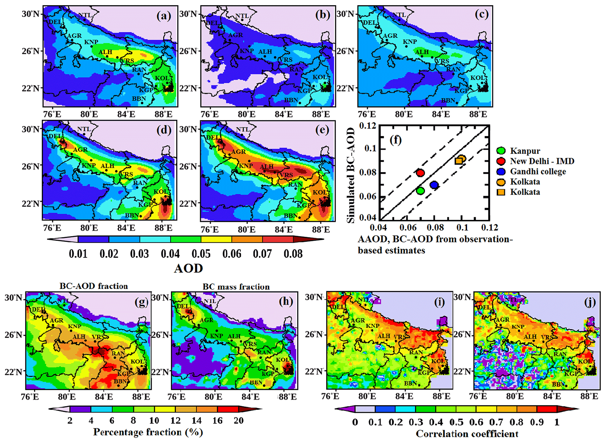
Figure 5 (a–e) Spatial distribution of simulated winter monthly mean BC-AOD at 550 nm over the IGP from the simulations (a) Smog, (b) Edgar, (c) Cmip, (d) Pku, and (e) Constrained. (f) Comparison of simulated BC-AOD from the Constrained simulation with the AAOD represented as circles (from AERONET-based observations at stations at Kanpur, New Delhi IMD, Gandhi College, and the IIT Kharagpur extension at Kolkata) and with BC-AOD represented as a square estimated using in situ ground-based observations at Kolkata; the dashed lines correspond to the value within ± 25 % of the 1 : 1 comparison shown as a solid line. (g–h) Spatial distribution of the (g) BC-AOD fraction (%) and (h) BC mass fraction (%) from the Constrained simulation. (i–j) Correlation between the variance in the BC emission flux from five BC emission databases and in estimated (i) BC-AOD and (j) BC concentration from five simulations.

The percentages of BC-AOD fraction and BC mass fraction from the Constrained simulation (Fig. 5g–h) are estimated by taking the ratio of BC-AOD to total AOD and that of the BC concentration to the total submicron aerosol concentration, respectively. The total AOD and submicron aerosol concentration required for estimating the fractional distribution are obtained from a previous study (as mentioned above) based on the designed constrained aerosol simulation approach (Kumar et al., 2018). The BC-AOD fraction and BC mass fraction are about 10 %–16 % and 6 %–10 %, respectively, over most of the IGP. The estimated BC mass fraction in the present study is also seen to be in corroboration with values reported from wintertime measurements over the Indian region, e.g. noted as being 12 % (wintertime average) of the total submicron aerosol concentration over Kolkata, 4 %–15 % of the total aerosol concentration over Delhi and Kanpur, and 3 %–7 % of PM_2.5 over Varanasi and Anantapur, including that over the Kaashidhoo climate observatory in the Maldives (Verma et al., 2013; Kumar et al., 2017; Tripathi et al., 2005a; Ganguly et al., 2006; Reddy et al., 2012; Satheesh et al., 1999). The location of hotspots for BC mass fraction (value > 16 %) and BC-AOD fraction (12 %–16 %), including that for BC-AOD (value > 0.08), is seen to overlap that identified for BC surface concentration (Fig. 3e). It is also seen that the percentage fraction of BC-AOD, in general, is about twice as large as the BC mass fraction, indicating that even a low BC concentration in aerosol mass has the potential to significantly contribute to attenuation of solar radiation and thereby influence the regional radiation balance (which is examined in the next section).

To gain insight into the degree of association of the simulated BC burden with the BC emission strength, we utilise the five simulations to evaluate the correlation coefficient between the variation in emission strength and that in simulated BC-AOD (Fig. 5i) or the simulated BC concentration (Fig. 5j). A strong correlation (correlation coefficient: > 0.7) is seen between the variance in BC emissions and simulated BC mass concentration or BC-AOD, e.g. as observed over most of the IGP region (including the megacity of Kolkata). The strong correlation is indicative of the change in the BC emission flux primarily governing the change in the simulated BC mass concentration and BC-AOD. On the other hand, a moderate correlation for the BC surface concentration (correlation coefficient: 0.5–0.6) is observed over parts of the lower mideastern IGP (patch P5; refer to Fig. 3e), over parts of the northern IGP (patch P1) including in and around the megacity of Delhi (for both BC surface concentration and BC-AOD), and over some parts of the eastern IGP (patch P4), including the area around the megacity of Kolkata. The moderate correlation suggests that over these parts, besides the change in BC emission strength, transport of BC aerosols as governed by model processes also has a profound impact on the simulated BC burden. In other words, a large BC burden over the megacity of Delhi and the surrounding region is profoundly impacted due to the transport of BC aerosols, in addition to the BC emission strength. A weak correlation (correlation coefficient: < 0.5), e.g. as observed over Nainital and Ranchi stations and the surrounding area, suggests that the transport of BC aerosols compared to the BC emission strength primarily influences the BC burden. It is also noted that over the central region (bounded between 76–80^∘ E and 20–26^∘ N), the correlation for BC-AOD is moderate but still stronger than the BC concentration, thereby indicating the potential influence on BC-AOD over the region from high-rising open burning BC emissions (corroborated by the prevalence of open biomass burning emissions; Venkataraman et al., 2006) and the elevated transport of BC aerosols as also inferred in a previous study (Verma et al., 2008).

3.4 Wintertime direct radiative perturbations due to BC aerosols: comparison with atmosphere-eliminating BC

Further, the wintertime SW direct radiative perturbation due to BC aerosols over the IGP (Fig. 6a–c) is evaluated corresponding to the layers of the atmosphere (SUR, ATM, and TOA; refer to Sect. 2.3). We also compare the direct radiative perturbation due to BC with that estimated considering atmosphere-eliminating BC or without BC aerosols (Fig. 6d–f) to evaluate the magnitude of direct radiative perturbation in the presence of BC aerosols. The positive value of the radiative effect signifies warming due to BC aerosols and vice versa for the negative value of the radiative effect. There is a reduction in the wintertime radiative flux due to BC at the SUR by −20 to −40 W m⁻² (Fig. 6a). The radiative warming (Fig. 6c) due to BC aerosols at the ATM (+30 to +50 W m⁻²) is estimated to be about 50 %–70 % larger than the cooling due to BC at the SUR. The magnitude of the SUR cooling effect as noted due to BC aerosols is, however, found to be 10 %–20 % lower than that estimated considering atmosphere-eliminating BC aerosols (Fig. 6d and g). Moreover, the magnitude of ATM radiative warming due to BC is seen to be larger by 2–3 times compared to the atmosphere without BC aerosols (Fig. 6f and h). The radiative effect at the TOA due to BC aerosols (Fig. 6b) is positive and thereby indicates a net radiative warming effect (+10 to +17 W m⁻²) over the IGP during winter. In contrast, a cooling effect at TOA (−10 to −20 W m⁻²) is exhibited considering the atmosphere without BC aerosols (Fig. 6e). It is also seen that the patch with the most substantial value (>15 W m⁻²) of net radiative forcing due to BC is observed in and around megacities and is extended to the eastern coast. A comparison of the radiative effect due to BC from Constrained estimates with that from the Smog simulation estimates shows that bottom-up BC emissions (e.g. Smog-India) lead to relatively lower wintertime radiative warming at ATM and TOA by 30 %–50 % than the Constrained_emiss emissions over most of the IGP and by more than 80 % over the northern IGP (in and around Delhi). The comparison between the bottomup and Constrained estimates thus indicates the potential underestimation of wintertime direct radiative perturbation due to BC aerosols over the IGP attributable to the low BC emission strength in the bottom-up BC emission database.

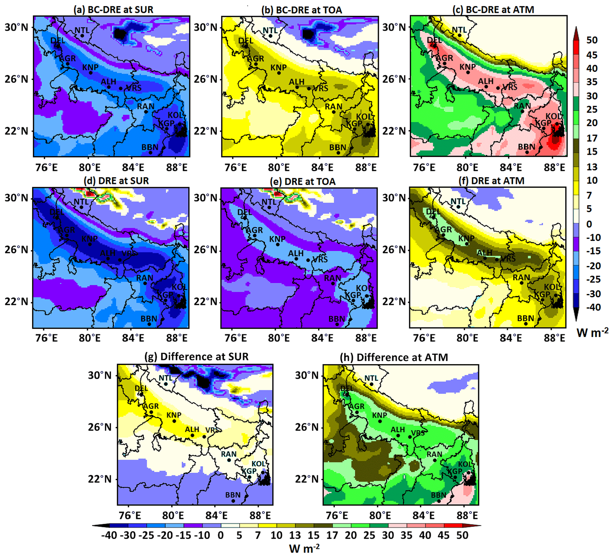
Figure 6 (a–c) Spatial distribution of wintertime direct radiative perturbation due to BC aerosols from the Constrained simulation at (a) SUR, (b) TOA, and (c) ATM. (d–f) Same as (a–c) but with atmosphere-eliminating BC. (g–h) Difference in radiative perturbation due to BC and atmosphere-eliminating BC at (g) SUR and (h) ATM.

The uncertainty in estimated wintertime direct radiative perturbations in the present study is inferred to be within 40 %. This estimation is based on taking into account NMB in the simulated BC concentration (as presented in Sect. 3.2) and the model variability (33 %) in estimated DRF of BC based on the evaluation of 20 global aerosol models (Schulz et al., 2006).

4 Conclusion

In the present study, wintertime direct radiative perturbation due to black carbon (BC) aerosols was examined over the Indo-Gangetic Plain (IGP) by evaluating the efficacy of the fine grid-resolved (0.1^∘ × 0.1^∘) BC aerosol transport in a chemical transport model (CHIMERE) offline coupled with the WRF regional meteorological model. The efficacy of CHIMERE to simulate the observed BC surface concentration was assessed by implementing the new BC emission inventories and through a detailed validation and statistical analysis of the simulated BC concentration with respect to ground-based measurements at stations over the IGP. The five BC transport simulations (Constrained and bottomup, with the latter including Smog, Cmip, Edgar, and Pku) were performed by implementing BC emission data from the India-based “Constrained_emiss” and bottom-up Smog-India database as well as those from the three global bottom-up databases CMIP6, EDGAR, and PKU extracted over the Indian region.

The WRF-simulated winter monthly mean of the meteorological parameters resembled (bias < ± 25 %) the measured counterparts. However, the diurnal distribution of meteorological parameters exhibited a considerable discrepancy, specifically during midnight to early morning hours (00:00 to 05:00 LT), having implications for the diurnal distribution of the BC concentration. In this regard, a better temporally resolved meteorological boundary condition in the WRF, aided by data assimilation at a fine temporal resolution (e.g. 1-hourly) using observations for India-based stations, needs to be assessed in a future study.

A strong association of the winter monthly mean BC concentration between modelled and measured values for stations under study corresponding to each of the five simulations was noticed. The efficacy to simulate the magnitude of the observed wintertime BC distribution was found to be moderate to poor for the bottomup simulation. The Constrained simulation estimated high BC pollution over the IGP, with a wintertime all-day monthly mean BC surface concentration (BC-AOD) of 14–25 µg m⁻³ (0.04–0.08), and resembled the observed counterparts. These estimates were noted with the lowest percentage bias (≤ ± 25 %) among five simulations for each of the stations and area types under study. The low magnitude and inconsistent spatial gradient across area types of the bottom-up BC emission flux were found to be the primary reasons for a large discrepancy in simulated BC concentration and BC-AOD from the bottomup simulation.

The BC-AOD fraction (10 %–16 %) from the Constrained simulation was noted to be about twice as large as the BC mass fraction (6 %–10 %) over most of the IGP region. Five hotspots with a large BC load (surface concentration > 16 µg m⁻³ from the Constrained simulation) were identified in and around megacities (Delhi and Kolkata) and the surrounding semi-urban area as well as urban spots over the central and mideastern IGP (Prayagraj–Allahabad–Varanasi, Patna), including the rural spot over the lower mideastern IGP (Palamu).

Analysis of multi-simulations of BC transport in CHIMERE indicated that increased emissions in the megacities potentially amplify the accumulation of BC pollutants, specifically during the late evening to morning hours, raising concern for megacity commuters. The correlation between the variance in emissions and the simulated BC mass concentration and BC-AOD from the five simulations manifested in the sensitivity of the simulated BC concentration and BC-AOD primarily to the change in BC emission strength over most of the IGP (including the megacity of Kolkata). There is also sensitivity to the transport of BC aerosols as governed by model processes over the megacity of Delhi and the area around the megacities of Delhi and Kolkata.

The transboundary movement of the wintertime BC plume in the IGP was visualised to be spreading towards the north (Himalayan side) during afternoon hours (12:00–18:00 LT) as well as towards the south (central India) and from the upper northern IGP (e.g. Delhi) towards the lower eastern IGP (e.g. Kolkata) during evening until morning hours (18:00–06:00 LT).

Analysis of direct radiative perturbations due to BC aerosols showed that wintertime BC aerosol over the IGP enhances atmospheric warming by 2–3 times more and reduces surface cooling by 10 %–20 % less than considering atmosphere-eliminating BC aerosols. The BC-induced net warming effect at the top of the atmosphere (TOA) from the Constrained simulation was estimated as 10–17 W m⁻² over most of the IGP, in contrast to a net cooling at the TOA considering the atmosphere without BC. The radiative perturbation was spatially the largest in and around megacities (Kolkata and Delhi) and extended to the eastern coast. Values were assessed to be about 30 %–50 % lower from the bottomup than the Constrained simulation over most of the IGP.

The present study showed that adequate BC emission strength and meteorological forcing in a state-of-the-art chemical transport model at a fine grid resolution led to the successful simulation of the wintertime BC distribution (surface concentration and BC-AOD) over the IGP, unlike previous studies (refer to Sect. 1). We believe this distribution provided a reasonably more accurate representation of the simulated wintertime direct radiative perturbations due to BC aerosols, including identifying the BC hotspots over the IGP. The wintertime radiative perturbation due to BC aerosols simulated in the present study is further utilised to evaluate the potential response to temperature, air quality, and regional climate over the IGP; the outcome from these evaluations will be presented in a future study. The present study is also further extended to evaluate the inter-seasonal BC distribution and associated radiative impacts over the Indian subcontinent, with implications for the south-west monsoon rainfall.