the Creative Commons Attribution 4.0 License.
the Creative Commons Attribution 4.0 License.
 | 05 May 2021
Analysis of recent lower-stratospheric ozone trends in chemistry climate models
Simone Dietmüller
Hella Garny
Roland Eichinger
William T. Ball
Recent observations show a significant decrease in lower-stratospheric (LS) ozone concentrations in tropical and mid-latitude regions since 1998. By analysing 31 chemistry climate model (CCM) simulations performed for the Chemistry Climate Model Initiative (CCMI; Morgenstern et al., 2017), we find a large spread in the 1998–2018 trend patterns between different CCMs and between different realizations performed with the same CCM. The latter in particular indicates that natural variability strongly influences LS ozone trends. However none of the model simulations reproduce the observed ozone trend structure of coherent negative trends in the LS. In contrast to the observations, most models show an LS trend pattern with negative trends in the tropics (20∘ S–20∘ N) and positive trends in the northern mid-latitudes (30–50∘ N) or vice versa. To investigate the influence of natural variability on recent LS ozone trends, we analyse the sensitivity of observational trends and the models' trend probability distributions for varying periods with start dates from 1995 to 2001 and end dates from 2013 to 2019. Generally, modelled and observed LS trends remain robust for these different periods; however observational data show a change towards weaker mid-latitude trends for certain periods, likely forced by natural variability. Moreover we show that in the tropics the observed trends agree well with the models' trend distribution, whereas in the mid-latitudes the observational trend is typically an extreme value of the models' distribution. We further investigate the LS ozone trends for extended periods reaching into the future and find that all models develop a positive ozone trend at mid-latitudes, and the trends converge to constant values by the period that spans 1998–2060. Inter-model correlations between ozone trends and transport-circulation trends confirm the dominant role of greenhouse gas (GHG)-driven tropical upwelling enhancement on the tropical LS ozone decrease. Mid-latitude ozone, on the other hand, appears to be influenced by multiple competing factors: an enhancement in the shallow branch decreases ozone, while an enhancement in the deep branch increases ozone, and, furthermore, mixing plays a role here too. Sensitivity simulations with fixed forcing of GHGs or ozone-depleting substances (ODSs) reveal that the GHG-driven increase in circulation strength does not lead to a net trend in LS mid-latitude column ozone. Rather, the positive ozone trends simulated consistently in the models in this region emerge from the decline in ODSs, i.e. the ozone recovery. Therefore, we hypothesize that next to the influence of natural variability, the disagreement of modelled and observed LS mid-latitude ozone trends could indicate a mismatch in the relative role of the response of ozone to ODS versus GHG forcing in the models.
- Article
(7331 KB) - Full-text XML
-
Supplement
(737 KB) - BibTeX
- EndNote


Stratospheric ozone is essential for protecting the Earth's surface from ultraviolet radiation, which is harmful for plants, animals, and humans. Human-made ozone-depleting-substance (ODS) emissions significantly reduced ozone concentrations for some decades after 1960. After controlling the use of ODSs by the 1987 Montreal Protocol and later adjustments, however, ODS concentrations started to decline in the mid to late 1990s (e.g. Newman et al., 2007; Chipperfield et al., 2017). As a consequence, total stratospheric ozone is expected to recover in the future. Dhomse et al. (2018) have analysed the recovery of stratospheric ozone mixing ratios of the CCMI-1 (Chemistry Climate Model Intercomparison project part 1) climate projection simulations. They found that the ozone layer is simulated to return to a pre-1980 ODS level between 2030 and 2060, depending on the region. However, they discovered a large spread among the individual models, which shows that there are many uncertainties in these projections. The evolution of stratospheric ozone in the 21st century results not only from a decrease in ODS concentrations but also from an interplay between changes in both the atmospheric composition and the circulation (World Meteorological Organization (WMO) 2014). Increasing anthropogenic greenhouse gas (GHG) emissions (CO2, CH4, N2O) leads to enhanced tropical upwelling and thereby to an acceleration of tracer transport along the stratospheric overturning circulation (e.g. Butchart, 2014; Eichinger et al., 2019). On the other hand, increasing GHG concentrations also slows down ozone depletion through GHG-induced stratospheric cooling (e.g. Jonsson et al., 2004; Oman et al., 2010; Bekki et al., 2013; Dietmüller et al., 2014; Marsh et al., 2016), and emissions of CH4 and N2O additionally impact ozone through chemical processes (e.g. Ravishankara et al., 2009; Kirner et al., 2015; Revell et al., 2012; Winterstein et al., 2019).
In recent years, a number of studies have analysed observational records to identify ozone trends in the stratosphere (e.g. Harris et al., 2015; Steinbrecht et al., 2017; Weber et al., 2018). These studies consistently report an ozone recovery in the upper stratosphere after the turnaround of the ODS concentrations around the year 1998. In the lower stratosphere (LS), however, most observed ozone trends are not statistically significant for such a relatively short period due to large internal variability and instrumental difficulties (e.g. Steinbrecht et al., 2017). Subsequently, Ball et al. (2018) analysed LS ozone trends from satellite data between 1998 and 2016 in detail, making use of a dynamical (multiple) linear regression analysis. They identified a statistically significant decline in LS ozone between 60∘ S and 60∘ N in that period of approximately 2 DU in the LS below 24 km altitude. The implication was that the stratospheric ozone column was continuing to decline because the LS ozone reduction more than offsets the positive trend in the upper stratosphere. Shortly afterwards Wargan et al. (2018) studied ozone trends in the reanalysis products MERRA-2 and GEOS-RPIT. In the tropics they detected a positive ozone trend in a 5 km layer above the tropopause and a negative trend at 7–15 km above the tropopause. Nevertheless, in the northern and southern mid-latitude LS they detected a negative ozone trend. As such, there are some similarities to the findings of Ball et al. (2018), but there are also quantitative differences, for example the positive trend in the 5 km layer or a missing overall statistically significant decrease in the column integrated ozone. Wargan et al. (2018) suggested that the negative mid-latitude trend might be explained by enhanced isentropic transport between the tropical and mid-latitude LS. However, the recent study of Orbe et al. (2020) explicitly demonstrated that in the Northern Hemisphere (NH) this mid-latitude ozone decrease is primarily associated with large-scale advection. Furthermore, they showed that the observed changes in advection and in ozone are well within the range of model variability (gauged from one chemistry climate model, CCM). By means of using a chemistry transport model (CTM) and extending the analysis period to the year 2017, Chipperfield et al. (2018) suggested that the negative LS ozone trends are only a result of large natural variability. They showed that there was a strong positive ozone anomaly in 2017 which is driven by short-term dynamical transport of ozone and concluded that this points to large year-to-year variability rather than to an ongoing downward trend. However, an update of the dataset which was used in Ball et al. (2018) showed that the large interannual variability alone cannot explain the entire trend in Chipperfield et al. (2018) (see Ball et al., 2019): the larger year-to-year variability in the Southern Hemisphere (SH) was implicated to result from a non-linear interaction between the quasi-biennial oscillation (QBO) and seasonal variability, and despite this large variability the observed negative LS ozone trend remains.
To improve confidence in future projections of the ozone layer, it is important to evaluate the skill of chemistry climate models (CCMs) in simulating the observed ozone trends over recent decades. A direct comparison between the CCM multi-model mean (MMM) values and observational data showed that the ozone trend profiles of modelled MMM data agree well with observations, except in the lowermost mid-latitude stratosphere (SPARC CCMVal, 2010; WMO, 2018). The most recent study of Ball et al. (2020) investigated LS ozone trends of the 1998–2016 period in merged satellite data and compared them to the ozone trends in CCMs using the climate projection simulations of the CCMVal2 project. Similar to the observations, the CCMs showed a decline in LS ozone in the tropics, likely due to enhanced tropical upwelling, following from an increase in greenhouse gases (see e.g. Randel et al., 2008). In contrast to the observations, however, models do not show a decrease but rather an increase in LS mid-latitude ozone. Ball et al. (2020) argue that these discrepancies in the LS between models and observations can possibly be explained by differences in the horizontal two-way mixing between the tropics and mid-latitudes, though they did not provide explicit evidence from the models (see also Wargan et al., 2018). The study suggested that the negative mid-latitude observational trend is caused by an intensification of two-way mixing (by analysing effective diffusivity in reanalysis data). On the other hand enhanced downwelling of ozone-rich air to the mid-latitudes could consequently lead to a positive trend in the mid-latitudes. Apparently, the processes that determine mid-latitude LS ozone in models and observations are not fully understood.
In the present study, we seek to quantify whether the observed LS ozone trends lie within the suite of modelled trends. If yes, this would imply that the observed trend is just one realization of possible trends given within the large year-to-year variability. If not, this would imply either that models do not represent year-to-year variability correctly or that there is a forced trend in the real world that is not adequately represented in the models. In contrast to the study of Ball et al. (2020), we are using the simulation data of a more recent inter-model comparison project (namely the Chemistry Climate Model Initiative, phase 1, CCMI-1) and analyse the ozone trends for a wider range of updated current state-of-the-art CCMs, including all their ensemble simulations.
A brief description of the model simulations, of the observational datasets, and of the methods used is presented in Sect. 2. In Sect. 3 we show our results. We provide a detailed comparison of ozone trends over the years 1998–2018 in different CCM simulations and observations (Sect. 3.1). Here we focus on LS ozone trends, and we investigate how natural variability influences these LS ozone trends (Sects. 3.2 and 3.3). We link LS ozone trends with stratospheric transport trends (Sect. 3.4), and we investigate how ozone trends are forced by GHG and ODS emissions (Sect. 3.5). A discussion of the reasons for the disagreement in the LS mid-latitude ozone trends between models and observations and the conclusions follow in Sects. 4 and 5, respectively.
2.1 Models and simulations
In the present study, we analyse the model output from 18 state-of-the-art CCMs from the Chemistry Climate Model Initiative phase 1 (CCMI-1; Morgenstern et al., 2017). Table 1 lists all these CCMs together with their references, the forcing that underlies the sea surface temperatures (SSTs), and the simulation type considered. A detailed overview of all models that participated in CCMI-1 can be found in Morgenstern et al. (2017). We mainly evaluate the long-term “free-running” simulations of CCMI-1 (REF-C2) as they span the time period 1998–2018. We do not use REF-C1 free-running simulations of the recent past or the specified dynamics simulations (REF-C1SD) as they only span the period from 1998 to 2010. Moreover we want to point out that the specified dynamics simulations performed for CCMI do not represent stratospheric circulation better than the free-running simulations: Chrysanthou et al. (2019) compared stratospheric residual circulation among specified dynamic (SD) simulations and found that the spread in these simulations is even larger than in REF-C2. Furthermore Ball et al. (2018) showed poor agreement with the observed ozone trend for some selected SD simulations of CCMI. For the REF-C2 model simulations used in our study, all available ensemble members of the individual models are taken into account. The ensemble size of a certain simulation (if ensemble simulations were performed) is also given in Table 1 (brackets after simulations). Thus for the REF-C2 simulations, 18 models performed a total of 31 realizations (six models performed multiple-ensemble-member simulations). The REF-C2 simulations include hindcast and forecast periods spanning 1960–2100. They are all free-running simulations; thus each model simulation has its own internal variability. Note that REF-C2 simulations use a variety of different SSTs and SICs (sea ice concentrations), either prescribed climate model SST fields from offline model simulations (of the same or of a different model), or they are coupled to an interactive ocean and sea ice module. Moreover the representation of the QBO is different across the CCMs, with models having an internally generated QBO (e.g. MRI, EMAC-L90), nudged QBO (e.g. NIES, WACCM, SOCOLv3, EMAC-L47, EMAC-L47-o), or no QBO (e.g. CMAM, LMDZ). REF-C2 reference simulations follow the WMO (2011) A1 scenario for ODSs and the Representative Concentration Pathway (RCP) 6.0 scenario (Meinshausen et al., 2011) for other greenhouse gases, tropospheric ozone precursors, and aerosol and aerosol precursor emissions. For anthropogenic emissions, the CCMI recommendation was to use MACCity (Granier et al., 2011) until 2000, followed by RCP 6.0 emissions. Besides the REF-C2 simulations we also consider the 11 sensitivity simulations with fixed greenhouse gases (fGHGs) and with fixed ODSs (fODSs) in our analysis. These sensitivity scenarios are both based on the REF-C2 simulation. However in the case of the fGHG simulations, CO2, CH4, N2O, and other non-ozone-depleting GHGs are held at their 1960 value, and so we are able to study the impact due to ODS concentration changes only (i.e. in the absence of GHG-induced climate change). In the case of the fODS simulations the ODS concentrations are fixed to the 1960 level throughout the simulation. All models providing both of these sensitivity simulations are given in Table 1.
Jonsson et al. (2004)Scinocca et al. (2008)Solomon et al. (2015); Garcia et al. (2017)Marsh et al. (2013)Jöckel et al. (2010, 2016)Jöckel et al. (2010, 2016)Jöckel et al. (2010, 2016)Molod et al. (2012, 2015)Oman et al. (2011, 2013)Deushi and Shibata (2011)Yukimoto et al. (2011, 2012)Stenke et al. (2013); Revell et al. (2015)Morgenstern et al. (2009, 2013)Stone et al. (2016)Pitari et al. (2014)Walters et al. (2014); Madec et al. (2008)Hunke et al. (2010); Morgenstern et al. (2009)O'Connor et al. (2014); Hardiman et al. (2017)Morgenstern et al. (2009); Bednarz et al. (2016)Morgenstern et al. (2009, 2013)Stone et al. (2016)Imai et al. (2013); Akiyoshi et al. (2016)Tian and Chipperfield (2005)Sudo and Akimoto (2007)Marchand et al. (2012); Szopa et al. (2013)Dufresne et al. (2013)Tilmes et al. (2016)Table 1Overview of the CCMI simulations, analysed for the present study. For the individual CCMs, their reference(s), their SSTs, and their available simulations (REF-C2, fGHG, fODS) are given. The numbers in brackets behind the simulations indicate the number of realizations of each REF-C2, fGHG, or fODS simulation. Detailed information about the models' SSTs and the models' representation of the QBO is given in the Supplement of Morgenstern et al. (2017).

a The fourth ensemble of WACCM (WACCM-4) was provided by Marta Abalos; b EMAC-L47 simulations are not ensembles as one simulation is with prescribed SSTs and one with interactive ocean.
2.2 Observational data
For observations, we make use of the BAyeSian Integrated and Consolidated (BASIC) ozone composite that merges Stratospheric Water and Ozone Satellite Homogenized database (SWOOSH) (Davis et al., 2016) and Global OZone Chemistry And Related trace gas Data records for the Stratosphere (GOZCARDS) (Froidevaux et al., 2015) through the BASIC method of Ball et al. (2017). The method was developed to account for artefacts in composite datasets that are a consequence of merging observations from different instruments that each have unique spatial and temporal observing characteristics. As a result, these artefacts can alias in regression analysis and bias, e.g. trend estimates (see examples in Ball et al., 2017). BASIC composites aim to account for and reduce artefacts using an empirically driven Bayesian inference methodology, but it relies on the availability of already developed ozone composites. Here, BASICSG has been extended to the end of 2019 using the latest versions of GOZCARDS, v2.20, and SWOOSH, v2.6. As such BASICSG covers 1985–2019 as monthly mean zonal means on a 10∘ latitude grid from 60∘ S–60∘ N and over a pressure range of 147–1 hPa (∼13–48 km). BASICSG was presented in Ball et al. (2018), and a sensitivity analysis of trends was applied to it in Ball et al. (2019), with examples of data artefacts that it addresses in the accompanying Appendix and Supplement, respectively.
To obtain an observationally constrained estimate of tropical upwelling and extratropical downwelling mass fluxes, we use the ECMWF's fifth generation of atmospheric reanalysis data, ERA5 (Hersbach et al., 2020). The mass fluxes are calculated from 6-hourly data on the reduced set of pressure levels.
2.3 Statistical methods
In some parts of our analysis, and to make a robust comparison between multiple models and a single “real-world” realization, i.e. observations, we form probability distributions to estimate the combined probability of the ozone trends from all REF-C2 models. To do so, we calculate the linear trend and the associated uncertainty using a least squares method for every simulation. Then, to build the trend probability distribution of the models, first 1 of the 18 CCMI models is randomly selected, assuming that the models are randomly uniformly distributed. In case the selected CCM provided ensemble member simulations, in a second step one of these members is randomly chosen, thus taking into account that ensemble members are treated differently than individual models. In the next step, the trend estimate () of the specific randomly selected CCMI model Mi with ensemble member k is calculated by randomly choosing an ozone trend value from the trends associated and assumed normal distribution 𝒩, which is based on the mean and standard deviation of the simulation's linear trend. Thus we can write the trend estimate of the selected model simulation as . In order to take into account the uncertainty in the single observational dataset (σobs), we also add to the calculated model trend estimate a random estimate of the observational noise by taking the observational standard deviation of the linear regression coefficient. We repeat the above-described procedure 50 000 times. With that we have a large sample of model trends and can build up a robust probability density function (PDF) of the REF-C2 ozone trends. From these estimated PDFs we can then estimate the probability of a given trend relative to the models. We derive a “probability of disagreement” between the observational and the modelled trend distribution by taking the central interval of the models' trend distribution with the observed trend value as a threshold of this interval. To calculate this central interval we order the 50 000 values from the REF-C2 trend distribution according to their probability values and then sum up the ordered probability values until the value of the observed trend is reached. This probability value indicates our estimate of whether the observations agree with the models; i.e. high probability values indicate that a disagreement between models and observations is less likely due to chance.
2.4 Analysis methods
We here provide a short description of our methodology to analyse transport processes, which follows the studies of Dietmüller et al. (2018) and Eichinger et al. (2019). Stratospheric mean age of air (AoA) is defined as the mean residence time of an air parcel in the stratosphere (Hall and Plumb, 1994; Waugh and Hall, 2002). In the CCMs, the AoA tracer is implemented as an inert tracer with a mixing ratio that linearly increases over time as a lower boundary condition. AoA is then calculated as the time lag between the local mixing ratio at a certain grid point and the current mixing ratio at a reference point.
The residual-circulation transit time (RCTT) is the hypothetical age that air would have if it only followed the residual circulation, thus without processes such as eddy mixing or diffusion. RCTTs are calculated by backward trajectories on the basis of the transformed Eulerian mean (TEM) meridional and vertical velocities (referred to as residual velocities) with a standard fourth-order Runge–Kutta integration (Birner and Bönisch, 2011). The RCTT is then the time that these backward trajectories require to reach the tropopause from their respective starting point in the stratosphere. The RCTT differs from AoA because of resolved and unresolved mixing. In the stratosphere, this is due to the mixing of air between branches and the in-mixing of air from the mid-latitudes into the tropical pipe, which leads to recirculation of old air around the Brewer–Dobson Circulation (BDC) branches. In global model studies, this effect has been named ageing by mixing (AbM) and is interpreted as the difference between AoA and RCTT (e.g. Garny et al., 2014).
3.1 Ozone trends over the period 1998–2018 in CCM simulations and observations
In this section we analyse the ozone trends of all free-running CCMI-1 simulations (REF-C2), including all ensemble realizations of each model, for the period 1998–2018 together with the observational data, BASICSG. We chose the period 1998–2018 to be consistent with the observational trend estimate in the ozone-recovering phase as presented by Ball et al. (2018). Note that ODSs are declining in this period as a result of the Montreal Protocol and its amendments. By using the REF-C2 simulations we include a wide spectrum of SST variability in the different CCMs as they use either an interactive ocean or prescribed SSTs from a coupled ocean–atmosphere model simulation (see Table 1). Ozone trends are calculated by simple linear regression using the monthly deseasonalized ozone time series. We refrain from excluding sources of variability such as QBO, ENSO (El Niño–Southern Oscillation), solar cycle, or volcanic eruptions in the regression analysis to capture the full range of variability in ozone trends over the given period. Hence our trend estimates have to be interpreted as resulting from both forced trends (e.g. via GHG increases and ODS decreases) and from natural and internal climate variability. In the following we compare the calculated ozone trend from the observational data to the trends presented in Ball et al. (2018, 2019, 2020) that used a dynamical linear modelling (DLM) approach, which attempts to take natural sources of variability into account. In a nutshell, DLM has many similarities with ordinary least squares multiple linear regression (MLR), using predictor variables to account for some of the variability in the time series (e.g. solar variability, the QBO). Where DLM primarily differs from MLR is in allowing for a non-linear trend to be estimated and for the seasonal cycle to evolve with time, and therefore the shape of these terms is not predefined. For more details, see Laine et al. (2014) and Ball et al. (2018).
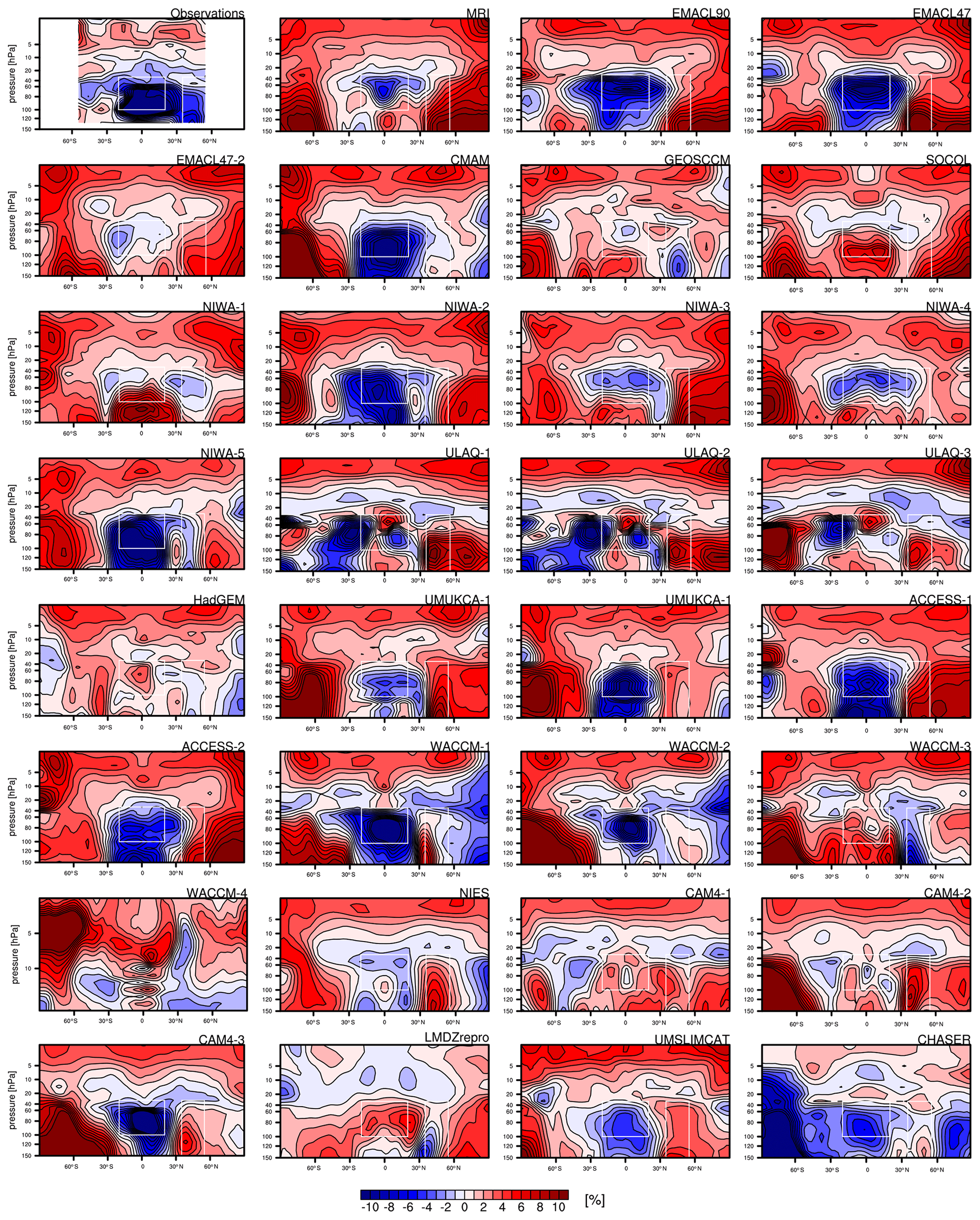
Figure 1Latitude–pressure cross-section of the relative ozone trend over the period 1998–2018 for the observational dataset BASICSG and for all CCMI REF-C2 simulations. Boxes illustrate the regions selected to integrate ozone in the LS for trend comparisons later in this study, i.e. in the tropics (20∘ N–20∘ S, 30–100 hPa) and in the northern mid-latitudes (30–50∘ N, 30–150 hPa).
The panels of Fig. 1 show a latitude–pressure cross-section of the ozone trend for observations (first panel of Fig. 1) and all free-running CCMI model simulations. Generally, the linear trend fit we perform on the BASICSG data yields similar spatial patterns and magnitudes to those estimated in Ball et al. (2018) with the DLM approach (see their Fig. 1f). There are a few small differences; e.g. our linear trend fit results in larger positive trends in the upper stratosphere over the southern tropics of ∼1 %, a slightly less negative trend in the Northern Hemisphere middle stratosphere (<1 %), and consistently large and negative trends close to 100 hPa in the tropics as opposed to a smaller and insignificant trend at around 10∘ S and over 100–80 hPa in the DLM estimate, as shown by Ball et al. (2019). Most notably, linear-trend calculations result in small positive trends (up to ∼3 %) in the southern mid-latitude lower stratosphere as opposed to overall negative but insignificant trends reported by Ball et al. (2019) in that region. However, the comparison reveals that the overall magnitude and trend pattern is also captured by the simple linear regression; i.e. it is not dependent on the exact method used to calculate the trends. Therefore, we proceed with using a linear fitting approach for the comparison between observations and CCMs, though the above caveats should be kept in mind when comparing with a full regression analysis using DLM (Ball et al., 2019).
Overall, large inter-model variability in the trends derived from the individual REF-C2 simulations (including all ensemble members) is revealed in Fig. 1. Nevertheless, a number of features can be identified that are consistent over most models and all their ensemble members. In the upper stratosphere (1–10 hPa) nearly all simulations consistently show an overall positive ozone trend. This ozone increase can be explained by the decrease in ODSs (see e.g. WMO, 2018) and by a slowdown in ozone destruction rates as the stratosphere cools from GHG increases (see e.g. Portmann and Solomon, 2007), as is further discussed in Sect. 3.5. This upper-stratospheric ozone trend has been found for climate model simulations and for observational data in several studies before (e.g. SPARC CCMVal, 2010; Harris et al., 2015; Steinbrecht et al., 2017; Ball et al., 2018, 2020; WMO, 2018). However, in the lower stratosphere (30–100 hPa in the tropics, 150 hPa in the mid-latitudes) we find a wide spread in the ozone trends among the CCM simulations over recent decades. Many REF-C2 simulations exhibit negative trends in the tropical LS, and they are comparable to the observational trend in magnitude and structure. In agreement with earlier studies (e.g. WMO, 2018; Orbe et al., 2020), we show in Sect. 3.4 that this tropical ozone decrease is related to enhanced tropical upwelling in a warmer climate. However, there are also simulations showing a positive LS ozone trend in the tropics (i.e. GEOSCCM, SOCOLv3, NIWA-1, WACCM-3/4, CAM4-1/2, LMDZrepro, HadGEM; note that the number of the ensemble run is denoted with −1, −2, and so on). At northern and southern mid- and high-latitudes most simulations exhibit a positive trend but with a pronounced inter-model spread. Only a few simulations show negative trends in either northern or southern mid-latitudes (e.g. GEOSCCM, WACCM-3, WACCM-4), but it is important to point out here that none of the 31 simulations reproduce the observed negative ozone trend pattern with an ozone decrease covering the tropical belt and extending to the mid-latitude (50∘ S–50∘ N), as shown in the upper left panel and previously in Ball et al. (2018, 2019). This discrepancy in the LS ozone trend between observations and models has been reported before (e.g. ozone trends, based on CCMI simulations (WMO, 2018; Orbe et al., 2020), and in comparison to CCMVal-2 simulations (Ball et al., 2020)). For CCMs that provide multiple ensemble members (WACCM, NIWA, ULAQ, ACCESS, CAM4, and UMUKCA), we also identify a large ensemble spread in the simulated LS ozone trends. For example in WACCM two ensemble members simulate positive tropical ozone trends, while the two other members simulate negative tropical ozone trends. In WACCM (as well as in NIWA and CAM4), the coupled ocean allows for differences in the SST variability between the ensemble members, possibly explaining the large spread in tropical ozone trends. However, as is also the case for models with prescribed SSTs (ACCESS, ULAQ, UMUKCA) that exhibit a large spread between the simulations, the SST variability is not the only reason for the different trend pattern, as was similarly reported and discussed by Ball et al. (2020) for CCMVal-2 models. The large spread in LS ozone trends between ensemble members is further in agreement with the study of Stone et al. (2018). They used a nine-member ensemble of a free-running CCM simulation (CESM1-WACCM) and showed that LS ozone trends over the years 1998–2016 are characterized by large internal variability, with, for example, the LS ozone trend ranging from +6 % to −6 % per decade. But note again that none of these ensemble members showed the coherent decrease in ozone in the tropics and extratropics as found in observations (Ball et al., 2020).
Following this qualitative discussion on the spread in the ozone trend pattern between the CCM simulations, we now turn to the LS ozone trends with a more quantitative comparison of the apparent inconsistencies between observations and CCMs. We calculate the trends of the deseasonalized LS ozone columns for the period 1998–2018 in two regions: the inner tropics (20∘ N–20∘ S) and in the northern mid-latitudes (30–50∘ N). We choose the northern mid-latitude band 30–50∘ N for direct comparability with the study of Ball et al. (2020). The pressure range of the lower stratosphere was taken to be 30–100 hPa for the tropics and 30–150 hPa for the mid-latitudes to take into account the differences in latitudinal tropopause heights. Trends and their uncertainties (represented by the 90 % confidence interval of the linear slope) are shown for each of the 31 available REF-C2 simulations of 18 different CCMs in Fig. 2. We decided to focus on the northern mid-latitudes here because the SH mid-latitude trends are likely more strongly influenced by the large chemical depletion of ozone within the polar vortex. We come back to the LS ozone trends of the southern mid-latitudes in Sect. 3.5.
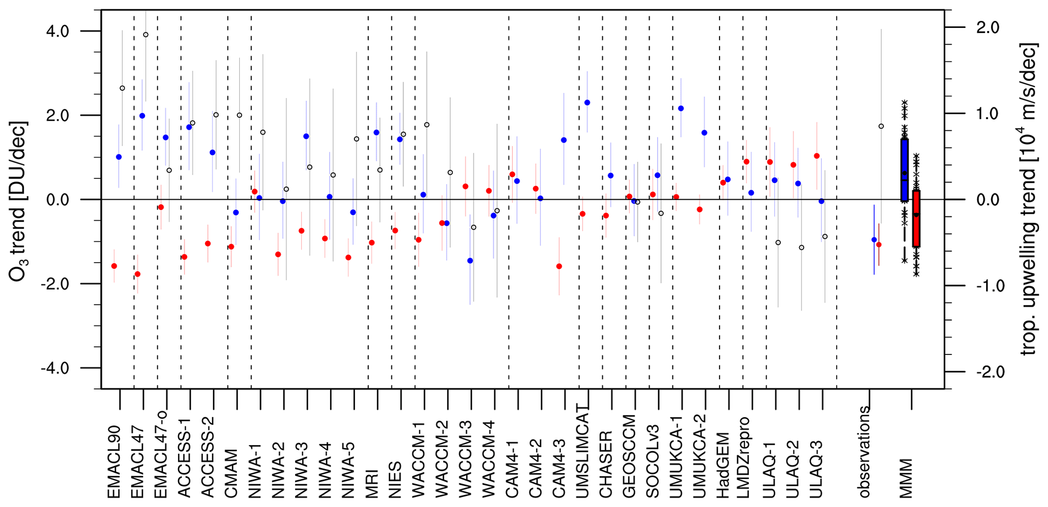
Figure 2LS ozone trends and their uncertainties in the tropics (20∘ N–20∘ S; red dots) and northern mid-latitudes (30–50∘ N; blue dots) together with tropical upwelling trend (black circles; for all simulations providing TEM diagnostics) for the period 1998–2018 for all REF-C2 simulations. Dashed lines separate the individual models. Moreover, observational trends (1998–2018) and multi-model mean trends are given. Observational data for ozone are taken from BASICSG and for tropical upwelling from ERA5 reanalysis. Error bars associated with each LS ozone trend represent the 90 % confidence intervals. The multi-model mean trends are shown as boxplots: the solid black line in the box indicates the median, the black point indicates the MMM, and the coloured box ranges from the 25th to the 75th percentile of the trends. Crosses denote trends of individual model simulations not lying within the box.
In the tropics about half (42 %) of the REF-C2 simulations show a significant decrease, about the same (42 %) show a non-significant change, and about 15 % show a significant increase in the integrated tropical LS ozone column. Note that significance is defined as the non-overlap of the error bars (90 % confidence interval) with the zero trend. The resulting MMM ozone trend (see red bar on right of Fig. 2) is negative (−0.37 DU per decade), but it is insignificant due to the considerable spread among the different models. The 25th–75th quantile of the distribution ranges from −1.12 to 0.20 DU per decade (see edges of box on the right of Fig. 2). Note that for the calculation of the MMM trend, we choose to weight each of the 31 simulations equally (i.e. not taking into account that some models have multiple ensemble members) because the trend variations among ensemble members are as large as among the different models over this period.
The observed tropical LS ozone trend of −1.07 DU per decade is statistically significant at the 90 % level. Thus the observed tropical trend is more strongly negative than the MMM trend but lies within the 90 % confidence interval of the MMM trend ([−1.76 DU per decade; 1.03 DU per decade]).
In the northern mid-latitudes less than half (40 %) of the REF-C2 simulations show an increase in the LS ozone column, while the remaining 60 % of the simulations show a non-significant change (either positive or negative). There is only one simulation (WACCM-3) that shows a significant decrease in the mid-latitude LS ozone column, and in this simulation the tropical ozone trend is positive (but not significant). The resulting MMM trend in the northern mid-latitudes is positive (+0.63 DU per decade) with a high inter-model spread: the 25th–75th quantile of the distribution ranges from −0.04 to 1.42 DU per decade. Note here that the observational trend (−0.96 DU per decade) lies outside the 90 % confidence interval of the MMM trend in the mid-latitudes ([−0.91 DU per decade; 2.16 DU per decade]).
Figure 2 also reveals that over the years 1998–2018 more than half of the model simulations have a dipole trend pattern in the LS ozone column; i.e. the sign of the tropical ozone trend is opposite to that in mid-latitudes. This trend pattern with negative LS ozone trends in the tropics and positive LS ozone trends in the northern mid-latitudes can be found for almost half the simulations (45 %), and a trend pattern with a positive ozone trend in the tropics and negative trend in the northern mid-latitudes is found in 13 % of the simulations. The remaining simulations do not show this dipole, but both have either a positive trend in the tropics and the mid-latitudes (29 %) or a negative trend in both tropics and mid-latitudes (13 %, i.e. three simulations, namely NIWA-5, CMAM, and WACCM-2). Only 3 out of 31 simulations simulate negative but non-significant trends both in the tropics and northern extratropics, and thus they show a similar behaviour to observations (see right of Fig. 2 and Ball et al., 2019). However, their zonal trend patterns (see Fig. 1) reveal that none of these three simulations reproduce the observed trend pattern with consistent negative trends from 50∘ S–50∘ N in the LS. Consequently it is important to keep in mind that the results of these (averaged) trends depend on the choice of the latitude–pressure box as the integration over a wider latitude band can lead to a cancellation of opposing trends.

Figure 3Inter-model correlation between tropical (20∘ S–20∘ N) and northern mid-latitude (30–50∘ N) LS ozone column trends, calculated over the period 1998–2018 for 31 CCMI REF-C2 simulations. All ensemble members of a particular model are shown in the same colour. The observational ozone trends (BASICSG) are included as a star.
Next, we analyse whether a systematic relationship between the LS tropical and mid-latitude trends exists in the CCM simulations. For this, the simulated northern mid-latitude LS ozone trends are plotted against the simulated tropical LS ozone trends over the time period 1998–2018 for all 31 REF-C2 simulations and for the observed dataset BASICSG in Fig. 3. As discussed above, in the LS the majority (45 %) of the models have a negative ozone trend in the tropics and a positive trend in the northern mid-latitudes. Moreover this illustration again highlights that the trends estimated from observational data are lying on the outer edge of the model trend distribution. The inter-model correlation between the tropical to mid-latitude trends is negative with a low correlation coefficient (−0.25). Thus, for the chosen period the tropical ozone trends are only weakly linked to mid-latitude ozone trends in the models. However, we expected that the two trends are highly (negatively) correlated as from our understanding increased tropical upwelling leads to decreased tropical ozone, and this upwelling increase should be linked to an increased mid-latitude downwelling, which would enhance ozone in the mid-latitudes. However Fig. 3 does not support this. Also slightly varying the period (i.e. looking at the periods 1999–2019, 2000–2020, and 2001–2021) reveals very low negative or near-zero correlations (not shown here). To get a better understanding of the processes leading to the given LS ozone trend patterns, we investigate the relationship of LS ozone trends to stratospheric transport trends in Sect. 3.4.
Overall we can conclude from the analysis of ozone trends in the suite of CCMI models (see Figs. 1–3) that the LS ozone trends exhibit a considerably large spread across both the different models but also across ensemble members from a single model, in particular in the mid-latitudes. This indicates that ozone variability considerably influences the LS trends, in agreement with the recent studies by Chipperfield et al. (2018) and Stone et al. (2018). However, even when considering the high variability in possible trends in CCM simulations, the observational trends emerge as an unlikely realization of the simulations over the period 1998–2018. In the next section, we analyse the robustness of this finding by varying the period of the trend calculation and providing an in-depth statistical analysis of the likelihood of the observed trend lying within the suite of modelled trends.
3.2 Robustness of lower-stratospheric ozone trends
In the previous section we found that the observed negative ozone trend in the LS mid-latitudes together with a simultaneous negative trend in the tropics is unlikely, based upon the suite of CCM simulations. To further establish the robustness of this result, we here test whether this also holds for time periods that are slightly different to the period 1998–2018 we considered before. Thus, in this section we first want to investigate how variability influences the ozone trends, and second we want to quantify the likelihood of the observed trend being a realization of the distribution of the modelled trends. To answer those questions, we calculate the LS ozone trends by varying the start and end years of the time period. In Fig. 4a and b, the observed tropical and mid-latitude ozone trend in the LS is shown for start years varying from 1995–2001 (y axes) and end years from 2013–2019 (x axes). Both tropical and mid-latitude LS ozone trends are consistently negative for all chosen periods in the observations (top row). This is in line with the results of Ball et al. (2019), who found that the observed negative sign of the tropical and mid-latitude trends remains insensitive to changing the end year. In the tropics, observational LS ozone trends are consistently negative, with values between −0.64 and −1.24 DU per decade for all possible start year–end year combinations. In the mid-latitudes the trends are also negative for all shown time periods but are more variable than in the tropics (values range between −0.11 and −1.22 DU per decade). In particular at mid-latitudes, the strongest negative trends are found for start years of 1996 to 1998, and a sudden decrease in the trend magnitude is found for the start years 1999 and 2000. Thus, the analysis in Ball et al. (2018, 2019) and in the preceding section focused on a period with particularly strong negative mid-latitude ozone trends. Possible reasons for the sudden change in the trend, such as the strong ENSO event in 1998, are discussed in Sect. 4. Note that the trend magnitude increases again for the start year 2001, which again suggests that interannual variability influences the observational mid-latitude trends.
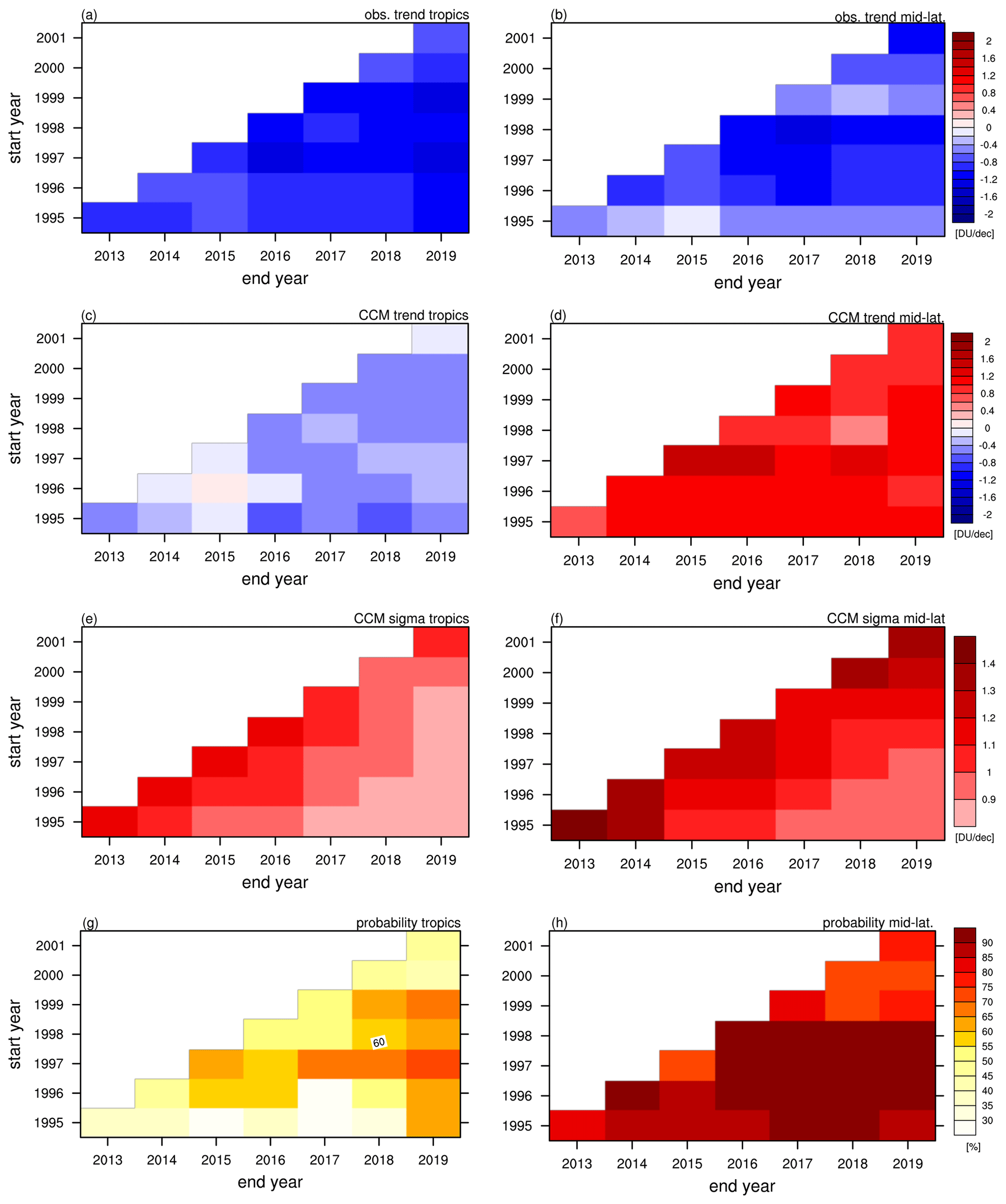
Figure 4Tropical (a, c, e, g) and mid-latitude (b, d, f, h) LS ozone trends (in DU per decade) as a function of different periods for the observational trend of BASICSG (a, b), the most likely trend of the modelled REF-C2 probability distribution (c, d), and the 1σ standard deviation (in DU per decade) of the mean obtained from the probability distribution (e, f). The panels (g) and (h) show the “probability of disagreement” (in per cent) between observed trends and the REF-C2 trend probability distribution. In all panels the x coordinate denotes the different end years (2013–2019) and the y coordinate the different start years (1995–2001).
Figure 4c and d display the tropical and mid-latitude trends as a function of start and end year derived from the model simulations. To do so, a robust estimate of the trend probability distribution considering all model simulations was derived (see Sect. 2.3), and from this distribution the most likely trend is shown (see peak in the models' trend probability distributions of Figs. S1 and S2 in the Supplement). In the tropics the ozone trends derived from the REF-C2 simulations are negative and range from −0.74 to +0.02 DU per decade. In the mid-latitudes the trends are positive for all possible start year–end year combinations, with values ranging from +0.4 to +1.48 DU per decade. In contrast to the sudden change in the mid-latitude observational trend for start years 1999 and 2000, in the REF-C2 simulations no such systematic change can be found. The estimated probability distributions of the trends from the REF-C2 simulations (see Figs. S1 and S2) are typically symmetric around their maximum value and show a single, central peak. The width of the distribution changes when varying the start year–end year combination, with narrower distributions for longer time periods. Moreover, visual inspection of the distribution implies that the tropics (Fig. S1) generally have Gaussian-like distributions, whereas the mid-latitudes (Fig. S2) often show a more peaked structure, i.e. with heavier tails. Nevertheless, as an estimate of the width of the models' trend distribution, we show in Fig. 4e and f the standard deviation of the models' distribution (in DU per decade) in the tropics and mid-latitudes, respectively. For longer time periods (values in lower right corner) the standard deviation of the models' trend is smaller; i.e. the distribution is narrower. This indicates that the influence of natural variability is less important for longer time periods, as should be expected.
Given the distributions representing the combined trends of the models, we can now quantify the disagreement between the observational trend estimate and the models' trend probability distributions for each start year–end year combination. In Fig. 4g and h the “probability of the disagreement” between observational and modelled LS ozone trends is given for the tropics and the mid-latitudes. The value of the “probability of disagreement” is calculated by the central interval of the models' probability distribution when taking the observed trend value as the threshold of this interval. Thus, a probability value of 90 % indicates that the observed trend falls within the inner 90 % of the distribution; i.e. only 10 % of the distribution is more extreme than the observed trend: the smaller the given “probability of disagreement” value, the higher the probability that the observed trend lies within the models' distribution. In the tropics, the observed LS ozone trend falls within the 13 %–73 % interval of the modelled probability distribution; i.e. the observed trends are generally likely representations of the models' trends. The agreement is best for short time periods (values in diagonal in Fig. 4g), mostly because of the broader distribution (see Figs. 4e and S1). Also for early start years (in particular 1995) and end years ranging from 2013 to 2018, the disagreement is small because model trends are strongly negative for this period (see Fig. 4c). In the mid-latitudes, the observed trend generally lies at more distant parts of the models' trends distribution (73 % to 96 %); i.e. the observed trend is a more extreme value in the models' distribution. The disagreement is smallest for both the earlier periods (lower left; start years 1995–1997 and end years 2013–2015) and the later periods (upper right; start years 1999–2001 and end years 2017–2019). This coincides with the generally smaller negative trends in those periods in observations (see Fig. 4b) and rather constant trend distributions in the models (see Fig. 4d). For the periods with the strongest negative observed trend (start years 1996–1998), the observed trend lies within the central 90 % or higher of the models' distribution, i.e. is an unlikely representation from the modelled trends. The sudden decrease in the observed trend magnitude for start year 1999 (Fig. 4b) is reflected by a decrease in the central interval to about 75 %. In general, one might have expected that longer periods lead to better agreement of the observed and modelled trend due to the smaller influence of variability (see Fig. 4e and f) – as we do in the models – however, we do not find this to be true for either the tropics or the mid-latitudes.
3.3 Convergence of future lower-stratospheric ozone trends
In the previous section, the ozone trend robustness was analysed for time periods of up to 25 years. We show in the following that, as the considered time periods are extended, the influence of natural variability decreases, and the trends converge to the trend forced by long-term GHG and ODS concentration changes. To analyse the timing and the values of the trends' convergence, we extend the period for the trend calculation into the future for all REF-C2 simulations.
.

Figure 5Tropical (20∘ S–20∘ N) and northern mid-latitude (30–50∘ N) LS ozone column trend and their uncertainties (in DU per decade) of observations (BASICSG) and REF-C2 simulations as a function of the end year (red and blue dots, respectively). Tropical upwelling trends are included for all REF-C2 simulations where TEM diagnostics were available (black dots); observational tropical upwelling is taken from ERA5 reanalysis. The end year varies from 2013 to 2019 for observational data and from 2013 to 2060 for REF-C2 simulations. Error bars associated with each trend represent the 90 % confidence intervals.
Figure 5 shows the tropical and northern mid-latitude LS ozone trends together with the tropical upwelling trend (black) for periods with the fixed start year 1998 and the end year varying from 2013 up to 2060 by extending the time period by steps of 1 year. For reference, the observational trends of ozone (from BASICSG) and tropical upwelling (from ERA5) are shown in the upper left panel of Fig. 5, with the last available end point in the year 2019. As shown in the last section, the trends derived from observational data are consistently negative both in the tropics and in the northern mid-latitudes.
As discussed in Sect. 3.1, the ozone trends exhibit a strong inter-model spread for the observational time periods. Both tropical and mid-latitude ozone trends in the individual model simulations vary considerably for different end point years within the observational period (left of the vertical dashed grey lines). The northern mid-latitude trend is generally more variable than the tropical trend. For longer time periods extending into the future, the uncertainties in the LS ozone trends decline, and the trends converge in all simulations. All model simulations consistently simulate persistent negative or near-zero trends in the tropics and positive or near-zero trends in the northern mid-latitudes. However, the timing of convergence of the trends to this trend pattern is rather different in the simulations, as can be inferred from Fig. 5; i.e. the convergence appears to be model-dependent. For some models, the trends vary little for end years after 2020 (e.g. MRI in Fig. 5), while in other models, the trends still vary considerably until end years around 2030 to 2040 (e.g. the four WACCM ensemble members in Fig. 5). The timing of the convergence is controlled by the ratio of the year-to-year variability to the strength of the forced trends. The relative forcing by ODS versus GHG changes over time, and thereby the forced ozone trends vary over the time periods as well, making it difficult to quantify an exact date of convergence. Still, the trend estimates for the entire period 1998 to 2060 do converge to stable values for almost all models, thus representing the forced trend for this time period. The trend magnitudes over this long period vary strongly between the models, from −0.10 to −1.32 DU per decade in the tropics and from +0.39 to +2.00 DU per decade in the mid-latitudes. Comparing this to the model range of the shorter time period 1998–2040, we see that the tropical trend (+0.06 to −1.12 DU per decade) has not converged to the end point values of 2060 yet. The mid-latitude trend (+0.54 to +2.15 DU per decade) is however close to the 2060 values.
Overall, the mid-latitude trends converge to positive values in the majority of the model simulations (about 85 %) by 2030. Thus, if both the year-to-year variability and the forced response of the models is simulated realistically, we should expect the emergence of positive mid-latitude trends from observational records within the next decade.
3.4 Influence of transport processes on LS ozone trends
In this section we aim to improve our understanding of how transport processes control the LS ozone trends in the models. As is well known from earlier studies, tropical upwelling significantly influences stratospheric ozone in the tropics (e.g. Oman et al., 2010). Enhanced tropical upwelling leads to more transport of tropospheric ozone-poor air into the tropical LS. Moreover, a faster removal of ozone in the tropical pipe reduces the residence time in the LS. To analyse how tropical and mid-latitude LS ozone trends are influenced by transport processes, we show in Fig. 2 the tropical upwelling trends (20∘ N–20∘ S, 70 hPa) for all simulations providing TEM diagnostics. This shows that models with strong positive tropical upwelling trends also have large negative tropical ozone trends. However, for the mid-latitude trend it is difficult to visually detect a clear relation with tropical upwelling trends.
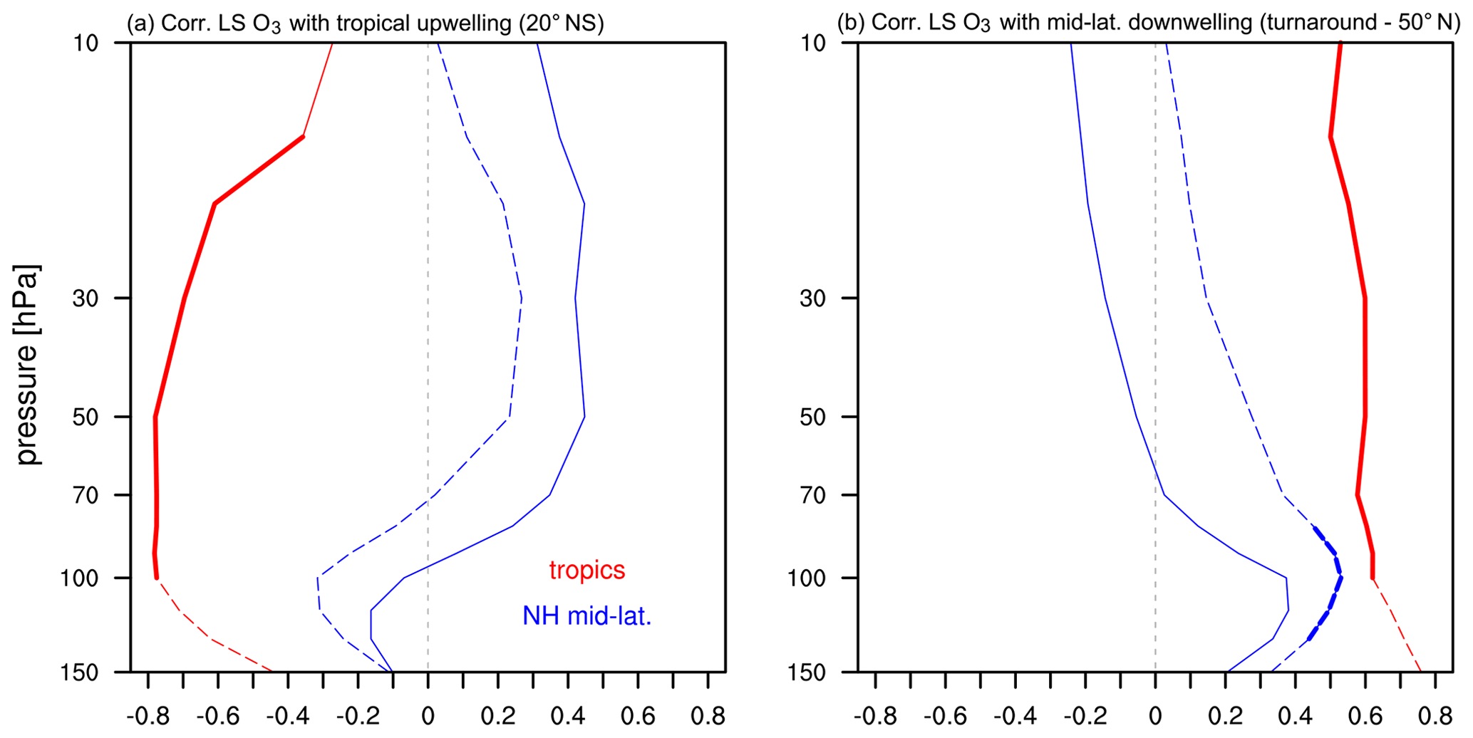
Figure 6Vertical profile of the inter-model correlation coefficients for (a) tropical upwelling (20∘ N–20∘ S) trends (kg s−1 per decade) to tropical (red line) and northern mid-latitude (blue line) LS ozone column trends and for (b) mid-latitude downwelling mass flux (between the turnaround latitudes and 50∘ N) trends (kg s−1 per decade) to tropical and northern mid-latitude LS ozone column trends. Correlations are calculated for upwelling and downwelling trends between 10 and 150 hPa. Mid-latitude ozone trends are averaged over the latitude band of 30–50∘ N (solid blue line) and also over the dynamically defined latitude band between the turnaround latitudes to 50∘ N (dashed blue line). Trends are calculated over the period 1998–2018 for a subset of 20 REF-C2 simulations. Correlation coefficients which are significant on the 95 % level are highlighted in bold.
Therefore we analyse the relation of tropical upwelling and extratropical downwelling trends to LS ozone trends in terms of a correlation analysis. Figure 6a shows the inter-model correlation between the tropical upwelling mass flux trends at different stratospheric levels and tropical LS ozone column trends over a subset of 20 REF-C2 simulations. Additionally the correlation of the northern mid-latitude downwelling mass flux trends at different levels and LS ozone column trends is provided in Fig. 6b. As above we calculate the trends over the period 1998–2018, and tropical ozone trends are averaged over 20∘ N–20∘ S and mid-latitude ozone trends over 30–50∘ N.
The correlation profiles between tropical ozone column trends and tropical upwelling trends (red line in Fig. 6a) show significant high negative correlations () at all levels between 30 and 100 hPa. Thus, as expected, changes in tropical upwelling at all levels below 30 hPa highly influence LS tropical ozone. This is in line with previous studies (e.g. Oman et al., 2010; SPARC CCMVal, 2010). Between 10 and 30 hPa, the correlation decreases with altitude and becomes insignificant. The correlation values of tropical ozone trends to downwelling trends are positive and also rather high (Fig. 6b). This is clear as upwelling is directly linked to downwelling; however the negative sign of downwelling causes a sign reversal of the correlation coefficients.
For ozone trends in the northern mid-latitudes (30–50∘ N), the correlation of LS ozone to tropical upwelling trends varies in altitude from about −0.2 to +0.4 (solid blue lines in Fig. 6a): it is weakly negative up to 100 hPa; above, the correlation turns to positive values (r≈0.4 at 70 hPa). Compared to the relation of upwelling trends to tropical ozone trends, these correlations are quite low and not significant at the 95 % level; moreover these correlations are not robust when slightly varying the period (not shown). The same is true for correlations between mid-latitude ozone trends and downwelling trends (see solid blue lines in Fig. 6b). A possible reason for the non-robust and non-significant correlations might be the choice of the mid-latitude averaging region from 30–50∘ N. This region can partly include regions of upwelling at some pressure levels, and the location of the turnaround latitude is model-dependent. Not accounting for a dynamically consistent averaging region might obscure the correlation analysis. Therefore, we additionally define a dynamically more consistent mid-latitude region by averaging the LS ozone column from the turnaround latitudes of the BDC to 50∘ N. For each month the averages were taken by calculating the position of the residual stream function maximum at each level and then averaging the LS ozone column from this turnaround latitude to 50∘ N. It was further ensured that tropospheric air is not included in the averages (which could happen at levels below the tropical tropopause) by using only the region above the tropopause.
Table 2MMM and observational ozone trends, calculated over the period 1998–2018 for tropical upwelling at 70 and 100 hPa, for extratropical downwelling at 70 and 100 hPa, for the LS tropical ozone column, and for the northern mid-latitude ozone column. Note that LS mid-latitude ozone trends are averaged over the fixed latitude band of 30–50∘ N and also over the dynamically defined latitude band between the turnaround latitudes to 50∘ N. MMM trends and their standard deviation are given over a subset of 20 REF-C2 simulations. Observation-based data for up- and downwelling are taken from ERA5 reanalysis and observational data for ozone from BASICSG.
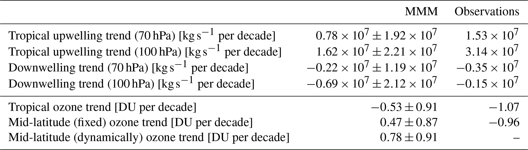
The ozone trends in this dynamically defined box are slightly higher compared to the fixed latitudinal region between 30 and 50∘ N, but given the large spread in trends this difference is not significant (see Table 2; the same is true for the longer period 1998–2040, not shown). The correlation profiles for LS ozone trends within this dynamically defined mid-latitude box are included in Fig. 6a and b (see dashed blue line): due to the dynamical consistency of mid-latitude ozone and the downwelling region, the correlations increase in absolute number compared to the correlations with ozone trends in the fixed boxes, and the correlations are more robust across different periods (not shown). In particular, the correlation of ozone trends in the dynamically defined averaging box to downwelling peaks at 100 hPa, with a significant correlation coefficient (r≈0.5). Up- and downwelling at around 100 hPa reflects the shallow branch of the BDC (see e.g. Abalos et al., 2014; Dietmüller et al., 2018). Thus, the significant positive correlation of downwelling trends around this level to mid-latitude ozone trends suggests that an enhanced shallow branch leads to a decrease in ozone in this region. This would be consistent with enhanced horizontal advection via the shallow branch that transports tropical ozone-poor air to the mid-latitudes. The fact that correlations decrease to insignificant correlation values above (and correlations to tropical upwelling even change sign) likely reflects the relation of mid-latitude ozone trends to downward transport of ozone via the deep branch. Thus, overall the correlation analysis suggests that the two competing transport processes of shallow horizontal versus deep vertical advection influence ozone in the mid-latitude LS.
In general, the weaker correlations of mid-latitude ozone to up- and downwelling compared to tropical ozone suggest that mid-latitude ozone changes are controlled by a variety of processes, possibly also including two-way mixing. Furthermore, changes in not only the transport strength but also in the background ozone gradients can lead to changes in the transport of ozone. For example, the increase in upper-stratospheric ozone mixing ratios could lead to enhanced downward transport of ozone despite an unchanged downwelling strength.

Figure 7Inter-model correlation coefficients between local ozone trends and (a) local AoA trends, (b) local RCTT trends, and (c) local AbM trends. Trends are calculated over the period 1998–2018 for a subset of nine REF-C2 model simulations. White contours show the MMM ozone climatology, and the stippled regions mark where correlation coefficients are significant on the 95 % level.
To better elucidate the role of different transport processes in the different regions, we additionally analyse the local correlation of AoA trends to the ozone trends for a subset of nine REF-C2 simulations that provide the necessary diagnostics (namely EMAC-L90, EMAC-L47-1, ACCESS-1, WACCM-1, CMAM, GEOS, SOCOL, MRI, NIWA-1). As shown in Fig. 7a, in the middle stratosphere the correlation coefficients are relatively weak, consistent with the expectation that chemical processes play an important role there. In the LS, we find very high correlations (larger than 0.8) between ozone and AoA trends in the tropics and extending to about 40∘ N. Thus, inter-model differences in ozone trends are highly controlled by differences in transport trends in this region. Negative correlation values can be found in the LS mid-latitudes north of about 40∘ N and above 80 to 60 hPa. Interestingly, in the SH correlations are positive throughout the LS. To analyse the role of different transport processes, we separate AoA into the components RCTT and AbM (for details see Sect. 2.4). The inter-model correlations between ozone trends and RCTT and AbM trends, respectively, are shown in Fig. 7b and c. In the LS, RCTT trends are highly positively correlated to ozone trends between 40∘ S–40∘ N, whereas for latitudes poleward of 40∘ the correlation coefficients turn to negative values. AbM trends and ozone trends correlate strongly (and positively) in the LS for latitudes poleward of 30∘. This again underlines that in the tropical LS residual transport changes largely control the ozone trends: negative RCTT trends (indicating faster upwelling) are associated with negative ozone trends. This is also in line with the findings of Fig. 6a. In the LS mid-latitudes, on the other hand, both changes in residual transport (RCTTs) and in mixing (AbM) have an impact on ozone trends, leading to the non-homogeneous correlation structure with AoA trends (Fig. 7a). In the region of our interest, i.e. 30–50∘ N, the different transport processes of residual transport with its deep and shallow branch and of two-way mixing appear to influence ozone trends: the RCTT correlations (Fig. 7b) suggest that an enhancement of the meridional component of the residual circulation (shallow branch) leads to an ozone decrease up to 40∘ N by enhanced transport of tropical ozone-poor air to the mid-latitudes. This is in line with the significant positive correlation of models' LS ozone and downwelling trends that we presented in Fig. 6b. The negative correlations between RCTT and ozone trends north of 40∘ N indicate that ozone trends are driven by vertical downwelling (from the deep branch) here: enhanced downwelling (lower transit time) is associated with transport of ozone-rich air from above. Moreover mixing processes play a role in the mid-latitude region. The correlation of AbM trends with ozone trends is positive (r≈0.6) north of 30∘ N in the LS, indicating that mixing is strongly influencing ozone trends in this region as well. Overall Fig. 7 reveals that transport processes in the LS mid-latitudes are complex as this region is influenced by many competing transport processes. We discuss this issue further in Sect. 4.
3.5 Forced ozone trends in models
In the previous sections we analysed the ozone trends of the recent 20-year period in detail and found that modelled and observed ozone trends disagree, especially in the northern mid-latitude LS. Assuming the observational data are correct, the question that arises from our results is whether the disagreement stems from the influence of natural variability or whether the forced response to GHG or ODS concentrations is not captured correctly in the models. Thus in the following, we investigate the relative role of GHG versus ODS forcing in the ozone trends in the models for the observational period and periods extending into the future. Figure 8a and b show upper- and lower-stratosphere MMM ozone trends in the tropics (20∘ N–20∘ S), in the northern mid-latitudes (30–50∘ N), and in the southern mid-latitudes (30–50∘ S) for the REF-C2 simulations as well as for the sensitivity simulations with fixed ODS (fODS) and with fixed GHG (fGHG) concentrations (for a detailed description of these sensitivity simulations see Sect. 2.1). These MMM ozone trends are calculated for the recent time period (1998–2018), for a time period which extends into the future (1998–2040), and for a future time period (2050–2100). We also include the respective observational trends for 1998–2018. Note that for the calculation of the MMM trends only 10 model simulations are taken into account as the fODS and fGHG simulations are not as numerous as the REF-C2 simulations (see Table 1). Moreover we exclude ULAQ for the MMM calculation as its values are clear outliers compared to other models such that it would shift the MMM to lower absolute values. Note further that the MMM ozone trends are calculated as the average of the ensemble-means from each model. This ensures that models are weighted equally regardless of their ensemble size, which is desirable here as we aim to extract the forced trends, in particular for the longer time periods. Next to the trends averaged over the tropics and mid-latitudes, Fig. 9 shows the latitudinal distribution of the ozone column trends in the upper and lower stratosphere over the period 1998–2040 for the REF-C2, fODS, and fGHG simulations. Note that we show the trend over the period 1998–2040 here as we expect the forced signal to emerge more clearly for this period compared to the shorter observational period.

Figure 8MMM ozone column trends in the tropics (red; 20∘ N–20∘ S), in the northern mid-latitudes (blue; 30–50∘ N), and in the southern mid-latitudes (cyan; 30–50∘ S) for thee different periods (i.e. 1998–2018, 1998–2040, 2050–2100) for (a) the upper stratosphere (1–10 hPa) and (b) the LS (30–100 hPa in the tropics, 150 hPa in the mid-latitudes). The boxes extend from the lower to upper quartile of the data, with a line for the median and with whiskers to show the minimum and maximum values of the LS MMM ozone trends. MMM trends are given for REF-C2 simulations (filled boxes) as well as for fGHG and fODS simulations (not-filled boxes). Note here that for the estimate of MMM trends only 10 model simulations are taken into account as this is the maximum of available fGHG simulations, and we want to ensure that all three simulation types include the same models for the MMM trend estimate. Individual model trends are denoted by black stars for REF-C2, by black pluses for fGHG, and by black crosses for fODS. Observational data are included for the trends over the period 1998–2018 (red, blue, and cyan points, respectively).
In the upper stratosphere, the MMM ozone trends over the periods 1998–2018 and 1998–2040 are positive and of the same magnitude in tropical and mid-latitude regions (Fig. 8a). The 1998–2018 MMM trends are more than twice as strong as the observed trends (dots in Fig. 8a), with only one model simulation having lower trend values (in the tropics and NH). Even for the short period of 20 years, the ozone trends are consistently positive for both the models and the observations, indicating that the upper-stratosphere MMM trend is robust to interannual variability. Therefore, this likely is the forced signal driven by GHG and ODS changes. The analysis of the models' latitudinal distribution in upper-stratospheric ozone column trends shows no considerable latitudinal variation (see Fig. 9a). The positive upper-stratospheric MMM trend can be explained by the combined effect of still-decreasing ODS concentrations at the beginning of the trend periods 1998–2018 and 1998–2040 and by rising GHG concentrations causing stratospheric cooling. The contribution of these two effects is quantified by comparing fGHG, fODS, and REF-C2 simulations. In fGHG, the GHG-driven increase in the stratospheric circulation (resulting mostly from the increase in SSTs) as well as GHG-induced stratospheric cooling is excluded. In fODS, the chemical ozone destruction via ODS concentrations is excluded. Upper-stratospheric ozone trends in fGHG and fODS are positive but considerably lower than in REF-C2, with trends in fODS having the lowest values. This is in particular true for the extended period 1998–2040, where we expect clearly forced trends. The weaker upper-stratospheric ozone trend in the fGHG simulations can be explained by the missing additional ozone increase due to GHG-induced stratospheric cooling as ozone is photochemically controlled in these upper regions. The weaker trend in the fODS simulations can be explained by the missing additional increase via the recovery from ODS destruction. The comparison of fODS and fGHG trends over the period 1998–2040 reveals that about two-thirds of the REF-C2 upper-stratospheric trend is due to the ODS-forced trend. The upper-stratospheric trends over the second half of the century (2050–2100) reveal that the ceasing influence of ODS forcing manifests in decreasing ozone trends in the fGHG simulations. However, the ODS forcing still contributes to the ozone increase by about as much as the GHG forcing.
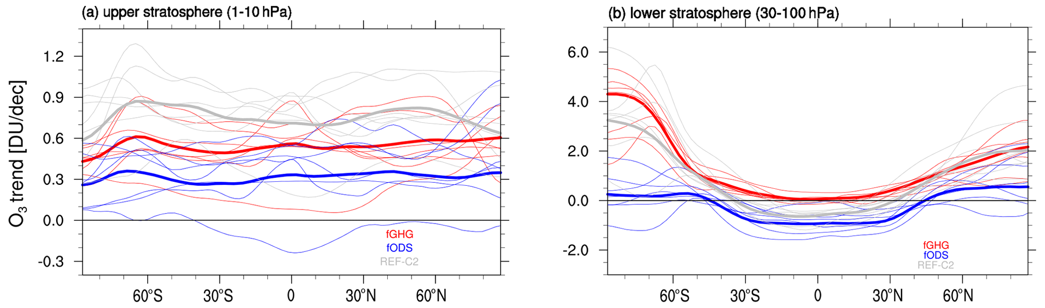
Figure 9Latitudinal distribution of ozone column trends over the period 1998–2040 for all REF-C2 (grey lines), fGHG (red lines), and fODS simulations (blue lines) for (a) the upper stratosphere (1–10 hPa) and (b) the LS (30–100 hPa). Thick lines indicate the MMM ozone trends.
For the LS, Fig. 8b highlights that ozone trends are highly variable in particular for the shorter period of about 20 years and that the MMM ozone trends over the period 1998–2018 and 1998–2040 are negative in the tropics and positive in the mid-latitudes in the REF-C2 simulations. In general, the mid-latitude ozone trends are very variable both in the northern and southern mid-latitudes, but the southern mid-latitude trends are somewhat lower (and negative in some models) for the shorter period. Also in observations, the SH mid-latitude trend is more uncertain and variable (compare observational estimates in Fig. 8b; see also Ball et al., 2019).
In order to attribute modelled LS ozone trends to GHG and ODS changes, we compare the ozone trends of the REF-C2 to fGHG and fODS simulations in Fig. 9b (see also MMM trends in Table S1 of the Supplement). For the short time period of about 20 years we find that the MMM mid-latitude ozone trends are positive and overall similar between the fGHG and the REF-C2 simulations. The fODS simulations, in contrast, show a negative MMM mid-latitude trend but with a very high inter-model spread. Compared to the REF-C2 simulations, the tropical LS trends are less negative in the fGHG simulations and more negative in the fODS simulations. This is what we expect from the missing influence of the GHG concentration rise on tropical upwelling. But note that trends of fODS, and fGHG are not significantly different from the REF-C2 simulation. The small, mostly non-significant differences (not shown) with their high inter-model spread in the fGHG, fODS and REF-C2 trends over the quite short observational period (1998–2018) again underlines the conclusion that variability strongly impacts LS ozone trends.
For the longer time period (1998–2040), the MMM fGHG trend in the tropical LS is near zero (see Fig. 8b and Table S1). In contrast to the trends over the short time period (1998–2018), the MMM fGHG trend can be clearly distinguished from the negative REF-C2 trend and also from the negative MMM fODS trend, which is comparable to the REF-C2 trend. This can be explained by the absence of GHG-induced enhancement of tropical upwelling, which strongly influences tropical LS ozone trends. The latitudinal distribution in Fig. 9b shows in more detail the tropical LS ozone column trends in the individual fGHG simulations (thin red lines): most models show trends near zero in the tropical region. The slightly negative ozone trends in the tropics in two models are a bit surprising. However, they probably can be explained by the fact that the upper-stratospheric ozone increase can reduce the UV radiation reaching the LS, and thus less ozone is produced there chemically (see e.g. Meul et al., 2014). In the mid-latitudes, the MMM trend in the fGHG simulations is positive and only slightly smaller than the REF-C2 trend, whereas the fODS MMM trend is near zero (see Fig. 8b). This indicates that enhanced downwelling associated with the strengthened circulation plays a minor role in this selected region and is consequently not responsible for the positive trend found in REF-C2. This weak influence of downwelling trends on mid-latitude ozone trends is consistent with the results presented in Sect. 3.4. There, we found that downwelling mass flux via the deep branch and mid-latitude ozone trends are only weakly related in REF-C2. Moreover, the near-zero ozone trend in the fODS simulations underlines that the mid-latitude ozone trends are strongly influenced by ODS recovery. This might be through decreased local ozone destruction (as ODSs are still decreasing), or through ozone transport from upper or polar regions, where ozone is increasing strongly because of the “closure of the ozone hole”. Thus, ozone increases in the mid-latitudes, even without an enhanced transport circulation.
To better understand the fact that the mid-latitude fODS trend is near zero, although we expect transport-induced changes in the LS, we show in Fig. 9 (thick blue line) the latitudinal distribution of the MMM fODS LS ozone partial-column trend. Here we see that the LS mid-latitude band between 30–50∘ N lies just within a region where ozone trends are shifting from negative to positive values. The MMM trend is negative between 30–40∘ N and positive between 40–50∘ N, explaining the near-zero mid-latitude trend over the total latitude band. We suppose that the negative trend 30–40∘ N can be explained by enhanced advection through the shallow branch and/or two-way mixing and the positive trend between 40–50∘ N by enhanced downwelling, as suggested by the correlations with RCTTs (Fig. 7b). However, the individual models show quite noisy behaviour in the latitudinal distribution of LS mid-latitude ozone trends, mainly in the NH (thin blue lines in Fig. 9b), indicating that the relative role of trends in the different transport processes might differ in models. The trends in the fGHG simulations are near zero in the inner tropics and positive at all other latitudes, indicating that the recovery from ODSs leads to an increase in ozone almost everywhere throughout the LS. The latitudinal distributions thus indicate that the GHG-driven circulation changes would induce a decrease in ozone from the tropics up to 40∘ N and 40∘ S (leading to a near-zero trend in the region 30–50∘ N), but due to the recovery of ozone from ODSs, the trend is essentially shifted to positive values so that the average trend over 30–50∘ N is positive.
The LS ozone trends calculated over the period 2050–2100 confirm the role of ODSs in influencing the mid-latitude ozone trends: despite a strong increase in tropical upwelling in this period (not shown), which drives the strong decrease in tropical ozone in the REF-C2 and likewise the fODS simulations, mid-latitude MMM ozone trends are essentially zero (or slightly negative in the NH) in the fGHG simulation. The effects of an ODS recovery on mid-latitude ozone are smaller in this period due to the declining influence of ODSs, but in the SH mid-latitudes this still leads to a robust positive ozone trend.
Overall our analysis of the fODS and fGHG simulations suggests that the recovery from ODSs is a dominant player for LS mid-latitude ozone trends. GHG-induced circulation strengthening also impacts LS mid-latitude ozone trends, but the competing transport effects via shallow and deep branches lead only to small transport-induced trends when averaged over the region from 30–50∘ N.
In the previous sections we analysed ozone trends over periods spanning the past 2 decades (i.e. 1998–2018) in detail. We found that modelled and observational ozone trends agree well in the tropical lower stratosphere, but in the northern mid-latitude LS the observed ozone trend represents an extreme value in the distribution of model trends.
In the following, possible reasons for the discrepancy between the mid-latitude ozone trends in the model simulations and the observations are discussed. One possible reason for the disagreement between modelled and observed LS ozone trends could be issues with the satellite records. For example, instrument biases and drifts can lead to large uncertainties in the observations, particularly in the lower stratosphere. The effect can manifest as steps in the data when instruments which have different vertical resolutions are added that can influence trend estimates. For a thorough discussion on this topic, see Harris et al. (2015),Ball et al. (2017), and Petropavlovskikh et al. (2019). However, for the sake of this discussion we assume that the observational data record is correct. Hence, the question that arises from our results is whether the disagreement stems from the influence of natural variability or whether it is related to the forced trend, or more specifically the following can be said:
-
The mean value of the modelled trend distributions might be incorrect. In other words, the forced trend might not be captured correctly by the models.
-
If we assume that modelled trend distributions are correct, the observed ozone trend as an unlikely representation might emerge due to very anomalous conditions during the considered periods. This may be caused by extrema in natural variability in the beginning of the time series (late 1990s) and/or in the end of the time series (late 2010s).
-
The modelled trend distribution constructed from the REF-C2 simulations might be biased because natural variability (e.g. QBO and ENSO) is not represented adequately in the models. This could lead to an overly narrow trend distribution and thus would make the observed trend seem more unlikely than it is.
While it is not easily possible to test which of the above explanations is correct, in the following we discuss their possible contributions to the diagnosed disagreement in light of our results and what is known from the literature.
4.1 Representation of forced trends
Based on the CCMI-1 data, we confirmed previous studies in that the decrease in tropical LS ozone is strongly related to the GHG-driven increase in tropical upwelling. The tropical upwelling trend derived from reanalysis (ERA5) lies in the range of the upwelling trends simulated by the models but on the upper end of the range. This is consistent with tropical ozone trends, which are on the stronger (more negative) end of the trend range simulated by the models as well. Circulation trends derived from reanalysis bear considerable uncertainty (e.g. Abalos et al., 2015); however reanalyses tend to agree better in the recent decades (Thomas Birner, personal communication, 2018, S-RIP report). Therefore, the upwelling trend derived over the period 1998–2018 from ERA5 is likely better constrained compared to earlier periods.
In the mid-latitudes (30–50∘ N), we find that the GHG-driven circulation changes do not lead to a net trend in ozone. This is evident from the fODS simulations (see Sect. 3.5) and from the vanishing mid-latitude LS ozone trends over the period 2050–2100, when the influence of ODSs ceases. The correlation analysis in Sect. 3.4 revealed that competing processes influence ozone trends in this region: an enhanced shallow branch in the LS can decrease ozone due to enhanced horizontal advection, while enhanced downwelling in the deep branch increases ozone (see correlation to RCTTs; Fig. 7b). In the fODS simulations, those competing influences lead to negative LS ozone trends equatorward of 40∘ N and 40∘ S and to positive ozone trends poleward 40∘ N and 40∘ S (see Fig. 9). Thus, this leads to nearly vanishing ozone trends in the mid-latitude region defined as 30–50∘ N. The consistent simulation of positive ozone trends in the mid-latitude LS in the REF-C2 MMM for the recent past and the coming decades is thus a result of the ODS concentration decline rather than of GHG-driven circulation changes. The effects of declining ODS concentrations on LS mid-latitude ozone can be related to either the chemical recovery of ozone, leading to local increases in ozone, or maybe more importantly to enhanced ozone transport into this region. Another effect can be induced by the circulation changes due to ODS-driven ozone changes that have been shown to have had a strong impact on AoA trends in the past (Polvani et al., 2019; Abalos et al., 2019). However, future circulation changes due to this effect are shown to be weak (Polvani et al., 2019). Furthermore, ozone-induced circulation changes are stronger in the SH, not consistent with approximately symmetric ozone trends in the mid-latitudes of both hemispheres.
Given that the positive mid-latitude ozone trends in models are driven by ODSs rather than by GHG changes, the discrepancy to the observed trend could indicate a mismatch in the relative role of the response of ozone to ODS versus GHG forcing. This means that either the GHG-driven circulation change in the models could be underestimated or differ in structure, or the ODS-driven ozone increase in the mid-latitude LS could be overestimated in the models. As for the latter, we showed that upper-stratospheric ozone increases more strongly in the models than in the observational data (see Fig. 8a). Thus, one hypothesis would be that the ODS-driven recovery of stratospheric ozone in the period since the late 1990s is generally overestimated in the models, which would then make negative ozone trends in the mid-latitude LS unlikely in the models. As for the effects of the GHG-driven circulation changes, we mentioned earlier that the MMM tropical upwelling trend is weaker compared to the estimate from ERA5 reanalysis (see Table 2). However, the generally consistent tropical ozone trends between models and observations rule out a vast underestimation of tropical upwelling changes. Rather, structural circulation trend differences could contribute to the disagreement in the mid-latitudes. An indication for these structural trend differences is the lower mid-latitude downwelling trend diagnosed from ERA5, which strongly differs from the model trends (see Table 2). This is also consistent with the finding of poleward-shifted turnaround latitudes by Orbe et al. (2020), as discussed below. While it is a likely explanation that structural circulation trends or anomalies contribute to the observed ozone trends, it is not easily possible to separate the role of natural variability in forming those structural circulation trends (see discussion on natural variability below).
In general, since LS mid-latitude ozone trends are driven by competing transport processes (see Sect. 3.4), the mismatch of trends in this region between models and observations might also indicate a misrepresentation of transport processes in the models. We show that ozone trends in the LS correlate well with trends in the passive AoA tracer, indicating that the differences in ozone trends between models are transport-driven. While there is a long-standing discrepancy of AoA trends derived from observations and models in the mid-stratosphere, AoA trends in the mid-latitude LS tend to agree well between models and observations (see e.g. Chapter 5 of WMO, 2018). On the other hand, climatological mean AoA in the suite of CCMI models used in this study varies considerably between models, and it was shown that this is due to differences in mixing effects on AoA (Dietmüller et al., 2018).
The studies of Wargan et al. (2018) and Ball et al. (2020) argue that the LS mid-latitude ozone decrease in observational data is possibly linked to enhanced two-way mixing. Ball et al. (2020) used effective diffusivity (Haynes and Shuckburgh, 2000) as a diagnostic for horizontal mixing and found that in reanalysis data (JRA-55, ERA-Interim) mixing is enhanced in the 1998–2018 period. In an earlier study, Ray et al. (2010) also showed a substantial increase in effective diffusivity under a changing climate for CCMs and reanalysis data (JRA-25, ERA-40). Recently, Orbe et al. (2020) used the TEM budget analysis of an idealized short-lived tracer (that covaries with ozone on interannual and decadal timescales) in 10 free-running ensemble member simulations with the GEOSCCM model in order to identify the mechanism that is driving the negative LS ozone trends. In contrast to the studies of Ball et al. (2019) and Wargan et al. (2018), the study by Orbe et al. (2020) showed that the mixing effect is not as important for the LS mid-latitude ozone trend. Rather they found a poleward expansion of the residual circulation in the LS with weaker downwelling in the sub-tropics and stronger downwelling in the mid-latitudes, leading to negative LS trends in the NH. However, as discussed in Orbe et al. (2020), mixing must be considered in the context of the specific tracer that is analysed (i.e. short-lived tracers are less sensitive to mixing). As such, the analysis of the TEM budget for the tracer ozone could be a focus in further investigations.
Overall, the LS ozone trends are strongly affected by variability over the short period, making it difficult to infer whether the forced trends in models and observations agree. For the models, we extended the time period into the future to investigate the period length for which the trends converge. We find that the inter-model spread of the ozone trends substantially diminishes for the longer time period (1998–2040) but to a different extent for different regions (see Fig. 8). In the upper stratosphere, MMM trends are significantly positive already for the shorter period 1998–2018. In the LS, the MMM ozone trends consistently show positive trends in the mid-latitudes for the period 1998–2040, with a comparably low inter-model spread. Thus the question arises as to whether we can expect observational data to also show a positive ozone trend in the mid-latitudes in the future. If the forced model trends are assumed to be correct, we should expect this positive trend to emerge by about 2030 to 2040 (compare Fig. 5).
4.2 Influence of natural variability on the observed trend
Sources of natural variability that strongly influence LS ozone are volcanic eruptions, the QBO, and ENSO. No major volcanic eruption occurred during the analysed period, so we disregard this source of variability. The influence of the QBO and ENSO on the hemispheric mean mid-latitude ozone is of the same magnitude, and thus they can both impact LS ozone trends, as shown by the study of Olsen et al. (2019).
We know from earlier studies that the QBO has a strong dynamical effect on the sub-tropical and mid-latitude LS ozone (e.g. Randel and Wu, 2007). Moreover it was recently shown that ozone trends in the mid-latitudes are directly linked to the QBO as the QBO induces a secondary circulation (see e.g. Ball et al., 2019 and Andrea Stenke, personal communication, EGU 2020). In 2016, the typical QBO phasing was disrupted, and this has been shown to be associated with negative LS ozone anomalies in the tropics (Kusuma et al., 2019). These negative anomalies at the end of the time period would lead to a strengthened negative ozone trend, and our analysis indeed shows slightly stronger negative tropical ozone trends for the end year 2016 compared to 2015 (see Fig. 4a). The mid-latitude ozone trend is also stronger for the end year 2016, which however does not fit expectations (QBO-induced anomalies are of a different sign in tropics and extratropics; see e.g. Randel and Wu, 2007). Another way in which the QBO could lead to decadal-scale variability in ozone and thus influence the trends was recently reported (Jessica Neu, personal communication, December 2018): since the QBO's influence on tropical upwelling depends on the season, the timing of the QBO phases is crucial for its influence on trace gas concentrations. Similarly, Ball et al. (2019) pointed out that non-linear attribution may be required to capture the QBO's impact.
One of the strongest warm ENSO events on record occurred in late 1997 (Jensen et al., 1998). By using CCM (WACCM) simulations with prescribed SSTs from observations, Calvo et al. (2010) showed that this strong ENSO event was associated with low ozone values in the tropics and high values in the mid-latitudes. This is in line with observational results by Randel et al. (2009). Consequently, mid-latitude ozone trends should be more negative when beginning the time period with this warm ENSO year. This is consistent with the strong mid-latitude trends in the BASICSG dataset for the start year 1998 (and less so for 1996–1997; see Fig. 4b). However, as the tropical trend is not associated with weaker negative trends for the start year 1998, this explanation is again not fully consistent.
As stated earlier, we have refrained from applying a multiple linear regression (MLR), which potentially would take at least part of the named sources of variability into account. If the trend strengths and patterns are strongly influenced by anomalous natural-variability events, one might argue that removing this variability via an MLR method would have a large impact on the trends. However, the trend estimates by Ball et al. (2018) that take ENSO and QBO variability into account differ only in details from the linear trend estimates. Note that an MLR method might not fully account for the induced signals by QBO or ENSO because, as mentioned above, their influence is likely non-linearly dependent on the signal strength and the signal timing. Thus, an MLR analysis cannot conclusively clarify the role of natural variability for the observed trends.
Overall, the sudden systematic change in the magnitude of the mid-latitude observational trend (Fig. 4b) indicates that natural variability (in particular the strong ENSO event in 1997) influenced the observed trends over the analysed periods and contributed to the particularly strong disagreement of observed and modelled mid-latitude trends for the relevant time periods. However, the expected effects of QBO and ENSO events on the trends are not entirely consistent between tropics and mid-latitudes. An exceptional combination of different factors possibly led up to the particular observed trend pattern, causing the mid-latitude trends to be more anomalous than the tropical trends in comparison to the trend distribution derived from the models.
4.3 Representation of natural variability in models
Above, we argued that natural variability likely influenced the observed ozone trends, and that might partly explain that trends over the observed period disagree with the trends in model simulations. However, how large this disagreement is depends on the underlying trend distribution derived from the models. For example, if the influence of natural variability is underestimated in the models, the trend distribution is too narrow.
The QBO is represented differently in the individual CCMs: some models generate a QBO internally, some models nudge winds towards a given QBO, and in some models the representation of the QBO is missing entirely (for more details see Morgenstern et al., 2017). Thus, over the whole suite of models, this could cause an underestimation of ozone variability in the models and therewith consequently a too narrow trend distribution. Moreover, as the QBO signal is treated differently across the REF-C2 model set-ups, we can also expect that the inter-model differences in the QBO representation contribute to the spread in ozone trends over recent decades.
The analysed free-running REF-C2 simulations use either an interactive ocean model or SSTs from other model simulations that are coupled to an ocean model. However, these coupled models still have biases with respect to the simulation of ENSO (Bellenger et al., 2014); thus ENSO-related variability in LS ozone might also be underrepresented.
Further, even if the QBO and ENSO are represented with the correct signal strength (e.g. by nudging the QBO and prescribing observed SSTs), the induced circulation anomalies might not be captured entirely by the models. Hence, even if hindcast simulations with prescribed observed SSTs are used, it is not guaranteed that the effects of natural variability on ozone trends are fully captured. It would be interesting to compare the modelled trend distributions from the REF-C2 simulations to such hindcast simulations (REF-C1); however, in CCMI-1 the data of those hindcast simulations are only available until 2010. The assessment of the representation of natural variability and its effects on ozone would require a more in-depth analysis, which we leave for future studies.
In the present study, we analysed in detail lower-stratospheric ozone trends for the recent period 1998–2018 and variations in this period using a total of 31 simulations of different state-of-the-art chemistry climate models and compared them to the observation-based dataset BASICSG. Moreover, we linked the ozone trends to stratospheric-circulation trends and discussed the reasons for the differences in the LS ozone trends between models and observations. The main findings of our study are summarized in the following.
-
LS ozone trends over the period 1998–2018 vary strongly across different models and among different ensemble members of the same model. Therefore, internal variability strongly influences the LS ozone trends over this short time period. But even if this high variability is taken into account, none of the model simulations reproduce the pattern of observational ozone trends with negative values extending from the southern to the northern mid-latitudes. Thus the observed LS ozone trend pattern is a rather unlikely realization in state-of-the-art CCM simulations.
-
The models' LS ozone trend (given as the most likely values of the models' trend probability distribution) remains negative in the tropics and positive in the mid-latitudes for variations in the time period between 1995 and 2019. Although there is quite a large spread in the magnitude of model trends, the trends do not show a systematic change for the different periods. For observations, LS trends remain negative in both the tropics and the mid-latitudes for all these periods. In contrast to the models' consistent trend we find a systematic shift in the trend magnitude towards less negative mid-latitude trends for the start years 1999 and 2000, which is likely associated with natural variability.
-
In the tropics, the observed trends are a likely representation by the models' trend distribution. However in the mid-latitudes the observational trends represent an extreme value of the models' probability distribution.
-
Tropical LS ozone trends are linked to the GHG-driven increase in tropical upwelling, confirming previous studies. The robust positive mid-latitude LS ozone trends simulated in the models, on the other hand, are found to be driven by changes in ODS- rather than GHG-driven circulation changes. The effects of the latter average to about zero ozone trends between 30 and 50∘ N because of competing processes of advection along the shallow- versus deep-circulation branch, and of two-way mixing.
-
In all models, negative trends in the tropics and positive trends in the mid-latitudes emerge for periods extending into the future (2040), but the models differ in the timing by which trends stabilize. If ozone variability and forced trends should be realistically simulated in the models, we should expect positive mid-latitude ozone trends to emerge in the next 1–2 decades from observational records, too.
Finally we discussed the question as to whether the apparent discrepancy between model and observational trends is due to the misrepresentation of certain processes in the models (e.g. mixing strength, residual-circulation strength) or due to inadequate representation of natural variability (ENSO and QBO). Or additionally, the observational trend could just be an extreme (but plausible) realization of the models' trend distribution. Another hypothesis that could emerge from our results is that the discrepancy of mid-latitude ozone trends might stem from an overestimation of ODS-induced ozone recovery in the recent decades in models compared to observations. This effect would be consistent with the weaker upper-stratospheric ozone trends in the observations compared to models. However, this hypothesis needs further investigation, as does the role of different transport processes for LS ozone trends.
The CCMI-1 data used in this study can be obtained through the British Atmospheric Data Centre (BADC) archive (http://data.ceda.ac.uk/badc/wcrp-ccmi/data/CCMI-1/output/, CEDA, 2020). CESM1-WACCM data have been downloaded from http://www.earthsystemgrid.org (NCAR, 2020). For instructions on access to both archives see http://blogs.reading.ac.uk/ccmi/ccmi-1/ (CCMI, 2020).
The supplement related to this article is available online at: https://doi.org/10.5194/acp-21-6811-2021-supplement.
SD performed the data analysis and produced the figures. SD, RE, and HG made substantial contributions to conception and design, analysis, and interpretation of the data. WTB provided the observational ozone trends and contributed to the interpretation of the results. Moreover all authors participated in drafting the article.
The authors declare that they have no conflict of interest.
This article is part of the special issue “Chemistry–Climate Modelling Initiative (CCMI) (ACP/AMT/ESSD/GMD inter-journal SI)”. It is not associated with a conference.
We acknowledge the modelling groups for making their simulations available for this analysis, the joint WCRP SPARC/IGAC Chemistry–Climate Model Initiative (CCMI) for organizing and coordinating the model data analysis activity, and the British Atmospheric Data Centre (BADC) for collecting and archiving the CCMI model output. We thank Marta Abalos for providing us with an additional (fourth) ensemble member of WACCM. Moreover, we want to acknowledge that the EMAC simulations were done within the project ESCiMo (Earth System Chemistry integrated Modelling), a national (German) contribution to the Chemistry–Climate Model Initiative, and have been performed at the German Climate Computing Centre DKRZ through support from the Bundesministerium für Bildung und Forschung (BMBF). William T. Ball was funded by the SNSF project 200020_182239 (POLE). Roland Eichinger acknowledges support by GA CR under grant nos. 16-01562J and 18-01625S. BASICSG for 1985–2019 will be available for download from https://data.mendeley.com/datasets/2mgx2xzzpk/4 (last access: July 2020) following review of this paper. GOZCARDS ozone data contributions from Lucien Froidevaux, Ray Wang, John Anderson, and Ryan A. Fuller at the Jet Propulsion Laboratory are gratefully acknowledged. Last, we also thank the reviewers for their constructive comments on our manuscript.
This study was funded by the Helmholtz Association under grant VH-NG-1014 (Helmholtz-Hochschul-Nachwuchsforschergruppe MACClim).
The article processing charges for this open-access publication were covered by a Research Centre of the Helmholtz Association.
This paper was edited by Paul Young and reviewed by two anonymous referees.
Abalos, M., Randel, W. J., and Serrano, E.: Dynamical forcing of subseasonal variability in the tropical Brewer–Dobson circulation, J. Atmos. Sci., 71, 3439–3453, https://doi.org/10.1175/JAS-D-13-0366.1, 2014. a
Abalos, M., Legras, B., Ploeger, F., and Randel, W. J.: Evaluating the advective Brewer-Dobson circulation in three reanalyses for the period 1979–2012, J. Geophys. Res.-Atmos., 120, 7534–7554, 2015. a
Abalos, M., Polvani, L., Calvo, N., Kinnison, D., Ploeger, F., Randel, W., and Solomon, S.: New insights on the impact of ozone-depleting substances on the Brewer-Dobson circulation, J. Geophys. Res.-Atmos., 124, 2435–2451, 2019. a
Akiyoshi, H., Nakamura, T., Miyasaka, T., Shiotani, M., and Suzuki, M.: A nudged chemistry-climate model simulation of chemical constituent distribution at northern high-latitude stratosphere observed by SMILES and MLS during the 2009/2010 stratospheric sudden warming, J. Geophys. Res.-Atmos., 121, 1361–1380, 2016. a
Ball, W. T., Alsing, J., Mortlock, D. J., Rozanov, E. V., Tummon, F., and Haigh, J. D.: Reconciling differences in stratospheric ozone composites, Atmos. Chem. Phys., 17, 12269–12302, https://doi.org/10.5194/acp-17-12269-2017, 2017. a, b, c
Ball, W. T., Alsing, J., Mortlock, D. J., Staehelin, J., Haigh, J. D., Peter, T., Tummon, F., Stübi, R., Stenke, A., Anderson, J., Bourassa, A., Davis, S. M., Degenstein, D., Frith, S., Froidevaux, L., Roth, C., Sofieva, V., Wang, R., Wild, J., Yu, P., Ziemke, J. R., and Rozanov, E. V.: Evidence for a continuous decline in lower stratospheric ozone offsetting ozone layer recovery, Atmos. Chem. Phys., 18, 1379–1394, https://doi.org/10.5194/acp-18-1379-2018, 2018. a, b, c, d, e, f, g, h, i, j, k, l, m
Ball, W. T., Alsing, J., Staehelin, J., Davis, S. M., Froidevaux, L., and Peter, T.: Stratospheric ozone trends for 1985–2018: sensitivity to recent large variability, Atmos. Chem. Phys., 19, 12731–12748, https://doi.org/10.5194/acp-19-12731-2019, 2019. a, b, c, d, e, f, g, h, i, j, k, l, m, n
Ball, W. T., Chiodo, G., Abalos, M., Alsing, J., and Stenke, A.: Inconsistencies between chemistry–climate models and observed lower stratospheric ozone trends since 1998, Atmos. Chem. Phys., 20, 9737–9752, https://doi.org/10.5194/acp-20-9737-2020, 2020. a, b, c, d, e, f, g, h, i, j, k
Bednarz, E. M., Maycock, A. C., Abraham, N. L., Braesicke, P., Dessens, O., and Pyle, J. A.: Future Arctic ozone recovery: the importance of chemistry and dynamics, Atmos. Chem. Phys., 16, 12159–12176, https://doi.org/10.5194/acp-16-12159-2016, 2016. a
Bekki, S., Rap, A., Poulain, V., Dhomse, S., Marchand, M., Lefèvre, F., Forster, P. M., Szopa, S., and Chipperfield, M. P.: Climate impact of stratospheric ozone recovery, Geophys. Res. Lett., 40, 2796–2800, 2013. a
Bellenger, H., Guilyardi, É., Leloup, J., Lengaigne, M., and Vialard, J.: ENSO representation in climate models: From CMIP3 to CMIP5, Clim. Dynam., 42, 1999–2018, 2014. a
Birner, T. and Bönisch, H.: Residual circulation trajectories and transit times into the extratropical lowermost stratosphere, Atmos. Chem. Phys., 11, 817–827, https://doi.org/10.5194/acp-11-817-2011, 2011. a
Butchart, N.: The Brewer-Dobson circulation, Rev. Geophys., 52, 157–184, https://doi.org/10.1002/2013RG000448, 2014. a
CCMI: BADC Data Access, available at: http://blogs.reading.ac.uk/ccmi/badc-data-access, last access: May 2020. a
CEDA (Centre for Environmental Data Analysis): CCMI output data, available at: http://data.ceda.ac.uk/badc/wcrp-ccmi/data/CCMI-1/output/, last access: May 2020. a
Calvo, N., Garcia, R., Randel, W., and Marsh, D.: Dynamical mechanism for the increase in tropical upwelling in the lowermost tropical stratosphere during warm ENSO events, J. Atmos. Sci., 67, 2331–2340, 2010. a
Chipperfield, M. P., Bekki, S., Dhomse, S., Harris, N. R., Hassler, B., Hossaini, R., Steinbrecht, W., Thiéblemont, R., and Weber, M.: Detecting recovery of the stratospheric ozone layer, Nature, 549, 211–218, 2017. a
Chipperfield, M. P., Dhomse, S., Hossaini, R., Feng, W., Santee, M. L., Weber, M., Burrows, J. P., Wild, J. D., Loyola, D., and Coldewey-Egbers, M.: On the Cause of Recent Variations in Lower Stratospheric Ozone, Geophys. Res. Lett., 44, 5718–5726, https://doi.org/10.1029/2018GL078071, 2018. a, b, c
Chrysanthou, A., Maycock, A. C., Chipperfield, M. P., Dhomse, S., Garny, H., Kinnison, D., Akiyoshi, H., Deushi, M., Garcia, R. R., Jöckel, P., Kirner, O., Pitari, G., Plummer, D. A., Revell, L., Rozanov, E., Stenke, A., Tanaka, T. Y., Visioni, D., and Yamashita, Y.: The effect of atmospheric nudging on the stratospheric residual circulation in chemistry–climate models, Atmos. Chem. Phys., 19, 11559–11586, https://doi.org/10.5194/acp-19-11559-2019, 2019. a
Davis, S. M., Rosenlof, K. H., Hassler, B., Hurst, D. F., Read, W. G., Vömel, H., Selkirk, H., Fujiwara, M., and Damadeo, R.: The Stratospheric Water and Ozone Satellite Homogenized (SWOOSH) database: a long-term database for climate studies, Earth Syst. Sci. Data, 8, 461–490, https://doi.org/10.5194/essd-8-461-2016, 2016. a
Deushi, M. and Shibata, K.: Development of a Meteorological Research Institute chemistry-climate model version 2 for the study of tropospheric and stratospheric chemistry, Pap. Meteorol. Geophys., 62, 1–46, 2011. a
Dhomse, S. S., Kinnison, D., Chipperfield, M. P., Salawitch, R. J., Cionni, I., Hegglin, M. I., Abraham, N. L., Akiyoshi, H., Archibald, A. T., Bednarz, E. M., Bekki, S., Braesicke, P., Butchart, N., Dameris, M., Deushi, M., Frith, S., Hardiman, S. C., Hassler, B., Horowitz, L. W., Hu, R.-M., Jöckel, P., Josse, B., Kirner, O., Kremser, S., Langematz, U., Lewis, J., Marchand, M., Lin, M., Mancini, E., Marécal, V., Michou, M., Morgenstern, O., O'Connor, F. M., Oman, L., Pitari, G., Plummer, D. A., Pyle, J. A., Revell, L. E., Rozanov, E., Schofield, R., Stenke, A., Stone, K., Sudo, K., Tilmes, S., Visioni, D., Yamashita, Y., and Zeng, G.: Estimates of ozone return dates from Chemistry-Climate Model Initiative simulations, Atmos. Chem. Phys., 18, 8409–8438, https://doi.org/10.5194/acp-18-8409-2018, 2018. a
Dietmüller, S., Ponater, M., and Sausen, R.: Interactive ozone induces a negative feedback in CO2-driven climate change simulations, J. Geophys. Res.-Atmos., 119, 1796–1805, 2014. a
Dietmüller, S., Eichinger, R., Garny, H., Birner, T., Boenisch, H., Pitari, G., Mancini, E., Visioni, D., Stenke, A., Revell, L., Rozanov, E., Plummer, D. A., Scinocca, J., Jöckel, P., Oman, L., Deushi, M., Kiyotaka, S., Kinnison, D. E., Garcia, R., Morgenstern, O., Zeng, G., Stone, K. A., and Schofield, R.: Quantifying the effect of mixing on the mean age of air in CCMVal-2 and CCMI-1 models, Atmos. Chem. Phys., 18, 6699–6720, https://doi.org/10.5194/acp-18-6699-2018, 2018. a, b, c
Dufresne, J.-L., Foujols, M.-A., Denvil, S., Caubel, A., Marti, O., Aumont, O., Balkanski, Y., Bekki, S., Bellenger, H., Benshila, R., Bony, S., Bopp, L., Braconnot, P., Brockmann, P., Cadule, P., Cheruy, F., Codron, F., Cozic, A., Cugnet, D., Noblet, N., Duvel, J., Ethe, C., Fairhead, L., Fichefet, T., Flavoni, S., Friedlingstein, P., Grandpeix, J., Guez, L., Guilyardi, E., Hauglustaine, D., Hourdin, F., Idelkadi, A., Ghattas, J., Joussaume, S., Kageyama, M., Krinner, G., Labetoulle, S., Lahellec, A., Lefebvre, M., Lefèvre, F., Lévy, C., Li, Z. X., Lloyd, J., Lott, F., Madec, G., Mancip, M., Marchand, M., Masson, S., Meurdesoif, Y., Mignot, J., Musat, I., Parouty, S., Polcher, J., Rio, C., Schulz, M., Swingedouw, D., Szopa, S., Talandier, C., Terray, P., Viovy, N., and Vuichard, N.: Climate change projections using the IPSL-CM5 Earth System Model: from CMIP3 to CMIP5, Clim. Dynam., 40, 2123–2165, 2013. a
Eichinger, R., Dietmüller, S., Garny, H., Šácha, P., Birner, T., Bönisch, H., Pitari, G., Visioni, D., Stenke, A., Rozanov, E., Revell, L., Plummer, D. A., Jöckel, P., Oman, L., Deushi, M., Kinnison, D. E., Garcia, R., Morgenstern, O., Zeng, G., Stone, K. A., and Schofield, R.: The influence of mixing on the stratospheric age of air changes in the 21st century, Atmos. Chem. Phys., 19, 921–940, https://doi.org/10.5194/acp-19-921-2019, 2019. a, b
Froidevaux, L., Anderson, J., Wang, H.-J., Fuller, R. A., Schwartz, M. J., Santee, M. L., Livesey, N. J., Pumphrey, H. C., Bernath, P. F., Russell III, J. M., and McCormick, M. P.: Global OZone Chemistry And Related trace gas Data records for the Stratosphere (GOZCARDS): methodology and sample results with a focus on HCl, H2O, and O3, Atmos. Chem. Phys., 15, 10471–10507, https://doi.org/10.5194/acp-15-10471-2015, 2015. a
Garcia, R. R., Smith, A. K., Kinnison, D. E., Cámara, Á. d. l., and Murphy, D. J.: Modification of the Gravity Wave Parameterization in the Whole Atmosphere Community Climate Model: Motivation and Results, J. Atmos. Sci., 74, 275–291, 2017. a
Garny, H., Birner, T., Bönisch, H., and Bunzel, F.: The effects of mixing on age of air, J. Geophys. Res.-Atmos., 119, 7015–7034, 2014. a
Granier, C., Bessagnet, B., Bond, T., D'Angiola, A., van Der Gon, H. D., Frost, G. J., Heil, A., Kaiser, J. W., Kinne, S., Klimont, Z., Kloster, S., Lamarque, J.-F., Liousse, C., Masui, T., Meleux, F., Mieville, A., Ohara, T., Raut, J.-C., Riahi, K., Schultz, M. G., Smith, S. J., Thompson, A., van Aardenne, J., van der Werf, G. R., and van Vuuren, D. P.: Evolution of anthropogenic and biomass burning emissions of air pollutants at global and regional scales during the 1980–2010 period, Climatic Change, 109, 163–190, https://doi.org/10.1007/s10584-011-0154-1, 2011. a
Hall, T. M. and Plumb, R. A.: Age as a diagnostic of stratospheric transport, J. Geophys. Res.-Atmos., 99, 1059–1070, 1994. a
Hardiman, S. C., Butchart, N., O'Connor, F. M., and Rumbold, S. T.: The Met Office HadGEM3-ES chemistry–climate model: evaluation of stratospheric dynamics and its impact on ozone, Geosci. Model Dev., 10, 1209–1232, https://doi.org/10.5194/gmd-10-1209-2017, 2017. a
Harris, N. R. P., Hassler, B., Tummon, F., Bodeker, G. E., Hubert, D., Petropavlovskikh, I., Steinbrecht, W., Anderson, J., Bhartia, P. K., Boone, C. D., Bourassa, A., Davis, S. M., Degenstein, D., Delcloo, A., Frith, S. M., Froidevaux, L., Godin-Beekmann, S., Jones, N., Kurylo, M. J., Kyrölä, E., Laine, M., Leblanc, S. T., Lambert, J.-C., Liley, B., Mahieu, E., Maycock, A., de Mazière, M., Parrish, A., Querel, R., Rosenlof, K. H., Roth, C., Sioris, C., Staehelin, J., Stolarski, R. S., Stübi, R., Tamminen, J., Vigouroux, C., Walker, K. A., Wang, H. J., Wild, J., and Zawodny, J. M.: Past changes in the vertical distribution of ozone – Part 3: Analysis and interpretation of trends, Atmos. Chem. Phys., 15, 9965–9982, https://doi.org/10.5194/acp-15-9965-2015, 2015. a, b, c
Haynes, P. and Shuckburgh, E.: Effective diffusivity as a diagnostic of atmospheric transport: 1. Stratosphere, J. Geophys. Res.-Atmos., 105, 22777–22794, https://doi.org/10.1029/2000JD900093, 2000. a
Hersbach, H., Bell, B., Berrisford, P., Hirahara, S., Horányi, A., Muñoz-Sabater, J., Nicolas, J., Peubey, C., Radu, R., Schepers, D., Kloster, S., Lamarque, J.-F., Liousse, C., Masui, T., Meleux, F., Mieville, A., Ohara, T., Raut, J.-C., Riahi, K., Schultz, M. G., Smith, S. J., Thompson, A., van Aardenne, J., van der Werf, G. R., and van Vuuren, D. P.: The ERA5 global reanalysis, Q. J. Roy. Meteor. Soc., 146, 1999–2049, 2020. a
Hunke, E. C., Lipscomb, W. H., Turner, A. K., Jeffery, N., and Elliott, S.: CICE: the Los Alamos Sea Ice Model Documentation and Software User?s Manual Version 4.1 LA-CC-06-012, T-3 Fluid Dynamics Group, Los Alamos National Laboratory, Los Alamos NM, 675, 2010. a
Imai, K., Manago, N., Mitsuda, C., Naito, Y., Nishimoto, E., Sakazaki, T., Fujiwara, M., Froidevaux, L., von Clarmann, T., Stiller, G. P., Murtagh, D. P., Rong, P.-p., Mlynczak, M. G., Walker, K. A., Kinnison, D. E., Akiyoshi, H., Nakamura, T., Miyasaka, T., Nishibori, T., Mizobuchi, S., Kikuchi, K., Ozeki, H., Takahashi, C., Hayashi, H., Sano, T., Suzuki, M., Takayanagi, M., and Shiotani, M.: Validation of ozone data from the Superconducting Submillimeter-Wave Limb-Emission Sounder (SMILES), J. Geophys. Res.-Atmos., 118, 5750–5769, 2013. a
Jensen, M. P., Mather, J. H., and Ackerman, T. P.: Observations of the 1997–98 warm ENSO event at the Manus Island ARM site, Geophys. Res. Lett., 25, 4517–4520, 1998. a
Jöckel, P., Kerkweg, A., Pozzer, A., Sander, R., Tost, H., Riede, H., Baumgaertner, A., Gromov, S., and Kern, B.: Development cycle 2 of the Modular Earth Submodel System (MESSy2), Geosci. Model Dev., 3, 717–752, https://doi.org/10.5194/gmd-3-717-2010, 2010. a, b, c
Jöckel, P., Tost, H., Pozzer, A., Kunze, M., Kirner, O., Brenninkmeijer, C. A. M., Brinkop, S., Cai, D. S., Dyroff, C., Eckstein, J., Frank, F., Garny, H., Gottschaldt, K.-D., Graf, P., Grewe, V., Kerkweg, A., Kern, B., Matthes, S., Mertens, M., Meul, S., Neumaier, M., Nützel, M., Oberländer-Hayn, S., Ruhnke, R., Runde, T., Sander, R., Scharffe, D., and Zahn, A.: Earth System Chemistry integrated Modelling (ESCiMo) with the Modular Earth Submodel System (MESSy) version 2.51, Geosci. Model Dev., 9, 1153–1200, https://doi.org/10.5194/gmd-9-1153-2016, 2016. a, b, c
Jonsson, A., De Grandpre, J., Fomichev, V., McConnell, J., and Beagley, S.: Doubled CO2-induced cooling in the middle atmosphere: Photochemical analysis of the ozone radiative feedback, J. Geophys. Res.-Atmos., 109, https://doi.org/10.1029/2004JD005093, 2004. a, b
Kirner, O., Ruhnke, R., and Sinnhuber, B.-M.: Chemistry–Climate Interactions of Stratospheric and Mesospheric Ozone in EMAC Long-Term Simulations with Different Boundary Conditions for CO2, CH4, N2O, and ODS, Atmos. Ocean, 53, 140–152, 2015. a
Kusuma, L., Lubis, S. W., and Setiawan, S.: Unprecedented Quasi-Biennial Oscillation (QBO) disruption in 2015–2016: Implications for tropical waves and ozone, in: IOP Conference Series: Earth and Environmental Science, vol. 284, IOP Publishing, 012016, 2019. a
Laine, M., Latva-Pukkila, N., and Kyrölä, E.: Analysing time-varying trends in stratospheric ozone time series using the state space approach, Atmos. Chem. Phys., 14, 9707–9725, https://doi.org/10.5194/acp-14-9707-2014, 2014. a
Madec, G.: NEMO ocean engine, Institut Piere-Simon Laplace (IPSL), France, No. 27, ISSN 1288-1619, 2008. a
Marchand, M., Keckhut, P., Lefebvre, S., Claud, C., Cugnet, D., Hauchecorne, A., Lefèvre, F., Lefebvre, M.-P., Jumelet, J., Lott, F., Hourdin, F., Thuillier, G., Poulain, V., Bossay, S., Lemennais, P., David, C., and Bekki, S.: Dynamical amplification of the stratospheric solar response simulated with the Chemistry-Climate model LMDz-Reprobus, J. Atmos. Sol.-Terr. Phy., 75, 147–160, 2012. a
Marsh, D. R., Mills, M. J., Kinnison, D. E., Lamarque, J.-F., Calvo, N., and Polvani, L. M.: Climate change from 1850 to 2005 simulated in CESM1 (WACCM), J. Climate, 26, 7372–7391, 2013. a
Marsh, D. R., Lamarque, J.-F., Conley, A. J., and Polvani, L. M.: Stratospheric ozone chemistry feedbacks are not critical for the determination of climate sensitivity in CESM1 (WACCM), Geophys. Res. Lett., 43, 3928–3934, 2016. a
Meinshausen, M., Smith, S. J., Calvin, K., Daniel, J. S., Kainuma, M., Lamarque, J.-F., Matsumoto, K., Montzka, S., Raper, S., Riahi, K., Thomson, A., Velders, G. J. M., and van Vuuren, D. P. P.: The RCP greenhouse gas concentrations and their extensions from 1765 to 2300, Climatic Change, 109, 213–241, https://doi.org/10.1007/s10584-011-0156-z, 2011. a
Meul, S., Langematz, U., Oberländer, S., Garny, H., and Jöckel, P.: Chemical contribution to future tropical ozone change in the lower stratosphere, Atmos. Chem. Phys., 14, 2959–2971, https://doi.org/10.5194/acp-14-2959-2014, 2014. a
Molod, A., Takacs, L., Suarez, M., Bacmeister, J., Song, I.-S., and Eichmann, A.: The GEOS-5 Atmospheric General Circulation Model: Mean Climate and Development from MERRA to Fortuna, NASA Technical Report Series on Global Modeling and Data Assimilation, NASA TM-2012-104606, 28, 117 pp., 2012. a
Molod, A., Takacs, L., Suarez, M., and Bacmeister, J.: Development of the GEOS-5 atmospheric general circulation model: evolution from MERRA to MERRA2, Geosci. Model Dev., 8, 1339–1356, https://doi.org/10.5194/gmd-8-1339-2015, 2015. a
Morgenstern, O., Braesicke, P., O'Connor, F. M., Bushell, A. C., Johnson, C. E., Osprey, S. M., and Pyle, J. A.: Evaluation of the new UKCA climate-composition model – Part 1: The stratosphere, Geosci. Model Dev., 2, 43–57, https://doi.org/10.5194/gmd-2-43-2009, 2009. a, b, c, d
Morgenstern, O., Zeng, G., Luke Abraham, N., Telford, P. J., Braesicke, P., Pyle, J. A., Hardiman, S. C., O'Connor, F. M., and Johnson, C. E.: Impacts of climate change, ozone recovery, and increasing methane on surface ozone and the tropospheric oxidizing capacity, J. Geophys. Res.-Atmos., 118, 1028–1041, 2013. a, b
Morgenstern, O., Hegglin, M. I., Rozanov, E., O'Connor, F. M., Abraham, N. L., Akiyoshi, H., Archibald, A. T., Bekki, S., Butchart, N., Chipperfield, M. P., Deushi, M., Dhomse, S. S., Garcia, R. R., Hardiman, S. C., Horowitz, L. W., Jöckel, P., Josse, B., Kinnison, D., Lin, M., Mancini, E., Manyin, M. E., Marchand, M., Marécal, V., Michou, M., Oman, L. D., Pitari, G., Plummer, D. A., Revell, L. E., Saint-Martin, D., Schofield, R., Stenke, A., Stone, K., Sudo, K., Tanaka, T. Y., Tilmes, S., Yamashita, Y., Yoshida, K., and Zeng, G.: Review of the global models used within phase 1 of the Chemistry–Climate Model Initiative (CCMI), Geosci. Model Dev., 10, 639–671, https://doi.org/10.5194/gmd-10-639-2017, 2017. a, b, c, d, e
NCAR (National Center for Atmospheric Research): Climate Data, available at: https://www.earthsystemgrid.org/, last access: May 2020. a
Newman, P. A., Daniel, J. S., Waugh, D. W., and Nash, E. R.: A new formulation of equivalent effective stratospheric chlorine (EESC), Atmos. Chem. Phys., 7, 4537–4552, https://doi.org/10.5194/acp-7-4537-2007, 2007. a
O'Connor, F. M., Johnson, C. E., Morgenstern, O., Abraham, N. L., Braesicke, P., Dalvi, M., Folberth, G. A., Sanderson, M. G., Telford, P. J., Voulgarakis, A., Young, P. J., Zeng, G., Collins, W. J., and Pyle, J. A.: Evaluation of the new UKCA climate-composition model – Part 2: The Troposphere, Geosci. Model Dev., 7, 41–91, https://doi.org/10.5194/gmd-7-41-2014, 2014. a
Olsen, M. A., Manney, G. L., and Liu, J.: The ENSO and QBO Impact on Ozone Variability and Stratosphere-Troposphere Exchange Relative to the Subtropical Jets, J. Geophys. Res.-Atmos., 124, 7379–7392, 2019. a
Oman, L., Plummer, D., Waugh, D., Austin, J., Scinocca, J., Douglass, A., Salawitch, R., Canty, T., Akiyoshi, H., Bekki, S., Braesicke, P., Butchart, N., Chipperfield, M. P., Cugnet, D., Dhomse, S., Eyring, V., Frith, S., Hardiman, S. C., Kinnison, D. E., Lamarque, J.-F., Mancini, E., Marchand, M., Michou, M., Morgenstern, O., Nakamura, T., Nielsen, J. E., Olivié, D., Pitari, G., Pyle, J., Rozanov, E., Shepherd, T. G., Shibata, K., Stolarski, R. S., Teyssèdre, H., Tian, W., Yamashita, Y., and Ziemke, J. R.: Multimodel assessment of the factors driving stratospheric ozone evolution over the 21st century, J. Geophys. Res.-Atmos., 115, D24306, https://doi.org/10.1029/2010JD014362, 2010. a, b, c
Oman, L., Ziemke, J., Douglass, A., Waugh, D., Lang, C., Rodriguez, J., and Nielsen, J.: The response of tropical tropospheric ozone to ENSO, Geophys. Res. Lett., 38, L13706, https://doi.org/10.1029/2011GL047865, 2011. a
Oman, L. D., Douglass, A. R., Ziemke, J. R., Rodriguez, J. M., Waugh, D. W., and Nielsen, J. E.: The ozone response to ENSO in Aura satellite measurements and a chemistry-climate simulation, J. Geophys. Res.-Atmos., 118, 965–976, 2013. a
Orbe, C., Wargan, K., Pawson, S., and Oman, L. D.: Mechanisms Linked to Recent Ozone Decreases in the Northern Hemisphere Lower Stratosphere, J. Geophys. Res.-Atmos., 125, e2019JD031631, https://doi.org/10.1029/2019JD031631, 2020. a, b, c, d, e, f, g
Petropavlovskikh, I., Godin-Beekmann, S., Hubert, D., Damadeo, R., Hassler, B., and Sofieva, V.: SPARC/IO3C/GAW report on Long-term Ozone Trends and Uncertainties in the Stratosphere, SPARC/IO3C/GAW, SPARC Report No. 9, WCRP-17/2018, GAW Report No. 241, https://doi.org/10.17874/f899e57a20b, 2019. a
Pitari, G., Aquila, V., Kravitz, B., Robock, A., Watanabe, S., Cionni, I., Luca, N. D., Genova, G. D., Mancini, E., and Tilmes, S.: Stratospheric ozone response to sulfate geoengineering: Results from the Geoengineering Model Intercomparison Project (GeoMIP), J. Geophys. Res.-Atmos., 119, 2629–2653, 2014. a
Polvani, L. M., Wang, L., Abalos, M., Butchart, N., Chipperfield, M., Dameris, M., Deushi, M., Dhomse, S., Jöckel, P., Kinnison, D., Michou, M., Morgenstern, O., Oman, L. D., Plummer, D. A., and Stone, K. A.: Large Impacts, Past and Future, of Ozone-Depleting Substances on Brewer-Dobson Circulation Trends: A Multimodel Assessment, J. Geophys. Res.-Atmos., 124, 6669–6680, 2019. a, b
Portmann, R. W. and Solomon, S.: Indirect radiative forcing of the ozone layer during the 21st century, Geophys. Res. Lett., 34, L02813, https://doi.org/10.1029/2006GL028252, 2007. a
Randel, W. J. and Wu, F.: A stratospheric ozone profile data set for 1979–2005: Variability, trends, and comparisons with column ozone data, J. Geophys. Res.-Atmos., 112, D06313, https://doi.org/10.1029/2006JD007339, 2007. a, b
Randel, W. J., Garcia, R., and Wu, F.: Dynamical balances and tropical stratospheric upwelling, J. Atmos. Sci., 65, 3584–3595, 2008. a
Randel, W. J., Garcia, R. R., Calvo, N., and Marsh, D.: ENSO influence on zonal mean temperature and ozone in the tropical lower stratosphere, Geophys. Res. Lett., 36, L15822, https://doi.org/10.1029/2009GL039343, 2009. a
Ravishankara, A., Daniel, J. S., and Portmann, R. W.: Nitrous oxide (N2O): the dominant ozone-depleting substance emitted in the 21st century, Science, 326, 123–125, 2009. a
Ray, E. A., Moore, F. L., Rosenlof, K. H., Davis, S. M., Boenisch, H., Morgenstern, O., Smale, D., Rozanov, E., Hegglin, M., Pitari, G., Mancini, E., Braesicke, P., Butchart, N., Hardiman, S., Li, F., Shibata, K., and Plummer, D. A.: Evidence for changes in stratospheric transport and mixing over the past three decades based on multiple data sets and tropical leaky pipe analysis, J. Geophys. Res.-Atmos., 115, D21304, https://doi.org/10.1029/2010JD014206, 2010. a
Revell, L. E., Tummon, F., Stenke, A., Sukhodolov, T., Coulon, A., Rozanov, E., Garny, H., Grewe, V., and Peter, T.: Drivers of the tropospheric ozone budget throughout the 21st century under the medium-high climate scenario RCP 6.0, Atmos. Chem. Phys., 15, 5887–5902, https://doi.org/10.5194/acp-15-5887-2015, 2015. a
Revell, L. E., Bodeker, G. E., Smale, D., Lehmann, R., Huck, P. E., Williamson, B. E., Rozanov, E., and Struthers, H.: The effectiveness of N2O in depleting stratospheric ozone, Geophys. Res. Lett., 39, L15806, https://doi.org/10.1029/2012GL052143, 2012. a
Scinocca, J. F., McFarlane, N. A., Lazare, M., Li, J., and Plummer, D.: Technical Note: The CCCma third generation AGCM and its extension into the middle atmosphere, Atmos. Chem. Phys., 8, 7055–7074, https://doi.org/10.5194/acp-8-7055-2008, 2008. a
Solomon, S., Kinnison, D., Bandoro, J., and Garcia, R.: Simulation of polar ozone depletion: An update, J. Geophys. Res.-Atmos., 120, 7958–7974, 2015. a
SPARC CCMVal: SPARC Report No 5 (2010) Chemistry-Climate Model Validation, WCRP-132, WMO/TD-No. 1526, 2010. a, b, c
Steinbrecht, W., Froidevaux, L., Fuller, R., Wang, R., Anderson, J., Roth, C., Bourassa, A., Degenstein, D., Damadeo, R., Zawodny, J., Frith, S., McPeters, R., Bhartia, P., Wild, J., Long, C., Davis, S., Rosenlof, K., Sofieva, V., Walker, K., Rahpoe, N., Rozanov, A., Weber, M., Laeng, A., von Clarmann, T., Stiller, G., Kramarova, N., Godin-Beekmann, S., Leblanc, T., Querel, R., Swart, D., Boyd, I., Hocke, K., Kämpfer, N., Maillard Barras, E., Moreira, L., Nedoluha, G., Vigouroux, C., Blumenstock, T., Schneider, M., García, O., Jones, N., Mahieu, E., Smale, D., Kotkamp, M., Robinson, J., Petropavlovskikh, I., Harris, N., Hassler, B., Hubert, D., and Tummon, F.: An update on ozone profile trends for the period 2000 to 2016, Atmos. Chem. Phys., 17, 10675–10690, https://doi.org/10.5194/acp-17-10675-2017, 2017. a, b, c
Stenke, A., Schraner, M., Rozanov, E., Egorova, T., Luo, B., and Peter, T.: The SOCOL version 3.0 chemistry–climate model: description, evaluation, and implications from an advanced transport algorithm, Geosci. Model Dev., 6, 1407–1427, https://doi.org/10.5194/gmd-6-1407-2013, 2013. a
Stone, K. A., Morgenstern, O., Karoly, D. J., Klekociuk, A. R., French, W. J., Abraham, N. L., and Schofield, R.: Evaluation of the ACCESS – chemistry–climate model for the Southern Hemisphere, Atmos. Chem. Phys., 16, 2401–2415, https://doi.org/10.5194/acp-16-2401-2016, 2016. a, b
Stone, K. A., Solomon, S., and Kinnison, D. E.: On The Identification of Ozone Recovery, Geophys. Res. Lett., 45, 5158–5165, https://doi.org/10.1029/2018GL077955, 2018. a, b
Sudo, K. and Akimoto, H.: Global source attribution of tropospheric ozone: Long-range transport from various source regions, J. Geophys. Res.-Atmos., 112, D12302, https://doi.org/10.1029/2006JD007992, 2007. a
Szopa, S., Balkanski, Y., Schulz, M., Bekki, S., Cugnet, D., Fortems-Cheiney, A., Turquety, S., Cozic, A., Déandreis, C., Hauglustaine, D., Idelkadi, A., Lathière, J., Lefevre, F., Marchand, M., Vuolo, R., Yan, N., and Dufresne, J.-L.: Aerosol and ozone changes as forcing for climate evolution between 1850 and 2100, Clim. Dynam., 40, 2223–2250, 2013. a
Tian, W. and Chipperfield, M. P.: A new coupled chemistry–climate model for the stratosphere: The importance of coupling for future O3-climate predictions, Q. J. Roy. Meteor. Soc., 131, 281–303, 2005. a
Tilmes, S., Lamarque, J.-F., Emmons, L. K., Kinnison, D. E., Marsh, D., Garcia, R. R., Smith, A. K., Neely, R. R., Conley, A., Vitt, F., Val Martin, M., Tanimoto, H., Simpson, I., Blake, D. R., and Blake, N.: Representation of the Community Earth System Model (CESM1) CAM4-chem within the Chemistry-Climate Model Initiative (CCMI), Geosci. Model Dev., 9, 1853–1890, https://doi.org/10.5194/gmd-9-1853-2016, 2016. a
Walters, D. N., Williams, K. D., Boutle, I. A., Bushell, A. C., Edwards, J. M., Field, P. R., Lock, A. P., Morcrette, C. J., Stratton, R. A., Wilkinson, J. M., Willett, M. R., Bellouin, N., Bodas-Salcedo, A., Brooks, M. E., Copsey, D., Earnshaw, P. D., Hardiman, S. C., Harris, C. M., Levine, R. C., MacLachlan, C., Manners, J. C., Martin, G. M., Milton, S. F., Palmer, M. D., Roberts, M. J., Rodríguez, J. M., Tennant, W. J., and Vidale, P. L.: The Met Office Unified Model Global Atmosphere 4.0 and JULES Global Land 4.0 configurations, Geosci. Model Dev., 7, 361–386, https://doi.org/10.5194/gmd-7-361-2014, 2014. a
Wargan, K., Orbe, C., Pawson, S., Ziemke, J. R., Oman, L. D., Olsen, M. A., Coy, L., and Knowland, K. E.: Recent decline in extratropical lower stratospheric ozone attributed to circulation changes, Geophys. Res. Lett., 45, 5166–5176, https://doi.org/10.1029/2018GL077406, 2018. a, b, c, d, e
Waugh, D. and Hall, T.: Age of stratospheric air: Theory, observations, and models, Rev. Geophys., 40, 1010, https://doi.org/10.1029/2000RG000101, 2002. a
Weber, M., Coldewey-Egbers, M., Fioletov, V. E., Frith, S. M., Wild, J. D., Burrows, J. P., Long, C. S., and Loyola, D.: Total ozone trends from 1979 to 2016 derived from five merged observational datasets – the emergence into ozone recovery, Atmos. Chem. Phys., 18, 2097–2117, https://doi.org/10.5194/acp-18-2097-2018, 2018. a
Winterstein, F., Tanalski, F., Jöckel, P., Dameris, M., and Ponater, M.: Implication of strongly increased atmospheric methane concentrations for chemistry–climate connections, Atmos. Chem. Phys., 19, 7151–7163, https://doi.org/10.5194/acp-19-7151-2019, 2019. a
WMO: Scientific Assessment of Ozone Depletion: 2018, Global Ozone Research and Monitoring ProjectReport, World Meteorological Organization, Geneva, Switzerland, Report No. 58, 588 pp., 2018. a, b, c, d, e, f
Yukimoto, S., Yoshimura, H., Hosaka, M., Sakami, T., Tsujino, H., Hirabara, M., Tanaka, T., Deushi, M., Obata, A., Nakano, H., Adachi, Y., Shindo, E., Yabu, S., Ose, T., and Kitoh, A.: Development of the Meteorological Research Institute-Earth System Model (MRIESM1) – model description, Tech. rep., Technical reports of the Meteorological Research Institute, Tsukuba, Japan, 2011. a
Yukimoto, S., Adachi, Y., Hosaka, M., Sakami, T., Yoshimura, H., Hirabara, M., Tanaka, T. Y., Shindo, E., Tsujino, H., Deushi, M., Mizuta, R., Yabu, S., Obata, A., Nakano, H., Koshiro, T., Ose, T., and Kitoh, A.: A new global climate model of the Meteorological Research Institute: MRI-CGCM3 model description and basic performance, J. Meteorol. Soc. Jpn. Ser. II, 90, 23–64, 2012. a