the Creative Commons Attribution 4.0 License.
the Creative Commons Attribution 4.0 License.
 | 02 Mar 2021
Vertical dependence of horizontal variation of cloud microphysics: observations from the ACE-ENA field campaign and implications for warm-rain simulation in climate models
Qianqian Song
David B. Mechem
Vincent E. Larson
Jian Wang
Yangang Liu
Mikael K. Witte
Xiquan Dong
In the current global climate models (GCMs), the nonlinearity effect of subgrid cloud variations on the parameterization of warm-rain process, e.g., the autoconversion rate, is often treated by multiplying the resolved-scale warm-rain process rates by a so-called enhancement factor (EF). In this study, we investigate the subgrid-scale horizontal variations and covariation of cloud water content (qc) and cloud droplet number concentration (Nc) in marine boundary layer (MBL) clouds based on the in situ measurements from a recent field campaign and study the implications for the autoconversion rate EF in GCMs. Based on a few carefully selected cases from the field campaign, we found that in contrast to the enhancing effect of qc and Nc variations that tends to make EF > 1, the strong positive correlation between qc and Nc results in a suppressing effect that tends to make EF < 1. This effect is especially strong at cloud top, where the qc and Nc correlation can be as high as 0.95. We also found that the physically complete EF that accounts for the covariation of qc and Nc is significantly smaller than its counterpart that accounts only for the subgrid variation of qc, especially at cloud top. Although this study is based on limited cases, it suggests that the subgrid variations of Nc and its correlation with qc both need to be considered for an accurate simulation of the autoconversion process in GCMs.
- Article
(6247 KB) - Full-text XML
-
Supplement
(1633 KB) - BibTeX
- EndNote


Marine boundary layer (MBL) clouds cover about one-fifth of Earth's surface and play an important role in the climate system (Wood, 2012). A faithful simulation of MBL clouds in the global climate model (GCM) is critical for the projection of future climate (Bony and Dufresne, 2005; Bony et al., 2015; Boucher et al., 2013) and understanding of aerosol–cloud interactions (Carslaw et al., 2013; Lohmann and Feichter, 2005). Unfortunately, this turns out to be an extremely challenging task. Among others, an important reason is that many physical processes in MBL clouds occur on spatial scales that are much smaller than the typical resolution of GCMs.
Of particular interest in this study is the warm-rain processes that play an important role in regulating the lifetime, water budget, and therefore integrated radiative effects of MBL clouds. In the bulk cloud microphysics schemes that are widely used in GCMs (Morrison and Gettelman, 2008), continuous cloud particle spectrum is often divided into two modes. Droplets smaller than the separation size r∗ are classified into the cloud mode, which is described by two moments of droplet size distribution (DSD), the droplet number concentration Nc (0th moment of DSD), and droplet liquid water content qc (proportional to the third moment). Droplets larger than r∗ are classified into a precipitation mode (drizzle or rain), with properties denoted by drop concentration and water content (Nr and qr). In a bulk microphysics scheme, the transfer of mass from the cloud to rain modes as a result of the collision–coalescence process is separated into two terms, autoconversion and accretion:. Autoconversion is defined as the rate of mass transfer from the cloud to rain mode due to the coalescence of two cloud droplets with . Accretion is defined as the rate of mass transfer due to the coalescence of a rain drop with with a cloud droplet. A number of autoconversion and accretion parameterizations have been developed, formulated either through numerical fitting of droplet spectra obtained from bin microphysics LES or parcel model (Khairoutdinov and Kogan, 2000), or through an analytical simplification of the collection kernel to arrive at expressions that link autoconversion and accretion with the bulk microphysical variables (Liu and Daum, 2004). For example, a widely used scheme developed by Khairoutdinov and Kogan (2000) (“KK scheme” hereafter) relates the autoconversion with Nc and qc as follows:
where qc and Nc have units of kg kg−1 and cm−3, respectively; the parameter C=1350 and the two exponents βq=2.47 and are obtained through a nonlinear regression between the variables qc and Nc and the autoconversion rate derived from large-eddy simulation (LES) with bin-microphysics spectra.
Having a highly accurate microphysical parameterization – specifically, highly accurate local microphysical process rates – is not sufficient for an accurate simulation of warm-rain processes in GCMs. Clouds can have significant structures and variations at the spatial scale much smaller than the typical grid size of GCMs (10–100 km) (Barker et al., 1996; e.g., Cahalan and Joseph, 1989; Lebsock et al., 2013; Wood and Hartmann, 2006; Zhang et al., 2019). Therefore, GCMs need to account for these subgrid-scale variations in order to correctly calculate grid-mean autoconversion and accretion rates. Pincus and Klein (2000) nicely illustrate this dilemma. Given subgrid-scale variability represented as a distribution P(x) of some variable x, for example the qc in Eq. (1), a grid-mean process rate is calculated as , where f(x) is the formula for the local process rate. For nonlinear process rates such as autoconversion and accretion, the grid-mean process rates calculated from the subgrid-scale variability do not equal the process rate calculated from the grid-mean value of x, i.e., 〈f(x)〉≠f(〈x〉). Therefore, calculating autoconversion and accretion from grid-mean quantities introduces biases arising from subgrid-scale variability. To take this effect into account, a parameter E is often introduced as part of the parameterization such that . Following the convention of previous studies, E is referred to as the enhancement factor (EF) here. Given the autoconversion parameterization scheme, the magnitude of EF is primarily determined by cloud horizontal variability within a GCM grid. Unfortunately, because most GCMs do not resolve subgrid cloud variation, the value of EF is often simply assumed to be a constant for the lack of better options. In the previous generation of GCMs, the EF for the KK autoconversion scheme due to subgrid qc variation is often simply assumed to be a constant. For example, in the widely used Community Atmosphere Model (CAM) version 5 (CAM5) the EF for autoconversion is assumed to be 3.2 (Morrison and Gettelman, 2008).
A number of studies have been carried out to better understand the horizontal variations of cloud microphysics in MBL cloud and the implications for warm-rain simulations in GCMs. Most of these studies have been focused on the subgrid variation of qc. Morrison and Gettelman (2008) and several later studies (Boutle et al., 2014; Hill et al., 2015; Lebsock et al., 2013; Zhang et al., 2019) showed that the subgrid variability qc and thereby the EF are dependent on cloud regime and cloud fraction (fc). They are generally smaller over the closed-cell stratocumulus regime with higher fc and larger over the open-cell cumulus regime that often has a relatively small fc. The subgrid variance of qc is also dependent on the horizontal scale (L) of a GCM grid. Based on the combination of in situ and satellite observations, Boutle et al. (2014) found that the subgrid qc variance first increases quickly with L when L is below about 20 km, then increases slowly and seems to approach to an asymptotic value for larger L. Similar spatial dependence is also reported in Huang et al. (2014), Huang and Liu (2014), Xie and Zhang (2015), and Wu et al. (2018), which are based on the ground radar retrievals from the Department of Energy (DOE) Atmospheric Radiation Measurement (ARM) sites. The cloud-regime and horizontal-scale dependences have inspired a few studies to parameterize the subgrid qc variance as a function of either fc or L or a combination of the two (e.g., Ahlgrimm and Forbes, 2016; Boutle et al., 2014; Hill et al., 2015; Xie and Zhang, 2015; Zhang et al., 2019). Inspired by these studies, several latest-generation GCMs have adopted the cloud-regime-dependent and scale-aware parameterization schemes to account for the subgrid variability of qc and thereby the EF (Walters et al., 2019).
However, the aforementioned studies have an important limitation. They consider only the impacts of subgrid qc variations on the EF but ignore the impacts of subgrid variation of Nc and its covariation with qc. Based on cloud fields from large-eddy simulation, Larson and Griffin (2013) and later Kogan and Mechem (2014, 2016) elucidated that it is important to consider the covariation of qc and Nc to derive a physically complete and accurate EF for the autoconversion parameterization. Lately, on the basis of MBL cloud observations from the Moderate Resolution Imaging Spectroradiometer (MODIS), Zhang et al. (2019) (hereafter referred to as Z19) have elucidated that the subgrid variation of Nc tends to further increase the EF for the autoconversion process in addition to the EF due to qc variation. The effect of qc–Nc covariation on the other hand depends on the sign of the qc–Nc correlation. A positive qc–Nc correlation would lead to an EF < 1 that partly offsets the effects of qc and Nc variations. Although Z19 shed important new light on the EF problem for the warm-rain process, their study also suffers from limitations due to the use of satellite remote sensing data. First, as a passive remote sensing technique, the MODIS cloud product can only retrieve the column-integrated cloud optical thickness and the cloud droplet effective radius at cloud top, from which the column-integrated cloud liquid water path (LWP) is estimated. As a result of using LWP, instead vertically resolved observations the vertical dependence of the qc and Nc horizontal variabilities are ignored in Z19. Second, the Nc retrieval from MODIS is based on several important assumptions, which can lead to large uncertainties (see review by Grosvenor et al., 2018). Furthermore, the MODIS cloud retrieval product is known to suffer from several inherent uncertainties, such as the three-dimensional radiative effects(e.g., Zhang and Platnick, 2011; Zhang et al., 2012, 2016), which in turn can lead to large uncertainties in the estimated EF.
This study is a follow-up of Z19. To overcome the limitations of satellite observations, we use the in situ measurements of MBL cloud from a recent DOE field campaign, the Aerosol and Cloud Experiments in the Eastern North Atlantic (ACE-ENA), to investigate the subgrid variations of qc and Nc, as well as their covariation, and the implications for the simulation of autoconversion simulation in GCMs. A main focus of this investigation is to understand the vertical dependence of the qc and Nc horizontal variations within the MBL clouds. This aspect has been neglected in Z19 as well as most previous studies (Boutle et al., 2014; Lebsock et al., 2013; Xie and Zhang, 2015). A variety of microphysical processes, such as adiabatic growth, collision–coalescence, and entrainment mixing, can influence the vertical structure of MBL clouds. At the same time, these processes also vary horizontally at the subgrid scale of GCMs. As a result, the horizontal variations of qc and Nc, as well as their covariation, and therefore the EFs may depend on the vertical location inside the MBL clouds. It is important to understand this dependence for several reasons. First, the warm-rain process is usually initialized at cloud top where the autoconversion process of the cloud droplets gives birth to embryo drizzle drops. The accretion process is, on the other hand, more important in the lower part of the cloud (Wood, 2005b). Thus, a better understanding of the vertical dependence of horizontal variations of qc and Nc inside MBL clouds could help us understand how the EF should be modeled in the GCMs for both autoconversion and accretion. Second, a good understanding of the vertical dependence of qc and Nc variation inside MBL clouds will also help us understand the limitations in the previous studies, such as Z19, that use the column-integrated products for the study of EF. Finally, this investigation may also be useful for modeling other processes, such as aerosol–cloud interactions, in the GCMs.
Therefore, our main objectives in this study are to (1) better understand the horizontal variations of qc and Nc, their covariation, and the dependence on vertical height in MBL clouds; and (2) elucidate the implications for the EF of the autoconversion parameterization in GCMs. The rest of the paper is organized as follows: we will describe the data and observations used in this study in Sect. 2 and explain how we select the cases from the ACE-ENA campaign for our study in Sect. 3. We will present case studies in Sects. 4 and 5. Finally, the results and findings from this study will be summarized and discussed in Sect. 6.
The data and observations used for this study are from two main sources: the in situ measurements from the ACE-ENA campaign and the ground-based observations from the ARM ENA site. The ENA region is characterized by persistent subtropical MBL clouds that are influenced by different seasonal meteorological conditions and a variety of aerosol sources (Wood et al., 2015). A modeling study by Carslaw et al. (2013) found the ENA to be one of the regions over the globe with the largest uncertainty of aerosol indirect effect. As such, the ENA region attracted substantial attention over the past few decades for aerosol–cloud interaction studies. From April 2009 to December 2010 the DOE ARM program deployed its ARM Mobile Facility (AMF) to Graciosa Island (39.09∘ N, 28.03∘ W) for a measurement field campaign targeting the properties of cloud, aerosol, and precipitation in the MBL (CAP-MBL) in the Azores region of ENA (Wood et al., 2015). The measurements from the CAP-MBL campaign have proved highly useful for a variety of purposes, from understanding the seasonal variability of clouds and aerosols in the MBL of the ENA region (Dong et al., 2014; Rémillard et al., 2012) to improving cloud parameterizations in the GCMs (Zheng et al., 2016) to validating the spaceborne remote sensing products of MBL clouds (Zhang et al., 2017). The success of the CAP-MBL revealed that the ENA has an ideal mix of conditions to study the interactions of aerosols and MBL clouds. In 2013 a permanent measurement site was established by the ARM program on Graciosa Island and is typically referred to as the ENA site (Voyles and Mather, 2013).
2.1 In situ measurements from the ACE-ENA campaign
The Aerosol and Cloud Experiments in ENA (ACE-ENA) project was “motivated by the need for comprehensive in situ characterizations of boundary-layer structure and associated vertical distributions and horizontal variabilities of low clouds and aerosol over the Azores” (Wang et al., 2016). The ARM Aerial Facility (AAF) Gulfstream-1 (G-1) aircraft was deployed during two intensive observation periods (IOPs), the summer 2017 IOP from 21 June to 20 July 2017 and the winter 2018 IOP from 15 January to 18 February 2018. Over 30 research flights (RFs) were carried out during the two IOPs around the ARM ENA site on Graciosa Island that sampled a large variety of cloud and aerosol properties along with the meteorological conditions.
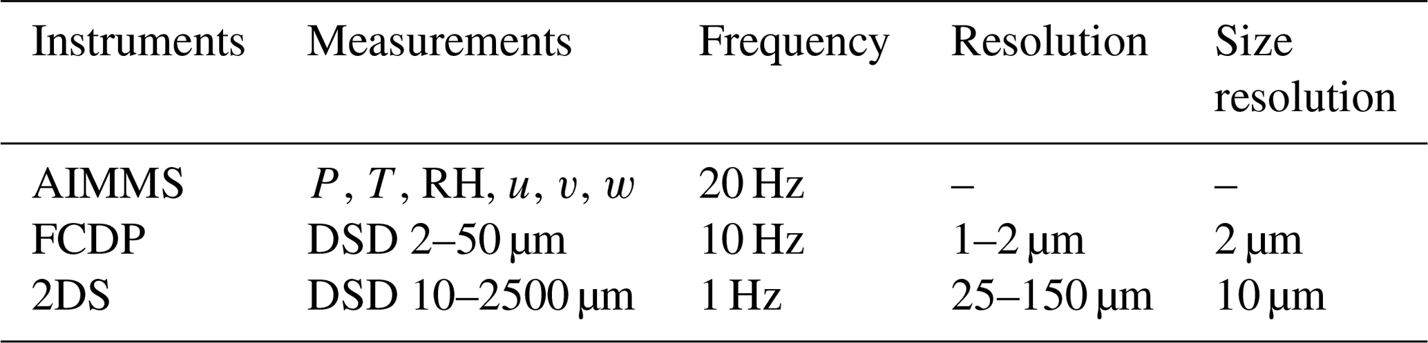
Table 1 summarizes the in situ measurements from the ACE-ENA campaign used in this study. The location and velocity of G-1 aircraft and the environmental and meteorological conditions during the flight (temperature, humidity, and wind velocity) are taken from Aircraft-Integrated Meteorological Measurement System 20 Hz (AIMMS-20) dataset (Beswick et al., 2008). The size distribution of cloud droplets and the corresponding qc and Nc are obtained from the fast cloud droplet probe (FCDP) measurement. The FCDP measures the concentration and size of cloud droplets in the diameter size range from 1.5 to 50 µm in 20 size bins with an overall uncertainty of size around 3 µm (Lance et al., 2010; SPEC, 2019). Following previous studies (Wood, 2005a), we adopt µm as the threshold to separate cloud droplets from drizzle drops; i.e., drops with are considered cloud droplets. After the separation, the qc and Nc are derived from the FCDP droplet size distribution measurements. As an evaluation, we compared our FCDP-derived qc results with the direct measurements of qc from the multi-element water content system (WCM-2000; Matthews and Mei, 2017) also flown during the ACE-ENA and found a reasonable agreement (e.g., biases within 20 %). We also performed a few sensitivity tests in which we perturbed the value of r∗ from 15 up to 50 µm. The perturbation shows little impact on the results shown in Sects. 4 and 5. The cloud droplet spectrum from the FCDP is available at a frequency of 10 Hz, which is used in this study. We have also done a sensitivity study, in which we averaged the FCDP data to 1 Hz and got almost identical results. Since the typical horizontal speed of the G-1 aircraft during the in-cloud leg is about 100 m s−1, the spatial sampling rate these instruments is on the order of 10 m for the FCDP at 10 Hz.
Table 1In situ cloud instruments from ACE-ENA campaign used in this study.
2.2 Ground observations from the ARM ENA site
In addition to the in situ measurements, ground measurements from the ARM ENA site are also used to provide ancillary data for our studies. In particular, we will use the Active Remote Sensing of Cloud Layers product (ARSCL; Clothiaux et al., 2000; Kollias et al., 2005) which blends radar observations from the Ka-band ARM zenith cloud radar (KAZR), the micropulse lidar (MPL), and the ceilometer to provide information on cloud boundaries and the mesoscale structure of cloud and precipitation. The ARSCL product is used to specify the vertical location of the G-1 aircraft and thereby the in situ measurements with respect to the cloud boundaries, i.e., cloud base and top (see example in Fig. 1). In addition, the radar reflectivity observations from KAZR, alone with in situ measurements, are used to select the precipitating cases for our study. Note that the ARSCL product is from the vertically pointing instruments, which sometimes are not collocated with the in situ measurements from G-1 aircraft. As explained later in the next section, only those cases with a reasonable collocation are selected for our study.
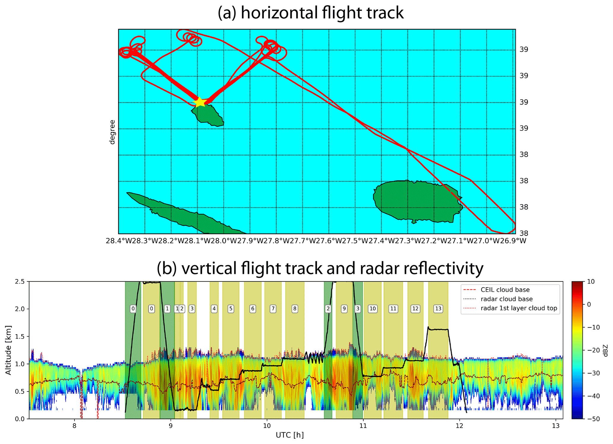
Figure 1(a) Horizontal flight track of the G-1 aircraft (red) during the 18 July 2017 RF around the DOE ENA site (yellow star) on Graciosa Island. (b) The vertical flight track of G-1 (thick black line) overlaid on the radar reflectivity contour by the ground-based KZAR. The dotted lines in the figure indicate the cloud base and top retrievals from ground-based radar and CEIL instruments. The yellow-shaded regions are the “hlegs” and green-shaded regions are the “vlegs”. See text for their definitions.
3.1 ACE-ENA flight pattern
The section provides a brief overview of the G-1 aircraft flight patterns during the ACE-ENA and explains the method for case selections for our study using the 18 July 2017 RF as an example. As shown in Table 2, a variety of MBL conditions were sampled during the two IOPs of the ACE-ENA campaign, from mostly clear sky to thin stratus and drizzling stratocumulus. The basic flight patterns of G-1 aircraft in the ACE-ENA included spirals to obtain vertical profiles of aerosol and clouds, as well as legs at multiple altitudes, including below cloud, inside cloud, at the cloud top, and in the free troposphere. As an example, Fig. 1a shows the horizontal location of the G-1 aircraft during the 18 July 2017 RF, which is the “golden case” for our study as explained in the next section. The corresponding vertical track of the aircraft is shown in Fig. 1b overlaid on the reflectivity curtain of the ground-based KAZR. In this RF, the G-1 aircraft repeated the horizontal level runs multiple times in a V shape at different vertical levels inside, above, and below the MBL (see Fig. 1b). The lower tip of the V shape is located at the ENA site on Graciosa Island. The average wind in the upper MBL (i.e., 900 mbar) is approximately Northwest. So, the west side of the V-shape horizontal level runs is along the wind and the east side across the wind. Note that the horizontal velocity of the G-1 aircraft is approximately 100 m s−1. Since the duration of these selected V-shaped hlegs is between 580 and 700 s, their total horizontal length is roughly 60 km, with each side of the V shape ∼ 30 km. These V-shape horizontal level runs, with one side along and the other across the wind, are a common sampling strategy used in the ACE-ENA to observe the properties of aerosol and cloud at different vertical levels of the MBL. In our study we use the vertical location of the G-1 aircraft from the AIMMS to identify continuous horizontal flight tracks which are referred to as the “hlegs”. For the 18 July 2017 case, a total of 13 hlegs are identified as shown in Fig. 1b. Among them, hlegs 5, 6, 7, 8, 10, 11, and 12 are the seven V-shape horizontal level runs inside the MBL cloud. Together they provide an excellent set of samples of the MBL cloud properties at different vertical levels of a virtual GCM grid box of about 30 km. As previously mentioned, Boutle et al. (2014) found that the horizontal variance of qc increases with the horizontal scale L slowly when L is larger than about 20 km. Therefore, although the horizontal sampling of the selected hlegs is only about 30 km, the lessons learned here could yield useful insights for larger GCM grid sizes. In addition to the hlegs, we also identified the vertical penetration legs in each flight, referred to as the “vlegs”, from which we will obtain the vertical structure of the MBL, along with the properties of cloud and aerosol.
Table 2Conditions of MBL sampled during the two IOPs of the ACE-ENA campaign. Dates are given in month and day (m/dd) format.

3.2 Case selection
As illustrated in Fig. 1a and b for the 18 July 2017 RF, the criteria we used to select the RF cases and the hlegs within the RF can be summarized as follows:
-
The RF samples multiple continuous in-cloud hlegs at different vertical levels with the horizontal length of at least 10 km and cloud fraction larger than 10 % (i.e., the fraction of an hleg with qc > 0.01 g m−3 must exceed 10 % of the total length of that hleg). It is important to note here that, unless otherwise specified, all the analyses of qc and Nc are based on in-cloud observations (i.e., in the regions with qc > 0.01 g m−3).
-
Moreover, the selected hlegs must sample the same region (i.e., the same virtual GCM grid box) repeatedly in terms of horizontal track but different vertical levels in terms of vertical track. Take the 18 July 2017 case as an example. The hlegs 5, 6, 7, and 8 follow the same V-shaped horizontal track (see Fig. 1a) but sample different vertical levels of the MBL clouds (see Fig. 1b). Such hlegs provide us the horizontal sampling needed to study the subgrid horizontal variations of the cloud properties and, at the same time, the chance to study the vertical dependence of the horizontal cloud variations.
-
Finally, the RF needs to have at least one vleg, and the cloud boundary derived from the vleg is largely consistent with that derived from the ground-based measurements. This requirement is to ensure that the vertical locations of the selected hlegs with respect to cloud boundaries can be specified. For example, as shown in Fig. 1b according to the ground-based observations, hlegs 5 and 10 of the 18 July 2017 case are close to cloud base, while hlegs 8 and 12 are close to cloud top (see also Fig. 4).
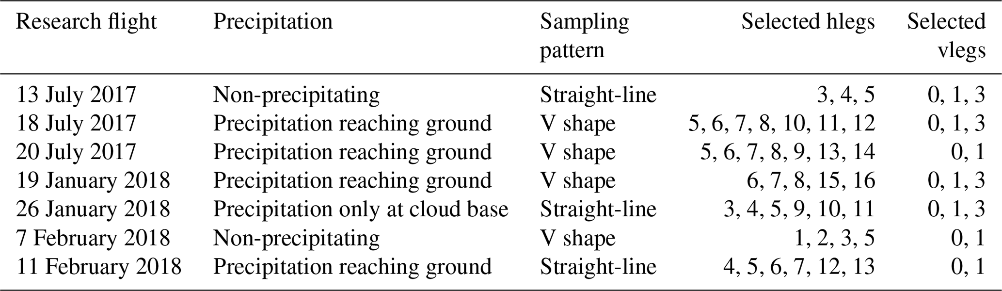
The above requirements together pose a strong constraint on the observation. Fortunately, thanks to the careful planning of the RF, which had already taken studies like ours into consideration, we are able to select a total of seven RF cases as summarized in Table 3. The plots of the flight tracks and ground-based radar observations for the six other RF cases are provided in the Supplement (Figs. S1–S6). We will first focus on the golden case – 18 July 2017 RF – and then investigate if the lessons learned from the 18 July 2017 RF also apply to the other three cases.
Table 3A summary of selected RFs and the selected hlegs and vlegs within each RF.
4.1 Horizontal and vertical variations of cloud microphysics
On 18 July 2017, the North Atlantic is controlled by the Icelandic low to the north and the Azores high to the south (see Fig. 2b), which is a common pattern of large-scale circulation during the summer season in this region (Wood et al., 2015). The Azores is at the southern tip of the cold air sector of a frontal system where the fair-weather low-level stratocumulus clouds are dominant (see satellite image in Fig. 2a). The RF on this day started around 08:30 UTC and ended around 12:00 UTC. As explained in the previous section, we selected seven hlegs from this RF that horizontally sampled the same region repeatedly in a similar V-shaped track but vertically at different levels. The radar reflectivity observation from the ground-based KAZR during the same period peaks around 10 dBZ, indicating the presence of significant drizzle inside the MBL clouds.
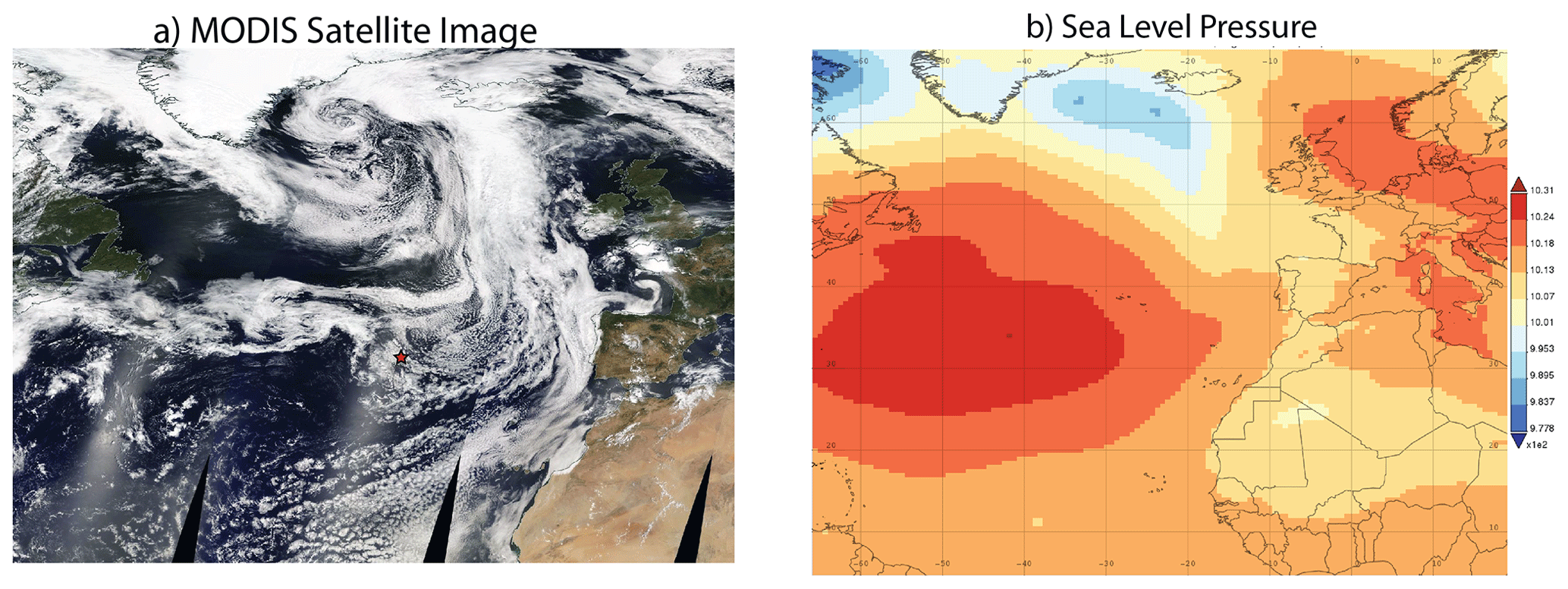
Figure 2(a) The real color satellite image of the ENA region on 18 July 2017 from MODIS. The small red star marks the location of the ARM ENA site on Graciosa Island. (b) The averaged sea level pressure (SLP) of the ENA region on 18 July 2017 from the MERRA-2 reanalysis.
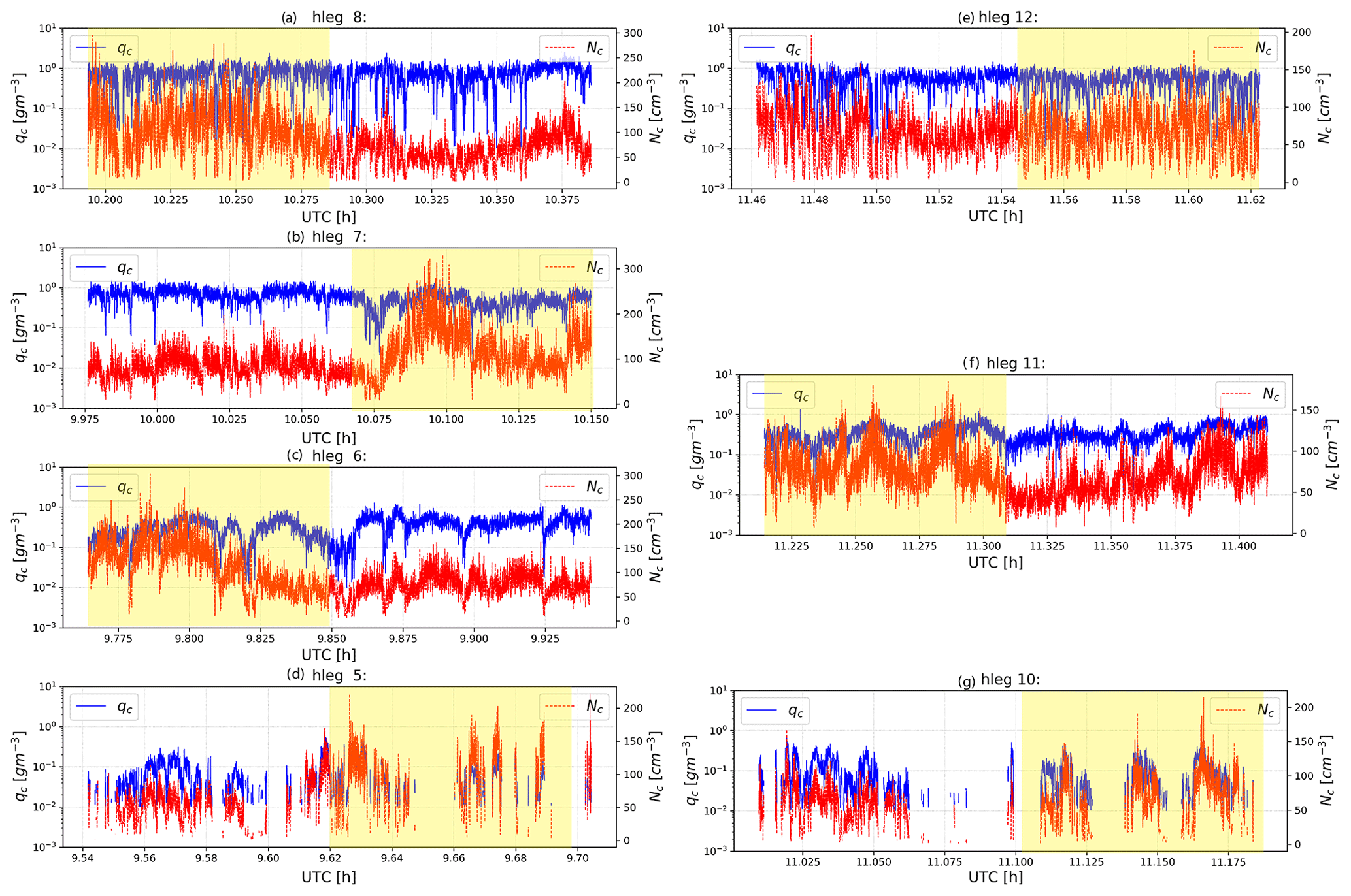
Figure 3The horizontal variations of qc (red) and Nc (blue) for each selected hleg derived from the in situ FCDP instrument. The yellow-shaded time period in each plot corresponds to the cross-wind side of the V-shaped flight track, and the unshaded part corresponds to the along-wind part. Note that plots are ordered such that (a) hleg 8 and (e) hleg 12 are close to cloud top; (b) hleg 6, (c) hleg 7, and (f) hleg 11 are sampled in the middle of clouds; and (d) hleg 5 and (g) hleg 10 are close to cloud base.
Among the seven selected hlegs, hlegs 5, 6, 7, and 8 constitute one set of four consecutive V-shaped tracks, with hlegs 5 close to cloud base and hleg 8 close to cloud top. The hlegs 10, 11, and 12 are another set of consecutive V-shaped tracks with hlegs 10 and 12 close to cloud base and top, respectively (see Fig. 1). Using qc>0.01 g m−3 as a threshold for cloud, the cloud fraction (fc) of all these hlegs is close to unity (i.e., overcast), except for the two hlegs close to cloud base (fc= 46 % for hleg 5 and fc= 51 % for hleg 10). The qc and Nc derived from the in situ FCDP measurements for these selected hlegs are plotted in Fig. 3 as a function of UTC time. It is evident from Fig. 3 that both qc and Nc have significant horizontal variations. At cloud base (see Fig. 3d for hleg 5 and Fig. 3g for hleg 10) the qc varies from 0.01 g m−3 (i.e., the lower threshold) up to about 0.4 g m−3 and the Nc from 25 up to 150 cm−3, with the mean in-cloud values around 0.08 g m−3 and 65 cm−3, respectively. Such strong variations of cloud microphysics could be contributed by a number of factors. One can see from the ground radar and lidar observations in Fig. 1b that the height of cloud base varies significantly. As a result, the horizonal legs may not really sample the cloud base. In addition, the variability in updraft at cloud base could lead to the variability in the activation and growth of cloud condensation nuclei (CCN). In the middle of the MBL cloud, i.e., hleg 6 (Fig. 3c), 7 (Fig. 3b) and 11 (Fig. 3f), the mean value of qc is significantly larger than that of cloud base hlegs while the variability is reduced. The mean value of qc keeps increasing toward cloud top to ∼ 0.73 g m−3 in hleg 8 (Fig. 3a) and to ∼ 0.53 g m−3 in hleg 12 (Fig. 3e), respectively. In contrast, the horizontal variability of qc seems to increase in comparison to those observed in mid-level hlegs.
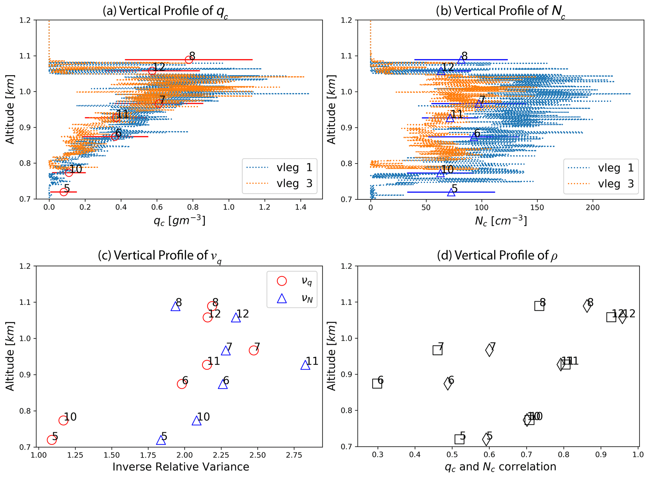
Figure 4(a) The vertical profiles of qc derived from the vlegs (dotted lines) of the 18 July 2017 case. The overplotted red error bars indicate the mean values and standard deviations of the qc derived from the selected hlegs at different vertical levels. (b) Same as panel (a) except for Nc. (c) The vertical profile of the inverse relative variances (i.e., mean divided by standard deviation) of Nc (red circle) and Nc (blue triangle) derived from the hleg; (d) the vertical profile of the linear correlation coefficient between ln (qc) and ln (Nc), i.e., ρL (square), and the linear correlation coefficient between qc and Nc, i.e., ρ (diamond).
To obtain a further understanding of the vertical variations of cloud microphysics, we analyzed the cloud microphysics observations from the two green-shaded vlegs 1 and 3 in Fig. 1b. The vertical profiles of the mean qc and Nc from these two vlegs are shown in Fig. 4a and b, respectively, with the mean and standard deviation of the qc and Nc derived from the seven selected hlegs overplotted. Overall, the vertical profiles of the qc and Nc are qualitatively aligned with the classic adiabatic MBL cloud structure (Brenguier et al., 2000; Martin et al., 1994). That is, the Nc remains relatively constant (see Fig. 4b), while the qc increases approximately linearly with height from cloud base upward as a result of condensation growth (see Fig. 4a,), except for the very top of the cloud, i.e., the entrainment zone where the dry air entrained from above mixes with the humid cloudy air in the MBL. In previous studies, a so-called inverse relative variance, ν, is often used to quantify the subgrid variations of cloud microphysics. It is defined as follows:
where X is either qc (i.e., ) or Nc (i.e., ) (Barker et al., 1996; Lebsock et al., 2013; Zhang et al., 2019). 〈x〉 and σX are the mean value and standard deviation of X, respectively. As such, the smaller the ν value, the larger the horizontal variation of X in comparison to the mean value. As shown in Fig. 4c, the and derived from the selected hlegs follow a similar vertical pattern: they both increase first from cloud base upward and then decrease in the entrainment zone, with the turning point somewhere around 1 km (i.e., around hleg 7 and 11). It indicates that both qc and Nc have significant horizontal variabilities at cloud base which may be a combined result of horizontal fluctuations of dynamics (e.g., updraft) and thermodynamics (e.g., temperature and dynamics), as well as horizontal variations of aerosols. The horizontal variabilities of both qc and Nc both decrease upward toward cloud top until the entrainment zone where both variabilities increase again.
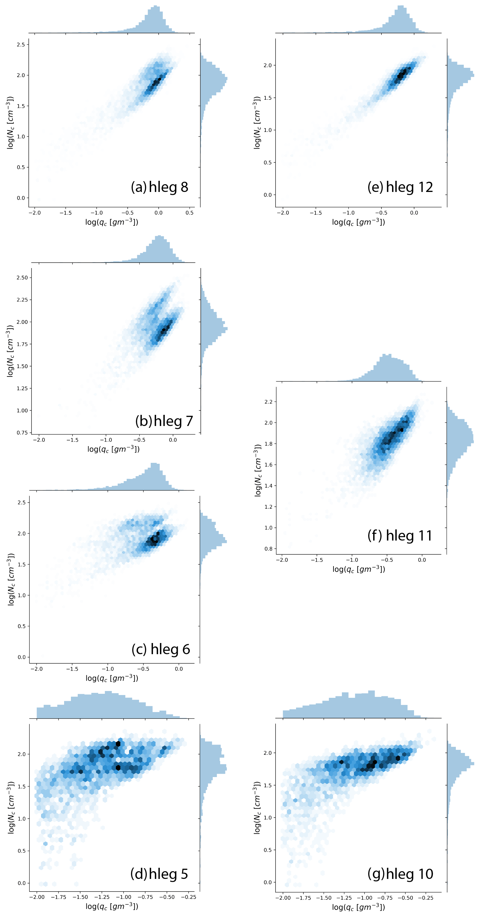
Figure 5The joint distributions of qc and Nc, along with the marginal histograms, for the seven selected hlegs from the 18 July 2017 RF. As in Fig. 3, the plots are ordered such that (a) hleg 8 and (e) hleg 12 are close to cloud top; (b) hleg 6, (c) hleg 7, and (f) hleg 11 are sampled in the middle of clouds; and (d) hleg 5 and (g) hleg 10 are close to cloud base.
So far, in all the analyses above, the variations of qc and Nc have been considered separately and independently. As pointed out in several previous studies, the covariation of qc and Nc could have an important impact on the EF for the autoconversion process in GCMs (Kogan and Mechem, 2016; Larson and Griffin, 2013; Zhang et al., 2019). This point will be further elucidated in detail in the next section. Figure 5 shows the joint distributions of qc and Nc for the seven selected hlegs, and the corresponding linear correlation coefficients as a function of height are shown in Fig. 4d. For the sake of reference, the linear correlation coefficient between ln (qc) and ln (Nc) , i.e., the ρL that will be introduced later in Eq. (4), is also plotted in Fig. 4d. Looking first at hlegs 10, 11, and 12, i.e., the second group of consecutive V-shaped legs, there is a clear increasing trend of the correlation between qc and Nc from cloud bottom (ρ=0.75 for hleg 10) to cloud top (ρ=0.95 for hleg 12). The picture based on hlegs 5, 6, 7, and 8 is more complex. As shown in Fig. 5, the joint distributions of qc and Nc of hleg 6 (Fig. 5b), hleg 7 (Fig. 5c), and, to a less extent, hleg 8 (Fig. 5d) all exhibit a clear bimodality. Further analysis reveals that each of the two modes in these bimodal distributions approximately corresponds to one side of the V-shaped track. To illustrate this, the east side (i.e., across wind) of the hleg is shaded in yellow in Fig. 3. It is intriguing to note that the Nc values from the east side of the hleg are systematically larger than those from the west side, while their qc values are largely similar. It is unlikely that the bimodality is caused by the along-wind and across-wind difference between the two sides of the V-shaped track. It is most likely just a coincidence. On the other hand, the bimodal joint distribution between qc and Nc is real, which could be a result of subgrid variations of updraft, precipitation, and/or aerosols.
As a result of the bimodality of Nc, the correlation coefficients between qc and Nc is significantly smaller for hlegs 6 (ρ=0.22) and 7 (ρ=0.31) in comparison to other hlegs. However, if the two sides of the V-shaped tracks are considered separately, then qc and Nc become more correlated, except for the east side of hleg 6, which still exhibits to some degree a bimodal joint distribution of qc and Nc. In spite of the bimodality, there is evidently a general increasing trend of the correlation between qc and Nc from cloud base toward cloud top. At the cloud top, the qc and Nc correlation coefficient can be as high as ρ=0.95 for hleg 12 (see Fig. 5e). As explained in the next section, this close correlation between qc and Nc has important implications for the simulation of the autoconversion enhancement factor.
As a summary, the above phenomenological analysis of the 18 July 2017 RF reveals the following features of the horizontal and vertical variations of cloud microphysics. Vertically, the mean values of qc and Nc qualitatively follow the adiabatic structure of MBL cloud; i.e., qc increases linearly with height and Nc remains largely invariant above cloud base. Even though the joint distribution of qc and Nc exhibits a bimodality in several hlegs, their correlation generally increases with height and can be as high as ρ=0.95 at cloud top. Horizontally, both qc and Nc have a significant variability at cloud base, which tends to first decrease upward and then increase in the uppermost part of cloud close to the entrainment zone. Finally, we have to point out a couple of important caveats in the above analysis. First, as seen from Fig. 1 the selected hlegs are sampled at different vertical locations and also at different times. For example, hleg 5 at cloud base is more than 1 h apart from hleg 8 at cloud top (Fig. 1a). As a result, the temporal evolution of clouds is a confounding factor and might be misinterpreted as vertical variations of clouds. On the other hand, as shown below, we also observed similar vertical structure of qc and Nc in other cases. It seems highly unlikely that the temporal evaluations of the clouds in all selected cases conspire to confound our results in the same way. Based on this consideration, we assume that the temporal evolution of clouds is an uncertainty that could lead to random errors but does not impact the overall vertical trend. The second caveat is that due to the very limited vertical sampling rate of hlegs (i.e., only 3–4 samples), we cannot possibly resolve the detailed vertical variation of νq, νN, and ρ. Although we have used the word “trend” in the above analysis, it should be noted that the vertical profile of these parameters may, but more likely may not, be linear. So, the word “trend” here indicates only the large pattern that can be resolved by the hlegs. Obviously these two caveats also apply to the analysis below the EF, which is also derived from the hlegs.
4.2 Implications for the EF for the autoconversion rate parameterization
As explained in the introduction, in GCMs the autoconversion process is usually parameterized as a highly nonlinear function of qc and Nc, e.g., the KK scheme in Eq. (1). In such a parameterization, an EF is needed to account for the bias caused by the nonlinearity effect. A variety of methods have been proposed and used in the previous studies to estimate the EF (Larson and Griffin, 2013; Lebsock et al., 2013; Pincus and Klein, 2000; Zhang et al., 2019). The methods used in this study are based on Z19. Only the most relevant aspects are recapped here. Readers are referred to Z19 for detail.
If the subgrid variations of qc and Nc, as well as their covariation, are known, then the EF can be estimated based on its definition as follows:
where 〈qc〉 and 〈Nc〉 are the grid-mean value, P(qc,Nc) is the joint probability density function (PDF) of qc and Nc. qc,min and Nc,min are the lower limits of the in-cloud value (e.g., g m−3). Some previous studies approximate the P(qc,Nc) as a bivariate lognormal distribution as follows:
where μX and σX are, respectively, the mean and standard deviation of ln (X), where X is either qc or Nc. ρL is the linear correlation coefficient between ln (qc) and ln (Nc) (Larson and Griffin, 2013; Lebsock et al., 2013; Zhang et al., 2019). It should be noted here that ρL is fundamentally different from ρ (i.e., the linear correlation coefficient between qc and Nc). On the other hand, we found that for all the selected hlegs, ρ and ρL are in an excellent agreement (see Fig. 4d). In fact, ρ and ρL can be used interchangeably in the context of this study without any impact on the conclusions. Nevertheless, interested readers may find more detailed discussion of the relationship between ρ and ρL in Larson and Griffin (2013).
Substituting P(qc,Nc) in Eq. (4) into Eq. (3) yields a formula for EF that consists of the following three terms:
where corresponds to the enhancing effect of the subgrid variation of qc, if qc follows a marginal lognormal distribution, i.e., . It is a function of the inverse relative variance νq in Eq. (2) as follows:
Similarly, the below corresponds to the enhancing effect of the subgrid variation of Nc, if Nc follows a marginal lognormal distribution:
The third term in Eq. (5),
corresponds to the impact of the covariation of qc and Nc on the EF. Because βq>0 and βN<0, if qc and Nc are negatively correlated (i.e., ρL<0), then the ECOV>1 and acts as an enhancing effect on the autoconversion rate computation. In contrast, if qc and Nc are positively correlated (i.e., ρL>0), then the ECOV<1, which becomes a suppressing effect on the autoconversion rate computation.
As previously mentioned, most previous studies of the EF consider only the impact of subgrid qc variation (i.e., only the Eq term). The impacts of subgrid Nc variation as well as its covariation with qc have been largely overlooked in observational studies, in which the Eq is often derived from the observed subgrid variation of qc based on the definition of EF, i.e.,
where P(qc) is the observed subgrid PDF of qc. Alternatively, Eq has also been estimated from the inverse relative variance νq by assuming the subgrid variation of qc follows the lognormal distribution, in which case Eq is given in Eq. (6).
Similar to EN, if only the effect of subgrid Nc is considered, the corresponding EN can be derived from the following two ways: one from the observed subgrid PDF P(Nc) based on the definition of EF, i.e.,
and the other based on Eq. (7) from the relative variance by assuming the subgrid Nc variation follows the lognormal distribution.
Now, we put the in situ qc and Nc observations from the selected hlegs in the theoretical framework of EF described above and investigate the following questions:
-
What is the (observation-based) EF derived based on Eq. (3) from the observed joint PDF P(qc,Nc)?
-
How well does the (bi-logarithmic) EF derived based on Eq. (5) by assuming that the covariation of qc and Nc follows a bivariate lognormal agree with the observation-based EF?
-
What is the relative importance of the Eq, EN, and ECOV terms in Eq. (5) in determining the value of EF?
-
What is the error of considering only Eq and omitting the EN and ECOV terms?
-
How do the observation-based EFs from Eq. (3) and the Eq, EN, and ECOV terms vary with vertical height in cloud?
These questions are addressed in the rest of this section. Focusing first on the Eq in Fig. 6a, the Eq derived from observation based on Eq. (9) (solid circle) shows a clear decreasing trend with height between cloud base at around 700 m to about 1 km, with a value reduced from about 3 to about 1.2. Then, the value of Eq increases slightly in the cloud top hlegs 8 and 12. The Eq derived based on Eq. (6) by assuming lognormal distribution (open circle) has a very similar vertical pattern, although the value is slightly overestimated on average by 0.07 in comparison to the observation-based result. The vertical pattern of Eq can be readily explained by the subgrid variation of qc in Fig. 4c. The EN derived from observation (solid triangle) in Fig. 6b shows a similar vertical pattern as Eq, i.e., first decreasing with height from cloud base to about 1.2 km and then increasing with height in the uppermost part of cloud. The EN derived based on Eq. (7) by assuming a lognormal distribution (open triangle) significantly underestimates the observation-based values (mean bias of −4.3), especially at cloud base (i.e., hleg 5 and 10) and cloud top (i.e., hleg 8 and 12).
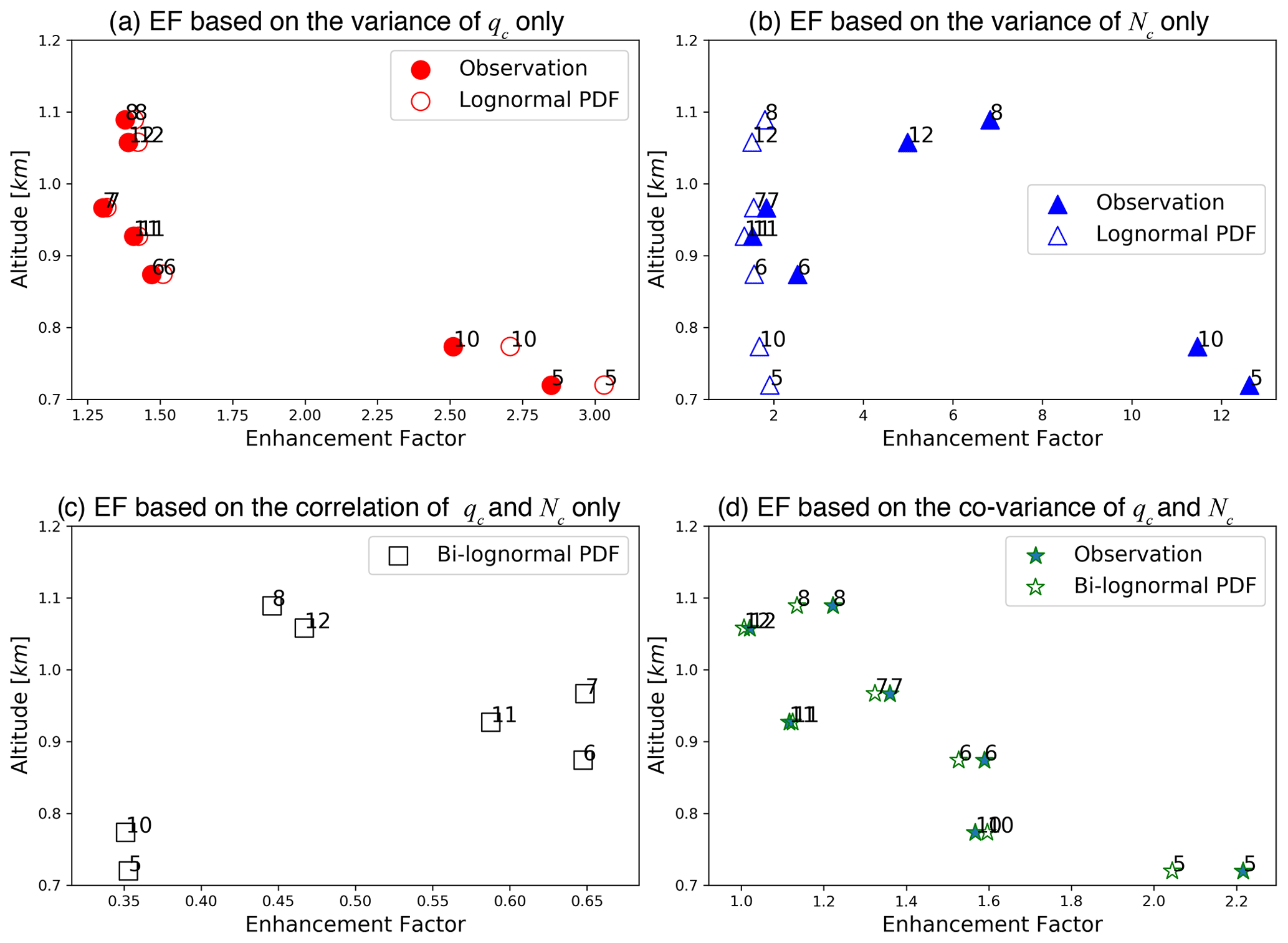
Figure 6(a) Eq as a function of height derived from observation based on Eq. (9) (solid circle) and from the inverse relative variance νq assuming lognormal distribution based on Eq. (6) (open circle). (b) EN as a function of height derived from observation based on Eq. (10) (solid triangle) and from the inverse relative variance νN assuming lognormal distribution based on Eq. (7) (open triangle). (c) ECOV derived based on Eq. (8) as a function of height. (d) E as a function of height derived from observation based on Eq. (3) (solid star) and based on Eq. (5) assuming a bi-lognormal distribution (open star). The numbers beside the symbols in the figure correspond to the numbers of the seven selected hlegs.
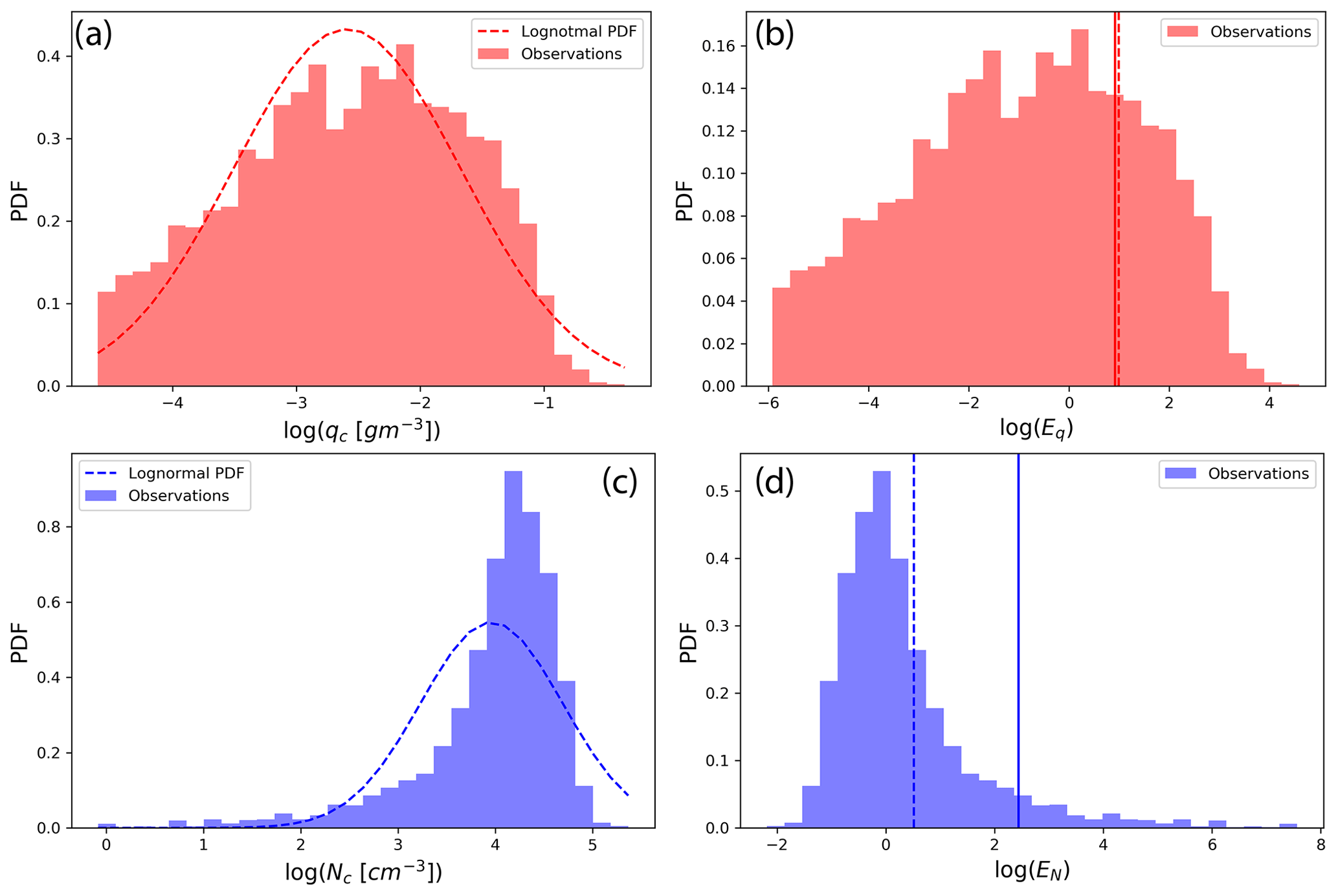
Figure 7(a) Histogram of ln (qc) based on observations from hleg 10 (bars) and the lognormal PDF (dashed line) based on the and of hleg 10. (b) The histogram of ln (Eq) diagnosed from the observed qc based on Eq. (9). The two vertical lines correspond to the leg-averaged ln (Eq) derived based on the observed qc (solid) and the lognormal PDF (dashed line), respectively. (c) Histogram of ln (Nc) based on observations from hleg 10 (bars) and the lognormal PDF (dashed line) based on the and of hleg 10. (d) The histogram of ln (EN) diagnosed from the observed qc based on Eq. (10). The two vertical lines correspond to the leg-averaged ln (EN) derived based on the observed Nc (solid) and the lognormal PDF (dashed line), respectively.
Using hleg 10 as an example, we further investigated the cause for the error in lognormal-based EFs in comparison to those diagnosed from the observation. As shown in Fig. 7a the observed qc is slightly negatively skewed in logarithmic space by the small values. Because the autoconversion rate is proportional to , the negatively skewed qc also leads to a negatively skewed Eq in Fig. 7b. As a result, the leg-averaged Eq diagnosed from the observation is slightly smaller than that derived based on Eq. (6) by assuming a lognormal distribution. The negative skewness also explains the large error in EN for hleg 10 seen on Fig. 6b. As shown in Fig. 7c the observed Nc is also negatively skewed to a much larger extent in comparison to qc. Because the autoconversion rate is proportional to , the highly negatively skewed Nc results in a highly positively skewed EN in Fig. 7d. As a result, the EN diagnosed from the observation is much larger than that derived based on Eq. (7) by assuming a lognormal distribution.
The Eq and EN reflect only the individual contributions of subgrid qc and Nc variations to the EF. The effect of the covariation of qc and Nc, i.e., the ECOV, is shown in Fig. 6c. Interestingly, the value of ECOV is smaller than unity for all the selected hlegs. As explained in Eq. (8), ECOV<1 is a result of a positive correlation between qc and Nc, as seen in Fig. 4d. Therefore, in these hlegs the covariation of the qc and Nc has a suppressing effect on the EF, in contrast to the enhancing effect of Eq and EN. This result is qualitatively consistent with Z19, who found that the vertically integrated liquid water path (LWP) of MBL clouds is in general positively correlated with the Nc estimated from the MODIS cloud retrieval product and, as a result, ECOV<1 over most of the tropical oceans. Because of the relationship in Eq. (8), the value ECOV is evidently negatively proportional to the correlation coefficient ρL in Fig. 4d. The largest value is seen in hleg 6 and 7, in which the bimodal joint distribution of qc and Nc results in a small ρL. A rather small value of ECOV∼0.45 is seen for cloud top hleg 8 and 12, as result of a strong correlation between qc and Nc (ρL>0.9) and moderate σq and σN.
Finally, the EF that accounts for all factors, including the individual variations of qc and Nc, as well as their covariation, is shown in Fig. 6d. Focusing first on the observation-based results (solid star), i.e., E in Eq. (3), evidently there is a decreasing trend from cloud base (e.g., E=2.2 for hleg 5 and E=1.59 for hleg 10) to cloud top (e.g., E=1.20 for hleg 8 and E=1.02 for hleg 12). The E values derived based on Eq. (5) by assuming the bivariate lognormal distribution between qc and Nc (i.e., open star in Fig. 6d) are in reasonable agreement with the observation-based results, with a mean bias of −0.09. It is intriguing to note that the value of in Fig. 6d is comparable to Eq in Fig. 6a, which indicates that the enhancing effect of EN>1 in Fig. 6b is partially canceled by the suppressing effect of ECOV<1 in Fig. 6c. As previously mentioned, many previous studies of the EF consider only the effect of Eq but overlook the effect of EN and ECOV. The error in the studies would be quite large if it were not for a fortunate error cancellation.
In addition to the 18 July 2017 RF, we also found another six RFs that meet our criteria as described in Sect. 3 for case selection, from non-precipitating (e.g., 13 July 2017 case in Fig. S1) to weakly (e.g., 26 January 2018 case in Fig. S4) and heavily precipitating cloud (11 February 2018 case in Fig. S6). Due to limited space, we cannot present the detailed case studies of these RFs. Instead, we view them collectively and investigate whether the lessons learned from the 18 July 2017 RF, especially those about the EF in Sect. 4.2, also apply to the other cases.
In order to compare the hlegs from different RFs, we first normalize the altitude of each hleg with respect to the minimum and maximum values of all selected hlegs in each RF as follows:
where is the normalized altitude for each hleg in a RF, and zmin and zmax are the altitude of the lowest and highest hleg in the corresponding RF. Defined this way, is bounded between 0 and 1. Alternatively, could also be defined with respect to the averaged cloud top (ztop) and base (zbase) as inferred from the KAZR or vlegs. However, because of the variation of cloud top and cloud base heights, as well as the collocation error, the would often become significantly larger than 1 or smaller than 0, if were defined with respect to ztop and zbase, making results confusing and difficult to interpret.
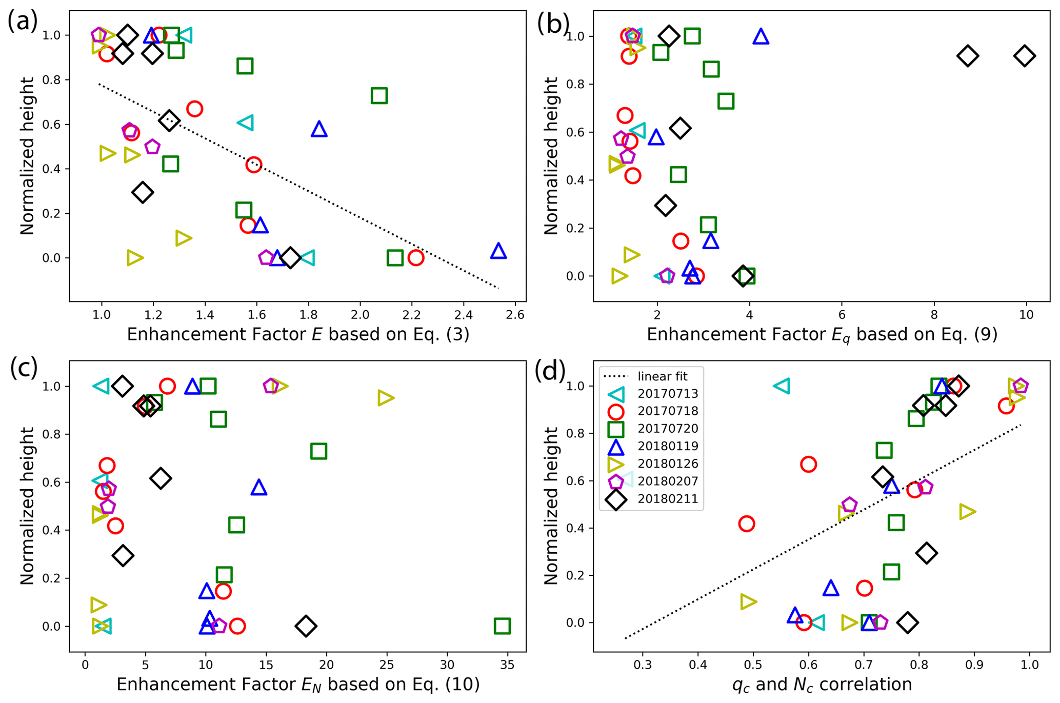
Figure 8(a) The observation-based E derived from Eq. (3) that accounts for the covariation of qc and Nc. (b) The observation-based Eq derived from Eq. (9) that accounts for only the subgrid variation of qc. (c) The observation-based EN derived from Eq. (10) that accounts for only the subgrid variation of Nc. (d) The correlation coefficient between qc and Nc. All quantities are plotted as a function of the normalized height in Eq. (11). The dashed lines correspond to a linear fit of the data when the fitting is statistically significant (i.e., P value < 0.05).
Figure 8 shows the observation-based EFs for all the selected hlegs from the seven selected RFs as a function of the . As shown in Fig. 8a, the E derived based on Eq. (3) that accounts for the covariation of qc and Nc has a decreasing trend from cloud base to cloud top. This is consistent with the result from the 18 July 2017 case in Fig. 6d. However, neither the Eq in Fig. 8b nor the EN in Fig. 8c shows a clear dependence on in comparison to the results of the 18 July 2017 case in Fig. 6a and b. Note that the Eq and EN are influenced by a number of factors, such as horizontal distance and cloud fraction, in addition to vertical height. It is possible that the differences in other factors outweigh the vertical dependence here. Interestingly, the linear correlation coefficient ρ between qc and Nc in Fig. 8d shows an increasing trend with that is statistically significant (R value =0.50 and P value = 0.02), despite a few outliers. This is consistent with what we found in the 18 July 2017 case (see Fig. 4d). As evident from Eq. (8), an increase in ρL would lead to a decrease in ECOV. Since neither Eq nor EN shows a clear dependence on , the decrease in ECOV with seems to play an important role in the determining the value of E. Another line of evidence supporting this role is the fact that both Eq and EN are quite large for the cloud top hlegs, while in contrast the values of the corresponding E that accounts for the covariation of qc and Nc are much smaller. For example, the Eq for two hlegs from the 11 February 2018 RF exceeds 8, but the corresponding E values are smaller than 1.2, which is evidently a result of large ρL and thereby small ECOV.
As previously mentioned, many previous studies of the EF for the autoconversion rate parameterization consider only the effect of subgrid qc variation but ignore the effects of subgrid Nc variation and its covariation with qc. To understand the potential error, we compared the Eq and E both derived based on observations in Fig. 9. Apparently, Eq is significantly larger than E for most of the selected hlegs, which implies that considering only subgrid qc variation would likely lead to an overestimation of EF. This is an interesting result. Note that EN≥1 by definition and therefore Eq>E is possible only when the covariation of qc and Nc has a suppressing effect, instead of enhancing. Once again, this result demonstrates the importance of understanding the covariation of qc and Nc for understanding the EF for autoconversion rate parameterization.

Figure 9A comparison of observation-based E and observation-based Eq for all the selected hlegs from all four selected RFs.
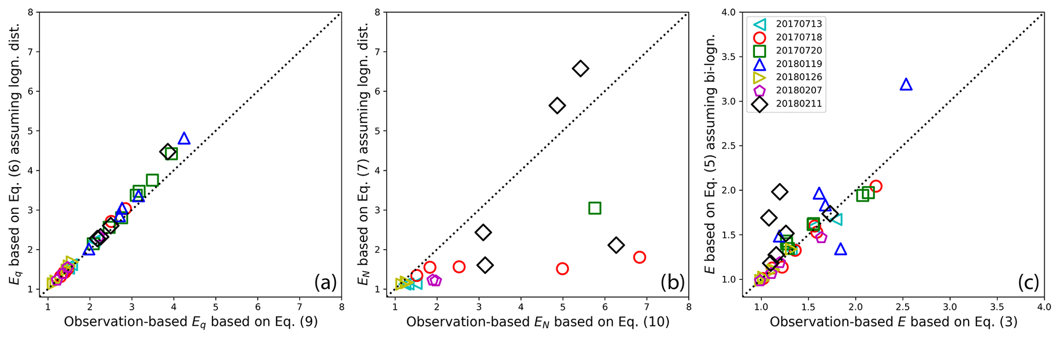
Figure 10(a) A comparison of observation-based Eq derived based on Eq. (9) and Eq derived based on Eq. (6) assuming lognormal distribution for subgrid qc observations for all the selected hlegs. (b) A comparison of observation-based EN derived based on Eq. (10) and EN derived based on Eq. (7) assuming lognormal distribution or all the selected hlegs. (c) A comparison of observation-based E derived based on Eq. (3) and E derived based on Eq. (5) assuming bivariate lognormal distribution for the subgrid joint distribution of qc and Nc.
Having looked at the observation-based EFs, we now check if the EFs derived based on assumed PDFs (e.g., lognormal or bivariate lognormal distributions) agree with the observation-based results. As shown in Fig. 10a, the Eq based on Eq. (6) that assumes a lognormal distribution for the subgrid variation of qc is in an excellent agreement with the observation-based results. In contrast, the comparison is much worse for the EN in Fig. 10b, which is not surprising given the results from the 18 July 2017 case in Fig. 6b. As one can see from Fig. 5, the marginal PDF of Nc is often broad and sometimes even bimodal. The deviation of the observed Nc PDF from the lognormal distribution is probably the reason for the large difference of EN in Fig. 10b. As shown in Fig. 10c, the E values derived based on Eq. (5) by assuming a bivariate lognormal function for the joint distribution of qc and Nc are in good agreement with observation-based values, which is consistent with the results from the 18 July 2017 case in Fig. 6.
In this study we derived the horizontal variations of qc and Nc, as well as their covariations in MBL clouds based on the in situ measurements from the recent ACE-ENA campaign, and investigated the implications of subgrid variability as it relates to the enhancement of autoconversion rates. The main findings can be summarized as follows:
-
In the 18 July 2017 case, the vertical variation of the mean values of qc and Nc roughly follows the adiabatic structure. The horizontal variances of qc and Nc first decrease from cloud base upward toward the middle of the cloud and then increase near cloud top. The correlation between of qc and Nc generally increases from cloud base to cloud top.
-
In other selected cases, the horizontal variances of qc and Nc show no statistically significant dependence on the vertical height in cloud. However, the increasing trend of the correlation between qc and Nc from cloud base to cloud top remains robust.
-
In a few selected V-shaped hlegs, the qc and Nc follow a bimodal joint distribution which leads to a weak linear correlation between them.
-
The observation-based physically complete E that accounts for the covariation of qc and Nc has a robust decreasing trend from cloud base to cloud top, which can be explained by the increasing trend of the qc and Nc correlation from cloud base to cloud top.
-
The E estimated by assuming a monomodal bivariate lognormal joint distribution between qc and Nc agrees well with the observation-based results.
These results provide the following two new understandings of the EF for the autoconversion parameterization that have potentially important implications for GCM. First, our study indicates that the physically complete E has a robust decreasing trend from cloud base to cloud top. Because the autoconversion process is most important at the cloud top, this vertical dependence of EF should be taken into consideration in the GCM parametrization scheme. Second, our study indicates that effect of the qc and Nc correlation plays a critical role in determining the EF. Lately a few novel modeling techniques have been developed to provide the coarse-resolution GCM information of subgrid cloud variation, such as the PDF-based higher-order turbulence closure method – Cloud Layer Unified By Binormals (CLUBB; Golaz et al., 2002; Guo et al., 2015; Larson et al., 2002). These models are able to provide the parameterized subgrid variance of qc, which can be used in turn to estimate Eq. However, as shown in our study the Eq tends to overestimate the EF.
Our study has a few important limitations. First of all, our results are based on a handful cases from a single field campaign. The lessons learned here need to be further examined based on more data or tested in modeling studies. Second, as pointed out in Sect. 4.1, due to the inherent sampling limitation of airborne measurements, the temporal evolution of clouds is an important uncertainty and a confounding factor in this study, which needs to be quantified in future studies. Third, our study provides only a phenomenological analysis of the horizontal variations of cloud microphysics in the MBL clouds and the implications for the EF. Ongoing modeling research based on a comprehensive LES model is being conducted to identify and elucidate the process-level physical mechanisms behind our observational results. Finally, this study is focused on the KK parameterization in estimating the enhancement factors resulting from subgrid variability of qc, Nc, and qc–Nc covariance. The specific values are expected to differ when applied to other autoconversion parameterizations with different power-law exponents.
All the Python codes used in this study are in Jupyter notebook format and can be made available from the corresponding author upon request.
The in situ measurements from the DOE ACE-ENA campaign are available from the DOE data center at https://adc.arm.gov/discovery/#/results/s::ACE-ENA (Atmospheric Radiation Measurement, 2021).
The supplement related to this article is available online at: https://doi.org/10.5194/acp-21-3103-2021-supplement.
ZZ collected the in situ measurements, performed the analysis, and drafted the manuscript. QS helped with the data analysis and figures. DBM, VEL, JW, YL, MKW, XD, and PW provided comments on the manuscript and helped with the revision.
The authors declare that they have no conflict of interest.
This article is part of the special issue “Marine aerosols, trace gases, and clouds over the North Atlantic (ACP/AMT inter-journal SI)”. It is not associated with a conference.
Zhibo Zhang acknowledges the financial support from the Atmospheric System Research (grant no. DE-SC0020057) funded by the Office of Biological and Environmental Research in the US DOE Office of Science. The computations in this study were performed at the UMBC High Performance Computing Facility (HPCF). The facility is supported by the US National Science Foundation through the MRI program (grant nos. CNS-0821258 and CNS-1228778) and the SCREMS program (grant no. DMS-0821311), with substantial support from UMBC. David B. Mechem was supported by subcontract OFED0010-01 from the University of Maryland Baltimore County and the US Department of Energy's Atmospheric Systems Research grant DE-SC0016522.
This research has been supported by the US Department of Energy Office of Science (grant nos. DE-SC0020057 and DE-SC0016522) and the National Science Foundation (grant nos. CNS-0821258, CNS-1228778, and DMS-0821311).
This paper was edited by Armin Sorooshian and reviewed by three anonymous referees.
Ahlgrimm, M. and Forbes, R. M.: Regime dependence of cloud condensate variability observed at the Atmospheric Radiation Measurement Sites, Q. J. R. Meteor. Soc., 142, 1605–1617, https://doi.org/10.1002/qj.2783, 2016.
Atmospheric Radiation Measurement: ACE-ENA field campaign data, available at: https://adc.arm.gov/discovery/#/results/s::ACE-ENA, last access: 28 February 2021.
Barker, H. W., Wiellicki, B. A., and Parker, L.: A Parameterization for Computing Grid-Averaged Solar Fluxes for Inhomogeneous Marine Boundary Layer Clouds, Part II: Validation Using Satellite Data, J. Atmos. Sci. 53, 2304–2316, https://doi.org/10.1175/1520-0469(1996)053<2304:APFCGA>2.0.CO;2, 1996.
Beswick, K. M., Gallagher, M. W., Webb, A. R., Norton, E. G., and Perry, F.: Application of the Aventech AIMMS20AQ airborne probe for turbulence measurements during the Convective Storm Initiation Project, Atmos. Chem. Phys., 8, 5449–5463, https://doi.org/10.5194/acp-8-5449-2008, 2008.
Bony, S. and Dufresne, J.-L.: Marine boundary layer clouds at the heart of tropical cloud feedback uncertainties in climate models, Geophys. Res. Lett., 32, L20806, https://doi.org/10.1029/2005GL023851, 2005.
Bony, S., Stevens, B., Frierson, D. M. W., Jakob, C., Kageyama, M., Pincus, R., Shepherd, T. G., Sherwood, S. C., Siebesma, A. P., Sobel, A. H., Watanabe, M., and Webb, M. J.: Clouds, circulation and climate sensitivity, Nat. Geosci., 8, 261–268, https://doi.org/10.1038/ngeo2398, 2015.
Boucher, O., Randall, D., Artaxo, P., Bretherton, C., Feingold, G., Forster, P., Kerminen, V.-M., Kondo, Y., Liao, H., and Lohmann, U.: Clouds and aerosols, in: Climate change 2013: The physical science basis, Contribution of working group I to the fifth assessment report of the intergovernmental panel on climate change, Cambridge University Press, Cambridge, UK, 571–657, 2013.
Boutle, I. A., Abel, S. J., Hill, P. G., and Morcrette, C. J.: Spatial variability of liquid cloud and rain: observations and microphysical effects, Q. J. R. Meteor. Soc., 140, 583–594, https://doi.org/10.1002/qj.2140, 2014.
Brenguier, J., Pawlowska, H., Schüller, L., Preusker, R., Fischer, J., and Fouquart, Y.: Radiative Properties of Boundary Layer Clouds: Droplet Effective Radius versus Number Concentration, J. Atmos. Sci., 57, 803–821, 2000.
Cahalan, R. F. and Joseph, J. H.: Fractal statistics of cloud fields, Mon. Weather Rev., 117, 261–272, 1989.
Carslaw, K. S., Lee, L. A., Reddington, C. L., Pringle, K. J., Rap, A., Forster, P. M., Mann, G. W., Spracklen, D. V., Woodhouse, M. T., Regayre, L. A., and Pierce, J. R.: Large contribution of natural aerosols to uncertainty in indirect forcing, Nature, 503, 67–71, https://doi.org/10.1038/nature12674, 2013.
Clothiaux, E. E., Marchand, R. T., Martner, B. E., Ackerman, T. P., Mace, G. G., Moran, K. P., Miller, M. A., and Martner, B. E.: Objective Determination of Cloud Heights and Radar Reflectivities Using a Combination of Active Remote Sensors at the ARM CART Sites, J. Appl. Meteorol. Climatol., 39, 645–665, https://doi.org/10.1175/1520-0450(2000)039<0645:ODOCHA>2.0.CO;2, 2000.
Dong, X., Xi, B., Kennedy, A., Minnis, P. and Wood, R.: A 19-Month Record of Marine Aerosol–Cloud–Radiation Properties Derived from DOE ARM Mobile Facility Deployment at the Azores. Part I: Cloud Fraction and Single-Layered MBL Cloud Properties, J. Climate, 27, 3665–3682, https://doi.org/10.1175/JCLI-D-13-00553.1, 2014.
Golaz, J.-C., Larson, V. E., and Cotton, W. R.: A PDF-Based Model for Boundary Layer Clouds, Part I: Method and Model Description, J. Atmos. Sci. 59, 3540–3551, https://doi.org/10.1175/1520-0469(2002)059<3540:APBMFB>2.0.CO;2, 2002.
Grosvenor, D. P., Sourdeval, O., Zuidema, P., Ackerman, A., Alexandrov, M. D., Bennartz, R., Boers, R., Cairns, B., Chiu, J. C., Christensen, M., Deneke, H., Diamond, M., Feingold, G., Fridlind, A., Hunerbein, A., Knist, C., Kollias, P., Marshak, A., McCoy, D., Merk, D., Painemal, D., Rausch, J., Rosenfeld, D., Russchenberg, H., Seifert, P., Sinclair, K., Stier, P., van Diedenhoven, B., Wendisch, M., Werner, F., Wood, R., Zhang, Z., and Quaas, J.: Remote Sensing of Droplet Number Concentration in Warm Clouds: A Review of the Current State of Knowledge and Perspectives, Rev. Geophys., 56, 409–453, https://doi.org/10.1029/2017RG000593, 2018.
Guo, H., Golaz, J. C., Donner, L. J., Wyman, B., Zhao, M., and Ginoux, P.: CLUBB as a unified cloud parameterization: Opportunities and challenges, Geophys. Res. Lett., 42, 4540–4547, https://doi.org/10.1002/2015GL063672, 2015.
Hill, P. G., Morcrette, C. J. and Boutle, I. A.: A regime-dependent parametrization of subgrid-scale cloud water content variability, Q. J. R. Meteor. Soc., 141, 1975–1986, https://doi.org/10.1002/qj.2506, 2015.
Huang, D. and Liu, Y.: Statistical characteristics of cloud variability. Part 2: Implication for parameterizations of microphysical and radiative transfer processes in climate models, J. Geophys. Res.-Atmos., 119, 10829–10843, https://doi.org/10.1002/2014JD022003, 2014.
Huang, D., Campos, E., and Liu, Y.: Statistical characteristics of cloud variability. Part 1: Retrieved cloud liquid water path at three ARM sites, J. Geophys. Res.-Atmos., 119, 10813–10828, https://doi.org/10.1002/2014JD022001, 2014.
Khairoutdinov, M. and Kogan, Y.: A New Cloud Physics Parameterization in a Large-Eddy Simulation Model of Marine Stratocumulus, Mon. Weather Rev, 128, 229–243, 2000.
Kogan, Y. L. and Mechem, D. B.: A PDF-Based Microphysics Parameterization for Shallow Cumulus Clouds, J. Atmos. Sci., 71, 1070–1089, https://doi.org/10.1175/JAS-D-13-0193.1, 2014.
Kogan, Y. L. and Mechem, D. B.: A PDF-Based Formulation of Microphysical Variability in Cumulus Congestus Clouds, J. Atmos. Sci., 73, 167–184, https://doi.org/10.1175/JAS-D-15-0129.1, 2016.
Kollias, P., Albrecht, B. A., Clothiaux, E. E., Miller, M. A., Johnson, K. L., and Moran, K. P.: The Atmospheric Radiation Measurement Program Cloud Profiling Radars: An Evaluation of Signal Processing and Sampling Strategies, J. Atmos. Ocean. Tech., 22, 930–948, https://doi.org/10.1175/JTECH1749.1, 2005.
Lance, S., Brock, C. A., Rogers, D., and Gordon, J. A.: Water droplet calibration of the Cloud Droplet Probe (CDP) and in-flight performance in liquid, ice and mixed-phase clouds during ARCPAC, Atmos. Meas. Tech., 3, 1683–1706, https://doi.org/10.5194/amt-3-1683-2010, 2010.
Larson, V. E. and Griffin, B. M.: Analytic upscaling of a local microphysics scheme. Part I: Derivation, Q. J. R. Meteor. Soc., 139, 46–57, https://doi.org/10.1002/qj.1967, 2013.
Larson, V. E., Golaz, J.-C., and Cotton, W. R.: Small-Scale and Mesoscale Variability in Cloudy Boundary Layers: Joint Probability Density Functions, J. Atmos. Sci., 59, 3519–3539, https://doi.org/10.1175/1520-0469(2002)059<3519:SSAMVI>2.0.CO;2, 2002.
Lebsock, M., Morrison, H. and Gettelman, A.: Microphysical implications of cloud-precipitation covariance derived from satellite remote sensing, J. Geophys. Res.-Atmos., 118, 6521–6533, https://doi.org/10.1002/jgrd.50347, 2013.
Liu, Y. and Daum, P. H.: Parameterization of the Autoconversion Process.Part I: Analytical Formulation of the Kessler-Type Parameterizations, J. Atmos. Sci., 61, 1539–1548, https://doi.org/10.1175/1520-0469(2004)061<1539:POTAPI>2.0.CO;2, 2004.
Lohmann, U. and Feichter, J.: Global indirect aerosol effects: a review, Atmos. Chem. Phys., 5, 715–737, https://doi.org/10.5194/acp-5-715-2005, 2005.
Martin, G., Johnson, D. and Spice, A.: The Measurement and Parameterization of Effective Radius of Droplets in Warm Stratocumulus Clouds, J. Atmos. Sci., 51, 1823–1842, 1994.
Matthews, A. and Mei, F.: WCM water content for ACE-ENA, United States, https://doi.org/10.5439/1465759, 2017.
Morrison, H. and Gettelman, A.: A New Two-Moment Bulk Stratiform Cloud Microphysics Scheme in the Community Atmosphere Model, Version 3 (CAM3). Part I: Description and Numerical Tests, J. Climate, 21, 3642–3659, https://doi.org/10.1175/2008JCLI2105.1, 2008.
Pincus, R. and Klein, S. A.: Unresolved spatial variability and microphysical process rates in large-scale models, J. Geophys. Res., 105, 27059–27065, https://doi.org/10.1029/2000JD900504, 2000.
Rémillard, J., Kollias, P., Luke, E., and Wood, R.: Marine Boundary Layer Cloud Observations in the Azores, J. Climate, 25, 7381–7398, https://doi.org/10.1175/JCLI-D-11-00610.1, 2012.
SPEC: Fast Cloud Droplet Probe, Technical Manual (Rev.2.0), available at: http://www.specinc.com/sites/default/files/FCDP_Technical%20Manual_rev2.0_20190710.pdf (last access: 28 February 2021), 2019.
Voyles, J. W. and Mather, J. H.: The Arm Climate Research Facility: A Review of Structure and Capabilities, B. Am. Meteorol. Soc., 94, 377–392, 2013.
Walters, D., Baran, A. J., Boutle, I., Brooks, M., Earnshaw, P., Edwards, J., Furtado, K., Hill, P., Lock, A., Manners, J., Morcrette, C., Mulcahy, J., Sanchez, C., Smith, C., Stratton, R., Tennant, W., Tomassini, L., Van Weverberg, K., Vosper, S., Willett, M., Browse, J., Bushell, A., Carslaw, K., Dalvi, M., Essery, R., Gedney, N., Hardiman, S., Johnson, B., Johnson, C., Jones, A., Jones, C., Mann, G., Milton, S., Rumbold, H., Sellar, A., Ujiie, M., Whitall, M., Williams, K., and Zerroukat, M.: The Met Office Unified Model Global Atmosphere 7.0/7.1 and JULES Global Land 7.0 configurations, Geosci. Model Dev., 12, 1909–1963, https://doi.org/10.5194/gmd-12-1909-2019, 2019.
Wang, J., Dong, X., and Wood, R.: Aerosol and Cloud Experiments in Eastern North Atlantic (ACE-ENA) Science Plan, DOE Office of Science Atmospheric Radiation Measurement (ARM) Program, available at: https://www.arm.gov/publications/programdocs/doe-sc-arm-16-006.pdf (last access: 28 February 2021), 2016.
Wood, R.: Drizzle in Stratiform Boundary Layer Clouds, Part I: Vertical and Horizontal Structure, J. Atmos. Sci., 62, 3011–3033, https://doi.org/10.1175/JAS3529.1, 2005a.
Wood, R.: Drizzle in stratiform boundary layer clouds, Part II: Microphysical aspects, J. Atmos. Sci., 62, 3034–3050, 2005b.
Wood, R.: Stratocumulus Clouds, Mon. Weather Rev., 140, 2373–2423, https://doi.org/10.1175/MWR-D-11-00121.1, 2012.
Wood, R. and Hartmann, D. L.: Spatial Variability of Liquid Water Path in Marine Low Cloud: The Importance of Mesoscale Cellular Convection, J. Climate, 19, 1748–1764, https://doi.org/10.1175/JCLI3702.1, 2006.
Wood, R., Wyant, M., Bretherton, C. S., Rémillard, J., Kollias, P., Fletcher, J., Stemmler, J., de Szoeke, S., Yuter, S., Miller, M., Mechem, D., Tselioudis, G., Chiu, J. C., Mann, J. A. L., O'Connor, E. J., Hogan, R. J., Dong, X., Miller, M., Ghate, V., Jefferson, A., Min, Q., Minnis, P., Palikonda, R., Albrecht, B., Luke, E., Hannay, C. and Lin, Y.: Clouds, Aerosols, and Precipitation in the Marine Boundary Layer: An Arm Mobile Facility Deployment, B. Am. Meteor. Soc., 96, 419–440, https://doi.org/10.1175/BAMS-D-13-00180.1, 2015.
Wu, P., Xi, B., Dong, X., and Zhang, Z.: Evaluation of autoconversion and accretion enhancement factors in general circulation model warm-rain parameterizations using ground-based measurements over the Azores , Atmos. Chem. Phys., 18, 17405–17420, https://doi.org/10.5194/acp-18-17405-2018, 2018.
Xie, X. and Zhang, M.: Scale-aware parameterization of liquid cloud inhomogeneity and its impact on simulated climate in CESM, J. Geophys. Res.-Atmos., 120, 8359–8371, https://doi.org/10.1002/2015JD023565, 2015.
Zhang, Z. and Platnick, S.: An assessment of differences between cloud effective particle radius retrievals for marine water clouds from three MODIS spectral bands, J. Geophys. Res., 116, D20215, https://doi.org/10.1029/2011JD016216, 2011.
Zhang, Z., Ackerman, A. S., Feingold, G., Platnick, S., Pincus, R., and Xue, H.: Effects of cloud horizontal inhomogeneity and drizzle on remote sensing of cloud droplet effective radius: Case studies based on large-eddy simulations, J. Geophys. Res., 117, D19208, https://doi.org/10.1029/2012JD017655, 2012.
Zhang, Z., Werner, F., Cho, H. M., Wind, G., Platnick, S., Ackerman, A. S., Di Girolamo, L., Marshak, A., and Meyer, K.: A framework based on 2-D Taylor expansion for quantifying the impacts of sub-pixel reflectance variance and covariance on cloud optical thickness and effective radius retrievals based on the bi-spectral method, J. Geophys. Res.-Atmos., 121, 7007–7025, https://doi.org/10.1002/2016JD024837, 2016.
Zhang, Z., Dong, X., Xi, B., Song, H., Ma, P.-L., Ghan, S. J., Platnick, S., and Minnis, P.: Intercomparisons of marine boundary layer cloud properties from the ARM CAP-MBL campaign and two MODIS cloud products, J. Geophys. Res.-Atmos., 122, 2351–2365, https://doi.org/10.1002/2016JD025763, 2017.
Zhang, Z., Song, H., Ma, P.-L., Larson, V. E., Wang, M., Dong, X., and Wang, J.: Subgrid variations of the cloud water and droplet number concentration over the tropical ocean: satellite observations and implications for warm rain simulations in climate models, Atmos. Chem. Phys., 19, 1077–1096, https://doi.org/10.5194/acp-19-1077-2019, 2019.
Zheng, X., Klein, S. A., Ma, H. Y., Bogenschutz, P., Gettelman, A., and Larson, V. E.: Assessment of marine boundary layer cloud simulations in the CAM with CLUBB and updated microphysics scheme based on ARM observations from the Azores, J. Geophys. Res.-Atmos., 121, 8472–8492, https://doi.org/10.1002/2016JD025274, 2016.
- Abstract
- Introduction
- Data and observations
- Case selections
- A study of the 18 July 2017 case
- Other selected cases
- Summary and discussion
- Code availability
- Data availability
- Author contributions
- Competing interests
- Special issue statement
- Acknowledgements
- Financial support
- Review statement
- References
- Supplement