the Creative Commons Attribution 4.0 License.
the Creative Commons Attribution 4.0 License.
 | 25 Feb 2021
Improving regional air quality predictions in the Indo-Gangetic Plain – case study of an intensive pollution episode in November 2017
Behrooz Roozitalab
Gregory R. Carmichael
Sarath K. Guttikunda
The Indo-Gangetic Plain (IGP) experienced an intensive air pollution episode during November 2017. Weather Research and Forecasting model coupled to Chemistry (WRF-Chem), a coupled meteorology–chemistry model, was used to simulate this episode. In order to capture PM2.5 peaks, we modified input chemical boundary conditions and biomass burning emissions. The Community Atmosphere Model with Chemistry (CAM-chem) and Modern-Era Retrospective analysis for Research and Applications Version 2 (MERRA-2) global models provided gaseous and aerosol chemical boundary conditions, respectively. We also incorporated Visible Infrared Imaging Radiometer Suite (VIIRS) active fire points to fill in missing fire emissions in the Fire INventory from NCAR (FINN) and scaled by a factor of 7 for an 8 d period. Evaluations against various observations indicated the model captured the temporal trend very well although missed the peaks on 7, 8, and 10 November. Modeled aerosol composition in Delhi showed secondary inorganic aerosols (SIAs) and secondary organic aerosols (SOAs) comprised 30 % and 27 % of total PM2.5 concentration, respectively, during November, with a modeled ratio of 2.72. Back trajectories showed agricultural fires in Punjab were the major source for extremely polluted days in Delhi. Furthermore, high concentrations above the boundary layers in vertical profiles suggested either the plume rise in the model released the emissions too high or the model did not mix the smoke down fast enough. Results also showed long-range-transported dust did not affect Delhi's air quality during the episode. Spatial plots showed averaged aerosol optical depth (AOD) of 0.58 (±0.4) over November. The model AODs were biased high over central India and low over the eastern IGP, indicating improving emissions in the eastern IGP can significantly improve the air quality predictions. We also found high ozone concentrations over the domain, which indicates ozone should be considered in future air quality management strategies alongside particulate matter.
- Article
(11048 KB) - Full-text XML
-
Supplement
(3511 KB) - BibTeX
- EndNote


Ambient air pollution remains a major environmental issue, even after significant worldwide efforts starting after the deadly smog of London in 1952. It is the fifth-ranking risk of death and a major threat to climate and ecosystems (Cohen et al., 2017; Ramanathan and Carmichael, 2008; Sitch et al., 2007). Air pollution contains many species; particulate matter (PM) is currently the air pollutant of most concern, especially in developing countries like India. India is an emerging economy with a burgeoning population that has accelerated its industrial activities in the last 3 decades, leading to widespread air pollution and resulting adverse health effects. There are many Indian cities on the list of most polluted cities of the world (World-Bank, 2018; Guttikunda et al., 2014; WHO, 2016). Studies show that ozone and particulate matter with a diameter of less than 2.5 µm (PM2.5) are attributed to more than 1 million individual premature deaths in India (Cohen et al., 2017; GBD MAPS Working Group, 2018). David et al. (2019) found that anthropogenic emissions within India led to about 80 % of the total premature deaths due to PM2.5 in India. Furthermore as industrial activities are growing, emissions are increasing too; health impacts attributed to long-term exposure to air pollution are predicted to increase based on current policies (Conibear et al., 2018a).
Short-term extreme pollution events lead to increased hospital admissions and mortalities (Anenberg et al., 2018; Rajak and Chattopadhyay, 2020). Forest and agricultural fires, dust storms, increased local activities, and stagnant meteorological conditions are major contributing factors in these air pollution episodes (Beig et al., 2019; Jethva et al., 2018). While forecasting models help authorities to notify people of these extreme pollution events, hindcasting models help scientists improve the capabilities of the models to predict pollution events, identify the main responsible factors causing these events, and inform policy makers as they develop pollution control strategies. However, the ability of air quality models for simulating short-term events highly depends on the quality of input chemical data (i.e., emissions). For example, the total amount of global fire emissions can differ by a factor of 3–4 based on the emission inventory used (Pan et al., 2020). Furthermore, dust storms can travel long distances and influence another region's air quality (Ashrafi et al., 2017; Beig et al., 2019). David et al. (2019) attributed about 16 % of total premature PM2.5-related deaths to emissions outside India. Moreover, studies of black carbon (BC) in southern Asia have revealed that local emissions in western India can affect eastern and southern regions' air quality (Kumar et al., 2015a). As a result, global models, which provide boundary conditions needed by regional air quality models, can significantly affect the simulated results (He et al., 2019).
The Indo-Gangetic Plain (IGP) experiences high levels of air pollution during the post-monsoon season (October to early December) due to stagnant meteorological conditions and higher air pollution emissions (Adhikary et al., 2007; Marrapu et al., 2014). Figure 1a shows the averaged aerosol optical depth (AOD) retrieved from the Visible Infrared Imaging Radiometer Suite (VIIRS) remote sensing instrument during November 2017 over northern India. The IGP region has the highest AOD values with the largest values in the northwestern parts, which is mostly due to crop residue burning (Beig et al., 2020; Jethva et al., 2018; Liu et al., 2018; Venkataraman et al., 2018; Vijayakumar et al., 2016). Kulkarni et al. (2020) found India's northwestern agricultural fires could contribute up to 75 % of Delhi's PM2.5 concentration.
Not only is there significant spatial variation over the IGP, but also PM2.5 concentrations change on a daily basis (Fig. 1c). Delhi, the capital of India with annual average PM2.5 concentration of 120 µg m−3 (Amann et al., 2017), experienced severe extreme air pollution during November 2017. Figure 1c shows the daily averaged PM2.5 concentrations measured with the US EPA instrument located at the US Embassy in Delhi. Daily PM2.5 concentrations reached values of more than 900 µg m−3, 15 (37.5) times higher than 24 h averaged Indian standards (World Health Organization (WHO) guidelines) (WHO, 2006). However, it is clear that no day is compliant with the air quality standard values. After this extreme pollution episode, the Indian government officially initiated a comprehensive air quality plan called the National Clean Air Programme (NCAP) to reduce the air pollution (MoEF&CC, 2019).
Different groups have studied this period. Dekker et al. (2019) attributed carbon monoxide (CO) accumulation between 11 and 14 November to stagnant meteorological conditions, specifically, to low wind speeds and shallow atmospheric boundary layers. Moreover, they argued regional air pollution transport was mostly responsible for this extreme pollution episode (Dekker et al., 2019). However, Beig et al. (2019) concluded biomass burning emissions after post-monsoon crop productions, accompanied by long-range-transported dust from the Middle East, led to very high pollution levels although stagnant conditions favored it.
While the current focus of research groups and governments is on PM, ozone concentrations also show high values during the post-monsoon season. Figure 1d shows measured daily ozone concentrations at one Central Pollution Control Board (CPCB) station in Delhi; concentrations exceeded India's ozone air quality guidelines. Moreover, the ozone concentrations followed a similar daily variation to PM during November 2017 (Fig. 1d). As a result, extreme pollution episodes not only cause PM-related health issues but also increase the risk of chronic obstructive pulmonary disease (COPD) (the most important health outcome of ozone pollution) (Conibear et al., 2018b; US Environmental Protection Agency, 2013).
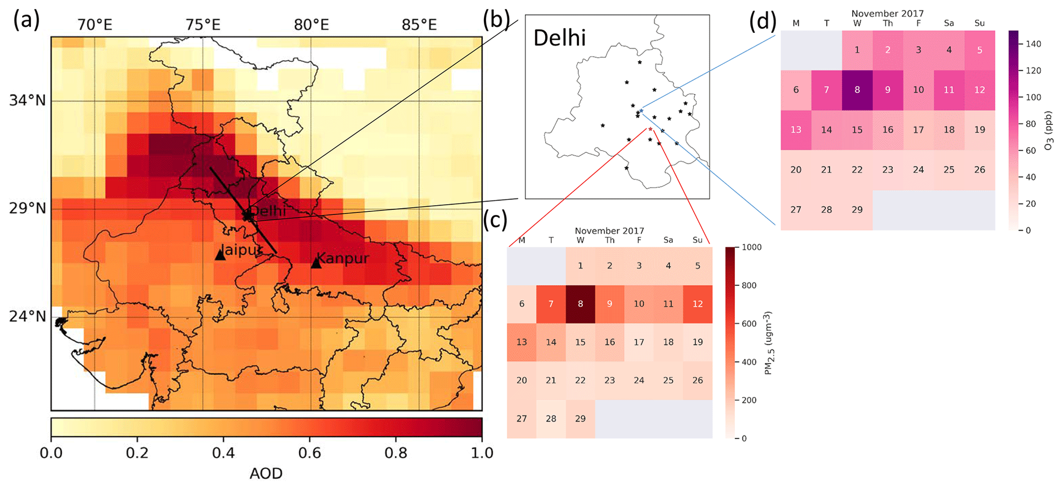
Figure 1WRF-Chem modeling domain, ground measurement stations, and observed air quality: (a) modeling domain and location of Delhi (∗) and AERONET stations at Jaipur and Kanpur (▴) and underlying VIIRS AOD (550 nm) averaged over November 2017; the black line also shows the path that was used for vertical cross-section analysis. (b) Location of CPCB stations (black stars); US Embassy station (red star); and North Campus, Delhi University (blue star). (c) Calendar map of averaged daily PM2.5 concentration measured at US Embassy, (d) Calendar map of averaged daily ozone concentration measured at North Campus, Delhi University.
Models usually underestimate the concentrations during extreme pollution periods unless they apply chemical data assimilation (Dekker et al., 2019; Kulkarni et al., 2020; Kumar et al., 2015b, 2020). Moreover, there are different input data in terms of chemical boundary conditions and fire emissions that can affect air quality modeling results (He et al., 2019). The main purpose of this study is to investigate the sensitivity of model predictions to the main inputs into the model. Prediction of extreme pollution events is important as such events have major impacts on people and also make a strong impression regarding the capabilities of models. However, extreme events are hard to predict because they are often heavily impacted by episodic emission sources. Here we take the approach of systematically exploring the impacts of different boundary conditions, dust, fire, and anthropogenic emissions on the predictions of the pollution episode in November 2017. A contemporary way to try to capture such events in a prediction model is to employ data assimilation (Kumar et al., 2020). The data assimilation results compensate for deficiencies in the inputs as well as for structural problems within the models. But the effectiveness of data assimilation improves as the capabilities of the forward model improves. Therefore, our results are also important for those using data assimilation to improve predictability. In this study, we use the Weather Research and Forecasting model coupled to Chemistry (WRF-Chem). Through a series of sensitivity experiments, we evaluate the impacts of biomass burning emissions coming from the Fire INventory from NCAR (FINN) and Quick Fire Emissions Dataset (QFED); chemical boundary conditions retrieved from the Model for Ozone and Related chemical Tracers (MOZART), the Community Atmosphere Model with Chemistry (CAM-chem), the Copernicus Atmosphere Monitoring Service (CAMS), and Modern-Era Retrospective analysis for Research and Applications Version 2 (MERRA-2) global models; the role of incorporating VIIRS active fire hot spots to improve biomass burning emission inventories and global models to improve chemical boundary conditions; and changes in dust and anthropogenic emissions on modeled PM2.5 concentration during November 2017. We also evaluate ozone predictions.
This paper is organized as follows. First, the WRF-Chem configuration; sensitivity experiments; and the observation datasets, including ground measurements and satellite data, are described. Then, after evaluating the model performance for the best experiment, the impacts of using different datasets as input data on modeled PM2.5 concentrations during November 2017 are analyzed and discussed.
2.1 WRF-Chem configuration
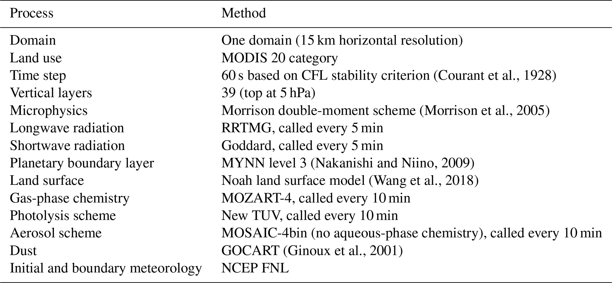
WRF-Chem is a numerical modeling framework that solves transport, chemistry, and physics of the atmosphere (Grell et al., 2005). The online interaction between meteorology, thermodynamic processes, and atmospheric chemistry makes it a powerful and reliable model in the community. WRF-Chem (version 4.0) with one domain centered on Delhi with a 15 km horizontal grid resolution and 39 vertical layers was used in this study. The domain was set to be big enough to include the northwest biomass burning and urban emission sources in the simulation process as they have been shown to be contributors to poor air quality in the region in previous studies (Amann et al., 2017). In the following, we present the model configuration for the base scenario (ID – FINN_VIIRS_7Xperiod2).
The National Centers for Environmental Prediction (NCEP) Global Forecast System (GFS) final analysis (FNL) 1×1∘ and 6 h spatial and temporal resolution meteorological fields (https://rda.ucar.edu/datasets/ds083.2/, last access: 22 January 2020) were used as initial and boundary conditions for the meteorology. CAM-chem data (Buchholz, 2019) with a horizontal resolution of 0.9×1.25∘ and 56 vertical levels provided chemical boundary conditions for gaseous species. MERRA-2 reanalysis data with 0.625×0.5∘ horizontal and 72 vertical model levels were used for aerosol species (Bosilovich et al., 2016). However, input data have uncertainties, and small uncertainties in nonlinear governing equations of numerical weather predictions can lead to non-negligible errors in results (Xiu, 2010). As a result, re-initialization of numerical weather prediction (NWP) models is suggested instead of free runs (Abdi-Oskouei et al., 2020). In this study, the model ran for 30 h each day starting at 00Z and the first 6 h of data was discarded to account for daily spin-up. Meteorological initial and boundary conditions and chemical boundary conditions were re-initialized daily at 00Z using global models. However other than for the first cycle in which global models provided initial chemical conditions data, chemical fields from the previous cycle were used as the next cycle's initial chemical conditions. Table 1 summarizes the WRF-Chem physical and chemical configuration options.
Studies have shown improvements for ozone simulations in Delhi using more complicated chemistry mechanisms like MOZART and CBMZ compared to simple mechanisms like RACM and RADM (Gupta and Mohan, 2015; Sharma et al., 2017). The MOZART gas-phase chemistry mechanism and the four-bin Model for Simulating Aerosol Interactions and Chemistry (MOSAIC-4bin) were used for modeling atmospheric chemistry and aerosol properties as suggested in previous studies over India (Kumar et al., 2015a). The MOZART version-4 mechanism was initially developed for global modeling of ozone and other tracers in the troposphere (Emmons et al., 2010). Although it includes 97 gas-phase and bulk aerosols, all monoterpenes, which are important in ozone chemistry, were initially lumped together. As a result, Hodzic et al. (2015) added a detailed treatment of monoterpenes and Knote et al. (2014) updated the isoprene oxidation scheme in the MOZART mechanism in WRF-Chem. MOSAIC is an aerosol model that considers a wide range of aerosol species that are important on a regional scale and treats the chemical and microphysical processes between them including nucleation, coagulation, thermodynamics and phase equilibrium, and gas–particle partitioning (Zaveri et al., 2008). Hodzic and Jimenez (2011) updated the secondary organic aerosol (SOA) formation mechanism, and the updated version is available in WRF-Chem for performing regional air quality modeling studies. MOSAIC-4bin, used in the current study, calculates all the above-mentioned aerosol physics and chemistry in four sectional aerosol size bins with the assumption that each bin is internally mixed and all the particles within a bin have the same chemical composition (Zaveri et al., 2008).
In India, both anthropogenic and natural sources have important impacts on air quality. Biomass and biofuel use in the residential sector for heating and cooking purposes make significant contributions to air quality in India (Conibear et al., 2018a; David et al., 2019; Venkataraman et al., 2018). Moreover, there are more than 1000 power plants and brick kilns in India that are major anthropogenic sources of SO2 and particulate matter, respectively (Guttikunda and Calori, 2013). Other than these industrialized sources, the literature shows that biomass burning (e.g. agricultural waste burning) contributes to 37 % of air pollution over the sub-continent (Kumar et al., 2015a). The Hemispheric Transport of Air Pollution (HTAP v2.2) (Janssens-Maenhout et al., 2015) emission inventory of 2010 with a 0.1∘ horizontal resolution, mapped to the MOZART–MOSAIC mechanism (https://www2.acom.ucar.edu/wrf-chem/wrf-chem-tools-community, last access: 1 December 2020), was used as the base anthropogenic emission inventory. Although the accuracy of urban anthropogenic emission inventories has significant effects on air quality modeling studies (Gupta and Mohan, 2015; Kumar et al., 2012; Sharma et al., 2017), the focus of this paper is to capture the air pollution due to regional sources; we did not use higher-resolution emission inventories for Delhi.
The Fire INventory from NCAR, version 1.5 (FINNv1.5), and Model of Emissions of Gases and Aerosols from Nature (MEGAN v 2.0.4) were used as biomass burning emission and biogenic emission inventories, respectively (Guenther et al., 2006; Wiedinmyer et al., 2011). However, other studies have noticed that uncertainties in FINN emissions can significantly modify the results (Kulkarni et al., 2020). Therefore, two modifications were applied to FINN data to provide better input data: filling missing fires using VIIRS fire radiative power (FRP) data and scaling the fire emissions (scaling procedure described in detail later). Liu et al. (2018) used FRP values to approximate the stubble burning areas affecting Delhi's air quality. In their statistical study, 99 % of post-monsoon FRP values were attributed to agricultural fires (Liu et al., 2018). In this study, we used FRP values to improve fire emissions. Specifically, we first regridded VIIRS 375 m resolution FRP data to our domain. Then at each hour, for all grid cells that have FINN emissions, we find the corresponding mean VIIRS FRP and perform a linear regression between FRP and emission flux. Afterwards, we apply the regression line parameters to VIIRS FRP for the grid cells that do not have any FINN emissions, to estimate the flux. It should be mentioned that all the available FRP data were utilized disregarding the retrieval's confidence level. Moreover, we used VIIRS instead of MODIS data as they provided higher-resolution active fire points data (375 m vs. 1 km), which is an important point for small fires. For example, no active fire points in the Moderate Resolution Imaging Spectroradiometer (MODIS) instrument were reported in 2018 post-monsoon for Uttar Pradesh (Kulkarni et al., 2020). Figure 9 shows more fire grid cells in the eastern IGP and central India when incorporating VIIRS data into the FINN inventory. We acknowledge that this technique is a first-order approximation and can have large errors as FINN is based on burned-area algorithms from MODIS-retrieved data; more detailed research is required to improve the idea.
Dust storms are an important natural pollution source that have caused many pollution events over some parts of India (Kumar et al., 2014a). The Goddard Global Ozone Chemistry Aerosol Radiation and Transport (GOCART) mechanism was used to calculate the threshold wind velocity and total dust emissions; about 70 % of the total mass was then distributed between different bins of the other inorganic (OIN aerosol component in WRF-Chem; OIN represents all primary inorganic PM) components in the model with the assumption that the rest are larger than PM10 (Zhao et al., 2010). This is based on a study in northern Africa, where Zhao et al. (2010) allocated about 1 % of the dust to bins with a diameter of less than 2.5 µm and 69 % of the dust in bin 4 (2.5–10 µm) and assumed the rest was bigger than 10 µm and would not remain in the atmosphere for an influential period.
Table 1Details of WRF-Chem physical and chemical setup configuration.
2.2 Sensitivity experiments
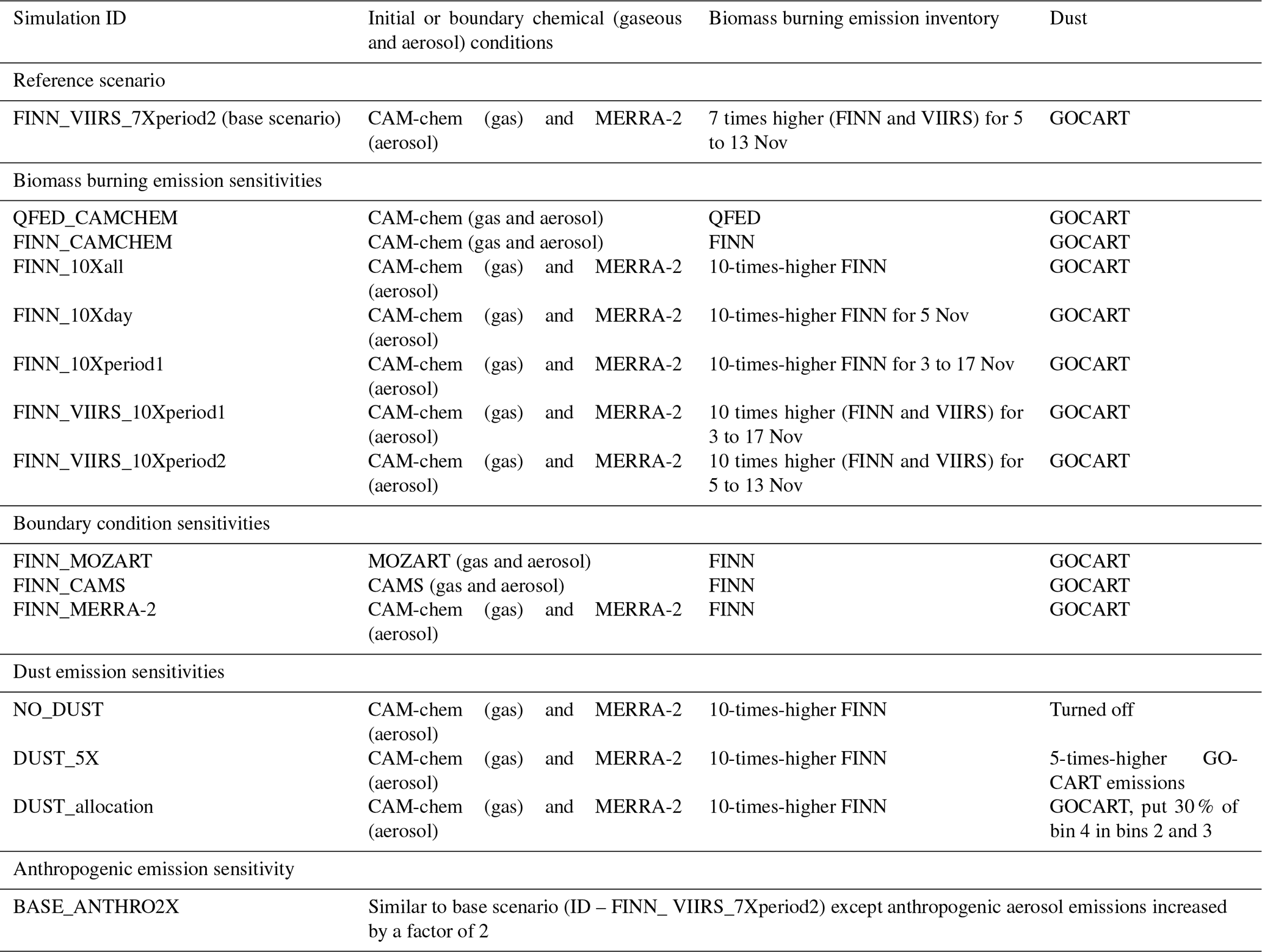
Three sets of experiments were performed to explore the impact of using different global data (as either boundary conditions or emissions) and dust emission formulations on PM2.5 and AOD predictions (Table 2). It should be mentioned that all the modeling options and other input data remained unchanged unless specified.
One set of experiments focused on the sensitivity of the predictions to biomass burning emissions. First, we compared the impacts of two different biomass burning emission inventories, namely FINN and QFED (Koster et al., 2015). Specifically, simulations using QFED (ID – QFED_CAMCHEM) and FINN (ID – FINN_CAMCHEM) were performed to understand the impact of different fire detection algorithms. When using QFED, it should be mentioned that we mapped total CO values to VOC species in the MOZART chemistry mechanism based on emission factors provided in the literature instead of using VOC emissions directly from QFED (Akagi et al., 2011). Second, we investigated whether FINN fire emissions were underestimated for all the days (ID – FINN_10Xall), some days (ID – FINN_10Xperiod1), or just 1 d before the pollution episode on 5 November (ID – FINN_10Xday). Then after modifying FINN using VIIRS FRP data, we performed a sensitivity test by changing the period for scaling fire emissions. Specifically, we scaled fire emissions for a 15 d period between 3 and 17 November (ID – FINN_VIIRS_10Xperiod1) and an 8 d period between 5 and 13 November (ID – FINN_VIIRS_10Xperiod2). We also evaluated the performance for a scaling factor of 10 in comparison with 7 (ID – FINN_VIIRS_7Xperiod2). Anthropogenic emissions over India also have high uncertainties (Saikawa et al., 2017). As a result, we studied how increasing the anthropogenic aerosol emissions by a factor of 2 affects the results (ID – BASE_ANTHRO2X).
Another set of experiments evaluated the impacts of chemical boundary conditions. Many global datasets can be used in regional air quality modeling. Simulations were performed using the global modeling systems CAM-chem (ID – FINN_CAMCHEM), MOZART (ID – FINN_MOZART), CAMS (ID – FINN_CAMS.), and a combination of CAM-chem for gaseous and MERRA-2 for aerosol species (ID – FINN_MERRA2). It is important to note that CAMS and MERRA-2 are reanalysis models and use observed data to improve the results. CAMS assimilates the MODIS and Advanced Along-Track Scanning Radiometer (AATSR) satellite instruments' AODs (Inness et al., 2019). MERRA-2 assimilates AOD from multiple sources including MODIS, the Multi-angle Imaging SpectroRadiometer (MISR), the Advanced Very High Resolution Radiometer (AVHRR), and the AErosol RObotic NETwork (AERONET) although assimilating some products has been stopped since 2014 (Randles et al., 2017).
Finally, simulations were conducted for various dust emission modifications. In one simulation, we turned off the dust emission option in the model (ID – NO_DUST), while in another simulation, we increased total dust emissions by factor of 5 to explore if dust emissions were underestimated in the model (ID – DUST_5X). Moreover, we changed the allocation of total dust to different bins of the MOSAIC module to see whether different allocation of aerosols can contribute to the observed extreme pollution in Delhi (ID – DUST_allocation). Specifically, we took 30 % from the fourth bin (2.5–10 µm) and allocated 25 % of it to the third bin (0.625–2.5 µm) and 5 % to the second bin (0.156–0.625 µm). More allocation to bins 2 and 3 was not considered, as it was not realistic of the large-size nature of dust aerosols. The FINN_10Xall scenario represents the simulation with the turned-on dust option (original allocation) in the model. Detailed results from experiments on boundary conditions and dust emissions can be found in the Supplement.
2.3 Observation data
The model performance was evaluated using ground measurements, spaceborne instruments, and global reanalysis data. Specifically, we used data collected by the CPCB over the domain for performing statistical analysis. They include stations over Delhi (19 stations), Rajasthan (10 stations), Haryana (4 stations), and Punjab (3 stations). No additional quality control filters, other than the ones by the CPCB (https://cpcb.nic.in/quality-assurance-quality-control/, last access: 20 February 2021), were applied. We evaluated the results after applying the filters proposed by other studies (e.g., Kumar et al., 2020); they had slight impacts on statistics (shown in the Supplement). PM2.5 data measured by a US EPA instrument at the US Embassy in Delhi were used as the reference station data. Level-2 VIIRS remote sensing instrument data on board the Suomi National Polar-orbiting Partnership (S-NPP) were used for comparing the spatial pattern of AOD and fire counts over the domain. Specifically, aerosol products with around a 6 km horizontal resolution based on the Deep Blue algorithm (Hsu et al., 2019) and 375 m active fire products based on the VNP14IMG algorithm (Schroeder et al., 2014) were used. There are only two AERONET stations in the domain (Fig. 1a). AERONET data at these two sites confirmed the reliability of VIIRS-retrieved data (Fig. S5). MERRA-2 gridded data were also used to evaluate the model performance. MERRA-2 reanalysis is based on the assimilation of many meteorological data and the assimilation of AOD from multiple satellites (Gelaro et al., 2017). The on-ground continuous-monitoring station guidelines state that instruments should sample at heights between 3–10 m. Irrespective of this condition, some of the CPCB stations are placed on top of buildings with a restricted clean flow of air (personal inspections). While we observed little impact of this situation on the concentrations in a well-mixed layer, a meteorological parameter like wind speed data can show erratic behavior. As a result, we used MERRA-2 meteorological data to evaluate the WRF-Chem simulations using 10 m wind speed and direction, 2 m temperature, and surface water vapor mixing ratio variables.
We also compared MERRA-2 AOD (at 550 nm) and PM2.5 predictions with WRF-Chem results to evaluate how the assimilation of AOD affected the predictions. The MERRA-2 PM2.5 was based on the mass mixing ratios of black carbon, organic carbon, dust, sea salt, and sulfate. Since ammonium concentration is not available, it is common in the literature to assume that sulfate ion will be completely neutralized by ammonium and form ammonium sulfate, and therefore a factor of 1.375 was assumed in calculating inorganic aerosol concentrations (Buchard et al., 2016; He et al., 2019; Provençal et al., 2017). On the other hand, the literature suggests organic carbon concentration should be multiplied by 1.4 to compensate for other missing organic compounds to estimate the organic mass (Buchard et al., 2016; Chow et al., 2015; He et al., 2019; Provençal et al., 2017; Turpin and Lim, 2001). However, Turpin and Lim (2001) argued that this scaling factor should be 2.6 for biomass burning particles; we used 2.6 according to our studied time period and potential black carbon sources:
where BC is black carbon, OC is organic carbon, SO4 is sulfate, DUST is dust, and SS is sea salt concentrations. As dust and sea salt data are reported in multiple bins, different bins should be used for different particle diameters.
The metrics we used to assess the performance of the simulations were the root mean square error (RMSE), mean error (ME), normalized mean bias (NMB), normalized mean error (NME), and correlation coefficient (R) as defined in the Supplement (Emery et al., 2017, 2001). Since low values can have significant impacts on normalized values, which are used in mean normalized metrics, normalized mean values are better metrics and used in this study (Emery et al., 2017).
3.1 Model performance
Our analysis comparing different simulations revealed that the FINN_VIIRS_7Xperiod2 scenario had the best statistical performance of the configurations studied. This scenario is called the base scenario, and we evaluate it in this section. Performance of the base model in capturing the meteorological parameters was evaluated using MERRA-2 data for 10 m wind speed and direction, 2 m temperature, and the surface water vapor mixing ratio. Figure 2a–d show these comparisons at the location of the US Embassy in Delhi (28.59∘ N, 77.19∘ E). The model was able to capture the general diurnal trend for all these variables and the sharp shift in wind direction between 13 and 17 November, after the extreme pollution episode. Negatively biased wind speed with an ME of 1.1 m s−1 and RMSE of 1.28 m s−1 shows the model generally underestimated wind speed, and it was most predominant between 17 and 25 November. Figure 2c shows the model did not accurately capture nighttime 2 m temperature minima but captured the maximum values with an overall overestimated ME of 3.52 ∘C and RMSE of 4.01 ∘C. The wind speed satisfied the benchmark RMSE value of 2.0 m s−1, while temperature was higher than the targeted ME goal of 2.0 ∘C (Emery et al., 2001). The representation error plays an important role in evaluating results due to different horizontal resolutions in the model and MERRA-2 dataset ( vs. 0.625×0.5∘), specifically in urban areas. For instance, the same statistics for a rural area in Rajasthan (27.0∘ N, 73.0∘ E; not shown) have smaller biases and are compliant with benchmark values (RMSE of 0.99 m s−1 for wind speed and ME of 1.08 ∘C for 2 m temperature). For the water vapor mixing ratio the model clearly captured the daily variations, especially the increase after the pollution episode (13 November). However, it showed a very sharp day-to-night shift during the pollution episode days. The spatial performance of the model averaged over November during daytime hours (08:00 to 18:00 local time) is shown in Fig. 2e–j. The sharp gradient between the Himalayan and IGP regions in the northeast, the gradient between land and sea in the southwest, and the slight gradient between different land types in the northwest of the domain for both 10 m wind speed and 2 m temperature were captured well. Overall, the model was able to capture the general daily variations and spatial trends when compared to MERRA-2 data.
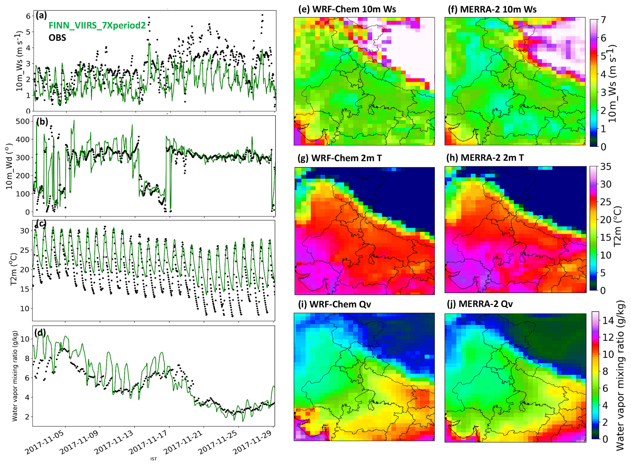
Figure 2Temporospatial meteorological performance of base scenario simulation: time series of simulated (green line) and MERRA-2 (black dots) hourly (a) 10 m wind speed, (b) 10 m wind direction, (c) 2 m temperature, and (d) surface water vapor at US Embassy coordinates. (e, f) Averaged daytime (08:00–18:00 LT) 10 m wind speed maps of model (e) and MERRA-2 (f). (g, h) Averaged daytime (08:00–18:00 LT) 2 m temperature maps of simulations (g) and MERRA-2 (h). (i, j) Averaged daytime (08:00–18:00 LT) surface water vapor mixing ratio (g kg−1) maps of model (i) and MERRA-2 (j).
Figure 3 shows spatial distribution of the base scenario, VIIRS data, and the bias for the 550 nm AOD, averaged over all the days in November with 5 November as a day with intensive fire emissions and 24 November as an illustrative day after the extreme pollution episode. The model showed high AODs over Delhi and Punjab, confirming satellite data. Moreover, AODs were high over the western IGP, close to major fires of Punjab, with a gradual gradient towards eastern and central India. Dust emission sources at the border of Pakistan also led to high AODs although they did not affect Delhi as discussed in the Supplement. In general, the model underestimates AOD over the IGP and overestimates it elsewhere. WRF-Chem predicted the averaged AOD over the whole domain for November 2017 to be 0.58 (±0.4), while VIIRS data showed 0.43 (±0.26). AOD maps for 5 November show the model generally underestimated AOD values for the entire IGP region, except for Punjab. Moreover, the model underestimated aerosol loadings over central India. Other studies have reported biased-low AOD and corresponding PM2.5 concentrations over other polluted regions (He et al., 2019; Song et al., 2018). On the other hand, 24 November represented a day with no significant fire emissions. The model did a good job capturing AOD values in the central parts of India and around Delhi. However, the model missed high AOD values in the eastern IGP. MERRA-2 data also did not show high AODs over the western border with Pakistan and did not capture extremely high AODs over Punjab, although they showed AOD enhancements (Fig. S6).
Figure 4 shows time series of modeled, MERRA-2 product, VIIRS-retrieved, and observed AOD at the AERONET stations (location shown in Fig. 1). AOD values at Kanpur, a station in the eastern IGP, were more than 1.0 before the pollution episode, reached up to 2.0 during the episode days, and decreased to values of between 0.5 and 1 for the rest of the days. The model captured the general trend although missed high AODs between 9 and 13 November, while MERRA-2 successfully captured the AOD trend through the whole month, including days with enhanced AOD values. This shows that AOD assimilation in MERRA-2 significantly improves AOD predictions. At Jaipur, located in the southern IGP, the model overestimated AOD for the first 5 d of November. During the pollution episode days, the model is biased high compared to MERRA-2 and VIIRS retrievals. AERONET data showed low AOD values before the pollution episode but did not report values during the pollution episode. This suggests, as one possibility, that PM concentrations were too high during this period for the instrument to retrieve data. After the pollution period, AOD values were lower than 0.5, showing relatively low PM concentrations. In general, MERRA-2 showed better performance in terms of NMB (Kanpur −1.3 % and Jaipur −20.1 %) compared with our model (Kanpur: −27.4 % and Jaipur: +29.9 %). Comparing averaged AOD with VIIRS retrievals for the BASE_ANTHRO2X scenario showed lower bias over the IGP (Fig. S7). These results show the need for improved estimates of biomass burning as well as anthropogenic emissions. We also looked at the Ångström exponent (AE) at Jaipur and Kanpur to understand if the model captured the mode of the particles (Fig. S8). Over Jaipur the model is biased high compared to AERONET data (NMB 30 %) and shows more finer aerosols in the model. After 20 November, both AERONET and VIIRS retrievals suggest the dominance of coarser aerosols, while the AE for the model does not follow the same trend. However, the modeled PM2.5 PM10 ratio shows more coarse aerosols compared to the rest of the month (Fig. S9). Over Kanpur, the model AE is biased high (NMB: 50.8 %). On the other hand, the model shows closer AE values to VIIRS retrievals. For example, both the model and VIIRS retrieval show similar reduction in the AE on 8 and 9 November. Kumar et al. (2014b) also reported slight AE overestimation in WRF-Chem during a pre-monsoon dust storm at Kanpur and Jaipur. Furthermore, the model and AERONET have a variational trend while MERRA-2 is smooth during the whole month at both Jaipur and Kanpur.
Figure 5a shows time series plots of base scenario and observed PM2.5 concentration at the US Embassy station. Observed values were high throughout the month on the order of 200 µg m−3 with diurnal variations due to changes in the mixing heights. The extreme pollution episode began on 7 November, when PM2.5 concentrations increased to more than 800 µg m−3. On 8 November, the values increased even more to about 1000 µg m−3. PM2.5 concentrations started decreasing on 9 November and continued decreasing through 10 November. However, values increased again and were high between 11 and 13 November. Afterwards, they returned to ∼200 µg m−3 for the rest of the month. The model accurately captured the magnitude and diurnal cycle for PM2.5 for non-episodic days. Moreover, the model was able to see the sharp increase in concentration in the beginning of the episode starting from 7 November with reported PM2.5 concentrations of ∼650 µg m−3. This sharp increase was captured after incorporating VIIRS data into FINN emissions accompanied by scaling the emissions by a factor of 7. In fact, increased emissions from fires in agricultural fields in the northwest on previous days and favorable northwesterly winds, as shown in Fig. 2, explain this concentration hike. However, the model underestimated the concentrations for the next 3 d. Then, the model captured the second enhancement. Although wind direction showed good agreement with the MERRA-2 dataset and wind speed was biased low and even more favorable for stagnant conditions, modeled PM2.5 concentrations had a large negative bias for the period between 8 and 10 November. This suggests either low local anthropogenic emissions within Delhi or some missing pollution sources upwind of Delhi that were not included in the emission estimates led to underestimation.
Dekker et al. (2019) studied CO concentrations during November 2017 using satellite observations, and they reported low emissions as one of the reasons for large negative concentration biases, although they proposed unfavorable meteorological conditions as the main reason for high CO concentrations in Delhi, between 11 and 14 November. Moreover, Cusworth et al. (2018) reported that MODIS-based biomass burning emission inventories miss many small fires over India. Beig et al. (2019) concluded that long-range-transported dust coming from the Middle East was a major source for this extreme pollution episode. Figure 5a shows that MERRA-2 did not capture high surface PM2.5 concentrations after 8 November. Navinya et al. (2020) reported that MERRA-2 underestimates PM2.5 over India, especially during the post-monsoon season. More discussions on the extreme pollution episode are provided in the following section.
Starting on 13 November, the modeled concentrations went down as winds shifted to easterlies and wind speed increased. Beig et al. (2019) found PM2.5 concentrations after the pollution episode were lower compared with similar periods in previous years. Thereafter, the concentrations went back to values for Delhi before the episode. The model did a fairly good job of capturing the trend during non-episode days (Table S4). Increasing anthropogenic emissions (ID – BASE_ANTHRO2X) on simulation results overestimated PM2.5 concentrations in the US Embassy location during non-episode days (Fig. S7).
Figure 5b and c show the averaged PM2.5 maps for all the hours over the studied region in the base simulation and MERRA-2 dataset. The model was able to capture higher concentrations over northwestern India and the border with Pakistan where agricultural fire and dust emissions play the most important role for extreme pollution episodes over IGP. However, the model showed higher values than MERRA-2 over southern Punjab, a region with high biomass burning emissions (Kulkarni et al., 2020). Since MERRA-2 assimilates satellite AOD data as its major aerosol forcing, it will not be able to capture high concentrations if satellite retrieval algorithms miss corresponding high AODs.
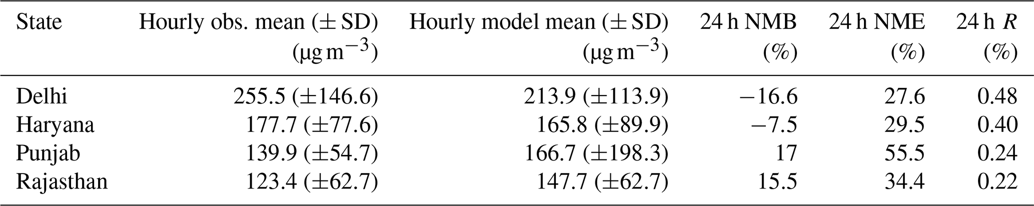
Figure 5b and c also show that the model was biased high over central India and biased low over the eastern IGP. These results indicate improving emissions in the eastern IGP can significantly improve the simulation results. Conibear et al. (2018a) also reported limited success of models to capture the spatial variability in PM2.5 over India in 2016, specifically during winter. Table 3 provides statistics for 24 h averaged PM2.5 concentrations for the base scenario simulation for Delhi and its western states. Statistics for Delhi show an NMB of −16.6 %, which passes the “criteria” benchmark of 30 %, while an NME of 27.6 % shows better performance and complies with the benchmark “goal” of 35 % for the whole month (Emery et al., 2017). A correlation coefficient of 0.48 is also higher than the benchmark criterion of 0.4. Statistics significantly improve after excluding the 4 extremely polluted days between 7 and 10 November and all are within benchmark goals (Table S4). Kumar et al. (2020) assimilated MODIS AOD into WRF-Chem in order to improve the air quality forecasts over Delhi. In their study, the mean bias for first-day forecast of PM2.5 concentration decreased from −98.7 to −13.7 µg m−3. They also showed that the RMSE decreased from 167.4 to 117.3 µg m−3. Our results from the base scenario (mean bias of −42.38 µg m−3 and RMSE of 118.47 µg m−3) show comparable results to the data assimilation technique, although both models are still biased low.
Statistics for the state of Haryana (4 stations) show good performance (NMB of −7.5 % and correlation coefficient of 0.4). The model was biased high for Rajasthan (10 stations, NMB 15.5 %) and Punjab (3 stations, NMB 17 %). The model slightly overestimated PM2.5 concentrations during the episode days in Rajasthan but captured the concentrations during the rest of the month (Fig. S10). In Punjab, measured data did not report PM2.5 enhancement during the extreme episode, while the model showed very high concentrations after scaling fire emissions by a factor of 7. However, VIIRS satellite images (e.g., Fig. 9d) clearly show massive agricultural fires in this state during November, and its signals were expected in the measured data. The overall scatterplots including the averaged values for each state show good spatial performance of the base scenario (Fig. S11).
Although different meteorological parameters can be responsible for the biases, accuracy of anthropogenic emissions is important. For example, recent local anthropogenic emission inventories developed for Delhi have higher particle emissions than in the regional inventory used in this study, which impacts modeled PM2.5 concentrations for typical days (Kulkarni et al., 2020). We conducted the BASE_ANTHRO2X scenario to investigate the effect of uncertainties in the anthropogenic emissions. This scenario increased PM2.5 concentrations in Delhi to up to ∼150 µg m−3, which led to overestimation (in contrast to underestimation in the base scenario) on many of the non-episode days (Fig. S7). Although this scenario did not help in capturing the high concentrations during the episode, it confirms the need for better anthropogenic emissions. On the other hand, it reduced the bias over the IGP (Fig. S7). These results point out the need for best estimates of both anthropogenic and biomass emissions. Maps also show that averaged PM2.5 concentrations over most of India were higher than the air quality standard.
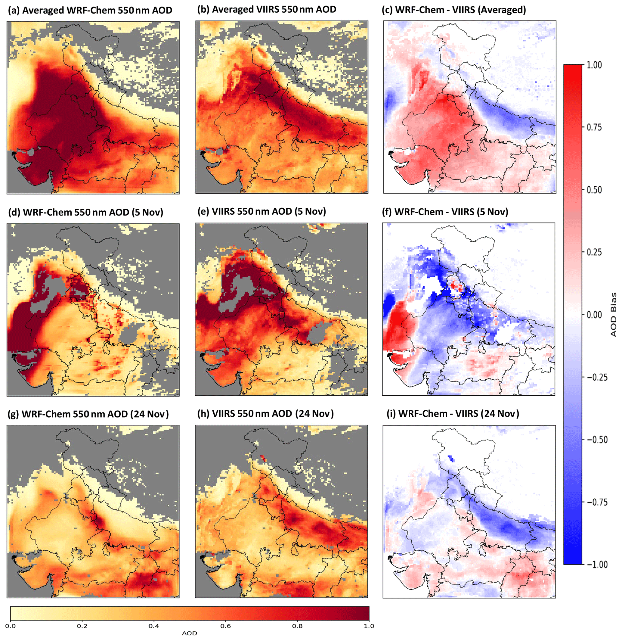
Figure 3Spatial distributions of AOD at 550 nm averaged over the whole of November (a–c), 5 November (d–f), and 24 November (g–i). WRF-Chem maps represent base scenario results. Differences between model and VIIRS are also shown.
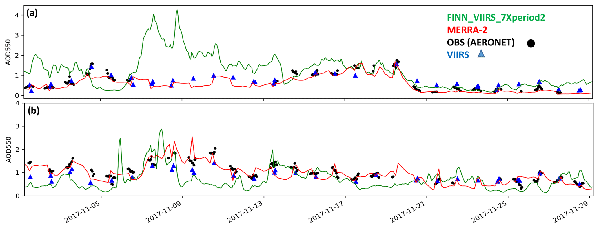
Figure 4Time series of modeled (green line), VIIRS-retrieved (blue triangles), MERRA-2 (red line), and AERONET (black dots) AOD at 550 nm during November 2017 at (a) Jaipur and (b) Kanpur.
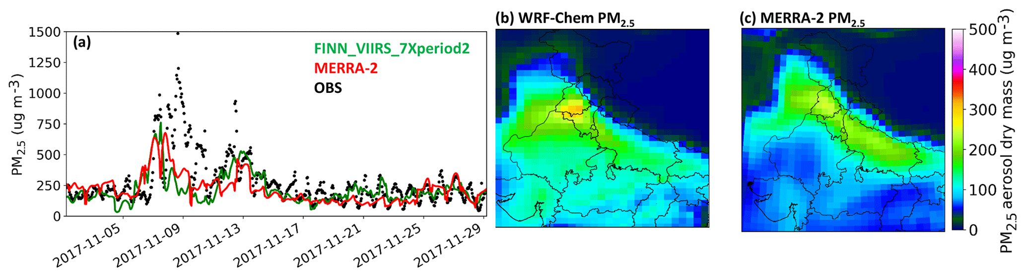
Figure 5Temporospatial air quality performance of base scenario simulation: (a) time series of simulated (green line), MERRA-2 (red line), and ground measurement (black dots) hourly PM2.5 concentration at US Embassy coordinates. (b, c) Hourly averaged PM2.5 concentration maps of model regridded to MERRA-2 resolution (b) and MERRA-2 (c).
Table 3Mean (± standard deviation), normalized mean bias (NMB), normalized mean error (NME), and Pearson's correlation coefficient (R) averaged for all CPCB stations in different states during November 2017. Model values are for the base scenario (FINN_VIIRS_7Xpeiod2). Mean values are for hourly data, while NMB, NME, and R relate 24 h averaged values.
3.2 Extreme-pollution-episode analysis
Figure 6a shows the box-and-whisker plots for daily PM2.5 concentration for the base scenario and all of the CPCB stations in Delhi. Over all CPCB stations in Delhi, 24 h averaged measured values for PM2.5 ranged between 133 and 664 µg m−3, which is about 2 and 11 times higher, respectively, than the India 24 h standard value of 60 µg m−3. The model showed overall good performance for daily PM2.5 concentrations for days without extreme pollution (Table S4; NMB of −2.44 and R of 0.7) and followed the observed trend in the extreme pollution episode (Fig. 6), which suggests the overall meteorology and transport patterns were captured by the simulations. However, the model started the episode on 6 November and significantly overestimated the concentrations. The model captured the median for 7 November very well, although measured values span a wider range. The model missed the high concentrations on 8 November, which led to underestimations on 9 and 10 November, as well, regardless of capturing the decreasing trend. However, the model was able to simulate the second wave of the episode starting on 11 November and accurately captured the median and range of PM2.5 concentrations on 12 and 13 November. It is important to point out that the underestimation of PM on 9 and 10 November persisted for all of the sensitivity cases performed. This suggests the transport in the model during these days missed highly polluted source regions or significant emission sources for these days were not included in the inventories or both.
Back trajectories can be used to provide insights into modeled concentrations during the extreme pollution episode. Back trajectories were calculated for releasing 10 000 air parcels at 100 m above ground level and over eastern Delhi using the FLEXible PARTicle dispersion model (FLEXPART) with inputs from WRF-Chem output (Brioude et al., 2013). Figure 7 shows 72 h mean back trajectory maps for 6, 7, 8, 9, and 10 November. The releasing times are 00:00 (red line; denoted by the suffix _00 in the text below) and 12:00 (blue line; denoted by the suffix _12 in the text below) UTC on each day. Also plotted are the fire (gray line) and anthropogenic (black line) emissions along the trajectory. The model started to build up PM2.5 concentrations on 6 November and was biased high (Fig. 6a). Back trajectories for 6 November_00 show PM2.5 concentrations were majorly due to anthropogenic emissions (Fig. 7a). However, 6 November_12 trajectories in Fig. 7c show a spike in fire emissions at previous hours (backward hours 5 and 30), which immediately led to high PM2.5 concentrations. Moreover, trajectory paths for this day reveal that emissions belonged to fires east of Delhi. Figure 9 shows that the fires east of Delhi in the base scenario are due to incorporating VIIRS data into the fire emissions. Therefore, high-biased PM2.5 concentration may be related to the scaling factor applied to eastern Delhi fires. On 7 November, the model perfectly captured the PM2.5 median (Fig. 6a). Back trajectories for 7 November_00 (Fig. 7d, e) show the beginning of a shift in wind direction and PM2.5 concentration was exclusively due to fire emissions on 5 November (backward hour 40). Compared to 7 November_00, fire emission footprints for 7 November_12 trajectories are smaller, while local anthropogenic emissions are higher (Fig. 7f). Back trajectories for 8 November show the northern parts' contribution for both releasing times, although trajectories for 8 November_00 crossed through central parts of Punjab. Moreover, local anthropogenic emission sources affected 8 November_00 trajectories. The model underestimated PM2.5 concentrations on 8 November, which can be partly related to errors in transport as the trajectories for 8 November_12 crossed eastern parts of Punjab. However, other physical processes or lower anthropogenic emissions can also be responsible for low-biased concentrations. Delhi's air quality for 9 November_00 was still being affected by northern parts, while trajectories for 9 November_12 shifted towards the east. Since trajectories for 9 November do not show any fire or anthropogenic emission pulse, the model missed either the dynamics of that day or emission sources. Trajectories for 10 November show eastern flow, again, and no fire emission contribution.
To further understand the regional-scale transport of the smoke plumes, we plotted a cross section of PM2.5 over the path from Punjab through Delhi (Fig. 8, path line shown in Fig. 1). PM2.5 concentrations showed typical values for 5 November_00 although they still exceeded the standard limits. For 5 November_12, concentrations significantly increased over Punjab area because of fires, and the winds brought them on a path towards Delhi. The Punjab's smoke had not yet completely crossed Delhi on 6 November as back trajectories for 00:00 and 12:00 UTC hours also showed the effects of anthropogenic emissions and fires in eastern Delhi. On the other hand, a significant amount of smoke was above the boundary layer as shown in the 6 November_12 panel. Due to shifting winds on 7 November (as shown in Fig. 2), the smoke upwind of Delhi blew over Delhi and led to extremely high concentrations. Although the model captured the median on 7 November, it missed the maximum extent of observed values. Cross sections on 8, 9, and 10 November show Punjab's residual smoke in the boundary layer, while we saw the model underestimated PM2.5 concentrations on these days. Measured PM2.5 concentrations over Delhi show a decreasing trend between 8 and 10 November (Fig. 6). Vertical profiles for the base scenario also show the model captured a high biomass burning emission period on 6 November (Fig. 12). However, it also showed high amounts of smoke above the planetary boundary layer (PBL). Cross sections for 11 to 14 November can be found in the Supplement (Fig. S12). These results suggest that plume rise in the model released the emissions too high or the model did not mix the smoke down fast enough. Using an ECMWF map, Vijayakumar et al. (2016) showed agricultural fires can transport particles via the upper troposphere and subside over Delhi. Social reasons can also be important as the first reaction of people during hazy days is to drive to work which directly (exhaust emissions) and indirectly (road dust) worsens air pollution.
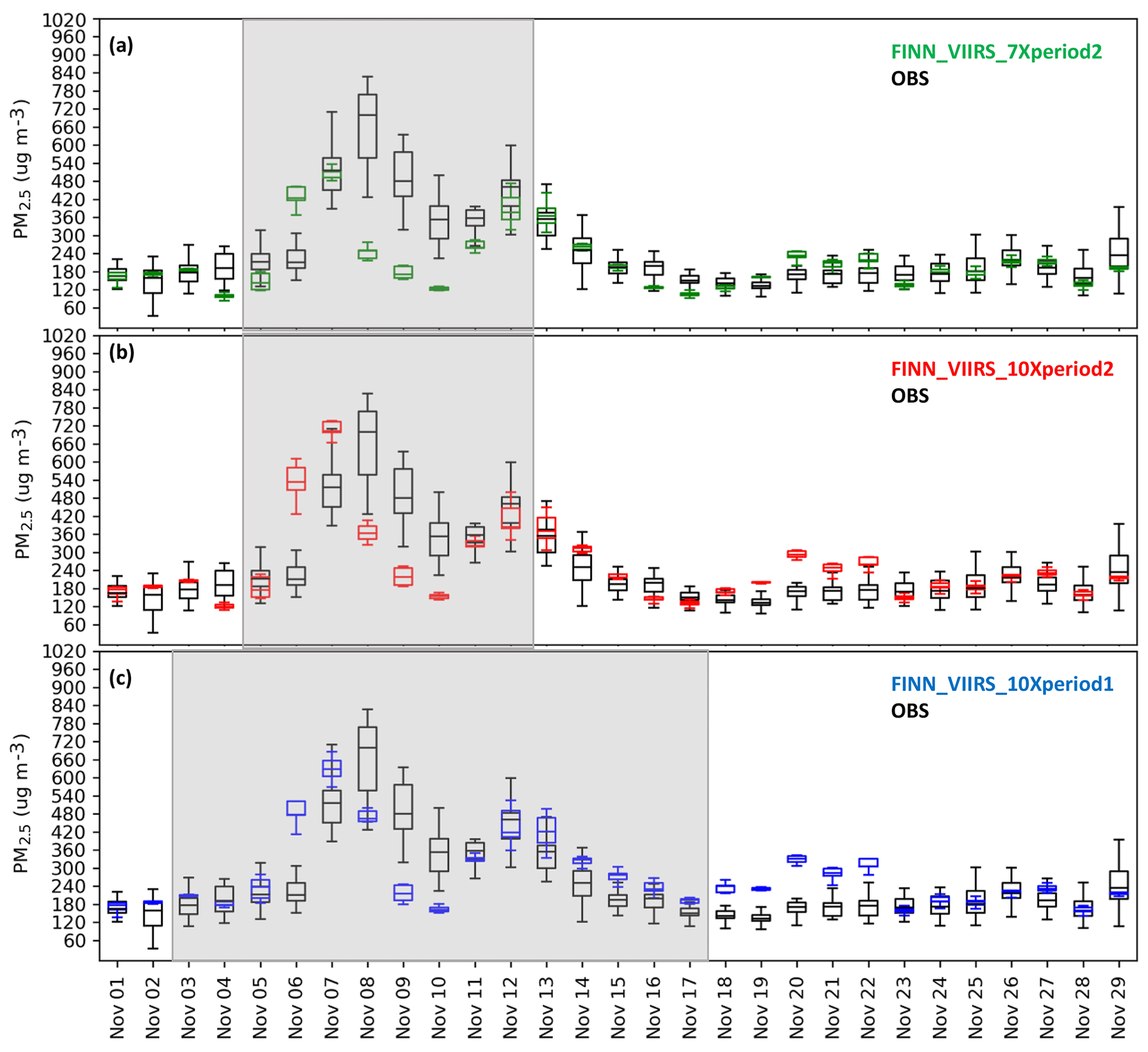
Figure 6Box-and-whisker plots of observed (black) and modeled daily PM2.5 concentration averaged over all CPCB stations in Delhi: (a) FINN_VIIRS_7Xperiod2, (b) FINN_VIIRS_10Xperiod2, and (c) FINN_ VIIRS_10Xperiod1. Shaded area shows the time window when biomass burning emissions were increased.
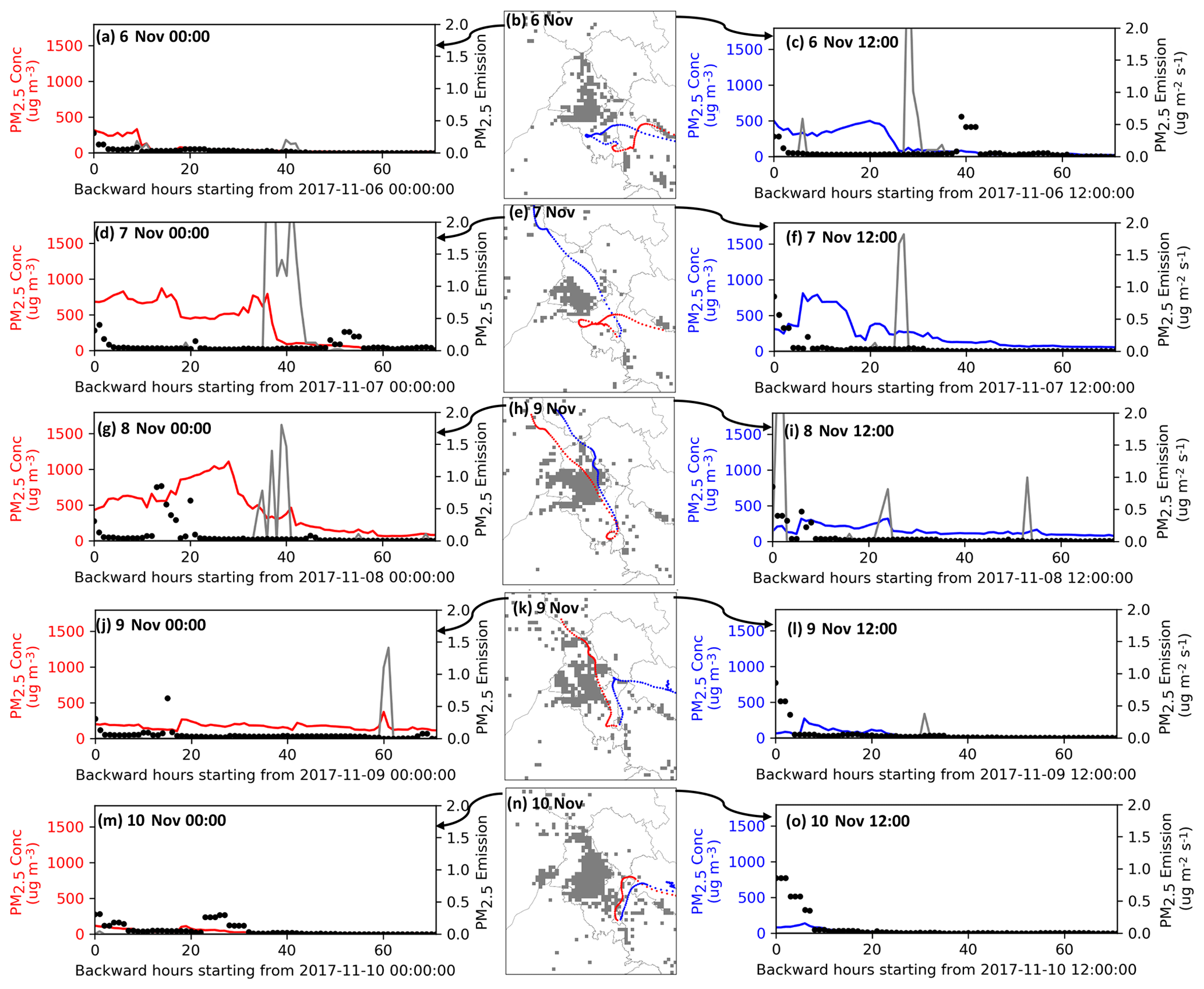
Figure 7Back trajectory plots of PM2.5 concentration (base scenario) on different days for 72 h: in each row, the map shows the back trajectory path for the mass mean location for releasing 10 000 particles over eastern Delhi at 00:00 UTC (red line) and 12:00 UTC (blue line), where the underlying map shows FINN grid cells on that day. Time series show PM2.5 concentrations (primary y axis) and emissions (secondary y axis) for anthropogenic (black dots) and FINN (gray line) inventories along the path. Dates are (a–c) 6 November, (d–f) 7 November, (g–i) 8 November, (j–l) 9 November, and (m–o) 10 November. The times 00:00 and 12:00 UTC denote 05:30 and 17:30 local time, respectively.
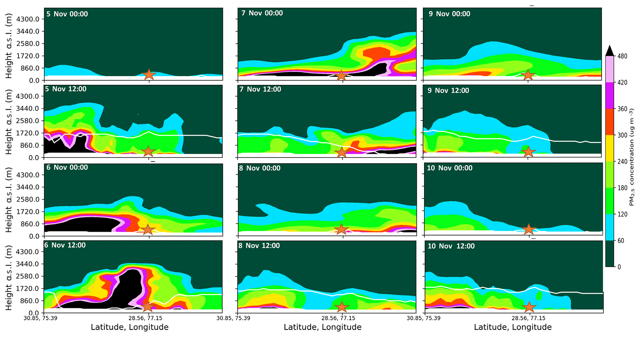
Figure 8Vertical cross section of PM2.5 concentration along the path shown in Fig. 1 for the days between 5 and 10 November. For each day, two snapshots are shown at 00:00 UTC (05:30 local time) and 12:00 UTC (17:30 local time). The orange star shows the location of Delhi on the path. The white line shows the PBL height across the path.
3.3 Sensitivity to changes in biomass burning emission inventories
Biomass burning emissions used in the base scenario in order to capture the extreme pollution episode were tuned after exploring how these inventories influenced PM2.5 concentrations (Table S3). First, we looked at two different emission inventories based on different methodologies and horizontal resolutions, specifically, FINNv1.5 and QFEDv2.5r1. Both inventories rely on MODIS data; FINN is based on active fire points and estimates of burned area, whereas QFED uses an FRP approach (Pan et al., 2020). Figure 9 shows the grid cells with biomass burning emissions based on QFED (panel a), FINN (panel b), and FINN_VIIRS composition (panel c), used in the base scenario, accompanied by active fire points seen by VIIRS (panel d) based on the Fire Information for Resource Management System (FIRMS) product for 5 November. It shows FINN captured more fire points in the domain although missed some in the eastern IGP and central India while QFED missed almost all of the fire points in Punjab on that specific day. As a result, the QFED simulation did not show any major signal for PM2.5 concentration on 7 November, whereas the experiment using the FINN inventory (ID – FINN_CAMCHEM) followed the measured start of the episode period, regardless of its low-biased PM2.5 concentrations (Fig. S13). In general, results using the QFED inventory had worse statistics (Fig. 11 and Table S3), which is mostly due to the inability of the inventory to capture the fire points over the domain, and it can be attributed to both the technique and the resolution as QFED data have a ∼10 km resolution, whereas FINN data have a ∼1 km resolution. Pan et al. (2020) found high uncertainty between different biomass burning emission inventories over Southeast Asia. They showed FINN is, in general, a better dataset for tropical regions as its 2 d continuous fire emissions compensate for the lack of daily MODIS coverage used in QFED (Pan et al., 2020; Wiedinmyer et al., 2011). Dekker et al. (2019) increased the GFAS biomass burning emission inventory by a factor of 5, did not see any improvement to CO simulation, and reported about a 2 % contribution from fires to Delhi's air quality. Our results confirm that FINN provides better biomass burning emissions for India for this period and shed light on the importance of choosing a proper biomass burning emission inventory for a specific domain.
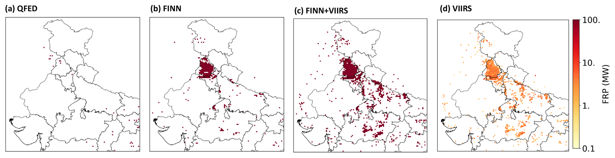
Figure 9Spatial fire coverage in different datasets for 5 November: (a) QFED fire grid cells; (b) FINN fire grid cells; (c) FINN fire grid cells, missing points filled with VIIRS; and (d) VIIRS active fire points and corresponding FRP values.
However, the signals from the simulation using the FINN biomass burning emission inventory were not high enough as it recorded a maximum concentration of 400 µg m−3 while the corresponding measured value was 680 µg m−3. Since observation data are sporadic over India and there were not many ground measurement stations available, sophisticated techniques such as inversion modeling were not feasible (Saide et al., 2015). As a result, manual tuning of the emission data was performed. The first attempt was to understand if FINN was required to be increased for the whole month; a 15 d period around the episode; or just on 5 November, which had many fire points in Punjab (Fig. 9). Figure 10 shows PM2.5 time series averaged over all CPCB stations based on these scenarios. Increasing FINN emissions for the whole month (ID – FINN_10Xall) led to an overestimation in the first 5 d of November, but it significantly helped in capturing high peaks on 7 and 8 November. Moreover, it increased the concentrations on 12 and 13 November regardless of missing the peaks. However, it did not show any improvements between 9 and 12 November, which suggests that the included fires did not influence Delhi's air quality during this period. On the other hand, increasing FINN emission data by a factor of 10 for all days led to very high PM2.5 concentrations on later days (20–27 November). This showed that FINN data were not systematically biased low. In other words, these results suggest that the FINN algorithm underestimated the magnitude of only some fires emission amounts. Some studies have shown that thick fires can be identified as clouds in retrieval algorithms (Dekker et al., 2019; Huijnen et al., 2016). As another experiment, we increased FINN emissions only on 5 November since that day had original high values in the inventory (ID – FINN_10Xday). This experiment resulted in better PM2.5 concentrations in the last third of November. However, it captured only the high concentrations of 7 November and missed the peak of 8 November as well as underestimated concentrations on some other days including 13 November. Finally, we multiplied the fire emissions by 10 for a 15 d period between 3 and 17 November (ID – FINN_10Xperiod1). In this way, we were able to capture the peaks on 7 and 8 November, see major contributions between 12 and 14 November, and see realistic values between 19 and 27 November. It should be mentioned this 15 d period was chosen arbitrarily and better scaling factors could be achieved by implementing tracers in the model, which is beyond the scope of this paper.
Although this experiment significantly improved the statistical performance for the CPCB stations, the model spatially underestimated concentrations over the eastern IGP (Fig. S14). Moreover, we observed lower fire grid cells in the FINN inventory compared to VIIRS active fire points (Fig. 9). As a result, we tested how incorporating VIIRS data into FINN in order to fill missing fire grid cells would improve the results. Figure 10 shows how incorporating VIIRS data improved the performance on 12 and 13 November (ID – FINN_VIIRS_10Xperiod1). However, the model started the episode too early on 6 November and overestimated PM2.5 concentrations after the episode. This suggests that the 15 d period for increasing FINN emissions could be too long; we then changed the scaling period from 15 to 8 d between 5 and 13 November (ID – FINN_VIIRS_10Xperiod2). This modification led to higher PM2.5 concentrations on 7 November as Fig. 6 shows. Moreover, the model was still biased high on after-episode days, which led to choosing the increasing factor of 7 (ID – FINN_VIIRS_ 7Xperiod2) as our best experiment.
Figure 11a shows a Taylor diagram for hourly PM2.5 concentrations based on the studied experiments, representing their statistical performance, for all the days in November. It shows that switching between different experiments mostly improved the standard deviation values. The QFED_CAMCHEM experiment had the lowest standard deviation but missed high PM2.5 concentration values. On the other hand, three experiments using VIIRS-integrated fire emissions had standard deviations closer to the measured value. Although the base scenario had good statistical metrics, the standard deviation and correlation coefficient were lower compared to the other two VIIRS-included and BASE_ANTHRO2X scenarios for all the days. The reason for this is that overestimation of other scenarios for 7 November and after-episode days compensates for underestimation between 8 and 10 November. Figure 11b shows the same variables for all the days except 8, 9, and 10 November. It shows that the base scenario had the best statistical performance for days without extreme pollution.
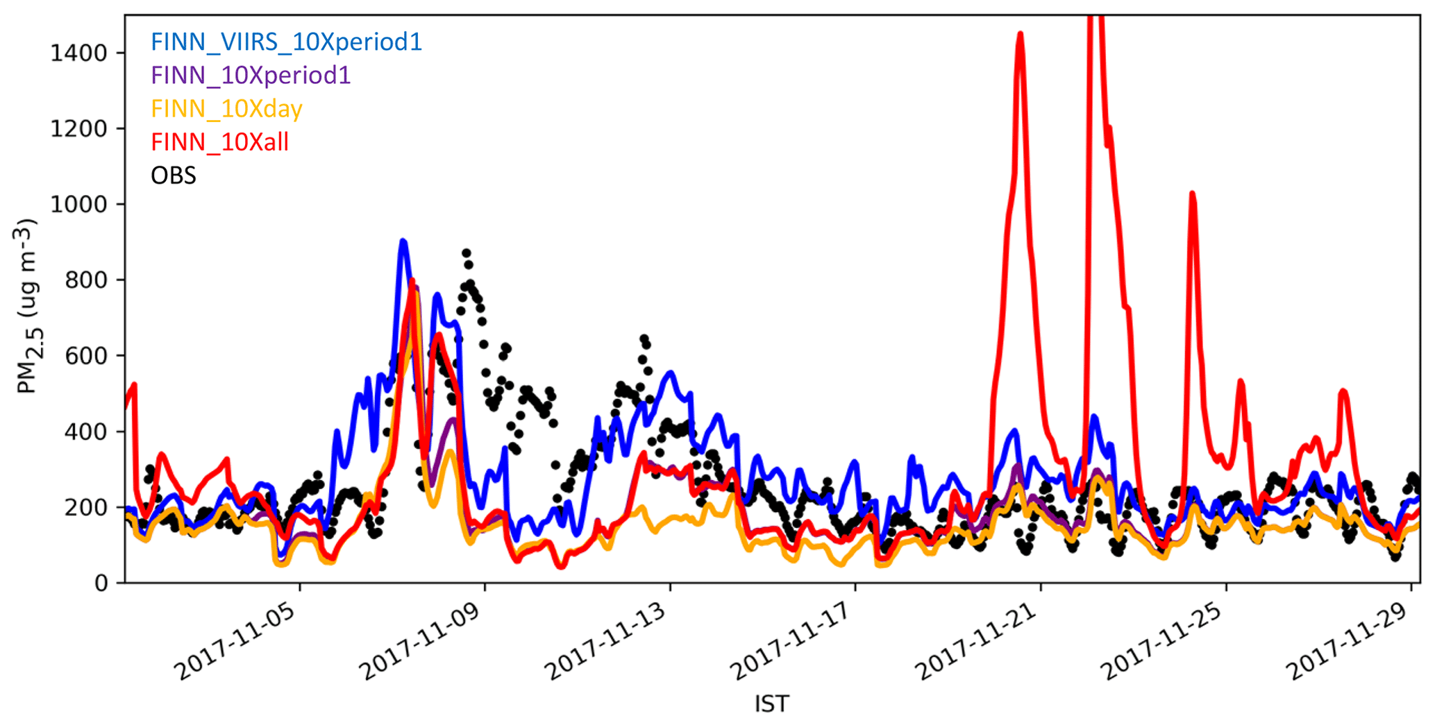
Figure 10Time series of model PM2.5 sensitivity to a 10-times increase in the FINN emission inventory for different periods: FINN_VIIRS_ 10Xperiod1, 3 to 17 November; FINN_10Xperiod1, 3 to 17 November; FINN_10xday, 5 November; and FINN_10Xall, all days. Black dots represent ground measurement data averaged over all CPCB stations in Delhi.
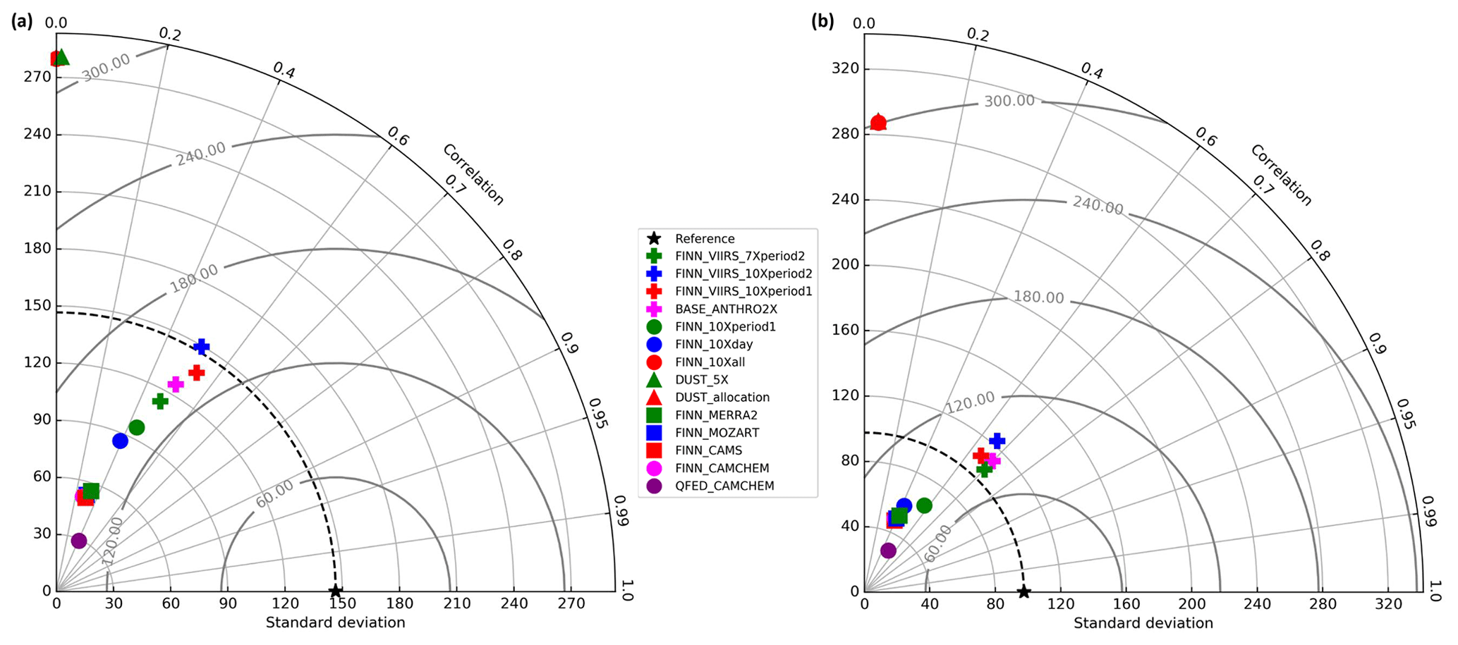
Figure 11Taylor diagram of hourly PM2.5 concentration based on different simulation scenarios for (a) all the days and (b) all the days except 8, 9, and 10 November. Plus signs denote experiments after incorporating VIIRS data into FINN; circles denote different experiments on the biomass burning emission inventory; triangles denote dust emission experiments; and squares denote chemical boundary condition experiments. Green colors show best performance in each experiment. The black star denotes standard deviation of all CPCB stations averaged in Delhi. The statistics plotted are standard deviation on the radial axis and Pearson's correlation coefficient (R) on the angular axis, and the gray lines indicate normalized centered RMSE (CRMSE).
Figure 12 shows vertical profiles of PM2.5 as a function of time at the US Embassy coordinates for variations using the FINN inventory and MERRA-2. Increasing the emissions in the FINN inventory significantly increased PM2.5 concentrations both vertically and temporally. Although the concentrations became closer to MERRA-2 data, the timing for the peak of the boundary layer on 6 November was different. By incorporating VIIRS data into FINN and adding more fire emissions, the boundary layer values peaked on 6 November earlier and look much more like MERRA-2 data. Figure 12 also shows more particles at altitudes above the boundary layer, which do not influence surface concentrations. Furthermore, it suggests the scaling factor for the base scenario could have been smaller than 7 if the aerosols had been in the boundary layer. This can be partly related to the plume rise module in WRF-Chem that may have emitted species at altitudes that were too high. Increasing emissions also indirectly influenced modeled air quality over Delhi. As our model configuration included feedbacks, absorbing aerosols in the atmosphere (products of fire emissions) decreased the surface solar radiation budget, changed the dynamics of the atmosphere, reduced the PBL height (PBLH), and increased aerosol concentrations. In other words, a higher PBLH leads to lower concentrations. For example, Murthy et al. (2020) found that PM2.5 concentration decreased by up to 14 µg m−3 for a 100 m increase in the PBLH. Figure 12 also shows the interactions between the PBLH and PM2.5 concentration at the location of the US Embassy. By increasing the FINN inventory by a factor of 7, the PBL height decreased by ∼50 % on 6 November, (compare FINN_VIIRS_7Xperiod2 and FINN_MERRA-2 panels in Fig. 12). However, a measured PBLH dataset can provide better insights. As a result, another study is required to compare modeled PBL heights to observed data (e.g., Nakoudi et al., 2019) and study the effects of different PBL parameterization modules on aerosol concentrations. Vertical profiles for other experiments using FINN can be found in the Supplement (Fig. S15).
We also performed two sets of experiments to understand if long-range-transported dust from the Middle East or in-boundary dust emissions impacted air quality in Delhi. Our sensitivity tests suggest that dust had a very low contribution to air quality in Delhi during November 2017. A detailed discussion on its impacts is presented in the Supplement.
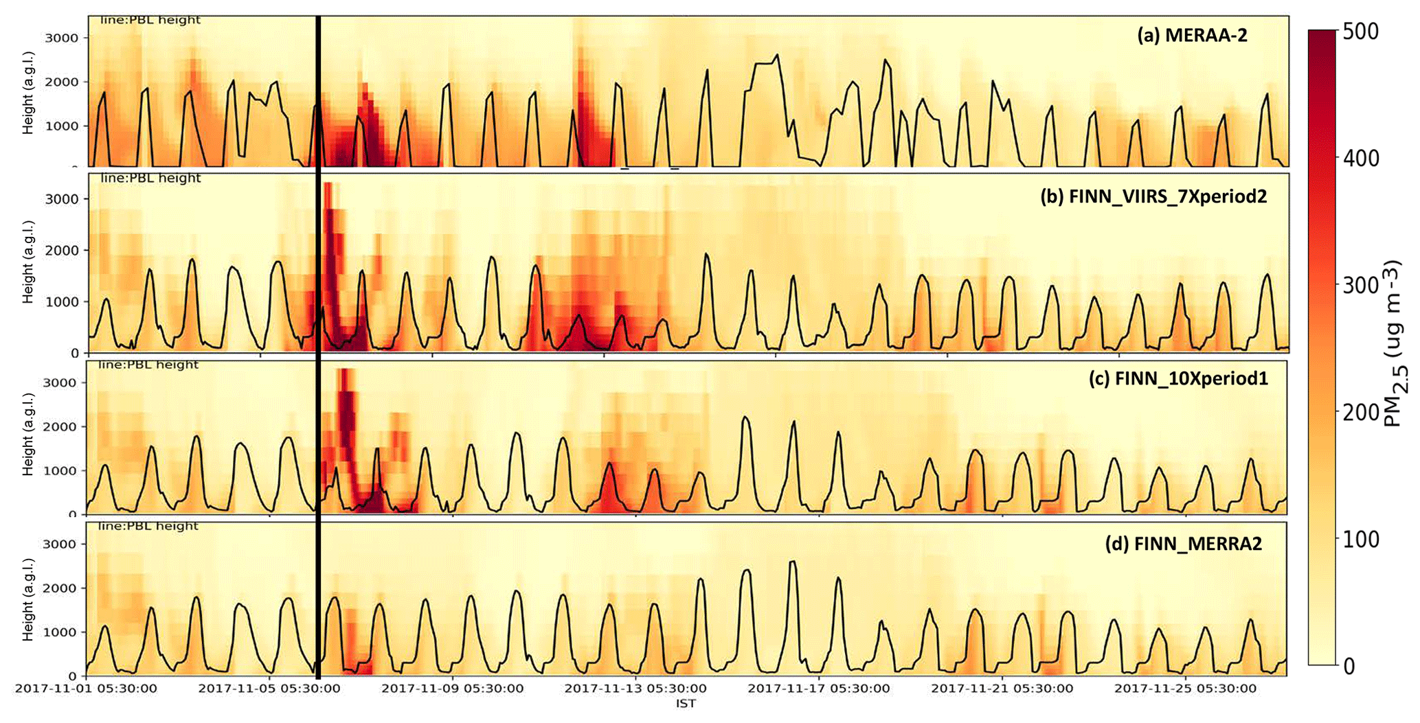
Figure 12Vertical cross section of PM2.5 sensitivity to major changes in the FINN emission inventory at US Embassy coordinates: (a) MERRA-2 data as true values, (b) FINN_VIIRS_7Xperiod2, (c) FINN_10Xperiod, and (d) FINN_MERRA2. Black lines represent planetary boundary layer height. Vertical black line crossing all panels shows boundary layer peak on 6 November for MERRA-2 and other experiments.
3.4 Aerosol composition in Delhi
We analyzed the modeled PM2.5 composition, both in concentrations and by mass fraction, at the location of the US Embassy in Delhi (Fig. S16). Secondary aerosols (secondary organic aerosols (SOAs) and secondary inorganic aerosols (SIAs) consisting of ammonium (NH4), nitrate (NO3), and sulfate (SO4)) comprised 57 % of the total averaged PM2.5 concentration while primary aerosols (BC, organic carbon (OC), and OIN) constituted the rest. Gani et al. (2019) measured PM1 in Delhi and reported 50 %–70 % for secondary aerosols, with PM1 constituting ∼85 % of PM2.5 concentration. SOAs, individually, comprise 27 % of the aerosol mass, while SIAs account for 30 % of the mass. Among inorganic species, NO3, NH4, and SO4 comprise 19 %, 7 %, and 4 %, respectively. Gani et al. (2019) reported the same ranked order but with different percentages. A major contribution of NO3 in winter is also reported in other studies (Pant et al., 2015). The BC fraction was 7 %, which is very close to the measured fraction of 6.4 % in wintertime PM1 (Gani et al., 2019). Pant et al. (2015) reported averaged OC and elemental carbon concentrations of 104.4 and 46.3 µg m−3, respectively, which is consistent with our ratio of 2.72. Comparing modeled BC1 data with available data for this period (Gani et al., 2019) shows an overall measured-to-modeled ratio of 1.22, which is consistent with the range other studies reported (Kumar et al., 2015b; Moorthy et al., 2013).
3.5 Ozone concentration analysis
Figure 13a shows the box-and-whisker plots for daytime (08:00–18:00 LT) ozone concentration for the base scenario and all of the CPCB stations in Delhi. Observed values ranged between 10 and 110 ppb, and the range between lower and upper quartiles was about 20 ppb, showing high ozone variability over Delhi. Moreover, observed values were higher during the extreme pollution episode. This indicates particles are not the only issue during PM pollution episodes in Delhi. The modeled median was in the range of observed values, especially on non-episode days. However, the model overestimated ozone concentrations on 7 November. Moreover, the range of observed ozone concentrations was wider than that of modeled values. In general, the model captured the trend fairly well with the correlation coefficient of 0.57 but was biased high with an NMB of 18 % for daytime hours throughout the whole of November. High-biased ozone concentration in Delhi is reported in other studies (Gupta and Mohan, 2015).
Figure 13b shows the daytime ozone concentration maps averaged over November 2017. Central regions of India show higher ozone concentrations compared to the northern IGP region. On the other hand, ozone concentration in urban regions were lower than in rural areas. This is due to lower ozone production in regions of higher NOx emissions in urban areas (Ghude et al., 2016; Karambelas et al., 2018). Averaged ozone concentration over the domain throughout November 2017 was 77 ppb using the base scenario. Ozone concentrations decreased by up to 27 ppb when using a scenario without any modifications to aerosol emissions (Fig. S17). Regardless, the averaged values are 9–17 ppb higher than the annual averaged concentration of 60 ppb in the year 2011 (Ghude et al., 2016). Overall, high measured and modeled ozone concentrations and positive correlation with PM2.5 are concerning and demand more studies. Moreover, recent observed values over Delhi indicated that, during the COVID-19 pandemic when many activities were suspended, PM2.5 concentration went down while the trend in and range of ozone concentration remained unchanged (Jain and Sharma, 2020).

Figure 13Daytime (08:00–18:00 LT) ozone modeling performance in the base scenario. (a) Box-and-whisker plots of observed (black) and modeled (purple) concentrations averaged over all CPCB stations in Delhi. (b) November 2017 daytime-averaged concentrations.
3.6 Study limitations
In this study, we used a simple framework to modify fire emissions with satellite data. Specifically, we used VIIRS data to fill FINN emissions, which are based on MODIS retrievals. We used VIIRS data as they had a higher resolution (375 m) for active fire points. Furthermore, we used linear regression to find the relation between VIIRS FRP and FINN emissions of available grid cells and applied that to FRP values in VIIRS to estimate the emissions. We acknowledge these are first estimates and the performance of this technique using MODIS data and more complicated statistical works needs to be studied further.
During this study, we did not focus on improving anthropogenic emissions over the region. However anthropogenic emissions are low in global emission inventories and need to be improved (Jat et al., 2020). Moreover, very low biased concentrations for some days and trajectory results suggest the existence of some other sources, primarily anthropogenic sources, upwind of Delhi that should be studied more.
Furthermore, geostationary satellites can significantly improve our technique as more retrievals could improve the accuracy. In this study, VIIRS or MODIS provided only one or two retrievals in 1 d for each point, while recently launched geostationary satellites, such as GEMS, would provide high-temporal-frequency data that could improve emission inventories.
The choice of the scaling factor for increasing fire emissions was arbitrary in this study. Due to scarcity of observation data, we were not able to apply complicated mathematical scaling techniques based on data assimilation to scale the fire emissions (Saide et al., 2015). A low number of observation data also limited our statistical assessments. Agricultural fire emissions are small and vary day to day, and atmospheric dynamics can significantly change their fate. We did not focus on the physics and dynamics of WRF-Chem as they were beyond the scope of this study. These are important limitations that readers have to keep in mind when assessing the results.
In this study, we used WRF-Chem to improve the air quality modeling during an extreme pollution episode in November 2017 in the IGP. Various modifications on chemical boundary conditions and biomass burning emissions were tested. Multiple datasets, including ground measurements of PM2.5, surface measurements and satellite AOD, and reanalysis models, were used to evaluate the model. In our best scenario, the CAM-chem and MERRA-2 global models provided gaseous and aerosol chemical boundary conditions, respectively. Moreover, active fire points in the VIIRS remote sensing instrument were used to fill the missing fire emission sources in FINN biomass burning emissions. Furthermore, the modified FINN emissions were scaled by a factor of 7 for an 8 d period to capture peak PM2.5 concentrations. Averaged for all CPCB stations in Delhi during all the days in November, the 24 h averaged NMB, NME, and R were −16.6 %, 27.6 %, and 0.48, respectively, satisfying suggested benchmark criteria (Emery et al., 2017). These metrics significantly improved when excluding 4 extremely polluted days between 7 and 10 November and all were within benchmark goals (Emery et al., 2017). Overall, we improved modeling results by combining different available datasets with each other.
The spatial performance of the model was also evaluated using VIIRS AOD. The model overestimated AOD over the domain with a monthly averaged value of 0.58 (±0.4), confirming other studies (Kulkarni et al., 2020). Specifically, the model captured high AODs over Delhi and Punjab, overestimated AODs over central India, and underestimated AODs over the eastern IGP. Our results indicate improving emissions, mostly anthropogenic emissions, in the eastern IGP can significantly improve the air quality predictions. Our modeling results revealed secondary aerosols comprised 57 % of total PM2.5 concentration during November, confirming measurement studies (Gani et al., 2019). Secondary organic aerosols individually comprised 27 % of the total aerosol mass, while secondary inorganics accounted for 30 % of the mass.
Back trajectories and vertical profiles were used to study the extreme-pollution-episode sources. Back trajectories showed a shift in trajectories from east to north on 7 November. As a result, agricultural fire emissions were transported from Punjab to Delhi. The trajectories remained on a northern path for 3 d and then shifted again to east. However, the model underestimated the concentrations on these days. Vertical profiles showed a lot of smoke above boundary layers. These results indicated either the plume rise in the model released the emissions too high or the model did not mix the smoke down fast enough. Social reasons can also add to high PM2.5 concentrations during extreme pollution episodes, as people prefer to use their personal vehicles more often.
We also evaluated how QFED and FINN biomass burning emission inventories affected PM2.5 concentration results over Delhi. QFED had worse statistics, which is mostly due to the inability of the inventory to capture the fire points over the domain. This can be attributed to both the technique and the resolution as QFED data have a ∼10 km resolution, whereas FINN data have a ∼1 km resolution, and other studies have shown FINN provides better data for India (Pan et al., 2020). We also found FINN underestimated fire emissions for some extremely high emission days and needed to be scaled. This can be mostly because satellite retrievals reported thick smoke as clouds and missed it, as shown in other studies (Dekker et al., 2019).
The base scenario was chosen after evaluating the results for various chemical boundary conditions, including the CAM-chem, MERRA-2, MOZART, and CAMS global models. We found long-range-transported dust from the Middle East did not affect Delhi's air quality during the extreme pollution episode. Moreover, we found MERRA-2 provided better aerosol products over India, although studies have shown it underestimates aerosols over India (Navinya et al., 2020). We also found in-domain dust emission sources at the border with Pakistan did not affect Delhi's air quality.
While the focus of the current study was on PM, we found high ozone concentration in northern India. Averaged daytime ozone concentration over the domain was 77 ppb for November 2017, using the base scenario. Although the model overestimated ozone concentrations in Delhi by an NMB of 18 %, it indicates ozone is a problem that needs to be considered.
In general, air quality in the IGP region is influenced by both local and regional sources. Although availability of new satellites such as GEMS, which covers some parts of India, can improve air quality predictions using data assimilation techniques, local emission inventories can vary day by day and significantly affect the modeling results. More works are required to quantify these impacts. Moreover, ozone concentrations showed a positive correlation with PM2.5 over the IGP. This suggests that control strategies should consider the regional co-benefits of PM2.5 and ozone perturbations simultaneously, which is the focus of our future work.
The WRF-Chem output results for aerosol species are available from Iowa Research Online at https://doi.org/10.25820/data.006126 (Roozitalab et al., 2020).
The supplement related to this article is available online at: https://doi.org/10.5194/acp-21-2837-2021-supplement.
BR and GRC designed the study; BR performed model simulations and analyzed the data with help from GRC and SKG provided measurements. BR and GRC wrote the paper with inputs from SKG.
The authors declare that they have no conflict of interest.
This article is part of the special issue “Regional assessment of air pollution and climate change over East and Southeast Asia: results from MICS-Asia Phase III”. It is not associated with a conference.
We acknowledge the use of data and imagery from LANCE FIRMS operated by NASA's Earth Science Data and Information System (ESDIS) with funding provided by NASA Headquarters. Moreover, this paper contains modified Copernicus Atmosphere Monitoring Service Information 2017, and neither the European Commission nor ECMWF is responsible for any use that may be made of the information it contains. The authors also thank Swagata Payra, Brent Holben, Sachchida Nand Tripathi, and their staff for establishing and maintaining the Jaipur and Kanpur AERONET station data used in this investigation. We thank Yannick Copin for his Python code for plotting Taylor diagrams. We also thank Pablo Saide for his comments on using the QFED emission inventory.
This research has been supported by the National Aeronautics and Space Administration (grant nos. NNX16AQ19G and 80NSSC19K094).
This paper was edited by Joshua Fu and reviewed by three anonymous referees.
Abdi-Oskouei, M., Carmichael, G., Christiansen, M., Ferrada, G., Roozitalab, B., Sobhani, N., Wade, K., Czarnetzki, A., Pierce, R., and Wagner, T.: Sensitivity of meteorological skill to selection of WRF-Chem physical parameterizations and impact on ozone prediction during the Lake Michigan Ozone Study (LMOS), J. Geophys. Res.-Atmos., 125, e2019JD031971, https://doi.org/10.1029/2019JD031971, 2020.
Adhikary, B., Carmichael, G. R., Tang, Y., Leung, L. R., Qian, Y., Schauer, J. J., Stone, E. A., Ramanathan, V., and Ramana, M. V.: Characterization of the seasonal cycle of south Asian aerosols: A regional-scale modeling analysis, J. Geophys. Res.-Atmos., 112, D22 https://doi.org/10.1029/2006JD008143, 2007.
Akagi, S. K., Yokelson, R. J., Wiedinmyer, C., Alvarado, M. J., Reid, J. S., Karl, T., Crounse, J. D., and Wennberg, P. O.: Emission factors for open and domestic biomass burning for use in atmospheric models, Atmos. Chem. Phys., 11, 4039–4072, https://doi.org/10.5194/acp-11-4039-2011, 2011.
Amann, M., Purohit, P., Bhanarkar, A. D., Bertok, I., Borken-Kleefeld, J., Cofala, J., Heyes, C., Kiesewetter, G., Klimont, Z., and Liu, J.: Managing future air quality in megacities: A case study for Delhi, Atmos. Environ., 161, 99–111, 2017.
Anenberg, S. C., Henze, D. K., Tinney, V., Kinney, P. L., Raich, W., Fann, N., Malley, C. S., Roman, H., Lamsal, L., and Duncan, B.: Estimates of the global burden of ambient PM2.5, ozone, and NO2 on asthma incidence and emergency room visits, Environ. Health Persp., 126, 107004, https://doi.org/10.1289/ehp3766, 2018.
Ashrafi, K., Motlagh, M. S., and Neyestani, S. E.: Dust storms modeling and their impacts on air quality and radiation budget over Iran using WRF-Chem, Air Qual. Atmos. Hlth., 10, 1059–1076, 2017.
Beig, G., Srinivas, R., Parkhi, N. S., Carmichael, G., Singh, S., Sahu, S. K., Rathod, A., and Maji, S.: Anatomy of the winter 2017 air quality emergency in Delhi, Sci. Total Environ., 681, 305–311, 2019.
Beig, G., Sahu, S. K., Singh, V., Tikle, S., Sobhana, S. B., Gargeva, P., Ramakrishna, K., Rathod, A., and Murthy, B.: Objective evaluation of stubble emission of North India and quantifying its impact on air quality of Delhi, Sci. Total Environ., 709, 136126, https://doi.org/10.1016/j.scitotenv.2019.136126, 2020.
Bosilovich, M. G., Lucchesi, R., and Suarez, M.: MERRA-2: File Specification. GMAO Office Note No. 9 (Version 1.1), 73 pp., available at: http://gmao.gsfc.nasa.gov/pubs/office_notes (last access: 24 February 2021), 2016.
Brioude, J., Arnold, D., Stohl, A., Cassiani, M., Morton, D., Seibert, P., Angevine, W., Evan, S., Dingwell, A., Fast, J. D., Easter, R. C., Pisso, I., Burkhart, J., and Wotawa, G.: The Lagrangian particle dispersion model FLEXPART-WRF version 3.1, Geosci. Model Dev., 6, 1889–1904, https://doi.org/10.5194/gmd-6-1889-2013, 2013.
Buchard, V., da Silva, A., Randles, C., Colarco, P., Ferrare, R., Hair, J., Hostetler, C., Tackett, J., and Winker, D.: Evaluation of the surface PM2.5 in version 1 of the NASA MERRA Aerosol Reanalysis over the United States, Atmos. Environ., 125, 100–111, 2016.
Chow, J. C., Lowenthal, D. H., Chen, L.-W. A., Wang, X., and Watson, J. G.: Mass reconstruction methods for PM2.5: a review, Air Qual. Atmos. Hlth., 8, 243–263, 2015.
Cohen, A. J., Brauer, M., Burnett, R., Anderson, H. R., Frostad, J., Estep, K., Balakrishnan, K., Brunekreef, B., Dandona, L., and Dandona, R.: Estimates and 25-year trends of the global burden of disease attributable to ambient air pollution: an analysis of data from the Global Burden of Diseases Study 2015, Lancet, 389, 1907–1918, 2017.
Conibear, L., Butt, E. W., Knote, C., Arnold, S. R., and Spracklen, D. V.: Residential energy use emissions dominate health impacts from exposure to ambient particulate matter in India, Nat. Commun., 9, 617, https://doi.org/10.1038/s41467-018-02986-7, 2018a.
Conibear, L., Butt, E. W., Knote, C., Spracklen, D. V., and Arnold, S. R.: Current and Future Disease Burden From Ambient Ozone Exposure in India, GeoHealth, 2, 334–355, 2018b.
Courant, R., Friedrichs, K., and Lewy, H.: Über die partiellen Differenzengleichungen der mathematischen Physik, Math. Ann., 100, 32–74, 1928.
Cusworth, D. H., Mickley, L. J., Sulprizio, M. P., Liu, T., Marlier, M. E., DeFries, R. S., Guttikunda, S. K., and Gupta, P.: Quantifying the influence of agricultural fires in northwest India on urban air pollution in Delhi, India, Environ. Res. Lett., 13, 044018, https://doi.org/10.1088/1748-9326/aab303, 2018.
David, L. M., Ravishankara, A., Kodros, J. K., Pierce, J. R., Venkataraman, C., and Sadavarte, P.: Premature mortality due to PM2.5 over India: Effect of atmospheric transport and anthropogenic emissions, GeoHealth, 3, 2–10, 2019.
Dekker, I. N., Houweling, S., Pandey, S., Krol, M., Röckmann, T., Borsdorff, T., Landgraf, J., and Aben, I.: What caused the extreme CO concentrations during the 2017 high-pollution episode in India?, Atmos. Chem. Phys., 19, 3433–3445, https://doi.org/10.5194/acp-19-3433-2019, 2019.
Emery, C., Tai, E., and Yarwood, G.: Enhanced meteorological modeling and performance evaluation for two Texas ozone episodes, Prepared for the Texas natural resource conservation commission, ENVIRON International Corp, Novato, CA, available at: https://www.tceq.texas.gov/assets/public/implementation/air/am/contracts/reports/mm/EnhancedMetModelingAndPerformanceEvaluation.pdf (last access: 24 February 2021), 2001.
Emery, C., Liu, Z., Russell, A. G., Odman, M. T., Yarwood, G., and Kumar, N.: Recommendations on statistics and benchmarks to assess photochemical model performance, J. Air Waste Manage., 67, 582–598, 2017.
Emmons, L. K., Walters, S., Hess, P. G., Lamarque, J.-F., Pfister, G. G., Fillmore, D., Granier, C., Guenther, A., Kinnison, D., Laepple, T., Orlando, J., Tie, X., Tyndall, G., Wiedinmyer, C., Baughcum, S. L., and Kloster, S.: Description and evaluation of the Model for Ozone and Related chemical Tracers, version 4 (MOZART-4), Geosci. Model Dev., 3, 43–67, https://doi.org/10.5194/gmd-3-43-2010, 2010.
Gani, S., Bhandari, S., Seraj, S., Wang, D. S., Patel, K., Soni, P., Arub, Z., Habib, G., Hildebrandt Ruiz, L., and Apte, J. S.: Submicron aerosol composition in the world's most polluted megacity: the Delhi Aerosol Supersite study, Atmos. Chem. Phys., 19, 6843–6859, https://doi.org/10.5194/acp-19-6843-2019, 2019.
GBD MAPS Working Group: Burden of Disease Attributable to Major Air Pollution Sources in India. Special Report 21, Health Effects Institute, Boston, MA, available at: https://www.healtheffects.org/system/files/GBD-MAPS-SpecRep21-India-revised_0.pdf (last access: 24 February 2021), 2018.
Gelaro, R., McCarty, W., Suárez, M. J., Todling, R., Molod, A., Takacs, L., Randles, C. A., Darmenov, A., Bosilovich, M. G., and Reichle, R.: The modern-era retrospective analysis for research and applications, version 2 (MERRA-2), J. Climate, 30, 5419–5454, 2017.
Ghude, S. D., Chate, D., Jena, C., Beig, G., Kumar, R., Barth, M., Pfister, G., Fadnavis, S., and Pithani, P.: Premature mortality in India due to PM2.5 and ozone exposure, Geophys. Res. Lett., 43, 4650–4658, 2016.
Ginoux, P., Chin, M., Tegen, I., Prospero, J. M., Holben, B., Dubovik, O., and Lin, S. J.: Sources and distributions of dust aerosols simulated with the GOCART model, J. Geophys. Res.-Atmos., 106, 20255–20273, 2001.
Grell, G. A., Peckham, S. E., Schmitz, R., McKeen, S. A., Frost, G., Skamarock, W. C., and Eder, B.: Fully coupled “online” chemistry within the WRF model, Atmos. Environ., 39, 6957–6975, 2005.
Guenther, A., Karl, T., Harley, P., Wiedinmyer, C., Palmer, P. I., and Geron, C.: Estimates of global terrestrial isoprene emissions using MEGAN (Model of Emissions of Gases and Aerosols from Nature), Atmos. Chem. Phys., 6, 3181–3210, https://doi.org/10.5194/acp-6-3181-2006, 2006.
Gupta, M. and Mohan, M.: Validation of WRF/Chem model and sensitivity of chemical mechanisms to ozone simulation over megacity Delhi, Atmos. Environ., 122, 220–229, 2015.
Guttikunda, S. K. and Calori, G.: A GIS based emissions inventory at 1 km × 1 km spatial resolution for air pollution analysis in Delhi, India, Atmos. Environ., 67, 101–111, 2013.
Guttikunda, S. K., Goel, R., and Pant, P.: Nature of air pollution, emission sources, and management in the Indian cities, Atmos. Environ., 95, 501–510, 2014.
He, L., Lin, A., Chen, X., Zhou, H., Zhou, Z., and He, P.: Assessment of MERRA-2 surface PM2.5 over the Yangtze river Basin: Ground-based verification, spatiotemporal distribution and meteorological dependence, Remote Sens., 11, 460, https://doi.org/10.3390/rs11040460, 2019.
Hodzic, A. and Jimenez, J. L.: Modeling anthropogenically controlled secondary organic aerosols in a megacity: a simplified framework for global and climate models, Geosci. Model Dev., 4, 901–917, https://doi.org/10.5194/gmd-4-901-2011, 2011.
Hodzic, A., Madronich, S., Kasibhatla, P. S., Tyndall, G., Aumont, B., Jimenez, J. L., Lee-Taylor, J., and Orlando, J.: Organic photolysis reactions in tropospheric aerosols: effect on secondary organic aerosol formation and lifetime, Atmos. Chem. Phys., 15, 9253–9269, https://doi.org/10.5194/acp-15-9253-2015, 2015.
Hsu, N., Lee, J., Sayer, A., Kim, W., Bettenhausen, C., and Tsay, S. C.: VIIRS Deep Blue aerosol products over land: Extending the EOS long-term aerosol data records, J. Geophys. Res.-Atmos., 124, 4026–4053, 2019.
Huijnen, V., Wooster, M. J., Kaiser, J. W., Gaveau, D. L., Flemming, J., Parrington, M., Inness, A., Murdiyarso, D., Main, B., and Van Weele, M.: Fire carbon emissions over maritime southeast Asia in 2015 largest since 1997, Sci. Rep.-UK, 6, 26886, https://doi.org/10.1038/srep26886, 2016.
Inness, A., Ades, M., Agustí-Panareda, A., Barré, J., Benedictow, A., Blechschmidt, A.-M., Dominguez, J. J., Engelen, R., Eskes, H., Flemming, J., Huijnen, V., Jones, L., Kipling, Z., Massart, S., Parrington, M., Peuch, V.-H., Razinger, M., Remy, S., Schulz, M., and Suttie, M.: The CAMS reanalysis of atmospheric composition, Atmos. Chem. Phys., 19, 3515–3556, https://doi.org/10.5194/acp-19-3515-2019, 2019.
Jain, S. and Sharma, T.: Social and Travel Lockdown Impact Considering Coronavirus Disease (COVID-19) on Air Quality in Megacities of India: Present Benefits, Future Challenges and Way Forward, Aerosol Air Qual. Res., 20, 1222–1236, 2020.
Janssens-Maenhout, G., Crippa, M., Guizzardi, D., Dentener, F., Muntean, M., Pouliot, G., Keating, T., Zhang, Q., Kurokawa, J., Wankmüller, R., Denier van der Gon, H., Kuenen, J. J. P., Klimont, Z., Frost, G., Darras, S., Koffi, B., and Li, M.: HTAP_v2.2: a mosaic of regional and global emission grid maps for 2008 and 2010 to study hemispheric transport of air pollution, Atmos. Chem. Phys., 15, 11411–11432, https://doi.org/10.5194/acp-15-11411-2015, 2015.
Jat, R., Gurjar, B. R., and Lowe, D.: Regional pollution loading in winter months over India using high resolution WRF-Chem simulation, Atmos. Res., 249, 105326, https://doi.org/10.1016/j.atmosres.2020.105326, 2020.
Jethva, H., Chand, D., Torres, O., Gupta, P., Lyapustin, A., and Patadia, F.: Agricultural burning and air quality over northern India: a synergistic analysis using NASA's A-train satellite data and ground measurements, Aerosol Air Qual. Res., 18, 1756–1773, 2018.
Karambelas, A., Holloway, T., Kinney, P. L., Fiore, A. M., DeFries, R., Kiesewetter, G., and Heyes, C.: Urban versus rural health impacts attributable to PM2.5 and O3 in northern India, Environ. Res. Lett., 13, 064010, https://doi.org/10.1088/1748-9326/aac24d, 2018.
Knote, C., Hodzic, A., Jimenez, J. L., Volkamer, R., Orlando, J. J., Baidar, S., Brioude, J., Fast, J., Gentner, D. R., Goldstein, A. H., Hayes, P. L., Knighton, W. B., Oetjen, H., Setyan, A., Stark, H., Thalman, R., Tyndall, G., Washenfelder, R., Waxman, E., and Zhang, Q.: Simulation of semi-explicit mechanisms of SOA formation from glyoxal in aerosol in a 3D model, Atmos. Chem. Phys., 14, 6213–6239, https://doi.org/10.5194/acp-14-6213-2014, 2014.
Koster, R. D., Darmenov, A. S., and da Silva, A. M.: The Quick Fire Emissions Dataset (QFED): Documentation of Versions 2.1, 2.2 and 2.4, vol. 38, Technical Report Series on Global Modeling and Data Assimilation, available at: https://ntrs.nasa.gov/citations/20180005253 (last access: 24 February 2021), 2015.
Kulkarni, S. H., Ghude, S. D., Jena, C., Karumuri, R. K., Sinha, B., Sinha, V., Kumar, R., Soni, V., and Khare, M.: How Much Does Large-Scale Crop Residue Burning Affect the Air Quality in Delhi?, Environ. Sci. Technol., 54, 4790–4799, 2020.
Kumar, R., Naja, M., Pfister, G. G., Barth, M. C., Wiedinmyer, C., and Brasseur, G. P.: Simulations over South Asia using the Weather Research and Forecasting model with Chemistry (WRF-Chem): chemistry evaluation and initial results, Geosci. Model Dev., 5, 619–648, https://doi.org/10.5194/gmd-5-619-2012, 2012.
Kumar, R., Barth, M. C., Madronich, S., Naja, M., Carmichael, G. R., Pfister, G. G., Knote, C., Brasseur, G. P., Ojha, N., and Sarangi, T.: Effects of dust aerosols on tropospheric chemistry during a typical pre-monsoon season dust storm in northern India, Atmos. Chem. Phys., 14, 6813–6834, https://doi.org/10.5194/acp-14-6813-2014, 2014a.
Kumar, R., Barth, M. C., Pfister, G. G., Naja, M., and Brasseur, G. P.: WRF-Chem simulations of a typical pre-monsoon dust storm in northern India: influences on aerosol optical properties and radiation budget, Atmos. Chem. Phys., 14, 2431–2446, https://doi.org/10.5194/acp-14-2431-2014, 2014b.
Kumar, R., Barth, M. C., Nair, V. S., Pfister, G. G., Suresh Babu, S., Satheesh, S. K., Krishna Moorthy, K., Carmichael, G. R., Lu, Z., and Streets, D. G.: Sources of black carbon aerosols in South Asia and surrounding regions during the Integrated Campaign for Aerosols, Gases and Radiation Budget (ICARB), Atmos. Chem. Phys., 15, 5415–5428, https://doi.org/10.5194/acp-15-5415-2015, 2015a.
Kumar, R., Barth, M., Pfister, G., Nair, V., Ghude, S. D., and Ojha, N.: What controls the seasonal cycle of black carbon aerosols in India?, J. Geophys. Res.-Atmos., 120, 7788–7812, 2015b.
Kumar, R., Ghude, S. D., Biswas, M., Jena, C., Alessandrini, S., Debnath, S., Kulkarni, S., Sperati, S., Soni, V. K., and Nanjundiah, R. S.: Enhancing Accuracy of Air Quality and Temperature Forecasts During Paddy Crop Residue Burning Season in Delhi Via Chemical Data Assimilation, J. Geophys. Res.-Atmos., 125, e2020JD033019, https://doi.org/10.1029/2020JD033019, 2020.
Liu, T., Marlier, M. E., DeFries, R. S., Westervelt, D. M., Xia, K. R., Fiore, A. M., Mickley, L. J., Cusworth, D. H., and Milly, G.: Seasonal impact of regional outdoor biomass burning on air pollution in three Indian cities: Delhi, Bengaluru, and Pune, Atmos. Environ., 172, 83–92, 2018.
Marrapu, P., Cheng, Y., Beig, G., Sahu, S., Srinivas, R., and Carmichael, G. R.: Air quality in Delhi during the Commonwealth Games, Atmos. Chem. Phys., 14, 10619–10630, https://doi.org/10.5194/acp-14-10619-2014, 2014.
MoEF&CC: Nation Clean Air Programme (NCAP), Ministry of Environment, Forest & Climate Change, India, 122 pp., 2019.
Moorthy, K. K., Beegum, S. N., Srivastava, N., Satheesh, S., Chin, M., Blond, N., Babu, S. S., and Singh, S.: Performance evaluation of chemistry transport models over India, Atmos. Environ., 71, 210–225, 2013.
Morrison, H., Curry, J., and Khvorostyanov, V.: A new double-moment microphysics parameterization for application in cloud and climate models, Part I: Description, J. Atmos. Sci., 62, 1665–1677, 2005.
Murthy, B., Latha, R., Tiwari, A., Rathod, A., Singh, S., and Beig, G.: Impact of mixing layer height on air quality in winter, J. Atmos. Sol.-Terr. Phy., 197, 105157, https://doi.org/10.1016/j.jastp.2019.105157, 2020.
Nakanishi, M. and Niino, H.: Development of an improved turbulence closure model for the atmospheric boundary layer, J. Meteorol. Soc. Jpn., 87, 895–912, 2009.
Nakoudi, K., Giannakaki, E., Dandou, A., Tombrou, M., and Komppula, M.: Planetary boundary layer height by means of lidar and numerical simulations over New Delhi, India, Atmos. Meas. Tech., 12, 2595–2610, https://doi.org/10.5194/amt-12-2595-2019, 2019.
Navinya, C. D., Vinoj, V., and Pandey, S. K.: Evaluation of PM2.5 Surface Concentrations Simulated by NASA's MERRA Version 2 Aerosol Reanalysis over India and its Relation to the Air Quality Index, Aerosol Air Qual. Res., 20, 1329–1339, 2020.
Pan, X., Ichoku, C., Chin, M., Bian, H., Darmenov, A., Colarco, P., Ellison, L., Kucsera, T., da Silva, A. M., Wang, J., Oda, T., and Cui, G.: Six global biomass burning emission datasets: intercomparison and application in one global aerosol model, Atmos. Chem. Phys., 20, 969–994, https://doi.org/10.5194/acp-20-969-2020, 2020.
Pant, P., Shukla, A., Kohl, S. D., Chow, J. C., Watson, J. G., and Harrison, R. M.: Characterization of ambient PM2.5 at a pollution hotspot in New Delhi, India and inference of sources, Atmos. Environ., 109, 178–189, 2015.
Provençal, S., Buchard, V., da Silva, A. M., Leduc, R., Barrette, N., Elhacham, E., and Wang, S.-H.: Evaluation of PM2.5 surface concentration simulated by Version 1 of the NASA's MERRA Aerosol Reanalysis over Israel and Taiwan, Aerosol Air Qual. Res., 17, 253–261, https://doi.org/10.4209/aaqr.2016.04.0145, 2017.
Rajak, R. and Chattopadhyay, A.: Short and long-term exposure to ambient air pollution and impact on health in India: a systematic review, Int. J. Environ. Heal. R., 30, 593–617, https://doi.org/10.1080/09603123.2019.1612042, 2020.
Ramanathan, V. and Carmichael, G.: Global and regional climate changes due to black carbon, Nat. Geosci., 1, 221–227, https://doi.org/10.1038/ngeo156, 2008.
Randles, C., da Silva, A. M., Buchard, V., Colarco, P., Darmenov, A., Govindaraju, R., Smirnov, A., Holben, B., Ferrare, R., and Hair, J.: The MERRA-2 aerosol reanalysis, 1980 onward, Part I: System description and data assimilation evaluation, J. Climate, 30, 6823–6850, 2017.
Saide, P. E., Peterson, D. A., da Silva, A. M., Anderson, B., Ziemba, L. D., Diskin, G., Sachse, G., Hair, J., Butler, C., and Fenn, M.: Revealing important nocturnal and day-to-day variations in fire smoke emissions through a multiplatform inversion, Geophys. Res. Lett., 42, 3609–3618, 2015.
Saikawa, E., Trail, M., Zhong, M., Wu, Q., Young, C. L., Janssens-Maenhout, G., Klimont, Z., Wagner, F., Kurokawa, J.-I., and Nagpure, A. S.: Uncertainties in emissions estimates of greenhouse gases and air pollutants in India and their impacts on regional air quality, Environ. Res. Lett., 12, 065002, https://doi.org/10.1088/1748-9326/aa6cb4, 2017.
Schroeder, W., Oliva, P., Giglio, L., and Csiszar, I. A.: The New VIIRS 375 m active fire detection data product: Algorithm description and initial assessment, Remote Sens. Environ., 143, 85–96, 2014.
Sharma, A., Ojha, N., Pozzer, A., Mar, K. A., Beig, G., Lelieveld, J., and Gunthe, S. S.: WRF-Chem simulated surface ozone over south Asia during the pre-monsoon: effects of emission inventories and chemical mechanisms, Atmos. Chem. Phys., 17, 14393–14413, https://doi.org/10.5194/acp-17-14393-2017, 2017.
Sitch, S., Cox, P., Collins, W., and Huntingford, C.: Indirect radiative forcing of climate change through ozone effects on the land-carbon sink, Nature, 448, 791–794, 2007.
Song, Z., Fu, D., Zhang, X., Wu, Y., Xia, X., He, J., Han, X., Zhang, R., and Che, H.: Diurnal and seasonal variability of PM2.5 and AOD in North China plain: Comparison of MERRA-2 products and ground measurements, Atmos. Environ., 191, 70–78, 2018.
Turpin, B. J. and Lim, H.-J.: Species contributions to PM2.5 mass concentrations: Revisiting common assumptions for estimating organic mass, Aerosol. Sci. Tech., 35, 602–610, 2001.
US Environmental Protection Agency: Integrated science assessment for ozone and related photochemical oxidants, EPA 600/R-10/076F, available at: https://www.epa.gov/isa/integrated-science-assessment-isa-ozone-and-related-photochemical-oxidants (last access: 24 February 2021), 2013.
Venkataraman, C., Brauer, M., Tibrewal, K., Sadavarte, P., Ma, Q., Cohen, A., Chaliyakunnel, S., Frostad, J., Klimont, Z., Martin, R. V., Millet, D. B., Philip, S., Walker, K., and Wang, S.: Source influence on emission pathways and ambient PM2.5 pollution over India (2015–2050), Atmos. Chem. Phys., 18, 8017–8039, https://doi.org/10.5194/acp-18-8017-2018, 2018.
Vijayakumar, K., Safai, P., Devara, P., Rao, S. V. B., and Jayasankar, C.: Effects of agriculture crop residue burning on aerosol properties and long-range transport over northern India: a study using satellite data and model simulations, Atmos. Res., 178, 155–163, 2016.
Wang, W., Bruyere, C., Duda, M., Dudhia, J., Gill, D., Kavulich, M., Keene, K., Lin, H., Michalakes, J., and Rizvi, S.: User's Guides for the Advanced Research WRF (ARW) Modeling System, version 3, available at: https://www2.mmm.ucar.edu/wrf/users/docs/user_guide_V3/contents.html (last access: 24 February 2021), 2018.
WHO: WHO Air quality guidelines for particulate matter, ozone, nitrogen dioxide and sulfur dioxide: global update 2005: summary of risk assessment, World Health Organization, Geneva, Switzerland, available at: https://apps.who.int/iris/handle/10665/69477 (last access: 24 February 2021), 2006.
WHO: WHO global urban ambient air pollution database (update 2016), Geneva, Diunduh, WHO, Switzerland, available at: https://www.who.int/airpollution/data/cities-2016/en/ (last access: 24 February 2021), 2016.
Wiedinmyer, C., Akagi, S. K., Yokelson, R. J., Emmons, L. K., Al-Saadi, J. A., Orlando, J. J., and Soja, A. J.: The Fire INventory from NCAR (FINN): a high resolution global model to estimate the emissions from open burning, Geosci. Model Dev., 4, 625–641, https://doi.org/10.5194/gmd-4-625-2011, 2011.
World-Bank: India: Systematic Countary Diagnostic, Realizing the promise of prosperity, World Bank 126284-IN, available at: http://documents.worldbank.org/curated/en/629571528745663 168/India-Systematic-country-diagnostic-realizing-the-promise-of-prosperity (last access: 24 February 2021), 2018.
Xiu, D.: Numerical methods for stochastic computations: a spectral method approach, Princeton, New Jersey, USA, 127 pp., https://doi.org/10.2307/j.ctv7h0skv, 2010.
Zaveri, R. A., Easter, R. C., Fast, J. D., and Peters, L. K.: Model for simulating aerosol interactions and chemistry (MOSAIC), J. Geophys. Res.-Atmos., 113, D13204, https://doi.org/10.1029/2007JD008782, 2008.
Zhao, C., Liu, X., Leung, L. R., Johnson, B., McFarlane, S. A., Gustafson Jr., W. I., Fast, J. D., and Easter, R.: The spatial distribution of mineral dust and its shortwave radiative forcing over North Africa: modeling sensitivities to dust emissions and aerosol size treatments, Atmos. Chem. Phys., 10, 8821–8838, https://doi.org/10.5194/acp-10-8821-2010, 2010.