the Creative Commons Attribution 4.0 License.
the Creative Commons Attribution 4.0 License.
 | 22 Dec 2021
The role of anthropogenic aerosols in the anomalous cooling from 1960 to 1990 in the CMIP6 Earth system models
Jie Zhang
Kalli Furtado
Steven T. Turnock
Jane P. Mulcahy
Laura J. Wilcox
Ben B. Booth
David Sexton
Tongwen Wu
Fang Zhang
Qianxia Liu
The Earth system models (ESMs) that participated in the sixth Coupled Model Intercomparison Project (CMIP6) tend to simulate excessive cooling in surface air temperature (TAS) between 1960 and 1990. The anomalous cooling is pronounced over the Northern Hemisphere (NH) midlatitudes, coinciding with the rapid growth of anthropogenic sulfur dioxide (SO2) emissions, the primary precursor of atmospheric sulfate aerosols. Structural uncertainties between ESMs have a larger impact on the anomalous cooling than internal variability. Historical simulations with and without anthropogenic aerosol emissions indicate that the anomalous cooling in the ESMs is attributed to the higher aerosol burden in these models. The aerosol forcing sensitivity, estimated as the outgoing shortwave radiation (OSR) response to aerosol concentration changes, cannot well explain the diversity of pothole cooling (PHC) biases in the ESMs. The relative contributions to aerosol forcing sensitivity from aerosol–radiation interactions (ARIs) and aerosol–cloud interactions (ACIs) can be estimated from CMIP6 simulations. We show that even when the aerosol forcing sensitivity is similar between ESMs, the relative contributions of ARI and ACI may be substantially different. The ACI accounts for between 64 % and 87 % of the aerosol forcing sensitivity in the models and is the main source of the aerosol forcing sensitivity differences between the ESMs. The ACI can be further decomposed into a cloud-amount term (which depends linearly on cloud fraction) and a cloud-albedo term (which is independent of cloud fraction, to the first order), with the cloud-amount term accounting for most of the inter-model differences.
- Article
(8691 KB) - Full-text XML
- Companion paper
- BibTeX
- EndNote


Surface air temperature (TAS) variation is an essential indicator of climate change, and reproducing the evolution of historical TAS is a crucial criterion for model evaluation. However, the historical TAS anomaly simulated by the models in the sixth Coupled Model Intercomparison Project (CMIP6) is on average colder than that observed in the mid-20th century, whereas the CMIP5 models tracked the instrumental TAS variation quite well (Flynn and Mauritsen, 2020). This is surprising because the transient climate response in CMIP6 models is generally higher than in CMIP5 models (e.g., Flynn and Mauritsen, 2020; Meehl et al., 2020).
As a result of anthropogenic emissions, atmospheric aerosol concentrations increased along with rising greenhouse gases, but with greater decadal variability. Aerosols are generally not evenly distributed around the planet as greenhouse gases, and they have relatively short lifetimes of the order of a week. Aerosols increased rapidly in the mid-20th century, predominantly due to US and European emissions. The rate of change of global aerosol emissions slowed down in the late 20th century (Hoesly et al., 2018), and the trend of global emission has been negative since the mid-2000s (Klimont et al., 2013). There has also been a shift in emission source regions. European and US emissions have declined following the introduction of clean air legislation since the 1980s, while Asian emissions have risen due to economic development. East Asian emissions clearly increased from 2000 to 2005, followed by a decrease with large uncertainties (Aas et al., 2019). The decade-long emission reduction since 2006 over East China is not well represented by the CMIP6 emission (Wang et al., 2021).
Although greenhouse warming was concluded to be the dominant forcing for long-term changes (e.g., Weart, 2008; Bindoff et al., 2013), multidecadal variability in TAS and the reduced rate of warming in the mid-20th century in particular have been attributed to aerosol forcing (e.g., Wilcox et al., 2013). Ramanathan and Feng (2009) noted that the aerosol cooling effect might have masked as much as 47 % of the global warming by greenhouse gases in the year 2005, with an uncertainty range of 20 %–80 %. The aerosol cooling effect is mainly attributed to the ability of sulfate particles to reflect incoming solar radiation and modify the microphysical properties of clouds (e.g., Charlson et al., 1990; Mitchell et al., 1995; Lohmann and Feichter, 2005). The increase in anthropogenic aerosols was also responsible for weakening the hydrological cycle between the 1950s and the 1980s (Wu et al., 2013).
Previous work has suggested that the anomalous mid-20th century cooling in the CMIP6 models is the result of excessive aerosol forcing. Flynn and Mauritsen (2020) suggested that aerosol cooling is too strong in many CMIP6 models because there is no apparent relationship between the warming trends simulated by models and their transient climate responses (TCRs) before the 1970s. Dittus et al. (2020) found that historical simulations can better capture the observed historical record by reducing the aerosol emissions in HadGEM3-GC3.1, demonstrating an overly strong aerosol cooling effect. In this study we characterize the mid-20th century excessive cooling in CMIP6 Earth system models (ESMs). In order to quantify the role of aerosol processes in this anomalous cooling, historical experiments with and without anthropogenic aerosol emissions are employed. The remainder of the paper is organized as follows. Section 2 introduces the models, data, and a quantitative method to separate the aerosol forcing components. The major features of anomalous cooling in CMIP6 ESMs are examined in Sect. 3. Section 4 investigates the possible reasons for the anomalous cooling. The relative importance of aerosol–radiation interactions and aerosol–cloud interactions in each ESM is quantified and discussed in Sect. 5. Conclusion is given in Sect. 6.
Table 1Information of the ESMs with an interactive chemistry and aerosol scheme, as well as the corresponding lower-complexity models.

2.1 CMIP6 ESMs
CMIP6 includes an unprecedented number of models with representations of aerosol–cloud interactions. Many also have interactive tropospheric chemistry and aerosol schemes. Six such ESMs are employed in this study: BCC-ESM1 (Wu et al., 2020; Zhang et al., 2021), EC-Earth-AerChem (van Noije et al., 2021), GFDL-ESM4 (Dunne et al., 2020), MPI-ESM-1-2-HAM (Neubauer et al., 2019), NorESM2-LM (Seland et al., 2020), and UKESM1-0-LL (Sellar et al., 2019). The surface air temperature simulated in corresponding models with lower-complexity is also examined: BCC-CSM2-MR (Wu et al., 2019b), EC-Earth3 (Döscher et al., 2021), and MPI-ESM1-2-LR (Mauritsen et al., 2019) with prescribed tropospheric chemistry and aerosol; GFDL-CM4 (Held et al., 2019), NorCPM1 (Bethke et al., 2019), and HadGEM3-GC31-LL (Williams et al., 2017) with a prescribed tropospheric chemistry and interactive aerosol scheme. BCC-CSM2-MR, EC-Earth3, and MPI-ESM1-2-LR prescribe the anthropogenic aerosol forcings using the MACv2-SP parameterization (Stevens et al., 2017). MACv2-SP approximates the observationally constrained spatial distributions of the monthly mean anthropogenic aerosol optical properties and an associated Twomey effect. A brief summary of the ESMs and the lower-complexity models is introduced in Table 1.
2.2 Data
The CMIP6 historical experiment and hist-piAer experiment are employed. The historical experiment is forced by time-evolving, externally imposed natural and anthropogenic forcings, such as solar variability, volcanic aerosols, greenhouse gases, and aerosol emissions (Eyring et al., 2016). The hist-piAer experiment is designed by the CMIP6-endorsed Aerosol Chemistry Model Intercomparison Project (AerChemMIP; Collins et al., 2017). It is run in parallel with the historical experiment but fixes aerosol and aerosol precursor emissions to pre-industrial conditions. Therefore, the differences between these two experiments are attributable to anthropogenic aerosol emissions. The design of the hist-piAer simulation means that it can also capture any non-linearities resulting from greenhouse-gas-driven changes in clouds. This is in contrast to the hist-aer simulations available from the Detection and Attribution Model Intercomparison Project (DAMIP; Gillett et al., 2016), which resembles the historical simulations but is only forced by transient changes in aerosol.
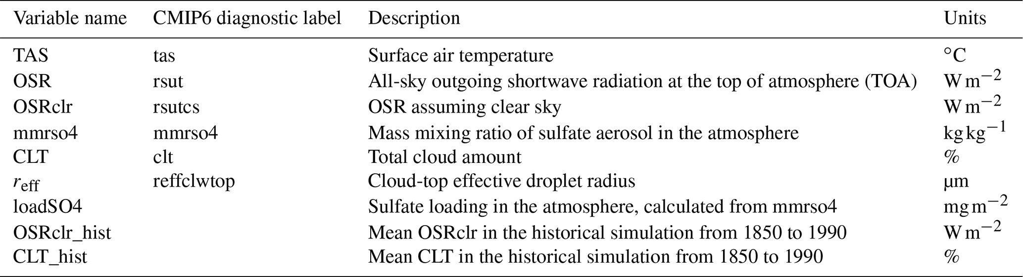
The monthly outputs from historical and hist-piAer simulations for ESMs are used, including TAS, all-sky outgoing shortwave radiation at the top of atmosphere (OSR), OSR assuming clear sky (OSRclr), mass mixing ratio of sulfate aerosol in the atmosphere (mmrso4), total cloud amount (CLT), and cloud-top effective droplet radius (reff). These variables are summarized in Table 2. The corresponding lower-complexity models have conducted the historical but not the hist-piAer simulations, and only the monthly TAS output from the historical simulations is used. Therefore, we focus on the ESMs when identifying the main aerosol processes contributing to the anomalous cooling.
The verification data used in this study is HadCRUT5, the monthly 5∘ latitude by 5∘ longitude gridded surface temperature (Morice et al., 2021), a blend of the Met Office Hadley Centre SST data set HadSST4 (Kennedy et al., 2019) and the land surface air temperature CRUTEM5 (Osborn et al., 2021).
2.3 Method
By comparing the TAS anomalies in ESMs and the lower-complexity models with HadCRUT5, our study found that TAS anomalies from 1960 to 1990 relative to 1850–1900 in ESMs and most of the lower-complexity models are on average much lower than observed, resembling a pothole shape. The magnitude of this anomalous cooling, i.e., the pothole cooling (PHC), is quantified as the near-global mean (60∘ S to 65∘ N) difference in the TAS anomaly between models and HadCRUT5 from 1960 to 1990. The variations over the polar regions (north of 65∘ N and south of 60∘ S) are not considered due to the lack of long-term reliable observations (Wu et al., 2019a).
The aerosol cooling is dominated by the contribution of sulfate aerosol as estimated by models and observations (Myhre et al., 2013; Smith et al., 2020). We use the evolution of sulfate loading (loadSO4) through the historic simulation as a proxy for total aerosol concentration changes to link estimates of the impact of aerosol forcing. Whilst the overall impact of aerosol forcing will also depend on other aerosol species, we adopt this approach because the sulfates dominate estimates of aerosol forcing during this period and other aerosols species can be assumed (as a first-order approximation) to have covaried with the SO2 emissions during this period as presented by the Community Emissions Data System (CEDS) inventory adopted by CMIP6 models (Hoesly et al., 2018). As such when we present estimates of the aerosol impact/loadSO4 we are presenting the impact of all aerosol species (including absorbing aerosols such as black carbon) as they covary with the sulfate concentrations during the historic period. The motivation for presenting it in this way is we can separate differences in ESM responses to changes in aerosol amount from the differences in aerosol amount (represented by loadSO4) simulated by the ESMs.
We can estimate the impact of anthropogenic aerosol by using the difference in OSR between the historical and hist-piAer simulations, ΔOSR. ΔOSR of course involves any differences in natural variability and planetary albedo between the two simulations, including clear-sky albedo changes and any adjustments in the microphysical or macroscopic properties of clouds. The sensitivity of the OSR response to aerosol changes, i.e., the aerosol forcing sensitivity, can be measured by the linear fit slope between the annual mean globally averaged OSR differences and loadSO4 differences between the historical and hist-piAer simulations:
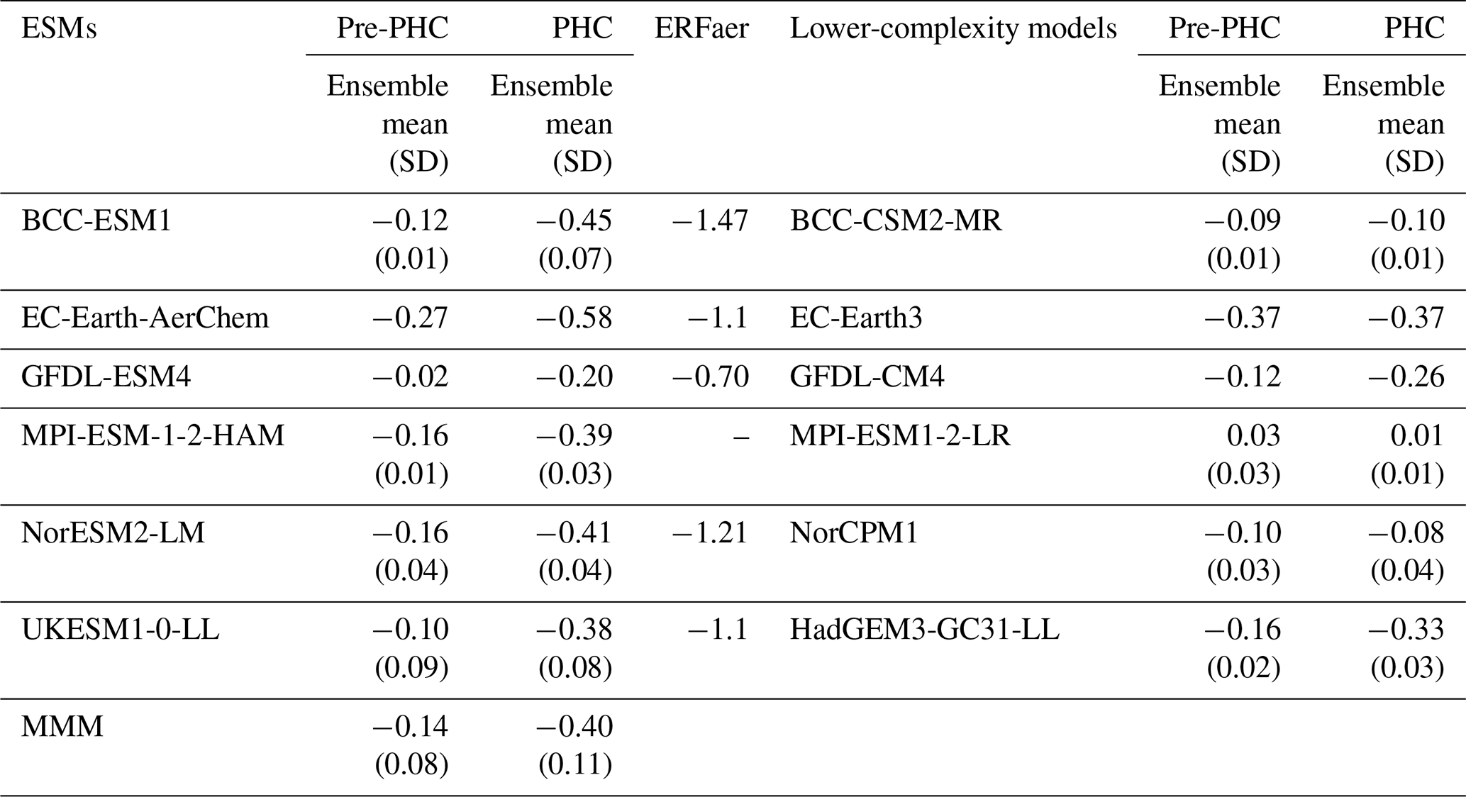
Table 3Biases in near-global averaged TAS anomalies relative to 1850–1900 from the ensemble mean and standard deviation (SD) for each ESM and the corresponding lower-complexity model in the pre-PHC (1929–1959) and the PHC period. Units: ∘C. Biases are relative to the HadCRUT5. The multi-model mean (MMM) and the SD of the ESMs are shown in the bottom row. The aerosol effective forcing (ERFaer) is also shown for each ESM except for MPI-ESM-1-2-HAM. ERFaer result for MPI-ESM-1-2-HAM are not available.
In this study, we diagnose the OSR differences from historical simulations that also capture the temperature response. As such the OSR differences do not represent a measure of only the aerosol forcing impact but combine OSR differences arising from both the aerosol forcing and the temperature response to this forcing, which we refer to in this paper as the aerosol forcing sensitivity. It presents a measure of the importance of aerosol changes in simulated temperature changes that can be easily calculated for existing transient simulations. The aerosol forcing sensitivity is different from the commonly used aerosol effective radiative forcing (ERFaer), which is the change in net TOA downward radiative flux after allowing adjustments in the atmosphere, but with sea surface temperatures and sea ice cover fixed at climatological values. The ERFaer for each ESM except MPI-ESM-1-2-HAM is listed in Table 3. The ERFaer is not correlated with the aerosol forcing sensitivity.
The aerosol forcing sensitivity can be further partitioned into a contribution from aerosol–radiation interactions (ARIs) and aerosol–cloud interactions (ACIs). ARI and ACI can be readily estimated from the CMIP6 output because annual mean cloud amount (CLT), OSR, and the OSR assuming only clear sky (OSRclr) are available for all the CMIP6 ESMs. For each model, the clear-sky part OSR, OSRclr_p, can be estimated as . The aerosol forcing sensitivity in the clear-sky part can therefore be estimated as
where CLT_hist and OSRclr_hist are the mean CLT and OSRclr in the historical experiment. The aerosol forcing sensitivity in the cloudy part are relative to the cloud-amount response to aerosol loading and cloud radiative effect changes and can be estimated as
Therefore, the aerosol forcing sensitivity can be decomposed as
where M, N, and A are empirically determined parameters. The parameter M is the slope of a linear fit of ΔOSRclr to ΔloadSO4 and therefore measures the strength of the aerosol–radiation interactions in each model. The first term on the right-hand side of Eq. (4), , can therefore be identified with ARI. The parameter A is the slope of a linear fit of ΔOSRcld to ΔCLT and therefore measures the correlation of the shortwave radiation reflected by clouds with changes in cloud amount. That is, the parameter A represents the baseline cloud albedo which is sensitive to the cloud parameterizations via cloud droplet number concentration (CDNC), cloud-droplet effective radius, and other factors. The parameter N is the slope of a linear fit of ΔCLT to ΔloadSO4 and therefore measures the sensitivity of cloud amount to aerosols. Note that changes in cloud amount by definition also affect the fraction of clear sky; hence, increases in OSRcld due to increases in CLT (i.e., A⋅N) can be partly offset by changes in area of clear sky containing aerosols (). The second term on the right-hand side of Eq. (4), , can therefore contribute to the ACI. Specifically, it is the part of ACI that is linearly proportional to changes to cloud fraction, which we will refer to in this paper as the cloud-amount term. It is therefore sensitive to any aerosol-induced cloud fraction changes (Lohmann and Feichter, 2005), including any slow adjustments in clouds due to feedbacks within the Earth system.
In addition to depending on ΔCLT, ACI is also influenced by any changes in cloud albedo that might occur independently of cloud-amount changes. Such adjustments would include increases in cloud droplet number concentration and increases in simulated cloud-droplet effective radius without accompanying changes in cloud cover. Changes purely in the brightness of clouds, without changes in macroscopic properties of clouds, are difficult to identify from the CMIP6 output because all the bulk properties of clouds co-vary over the course of the projections. However, subtracting ARI and the cloud-amount term from the aerosol forcing sensitivity gives a residual that is, by definition, linearly independent of cloud fraction differences (since by construction these have been regressed out). This residual can then be interpreted as due to differences in the albedo of clouds between the historical and hist-piAer and will be called the “cloud-albedo term”. Note that this method of calculation implies that purely albedo effects cannot be distinguished from general residual terms that result from the linear approximation made.
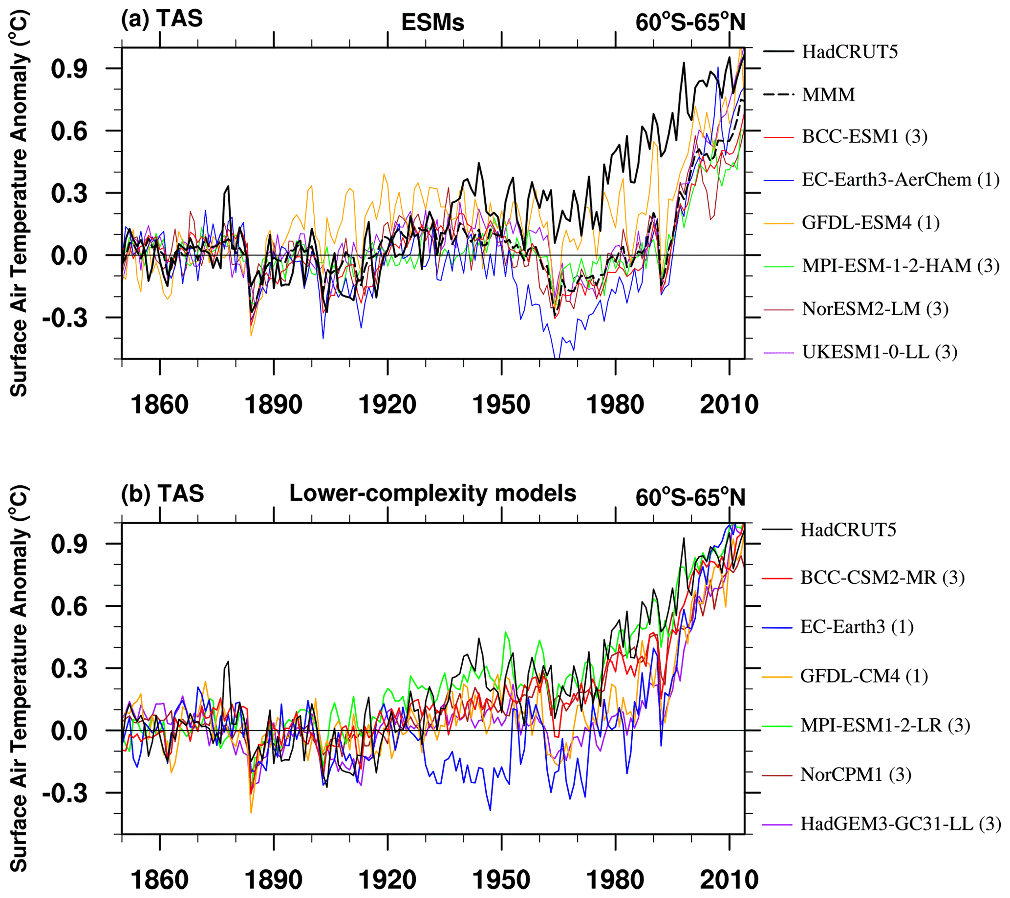
Figure 1(a) Historical near-global mean (60∘ S to 65∘ N) surface air temperature (TAS) anomalies relative to 1850–1900 mean from HadCRUT5 (thick black line), the ensemble mean for each ESM (solid color lines), and multi-model mean (MMM, dashed black line). Panel (b) is the same as panel (a) but for the lower-complexity models. Units: ∘C. Value in bracket is the number of available members for each model.
Decomposition of the ARI, the cloud-amount term, and cloud-albedo term of ACI is detailed further in the Appendix. The aerosol–cloud feedbacks are mainly in the ACI term which includes cloud spatial extent (amount), cloud albedo on radiative fluxes, and cloud particle swelling by humidification (Christensen et al., 2017; Neubauer et al., 2017). There is also a (smaller) effect of feedback on the ARI term that is also affected by cloud-amount changes insofar as increased/decreased cloud cover can obscure/reveal clear-sky radiative fluxes. We acknowledge that the linear approximation in our method does not explicitly account for the absorption above clouds or the adjustments to aerosol–radiation interactions (e.g., Carslaw et al., 2013) that are known to be locally important. Our formulation explicitly assumes that there is a broadly linear relationship between (i) loadSO4 and emissions and (ii) aerosol radiation with loadSO4 (and non-linearity due to cloud albedo or amount or any interaction is small at global scale as suggested in Booth et al., 2018). Should these interaction terms be non-negligible in this analysis, we still expect the broader attribution of the reasons for the model diversity in temperature response over the PHC period, either how they simulate aerosol concentrations or how they simulate the response to this, to generally hold.
This decomposition method is an approximate approach designed to be used with existing simulations, rather than a strict decomposition by dedicated simulations/output variables not included in CMIP6. It cannot tell us precise information about each interaction and adjustment, but it can give us an indication of why models behave differently.
Figure 1a shows the near-global averaged time series of the annual mean TAS anomaly relative to 1850 to 1900 in HadCRUT5 during the historical period from 1850 to 2014, as well as the ensemble means for each model except for EC-Earth3-AerChem and GFDL-ESM4 (where only a single realization is available for the hist-piAer experiment). The unforced, long-term drifts in TAS may occur in some of the ESMs, as estimated by their control simulation under pre-industrial conditions (Yool et al., 2020). We have not accounted for long-term control simulation drifts in our study as we are assuming that our focus on inter-decadal-scale variability of TAS anomalies is likely to be fairly insensitive to any century-scale drifts.
The TAS anomaly in HadCRUT5 is generally above the baseline climate from the 1940s onwards and warms fastest from the 1980s to 1990s. Compared with the observations, all the ESM simulations have negative TAS anomaly biases after the 1940s, which are also evident in the ensemble-mean historical TAS of 25 CMIP6 models with and without interactive chemistry schemes (Flynn and Mauritsen, 2020). In the ESMs and their ensemble mean (MMM), the cold anomaly biases resemble a pothole shape (Fig. 1a), which is relatively small before the 1950s and after the 2000s but prominent from the 1960s to 1990s. To reduce the impact of the change in the spatial pattern of the emissions in the late 20th century and the Pinatubo eruption in the early 1990s, we mainly focus on the excessively cold anomaly from 1960 to 1990 in this study. The impacts from the Agung (1963) and El Chichón (1982) eruptions have been left in the PHC period as their effect on the simulated temperature is not as pronounced as the response to Pinatubo and are short-lived in time compared to the period we study. The period of anomalous cold in the global mean from 1960 to 1990 in model simulations is defined as the pothole cooling (PHC). Table 3 shows the TAS anomaly biases in two periods: the pre-PHC period (1929–1959) and the PHC period (1960–1990). The cold bias in the MMM is −0.14 in the pre-PHC period and intensified to −0.40 in the PHC period. The PHC bias ranges from −0.20 to −0.58 ∘C among the ESMs with a standard deviation of 0.11 ∘C. Intra-model spread of PHC is relatively smaller. That is, model structural uncertainty is more responsible for PHC than internal climate variability.
The PHC bias is generally smaller in the corresponding lower-complexity models (Fig. 1b and Table 3). For models with prescribed chemistry and aerosol (BCC-CSM2-MR and MPI-ESM1-2-LR), the TAS anomaly is reasonably reproduced during the pre-PHC period and the PHC period. The PHC bias is large (−0.37 ∘C) in EC-Earth3, which has prescribed chemistry and aerosol. The large bias may be a reflection of the large internal variability on TAS in EC-Earth3 (Döscher et al., 2021), for which we have only one member. For models with a prescribed chemistry and interactive aerosol scheme (GFDL-CM4 and HadGEM3-GC31-LL), the cold biases during the PHC period are comparable with that in the corresponding ESMs.
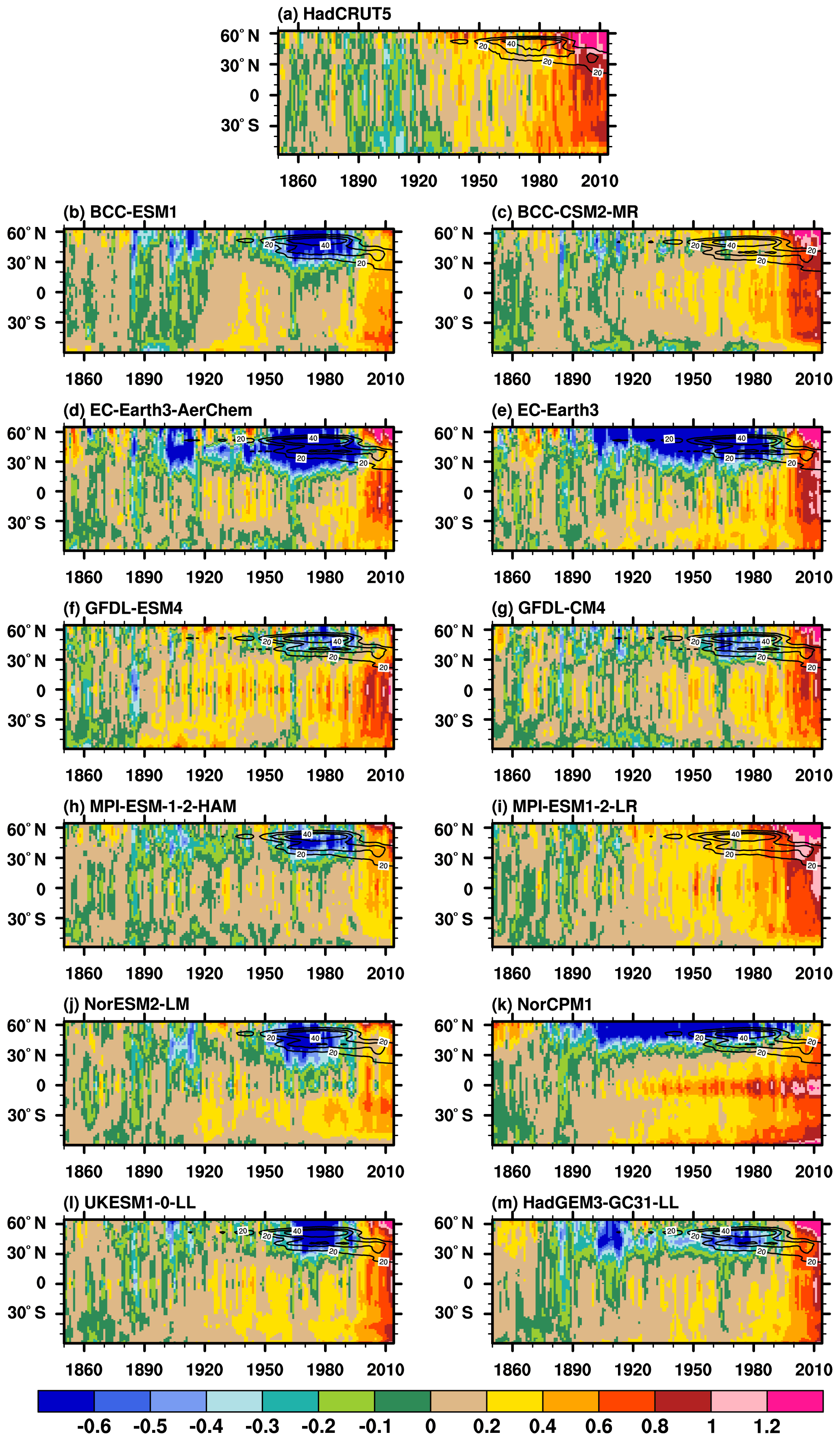
Figure 2Time–latitude cross section for annual-mean TAS anomalies (shaded) from (a) HadCRUT5, the ensemble mean for each ESM (b, d, f, h, j, and l), and the corresponding lower-complexity model (c, e, g, i, k, and m). The anomalies are related to the 1850–1900 mean. Units: ∘C. Note that the color scale intervals in the positive and negative directions are 0.2 and −0.1 ∘C, respectively. Line contours range from 20 to 40 with an interval of 10 showing the zonal mean anthropogenic surface SO2 emission provided by CMIP6.
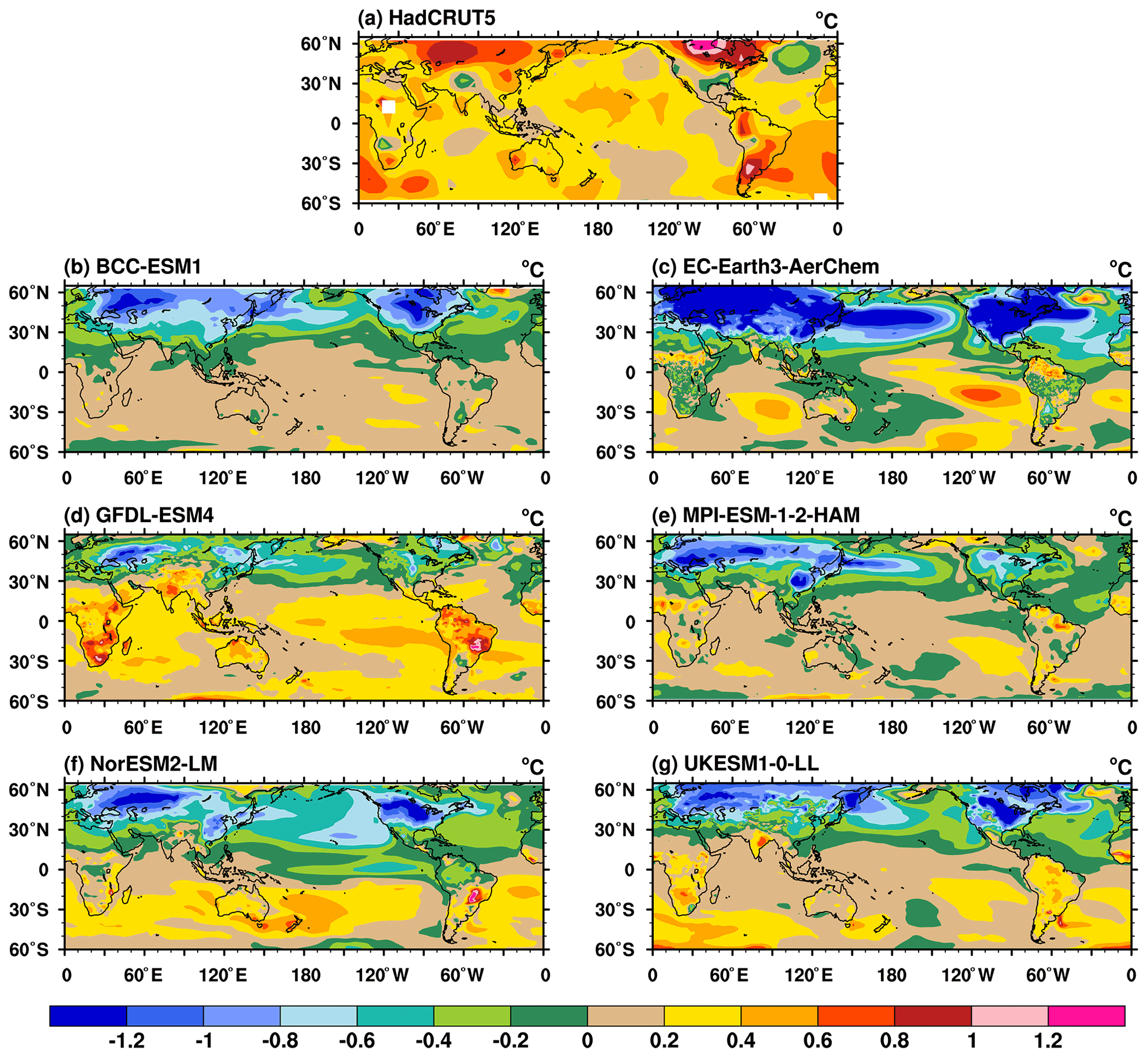
Figure 3The TAS anomalies during the pothole period (1960–1990) from (a) HadCRUT5 and (b–g) the ensemble mean for each ESM. The anomalies are relative to the 1850–1900 mean. Units: ∘C.
The spatial and temporal evolution of annually averaged TAS anomalies are further examined (Fig. 2). In HadCRUT5, TAS anomalies are generally positive after the 1940s. The most significant TAS anomalies are evident in the late 20th century and at the beginning of the 21st century, especially over the NH midlatitudes. The results from BCC-CSM2-MR and MPI-ESM1-2-LR agree well with the observations. However, the ESMs and the other lower-complexity models simulate pronounced cold anomalies over NH subtropical-to-high latitudes during the PHC period. The overestimated tropical and southern hemispheric warming in NorCPM1 offsets most of the cooling biases over NH subtropical-to-high latitudes.
Surface anthropogenic SO2 emissions rapidly increase during the PHC period (the line contours in Fig. 2). The latitudes of the cooling centers in the ESMs and lower-complexity models with an interactive aerosol scheme are spatially co-located with the SO2 emission sources – North America and East Asia (at around 30∘ N) and western Europe (at around 50∘ N). Generally, the different behaviors seen in Figs. 1 and 2 suggest that aerosol forcings may be overestimated in the ESMs and lower-complexity models with an interactive aerosol scheme, and the anomalous cooling is a result of the extra complexity associated with aerosol processes.
During the PHC period, the TAS anomalies in HadCRUT5 are generally positive and are the largest over Eurasia and North America (Fig. 3a). The warm anomalies are on average more than 0.4 ∘C along the 30–60∘ N latitudinal belt. However, the ESMs show anomalies with the opposite sign (Fig. 3b–g) as do the lower-complexity models with an interactive aerosol scheme (figures not shown). The PHC is pronounced over major SO2 emission centers (western Europe, East Asia, and the eastern US) and their downstream regions. The cold anomalies over Eurasia and North America are lower than −0.6∘C in the ESMs. The PHC biases are strongest at lower levels (figures not shown), which is distinct from the amplified upper-tropospheric warming response to greenhouse gases.
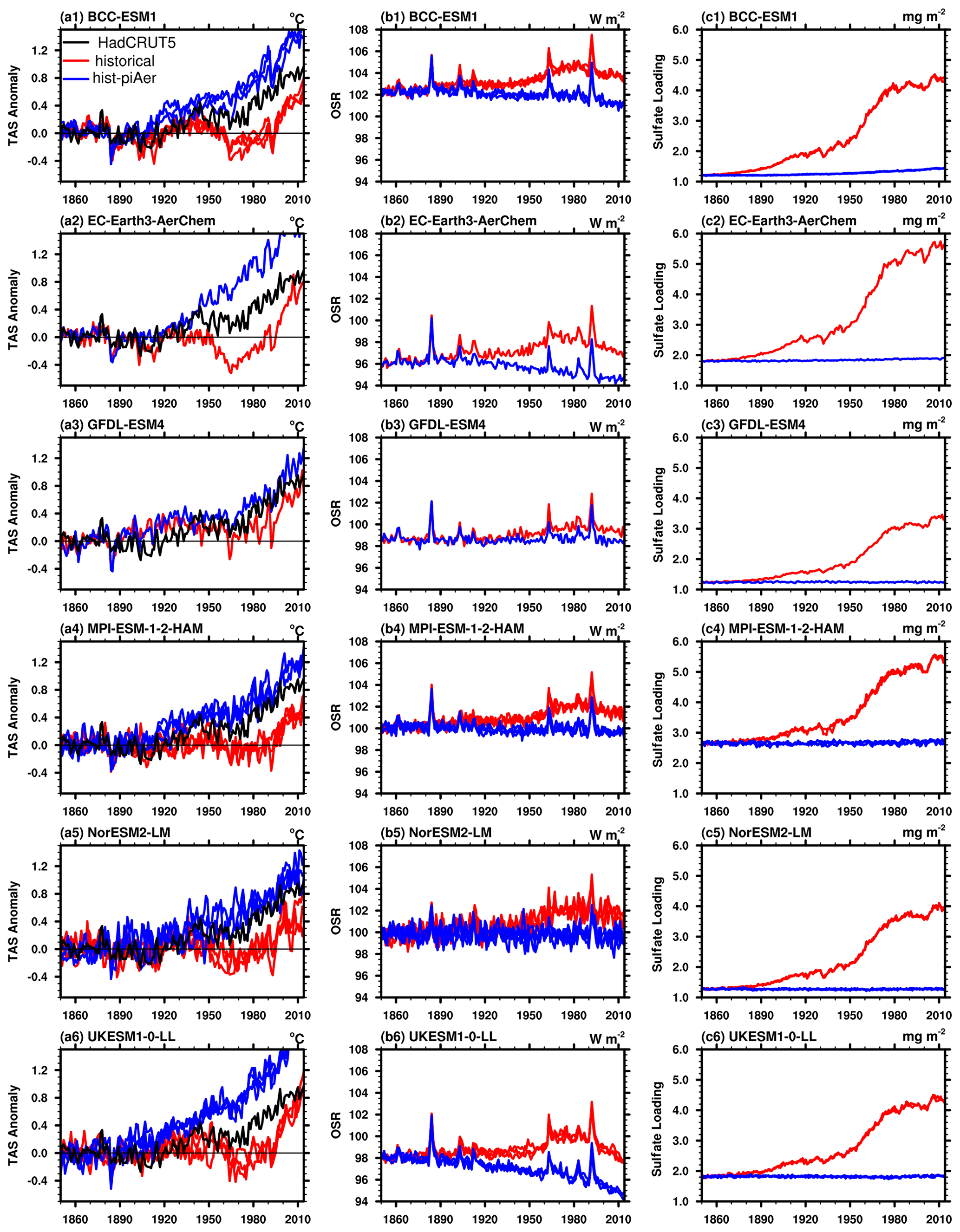
Figure 4Evolutions of global annual means of (a1–6) TAS anomalies (left panel, units: ∘C), (b1–6) outgoing shortwave radiation at TOA (OSR, middle panel, units: W m−2), and (c1–6) sulfate loading (right panel, units: mg m−2) in HadCRUT5 (black line), with each ESM member of the historical (red lines) and hist-piAer experiments (blue lines). The TAS anomalies are relative to the 1850–1900 mean.
The differences between the historical and hist-piAer simulations help to investigate the impact of anthropogenic aerosol emissions and their possible contribution to the PHC biases. In this section, we examine the TAS, OSR, and sulfate loading differences and look in detail at their relationship. As shown by the evolution of TAS anomalies in the two experiments (Fig. 4a1–6), during the PHC period, TAS anomalies in HadCRUT5 (black line) are higher than those in the historical members but lower than those in the hist-piAer members in all ESMs. That is, the model responses to anthropogenic aerosol emissions are larger than the amplitude of the PHC. The temporal evolution of the OSR corresponds with that of the TAS but occurs in the opposite direction (Fig. 4b1–6). The sulfate loading differences are relatively small in the 19th century, mildly increase in the first half of the 20th century, grow most rapidly during the PHC period, and remain high afterward (Fig. 4c1–6). The growing sulfate loading during the PHC period corresponds with the increase in Northern Hemisphere anthropogenic surface SO2 emissions (line contours in Fig. 2). In comparison with the TAS and OSR differences, the intra-model spread of sulfate loading for each ESM is relatively small. However, the inter-model diversity of sulfate loading is large. For example, the sulfate loading difference between the historical and hist-piAer experiments around the year 2000 is about 4 mg m−2 in EC-Earth3-AerChem, almost twice of that in GFDL-ESM4. With similar anthropogenic SO2 emission rates, the lower sulfate loading difference in GFDL-ESM4 indicates it has a shorter sulfate aerosol residence time than that in EC-Earth3-AerChem, which may be due to their different sulfate production and deposition schemes. The sulfate loading diversity is also evident in CMIP5 models and is partly responsible for the diversity in modeled radiative forcing (Wilcox et al., 2015).
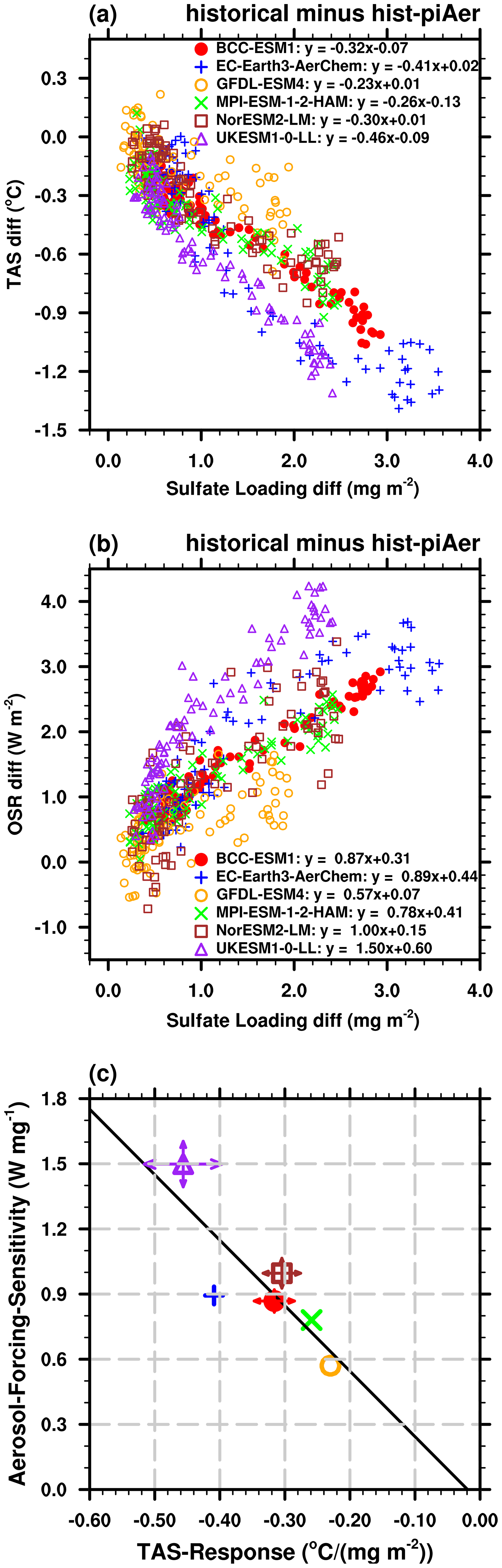
Figure 5Scatter plots of 1900–1990 yearly sulfate loading differences between the historical and hist-piAer simulations (x axis) versus (a) TAS differences and (b) OSR (y axis). Results are from the ensemble mean for each ESM. The captions are the linear fitting equations. Panel (c) shows the TAS response (x axis) and aerosol forcing sensitivity (y axis) which is equal to slope of linear fitting for each ESM (markers), as well as the corresponding intra-model spread (arrows).
The latitudinal movement of the SO2 emission center from the 1990s affects the relative strength of aerosol forcing. Due to the more rapid oxidation and higher incoming solar flux at lower latitudes, an equatorward shift in SO2 emissions around the 1990s results in a more efficient production of sulfate and stronger aerosol forcing (Manktelow et al., 2007). The northern midlatitude temperature is also more sensitive to the distribution of aerosols, which is approximately twice as large as the global average (Collins et al., 2013; Shindell and Faluvegi, 2009). Therefore, we focus on the relationships between TAS, OSR, and sulfate loading after 1900 when SO2 emission changes are dominated by its anthropogenic component, as well as before 1990. As shown in Fig. 5a, the TAS differences between the historical and hist-piAer simulations vary approximately linearly with the differences in the sulfate loading. The OSR differences are approximately linearly correlated with sulfate loading differences (Fig. 5b). In both cases, the approximation of linearity holds less well for UKESM1-0-LL, especially at small sulfate loadings. This reflects the behavior of HadGEM2, a predecessor of UKESM1-0-LL (Wilcox et al., 2015), and is likely to be due to the strong aerosol–cloud-albedo effect in these models. The global mean annual mean reff decreases by about 0.7 µm since pre-industrial era – more than twice the magnitude of change seen in the other models (Fig. 1b in Wilcox et al., 2015; Fig. 9b in this study).
The slope of the linear fitting equation between TAS (OSR) and sulfate loading as shown in the captions in Fig. 5a (Fig. 5b) is a measure of the sensitivity of TAS (aerosol forcing) to perturbations in atmospheric aerosol. Moreover, TAS response and aerosol forcing sensitivity are linearly correlated across the ESMs (Fig. 5c). That is, the strength of the TAS response can be understood as the magnitude of aerosol forcing sensitivity within each ESM. The TAS response and aerosol forcing sensitivity is the lowest in GFDL-ESM4. The TAS response and aerosol forcing sensitivity in UKESM1-0-LL (the purple marker in Fig. 5c) are the strongest, as well as their intra-model spread (the length of arrows), indicating that TAS and aerosol forcing in this model are relatively more susceptible to changes in aerosol.
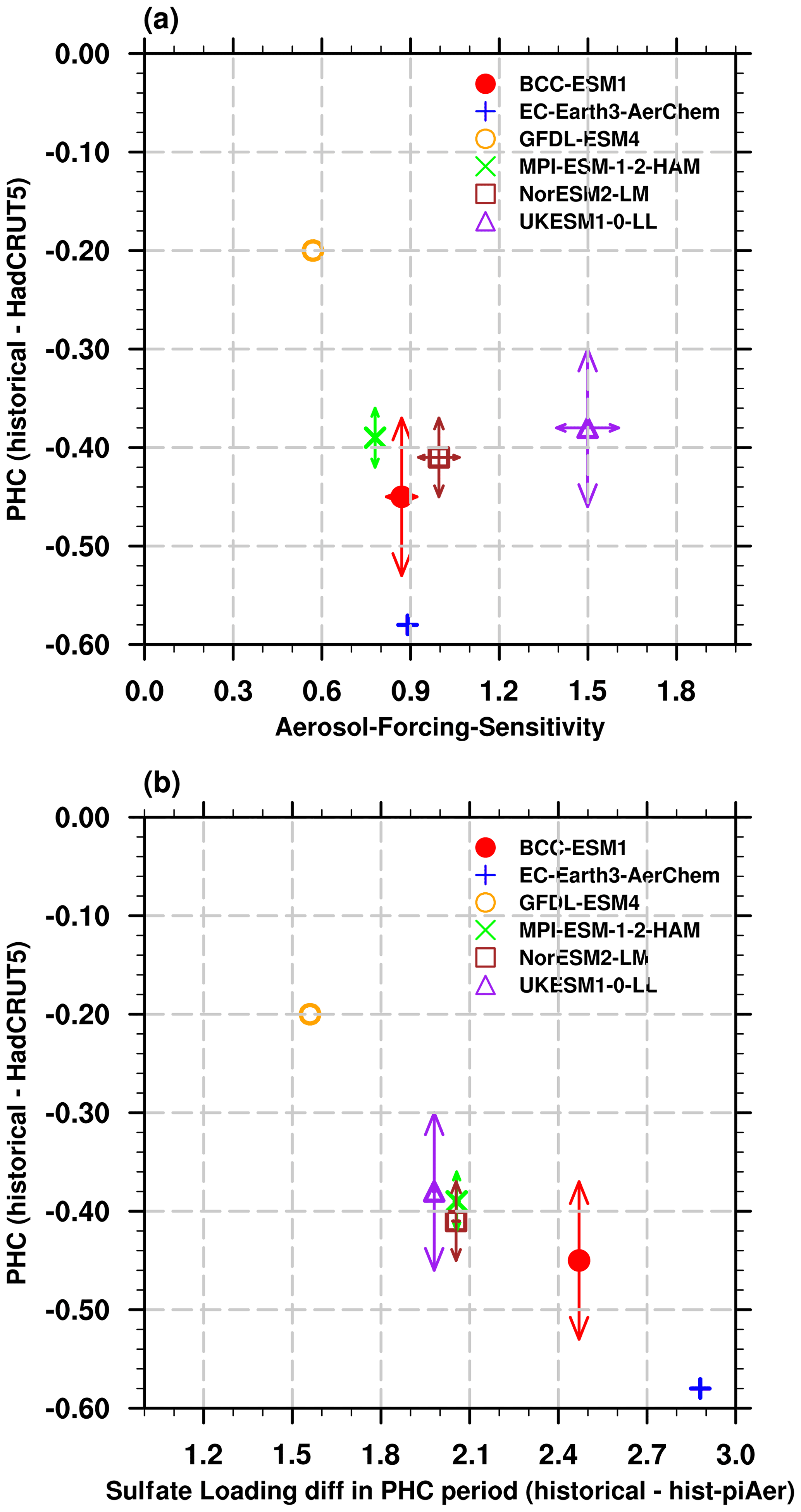
Figure 6Pothole cooling (PHC) bias in ESMs (∘C) versus (a) the aerosol forcing sensitivity (W mg−1) and (b) sulfate loading differences (mg m−2) during the PHC period. The arrows show the uncertainty ranges among the members in each ESM.
Considering the close relationship between TAS anomalies and aerosol loading (Fig. 5a), as well as the impact of aerosol forcing sensitivity on the TAS response in ESMs (Fig. 5c), their relative contributions to the PHC biases are examined. Figure 6a shows the PHC biases versus the aerosol forcing sensitivity (markers) and their intra-model spread (arrows). GFDL-ESM4 has the weakest aerosol forcing sensitivity (∼ 0.60 W mg−1) and the smallest PHC (−0.20 ∘C). However, the relationship between the PHC biases and the aerosol forcing sensitivity among the ESMs is not clear: ESMs have similar PHC biases (MPI-ESM-1-2-HAM, NorESM2-LM, and UKESM1-0-LL) that show large differences in the aerosol forcing sensitivity, ranging from 0.78 to 1.5 W mg−1; the aerosol forcing sensitivity in EC-Earth3-AerChem is close to that in BCC-ESM1, but the PHC is more than 0.1 ∘C lower; and the aerosol forcing sensitivity in UKESM1-0-LL is the strongest (∼ 1.5 W mg−1) but not the PHC bias. Therefore, the aerosol forcing sensitivity is not able to explain the different PHC biases among ESMs.
As shown in Fig. 6b, the sulfate loading differences between the historical and hist-piAer experiments during the PHC period are large among ESMs (the x axis), which are about 1.5 mg m−2 in GFDL-ESM4 but approximately 2.9 mg m−2 in EC-Earth3-AerChem. The sulfate loading differences during the PHC period and PHC biases show a negative correlation: the PHC bias is generally larger in models with higher sulfate loading over this period; the ESMs with similar PHC biases (MPI-ESM1-2-LR, NorESM2-LM, and UKESM1-0-LL) show similar aerosol loading differences. Therefore, the excessive cooling during the PHC period and the inter-model diversity in ESMs are attributed to the higher aerosol burden in these models.
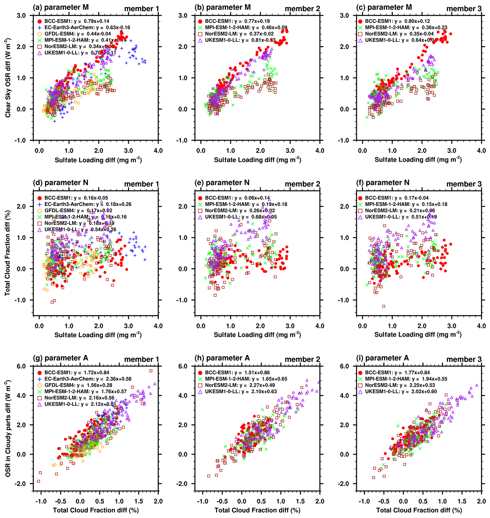
Figure 7Annual mean differences between the historical and hist-piAer simulations in the ESM members during the 1900–1990 period for (a–c) sulfate loading (mg m−2) versus clear-sky OSR (OSRclr, W m−2), (d–f) sulfate loading versus total cloud fraction (%), and (g–i) total cloud fraction versus OSR in cloudy parts (W m−2). Slopes of the linear fitting equations from the top row to the bottom row refer to the parameters M, N, and A, respectively.
5.1 The proportions of ARI and ACI
Although the aerosol forcing sensitivity is not responsible for the anomalous cooling biases in ESMs, it is a good way to identify model differences in the response to aerosol changes. As shown in Fig. 5c, there are significant differences in the aerosol forcing sensitivity among ESMs. The aerosol forcing sensitivity in UKESM1-0-LL is almost 3 times of that in GFDL-ESM4. Due to the uncertainties in physical processes and cloud parameterizations, the dominant component (ARI or ACI) of aerosol forcing sensitivity may also vary among ESMs. Here, we separate the different components of the aerosol forcing sensitivity in each ESM by the method introduced in the Sect. 2.3 and the Appendix. Sulfate loading is used as a proxy of aerosol amount for all aerosol components in the quantification of the total effect because of its dominant contribution to anthropogenic aerosol load during this period and its covariation with the other aerosol species.
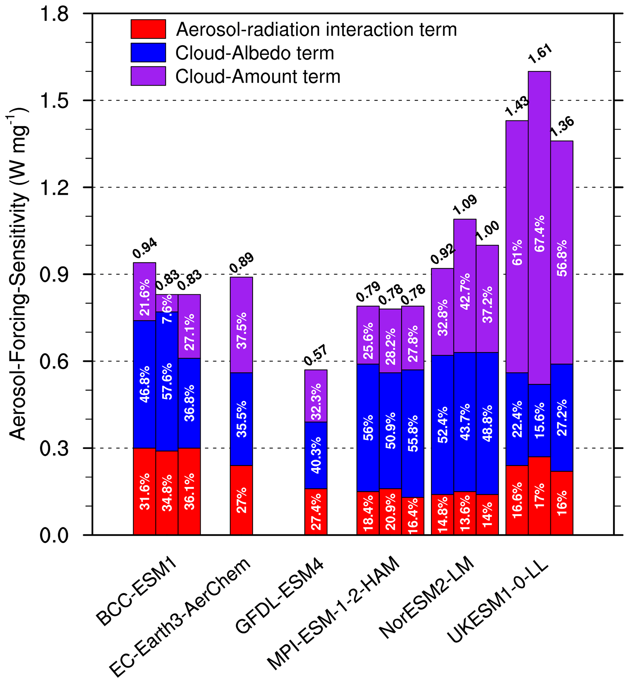
Figure 8Total aerosol forcing sensitivity from each member in ESMs. The number marked on the top is the total aerosol forcing sensitivity. Partitions of aerosol–radiation interaction term, cloud-albedo term, and cloud-amount term are marked in the corresponding color bars. Unit: W mg−1. Where multiple realizations are available for a model, a bar is shown for each member.
The ARI can be approximated to , where CLT_hist is cloud amount in the historical simulation and parameter M is a measure of the strength of aerosol–radiation interactions (). Parameter M varies widely from about 0.35 W mg−1 in NorESM2-LM to about 0.79 W mg−1 in BCC-ESM1 (captions in Fig. 7a–c). Since parameter M does not change much among ensemble members in each ESM, their ARI is similar across members. That is, the impact of internal climate variability on the ARI is relatively small, which is consistent with the quantitative analysis in Fig. 8 (red bars).
The ACI can be estimated from the difference between the aerosol forcing sensitivity and the ARI. The proportion of the aerosol forcing sensitivity arising from the ACI is higher than 64 % in all ESMs (Fig. 8). The inter-model variation of the ACI (0.37 W mg−1) is much larger than that for the ARI (0.09 W mg−1). For example, the ACI in UKESM1-0-LL (∼ 1.2 W mg−1) is higher than all the others and is about 3 times of that in GFDL-ESM4 (0.41 W mg−1). This demonstrates that differences in the aerosol forcing sensitivity across the ESMs are dominated by the differences in their individual representation of ACI. Chen et al. (2014) also suggested that ACI is the main contribution to the aerosol radiative forcing uncertainty, and the response of marine clouds to aerosol changes is paramount. The intra-model variations in the ACI are also larger than that for the ARI. That is because the intra-model variations of the ACI are influenced by the effects of climate system internal variability on aerosol-induced cloud microphysics, with cloud radiative properties and cloud lifetimes varying regionally. The intra-model variations are also attributable to the differences in atmospheric circulation among different ensemble members, which may affect the geographical distributions of aerosols and clouds and lead to a different magnitude of interactions.
The quantitative analysis in Fig. 8 also indicates that ESMs with similar aerosol forcing sensitivity may have different contributions from ARI and ACI. The aerosol forcing sensitivity is similar in BCC-ESM1, EC-Earth3-AerChem, MPI-ESM-1-2-HAM, and NorESM2-LM, but the fractional contribution from the ACI is the largest in NorESM2-LM, and its ARI is less than half of that in BCC-ESM1. Generally, BCC-ESM1 has the largest fractional ARI contribution (34 %), whereas NorESM2-LM has the largest fraction of ACI contribution (86 %).
5.2 The proportions of cloud-amount and cloud-albedo terms
Our ACI metric includes several mechanisms by which aerosols can alter cloud properties. This includes the cloud-albedo effects (or Twomey effect), referred to as the radiative forcing part of ACI, and effects of aerosols on the macroscopic properties of clouds (for example, cloud extent and lifetime), referred to as the adjustment part of ACI. However, it is complicated to separate these two parts of ACI directly using available CMIP6 diagnostics, because the former is most accurately defined as a change in cloud albedo with all other cloud properties held constant (i.e., a change in cloud-droplet number concentration only), whilst the latter allows cloud properties to respond.
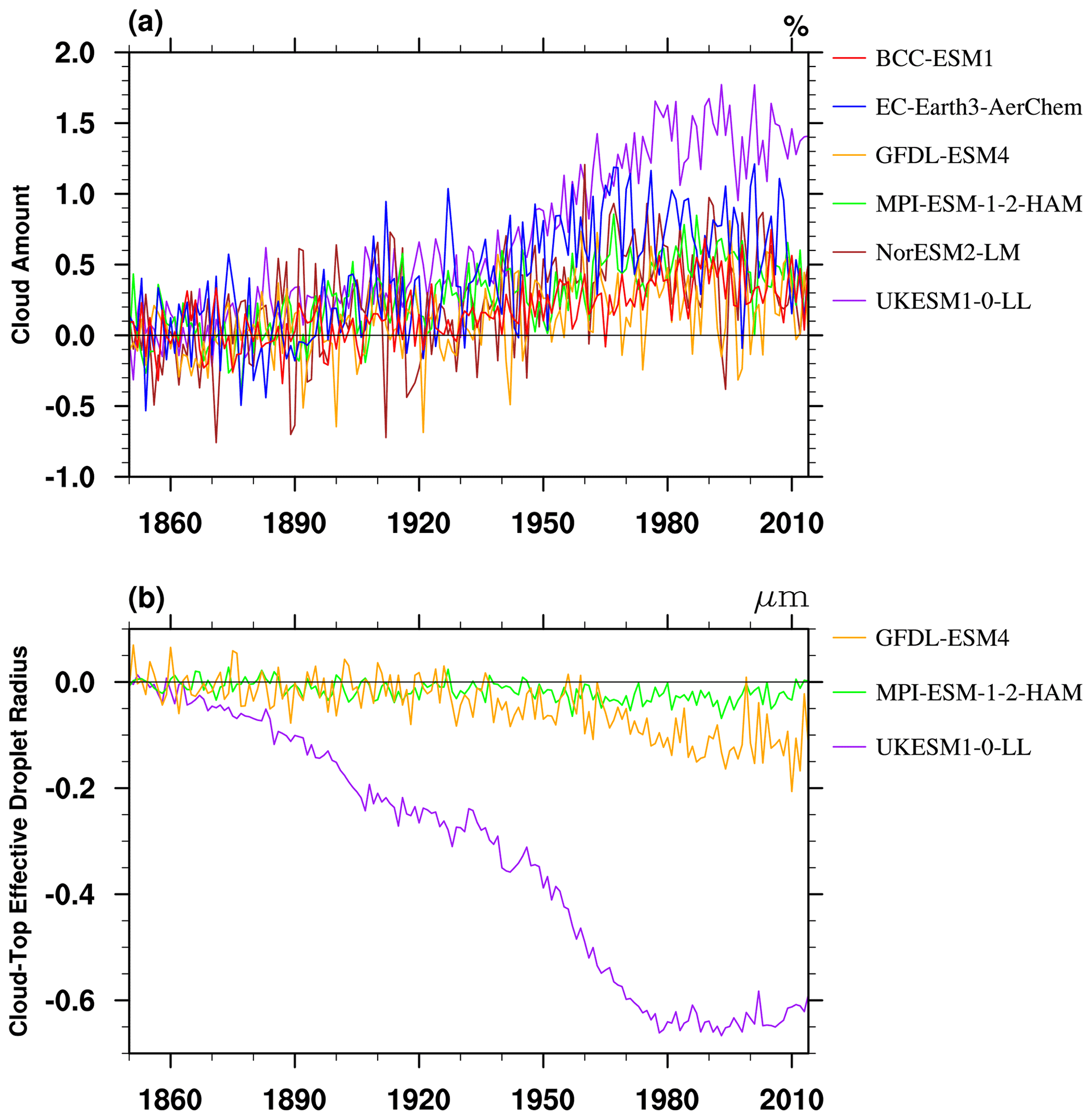
Figure 9(a) Evolutions of global mean cloud-amount differences between the historical and hist-piAer simulations in ensemble mean for each ESM (units: %). Panel (b) is the same as panel (a) but for cloud-top effective droplet radius (reff, µm). The reff data are only available for GFDL-ESM4, MPI-ESM-1-2-HAM, and UKESM1-0-LL.
Figure 9 shows the evolution of global mean differences in total cloud amount (ΔCLT) and cloud-top effective droplet radius (Δreff) between the historical and hist-piAer experiments. The ΔCLT and Δreff in UKESM1-0-LL are the largest and highly correlated with each other (with a correlation coefficient of −0.92 during the 1900 to 1990 period). For the other two ESMs for which Δreff was archived, the correlation coefficient is −0.40 for MPI-ESM-1-2-HAM and insignificant for GFDL-ESM4 (−0.09). The ΔCLT and Δreff differences are smaller in MPI-ESM-1-2-HAM and GFDL-ESM4 than in UKESM1-0-LL, especially for the Δreff differences. Δreff is generally related to the cloud optical depth and cloud water path, and ΔCLT is related to adjustments in cloud cover due to ACI. Therefore, the radiative forcing part and adjustment part of ACI may be closely coupled in UKESM1-0-LL and are hard to separate statistically. The strong correlation between cloud amount and reff response in UKESM1-0-LL indicates that this model is sensitive to aerosol–cloud interactions, which likely contributes to it having the strongest aerosol forcing sensitivity and intra-model spread of all the CMIP6 models (Fig. 5c). MPI-ESM-1-2-HAM and UKESM1-0-LL have similar ensemble mean PHC biases and close sulfate burden, but the aerosol forcing sensitivity difference in UKESM1-0-LL is almost twice of that in MPI-ESM-1-2-HAM (Fig. 5). That is, the overestimated sulfate burden dominates the PHC biases, but the ACI sensitivity may partly affect the amplitude and uncertainty ranges of PHC biases.
Despite of the closely coupled radiative forcing part and adjustment part of ACI in UKESM1-0-LL, it is still possible to split the ACI into a part that is correlated with cloud-amount differences and a residual term. This can be done statistically by regressing out the approximate linear dependence of the differences between historical and hist-piAer simulations of the cloudy part of OSR (OSRcld_p) on cloud fraction in each ESM (parameter A in Fig. 7g–i). We call the degree of linear correlation of ΔOSRcld_p with ΔCLT the “cloud-amount term”, and the residual will be referred to as the “cloud-albedo term”. However, we reiterate that the so-called “cloud-amount term” may also include changes in the reflectivity of clouds if these are correlated with changes in cloud amount. Similarly, the cloud-albedo term will contain any sources of cloud-amount changes which have not been removed by linearly regressing OSRcld_p against cloud amount. As such, we do not intend for this nomenclature to indicate a precise separation of the radiative forcing part and adjustment part of ACI. Our decomposition allows first-order assessment of these terms from historical simulations without the need for extra simulations or calls and also allows estimates from observations and intermodel comparisons.
As described in the Sect. 2.3 and the Appendix, the cloud-amount term is sensitive to two parameters: the cloud-amount response (parameter N in Fig. 7d–f) and the sensitivity of OSR reflected from clouds to cloud-amount changes (parameter A, Fig. 7g–i). As shown in Fig. 8, UKESM1-0-LL has the largest contribution of the cloud-amount term to aerosol forcing sensitivity (62 %, 0.91 W mg−1); the cloud-amount term is the smallest in GFDL-ESM4 (∼ 0.18 W mg−1). The cloud-albedo term is defined to be linearly independent of cloud-amount changes (adjustments). For the CMIP6 ESMs, it can only be estimated as the residual after subtracting the cloud-amount term from the ACI. The cloud-albedo term is similar in BCC-ESM1, MPI-ESM-1-2-HAM, and NorESM2-LM. The inter-model variation for the cloud-amount term is about twice of that for the cloud-albedo term (0.29 W mg−1 vs. 0.16 W mg−1). That is, the variations of cloud-amount term are the major source of inter-model ACI (and the aerosol forcing sensitivity) differences between ESMs. Therefore, difference in the cloud-amount terms, across the ESMs, dominates the uncertainties in the aerosol forcing sensitivity.
Note that our definitions do not correspond to the effects measured by using multiple calls to the radiation scheme of a model, with and without aerosols, which measure instantaneous radiative effects; multiple calls give a measure of the fast response of clouds to aerosol perturbations in a fixed thermodynamic and dynamical background, allowing for a clear separation between ACI and rapid adjustments (e.g., Bellouin et al., 2013). This differs from aerosol forcing diagnosed by differencing climate projections with different aerosol forcings, which include the slow effects of other feedbacks. For example, differences in climate forcings can lead to different SST patterns, which in turn alter the location and characteristics of clouds. Despite these differences, an advantage of our classification is that it provides a possible method for model evaluation since the variables used are also, in principle, available from the observations.
This study focuses on the reproduction of historical surface air temperature anomalies in six CMIP6 ESMs. The ESMs systematically underestimate TAS anomalies relative to 1850 to 1900 in the NH midlatitudes, especially from 1960 to 1990, the pothole cooling (PHC) period. Previous studies suggested that aerosol cooling is too strong in many CMIP6 models. Our study more specifically found that the PHC is concurrent in time and space with anthropogenic SO2 emissions, which rapidly increase in the PHC period in NH. Models with larger aerosol burdens have larger PHC biases. The primary role of aerosol emissions in these biases is further supported by the differences between ESMs and the lower-complexity models with prescribed aerosol.
Differences between historical simulations and simulations with aerosol emissions fixed at their pre-industrial levels (hist-piAer) are used to isolate the impacts of industrial aerosol emission. We propose that the overestimated aerosol concentrations in the ESMs are responsible for the spurious drop in TAS in the mid-20th century, rather than a high sensitivity of the models to aerosol forcing. Although the aerosol forcing sensitivity differences in ESMs cannot explain the PHC biases, they are a good measurement of aerosol effects that can be used to explore structural differences between models. A simple metric is derived for determining the dominant contribution to the aerosol forcing sensitivity in any specific model: ARI or ACI. The ACI accounts for more than 64 % of the aerosol forcing sensitivity in all analyzed ESMs. The considerable inter-model variation in the aerosol forcing sensitivity is mainly attributable to the uncertainty in the ACI within models. The ACI can be further decomposed into a cloud-amount term and a cloud-albedo term. The cloud-amount term is found to be the major source of inter-model diversity of ACI. Considering the crucial role of cloud properties on the inter-model spread in aerosol forcing sensitivity, the aerosol–cloud interactions should be a focus in the development of aerosol schemes within ESMs.
Considering the dominant role of sulfate aerosol on anthropogenic aerosol forcing, we use the sulfate loading (loadSO4) as a proxy for all aerosol in our analysis. The aerosol forcing sensitivity (as determined by the difference between the historical and hist-piAer experiments) is estimated by the all-sky OSR differences per sulfate burden unit (), and it is the combination of OSR differences in the clear-sky parts () and the cloudy parts ():
The OSRclr_p for a particular experiment can be calculated as
where CLT is the total cloud amount (unit: %), and OSRclr is the OSR assuming all clear sky (unit: W m−2). The cloud-amount changes (ΔCLT) will modify the proportion of clear sky and then affect the OSR changes attributed to the clear-sky part by covering or uncovering aerosols in clear sky. Therefore, based on Eq. (A2), can be decomposed into the OSRclr response () and CLT response ():
where CLT_hist and OSRclr_hist are the mean CLT and OSRclr in the historical experiment. Residual_clr is the residual term that is non-linear in ΔOSRclr and ΔCLT. The parameter is related to the strength of the aerosol–radiation interaction and can be estimated by linear fitting of ΔOSRclr on ΔloadSO4. The parameter is related to CLT response and estimated by linear fitting of ΔCLT on ΔloadSO4. Therefore, the first term on the right-hand side of Eq. (A3), , corresponds to the aerosol radiative effect; the second term, , corresponds to the impact of changes in the clear-sky area.
The OSRcld_p is the cloudy part of OSR, accounting for the difference between OSR and OSRclr_p. The cloudy part of the OSR differences (ΔOSRcld_p) can be generally estimated as
where the parameter is the sensitivity of the shortwave flux reflected by clouds to changes in cloud amount. The parameter A depends on the baseline cloud albedo (radiative flux per cloud-amount unit) and can be estimated by linear fitting of ΔOSRcld_p on ΔCLT. Hence,
where N is the parameter defined above. Therefore, the first term on the right-hand side of Eq. (A4), A⋅N, corresponds to the impact of cloud-amount changes on the cloud radiation; and the cloud-albedo term can be obtained as a residual after subtracting A⋅N from , thereby eliminating any linear dependence of the cloudy-sky shortwave flux response on cloud-amount changes.
As with the clear-sky decomposition, residual_cld is a possible non-linear term and is assumed to be small. This term cannot in fact be distinguished from the cloud-albedo term in this analysis: we must therefore accept that cloud-albedo changes could be accompanied by non-linear changes in macroscopic cloud properties (in this framework).
The total aerosol forcing sensitivity can be measured by substituting the derived values of from both the clear sky (Eq. A3) and cloudy (Eq. A4) parts back into Eq. (A1):
Based on Eq. (A5), the total aerosol forcing sensitivity can therefore be decomposed to the aerosol–radiation interaction term (ARI), , cloud-amount term as including the impacts of cloud-amount changes on aerosol radiation () and cloud radiation (A⋅N), and cloud-albedo term (defined as a residual).
All the model data can be freely downloaded from the Earth System Grid Federation (ESGF) nodes (https://esgf-node.llnl.gov/search/cmip6/) (WCRP, 2021). The global historical surface temperature anomalies HadCRUT5 dataset is freely available on https://www.metoffice.gov.uk/hadobs/hadcrut5/data/current/download.html (Met Office Hadley Centre, 2021).
The main ideas were developed by JZ, KF, STT, JPM, and TW. JZ, KF, and STT wrote the original draft, and the results were supervised by LJW, BBB, and DS. All the authors discussed the results and contributed to the final paper.
The contact author has declared that neither they nor their co-authors have any competing interests.
Publisher's note: Copernicus Publications remains neutral with regard to jurisdictional claims in published maps and institutional affiliations.
This article is part of the special issue “The Aerosol Chemistry Model Intercomparison Project (AerChemMIP)”. It is not associated with a conference.
All the authors were supported by the UK–China Research and Innovation Partnership Fund through the Met Office Climate Science for Service Partnership (CSSP) China as part of the Newton Fund. Laura J. Wilcox was supported by the Natural Environment Research Council (NERC) North Atlantic Climate System Integrated Study (ACSIS) program.
This research has been supported by the National Key Research and Development Program of China (grant nos. 2018YFE0196000 and 2016YFA0602100).
This paper was edited by Jennifer G. Murphy and reviewed by two anonymous referees.
Aas, W., Mortier, A., Bowersox, V., Cherian, R., Faluvegi, G., Fagerli, H., Hand, J., Klimont, Z., Galy-Lacaux, C., Lehmann, C. M. B., Myhre, C. L., Myhre, G., Olivié, D., Sato, K., Quaas, J., Rao, P. S. P., Schulz, M., Shindell, D., Skeie, R. B., Stein, A., Takemura, T., Tsyro, S., Vet, R., and Xu, X.: Global and regional trends of atmospheric sulfur, Scient. Rep., 9, 953, https://doi.org/10.1038/s41598-018-37304-0, 2019.
Bellouin, N., Mann, G. W., Woodhouse, M. T., Johnson, C., Carslaw, K. S., and Dalvi, M.: Impact of the modal aerosol scheme GLOMAP-mode on aerosol forcing in the Hadley Centre Global Environmental Model, Atmos. Chem. Phys., 13, 3027–3044, https://doi.org/10.5194/acp-13-3027-2013, 2013.
Bethke, I., Wang, Y., Counillon, F., Kimmritz, M., Fransner, F., Samuelsen, A., Langehaug, H. R., Chiu, P.-G., Bentsen, M., Guo, C., Tjiputra, J., Kirkevåg, A., Oliviè, D. J. L., Seland, Ø., Fan, Y., Lawrence, P., Eldevik, T., and Keenlyside, N.: NCC NorCPM1 model output prepared for CMIP6 CMIP, Earth System Grid Federation [dataset], https://doi.org/10.22033/ESGF/CMIP6.10843, 2019.
Bindoff, N. L., Stott, P. A., AchutaRao, K. M., Allen, M. R., Gillett, N., Gutzler, D., Hansingo, K., Hegerl, G., Hu, Y. Y., Jain, S., Mokhov, I. I., Overland, J., Perlwitz, J., Sebbari, R., and Zhang, X. B.: Detection and Attribution of Climate Change: from Global to Regional, in: Climate Change 2013: The Physical Science Basis. Contribution of Working Group I to the Fifth Assessment Report of the Intergovernmental Panel on Climate Change, edited by: Stocker, T. F., Qin, D., Plattner, G.-K., Tignor, M., Allen, S. K., Boschung, J., Nauels, A., Xia, Y., Bex, V., and Midgley, P. M., Cambridge University Press, Cambridge, UK and New York, NY, USA.
Booth, B. B. B., Harris, G. R., Jones, A., Wilcox, L., Hawcroft, M., and Carslaw, K. S.: Comments on “Rethinking the Lower Bound on Aerosol Radiative Forcing”, J. Climate, 31, 9407–9412, https://doi.org/10.1175/jcli-d-17-0369.1, 2018.
Carslaw, K. S., Lee, L. A., Reddington, C. L., Pringle, K. J., Rap, A., Forster, P. M., Mann, G. W., Spracklen, D. V., Woodhouse, M. T., Regayre, L. A., and Pierce, J. R.: Large contribution of natural aerosols to uncertainty in indirect forcing, Nature, 503, 67–71, https://doi.org/10.1038/nature12674, 2013.
Charlson, R. J., Langner, J., and Rodhe, H.: Sulphate aerosol and climate, Nature, 348, 22–22, https://doi.org/10.1038/348022a0, 1990.
Chen, Y.-C., Christensen, M. W., Stephens, G. L., and Seinfeld, J. H.: Satellite-based estimate of global aerosol–cloud radiative forcing by marine warm clouds, Nat. Geosci., 7, 643–646, https://doi.org/10.1038/ngeo2214, 2014.
Christensen, M. W., Neubauer, D., Poulsen, C. A., Thomas, G. E., McGarragh, G. R., Povey, A. C., Proud, S. R., and Grainger, R. G.: Unveiling aerosol–cloud interactions – Part 1: Cloud contamination in satellite products enhances the aerosol indirect forcing estimate, Atmos. Chem. Phys., 17, 13151–13164, https://doi.org/10.5194/acp-17-13151-2017, 2017.
Collins, W. J., Fry, M. M., Yu, H., Fuglestvedt, J. S., Shindell, D. T., and West, J. J.: Global and regional temperature-change potentials for near-term climate forcers, Atmos. Chem. Phys., 13, 2471–2485, https://doi.org/10.5194/acp-13-2471-2013, 2013.
Collins, W. J., Lamarque, J.-F., Schulz, M., Boucher, O., Eyring, V., Hegglin, M. I., Maycock, A., Myhre, G., Prather, M., Shindell, D., and Smith, S. J.: AerChemMIP: quantifying the effects of chemistry and aerosols in CMIP6, Geosci. Model Dev., 10, 585–607, https://doi.org/10.5194/gmd-10-585-2017, 2017.
Dittus, A. J., Hawkins, E., Wilcox, L. J., Sutton, R. T., Smith, C. J., Andrews, M. B., and Forster, P. M.: Sensitivity of Historical Climate Simulations to Uncertain Aerosol Forcing, Geophys. Res. Lett., 47, e2019GL085806, https://doi.org/10.1029/2019gl085806, 2020.
Döscher, R., Acosta, M., Alessandri, A., Anthoni, P., Arneth, A., Arsouze, T., Bergmann, T., Bernadello, R., Bousetta, S., Caron, L.-P., Carver, G., Castrillo, M., Catalano, F., Cvijanovic, I., Davini, P., Dekker, E., Doblas-Reyes, F. J., Docquier, D., Echevarria, P., Fladrich, U., Fuentes-Franco, R., Gröger, M., v. Hardenberg, J., Hieronymus, J., Karami, M. P., Keskinen, J.-P., Koenigk, T., Makkonen, R., Massonnet, F., Ménégoz, M., Miller, P. A., Moreno-Chamarro, E., Nieradzik, L., van Noije, T., Nolan, P., O'Donnell, D., Ollinaho, P., van den Oord, G., Ortega, P., Prims, O. T., Ramos, A., Reerink, T., Rousset, C., Ruprich-Robert, Y., Le Sager, P., Schmith, T., Schrödner, R., Serva, F., Sicardi, V., Sloth Madsen, M., Smith, B., Tian, T., Tourigny, E., Uotila, P., Vancoppenolle, M., Wang, S., Wårlind, D., Willén, U., Wyser, K., Yang, S., Yepes-Arbós, X., and Zhang, Q.: The EC-Earth3 Earth System Model for the Climate Model Intercomparison Project 6, Geosci. Model Dev. Discuss. [preprint], https://doi.org/10.5194/gmd-2020-446, in review, 2021.
Dunne, J. P., Horowitz, L. W., Adcroft, A. J., Ginoux, P., Held, I. M., John, J. G., Krasting, J. P., Malyshev, S., Naik, V., Paulot, F., Shevliakova, E., Stock, C. A., Zadeh, N., Balaji, V., Blanton, C., Dunne, K. A., Dupuis, C., Durachta, J., Dussin, R., Gauthier, P. P. G., Griffies, S. M., Guo, H., Hallberg, R. W., Harrison, M., He, J., Hurlin, W., McHugh, C., Menzel, R., Milly, P. C. D., Nikonov, S., Paynter, D. J., Ploshay, J., Radhakrishnan, A., Rand, K., Reichl, B. G., Robinson, T., Schwarzkopf, D. M., Sentman, L. T., Underwood, S., Vahlenkamp, H., Winton, M., Wittenberg, A. T., Wyman, B., Zeng, Y., and Zhao, M.: The GFDL Earth System Model Version 4.1 (GFDL-ESM 4.1): Overall Coupled Model Description and Simulation Characteristics, J. Adv. Model. Earth Sy., 12, e2019MS002015, https://doi.org/10.1029/2019ms002015, 2020.
Eyring, V., Bony, S., Meehl, G. A., Senior, C. A., Stevens, B., Stouffer, R. J., and Taylor, K. E.: Overview of the Coupled Model Intercomparison Project Phase 6 (CMIP6) experimental design and organization, Geosci. Model Dev., 9, 1937–1958, https://doi.org/10.5194/gmd-9-1937-2016, 2016.
Flynn, C. M. and Mauritsen, T.: On the climate sensitivity and historical warming evolution in recent coupled model ensembles, Atmos. Chem. Phys., 20, 7829–7842, https://doi.org/10.5194/acp-20-7829-2020, 2020.
Gillett, N. P., Shiogama, H., Funke, B., Hegerl, G., Knutti, R., Matthes, K., Santer, B. D., Stone, D., and Tebaldi, C.: The Detection and Attribution Model Intercomparison Project (DAMIP v1.0) contribution to CMIP6, Geosci. Model Dev., 9, 3685–3697, https://doi.org/10.5194/gmd-9-3685-2016, 2016.
Held, I. M., Guo, H., Adcroft, A., Dunne, J. P., Horowitz, L. W., Krasting, J., Shevliakova, E., Winton, M., Zhao, M., Bushuk, M., Wittenberg, A. T., Wyman, B., Xiang, B., Zhang, R., Anderson, W., Balaji, V., Donner, L., Dunne, K., Durachta, J., Gauthier, P. P. G., Ginoux, P., Golaz, J. C., Griffies, S. M., Hallberg, R., Harris, L., Harrison, M., Hurlin, W., John, J., Lin, P., Lin, S. J., Malyshev, S., Menzel, R., Milly, P. C. D., Ming, Y., Naik, V., Paynter, D., Paulot, F., Rammaswamy, V., Reichl, B., Robinson, T., Rosati, A., Seman, C., Silvers, L. G., Underwood, S., and Zadeh, N.: Structure and Performance of GFDL's CM4.0 Climate Model, J. Adv. Model. Earth Sy., 11, 3691–3727, https://doi.org/10.1029/2019ms001829, 2019.
Hoesly, R. M., Smith, S. J., Feng, L., Klimont, Z., Janssens-Maenhout, G., Pitkanen, T., Seibert, J. J., Vu, L., Andres, R. J., Bolt, R. M., Bond, T. C., Dawidowski, L., Kholod, N., Kurokawa, J.-I., Li, M., Liu, L., Lu, Z., Moura, M. C. P., O'Rourke, P. R., and Zhang, Q.: Historical (1750–2014) anthropogenic emissions of reactive gases and aerosols from the Community Emissions Data System (CEDS), Geosci. Model Dev., 11, 369–408, https://doi.org/10.5194/gmd-11-369-2018, 2018.
Kennedy, J. J., Rayner, N. A., Atkinson, C. P., and Killick, R. E.: An Ensemble Data Set of Sea Surface Temperature Change From 1850: The Met Office Hadley Centre HadSST.4.0.0.0 Data Set, J. Geophys. Res.-Atmos., 124, 7719–7763, https://doi.org/10.1029/2018jd029867, 2019.
Klimont, Z., Smith, S. J., and Cofala, J.: The last decade of global anthropogenic sulfur dioxide: 2000-2011 emissions, Environ. Res. Lett., 8, 014003, https://doi.org/10.1088/1748-9326/8/1/014003, 2013.
Lohmann, U. and Feichter, J.: Global indirect aerosol effects: a review, Atmos. Chem. Phys., 5, 715–737, https://doi.org/10.5194/acp-5-715-2005, 2005.
Manktelow, P. T., Mann, G. W., Carslaw, K. S., Spracklen, D. V., and Chipperfield, M. P.: Regional and global trends in sulfate aerosol since the 1980s, Geophys. Res. Lett., 34, L14803, https://doi.org/10.1029/2006gl028668, 2007.
Mauritsen, T., Bader, J., Becker, T., Behrens, J., Bittner, M., Brokopf, R., Brovkin, V., Claussen, M., Crueger, T., Esch, M., Fast, I., Fiedler, S., Flaeschner, D., Gayler, V., Giorgetta, M., Goll, D. S., Haak, H., Hagemann, S., Hedemann, C., Hohenegger, C., Ilyina, T., Jahns, T., Jimenez-de-la-Cuesta, D., Jungclaus, J., Kleinen, T., Kloster, S., Kracher, D., Kinne, S., Kleberg, D., Lasslop, G., Kornblueh, L., Marotzke, J., Matei, D., Meraner, K., Mikolajewicz, U., Modali, K., Moebis, B., Muellner, W. A., Nabel, J. E. M. S., Nam, C. C. W., Notz, D., Nyawira, S.-S., Paulsen, H., Peters, K., Pincus, R., Pohlmann, H., Pongratz, J., Popp, M., Raddatz, T. J., Rast, S., Redler, R., Reick, C. H., Rohrschneider, T., Schemann, V., Schmidt, H., Schnur, R., Schulzweida, U., Six, K. D., Stein, L., Stemmler, I., Stevens, B., von Storch, J.-S., Tian, F., Voigt, A., Vrese, P., Wieners, K.-H., Wilkenskjeld, S., Winkler, A., and Roeckner, E.: Developments in the MPI-M Earth System Model version 1.2 (MPI-ESM1.2) and Its Response to Increasing CO2, J. Adv. Model. Earth Sy., 11, 998–1038, https://doi.org/10.1029/2018ms001400, 2019.
Meehl, G. A., Senior, C. A., Eyring, V., Flato, G., Lamarque, J.-F., Stouffer, R. J., Taylor, K. E., and Schlund, M.: Context for interpreting equilibrium climate sensitivity and transient climate response from the CMIP6 Earth system models, Science Advances, 6, eaba1981, https://doi.org/10.1126/sciadv.aba1981, 2020.
Met Office Hadley Centre: HadCRUT.5.0.1.0 Data Download, availalbe at: https://www.metoffice.gov.uk/hadobs/hadcrut5/data/current/download.html, last access: 31 March 2021.
Mitchell, J. F. B., Johns, T. C., Gregory, J. M., and Tett, S. F. B.: Climate response to increasing levels of greenhouse gases and sulphate aerosols, Nature, 376, 501–504, https://doi.org/10.1038/376501a0, 1995.
Morice, C. P., Kennedy, J. J., Rayner, N. A., Winn, J. P., Hogan, E., Killick, R. E., Dunn, R. J. H., Osborn, T. J., Jones, P. D., and Simpson, I. R.: An Updated Assessment of Near-Surface Temperature Change From 1850: The HadCRUT5 Data Set, J. Geophys. Res.-Atmos., 126, e2019JD032361, https://doi.org/10.1029/2019jd032361, 2021.
Myhre, G., Shindell, D., Bréon, F.-M., Collins, W., Fuglestvedt, J., Huang, J., Koch, D., Lamarque, J.-F., Lee, D., Mendoza, B., Nakajima, T., Robock, A., Stephens, G., Takemura, T., and Zhang, H.: Anthropogenic and Natural Radiative Forcing, in: Climate Change 2013: The Physical Science Basis. Contribution of Working Group I to the Fifth Assessment Report of the Intergovernmental Panel on Climate Change, edited by: Stocker, T. F., Qin, D., Plattner, G.-K., Tignor, M., Allen, S. K., Boschung, J., Nauels, A., Xia, Y., Bex, V., and Midgley, P. M., Cambridge University Press, Cambridge, UK and New York, NY, USA.
Neubauer, D., Christensen, M. W., Poulsen, C. A., and Lohmann, U.: Unveiling aerosol–cloud interactions – Part 2: Minimising the effects of aerosol swelling and wet scavenging in ECHAM6-HAM2 for comparison to satellite data, Atmos. Chem. Phys., 17, 13165–13185, https://doi.org/10.5194/acp-17-13165-2017, 2017.
Neubauer, D., Ferrachat, S., Siegenthaler-Le Drian, C., Stoll, J., Folini, D. S., Tegen, I., Wieners, K.-H., Mauritsen, T., Stemmler, I., Barthel, S., Bey, I., Daskalakis, N., Heinold, B., Kokkola, H., Partridge, D., Rast, S., Schmidt, H., Schutgens, N., Stanelle, T., Stier, P., Watson-Parris, D., and Lohmann, U.: HAMMOZ-Consortium MPI-ESM1.2-HAM model output prepared for CMIP6 AerChemMIP, Earth System Grid Federation [dataset], https://doi.org/10.22033/ESGF/CMIP6.1621, 2019.
Osborn, T. J., Jones, P. D., Lister, D. H., Morice, C. P., Simpson, I. R., Winn, J. P., Hogan, E., and Harris, I. C.: Land Surface Air Temperature Variations Across the Globe Updated to 2019: The CRUTEM5 Data Set, J. Geophys. Res.-Atmos., 126, e2019JD032352, https://doi.org/10.1029/2019JD032352, 2021.
Ramanathan, V. and Feng, Y.: Air Pollution, Greenhouse Gases and Climate Change: Global and Regional Perspectives, Atmos. Environ., 43, 37–50, https://doi.org/10.1016/j.atmosenv.2008.09.063, 2009.
Seland, Ø., Bentsen, M., Olivié, D., Toniazzo, T., Gjermundsen, A., Graff, L. S., Debernard, J. B., Gupta, A. K., He, Y.-C., Kirkevåg, A., Schwinger, J., Tjiputra, J., Aas, K. S., Bethke, I., Fan, Y., Griesfeller, J., Grini, A., Guo, C., Ilicak, M., Karset, I. H. H., Landgren, O., Liakka, J., Moseid, K. O., Nummelin, A., Spensberger, C., Tang, H., Zhang, Z., Heinze, C., Iversen, T., and Schulz, M.: Overview of the Norwegian Earth System Model (NorESM2) and key climate response of CMIP6 DECK, historical, and scenario simulations, Geosci. Model Dev., 13, 6165–6200, https://doi.org/10.5194/gmd-13-6165-2020, 2020.
Sellar, A. A., Jones, C. G., Mulcahy, J. P., Tang, Y., Yool, A., Wiltshire, A., O'Connor, F. M., Stringer, M., Hill, R., Palmieri, J., Woodward, S., de Mora, L., Kuhlbrodt, T., Rumbold, S. T., Kelley, D. I., Ellis, R., Johnson, C. E., Walton, J., Abraham, N. L., Andrews, M. B., Andrews, T., Archibald, A. T., Berthou, S., Burke, E., Blockley, E., Carslaw, K., Dalvi, M., Edwards, J., Folberth, G. A., Gedney, N., Griffiths, P. T., Harper, A. B., Hendry, M. A., Hewitt, A. J., Johnson, B., Jones, A., Jones, C. D., Keeble, J., Liddicoat, S., Morgenstern, O., Parker, R. J., Predoi, V., Robertson, E., Siahaan, A., Smith, R. S., Swaminathan, R., Woodhouse, M. T., Zeng, G., and Zerroukat, M.: UKESM1: Description and Evaluation of the UK Earth System Model, J. Adv. Model. Earth Sy., 11, 4513–4558, https://doi.org/10.1029/2019ms001739, 2019.
Shindell, D. and Faluvegi, G.: Climate response to regional radiative forcing during the twentieth century, Nat. Geosci., 2, 294–300, https://doi.org/10.1038/ngeo473, 2009.
Smith, C. J., Kramer, R. J., Myhre, G., Alterskjær, K., Collins, W., Sima, A., Boucher, O., Dufresne, J.-L., Nabat, P., Michou, M., Yukimoto, S., Cole, J., Paynter, D., Shiogama, H., O'Connor, F. M., Robertson, E., Wiltshire, A., Andrews, T., Hannay, C., Miller, R., Nazarenko, L., Kirkevåg, A., Olivié, D., Fiedler, S., Lewinschal, A., Mackallah, C., Dix, M., Pincus, R., and Forster, P. M.: Effective radiative forcing and adjustments in CMIP6 models, Atmos. Chem. Phys., 20, 9591–9618, https://doi.org/10.5194/acp-20-9591-2020, 2020.
Stevens, B., Fiedler, S., Kinne, S., Peters, K., Rast, S., Müsse, J., Smith, S. J., and Mauritsen, T.: MACv2-SP: a parameterization of anthropogenic aerosol optical properties and an associated Twomey effect for use in CMIP6, Geosci. Model Dev., 10, 433–452, https://doi.org/10.5194/gmd-10-433-2017, 2017.
van Noije, T., Bergman, T., Le Sager, P., O'Donnell, D., Makkonen, R., Gonçalves-Ageitos, M., Döscher, R., Fladrich, U., von Hardenberg, J., Keskinen, J.-P., Korhonen, H., Laakso, A., Myriokefalitakis, S., Ollinaho, P., Pérez García-Pando, C., Reerink, T., Schrödner, R., Wyser, K., and Yang, S.: EC-Earth3-AerChem: a global climate model with interactive aerosols and atmospheric chemistry participating in CMIP6 , Geosci. Model Dev., 14, 5637–5668, https://doi.org/10.5194/gmd-14-5637-2021, 2021.
Wang, Z., Lin, L., Xu, Y., Che, H., Zhang, X., Zhang, H., Dong, W., Wang, C., Gui, K., and Xie, B.: Incorrect Asian aerosols affecting the attribution and projection of regional climate change in CMIP6 models, Npj Climate and Atmospheric Science, 4, 2, https://doi.org/10.1038/s41612-020-00159-2, 2021.
WCRP: CMIP6, available at: https://esgf-node.llnl.gov/search/cmip6/, last access: 1 March 2021.
Weart, S. R.: The Discovery of Global Warming: Revised and Expanded Edition, Harvard University Press, 1–240, https://doi.org/10.4159/9780674417557, 2008.
Wilcox, L. J., Highwood, E. J., and Dunstone, N. J.: The influence of anthropogenic aerosol on multi-decadal variations of historical global climate, Environ. Res. Lett., 8, 024033, https://doi.org/10.1088/1748-9326/8/2/024033, 2013.
Wilcox, L. J., Highwood, E. J., Booth, B. B. B., and Carslaw, K. S.: Quantifying sources of inter-model diversity in the cloud albedo effect, Geophys. Res. Lett., 42, 1568–1575, https://doi.org/10.1002/2015gl063301, 2015.
Williams, K., Copsey, D., Blockley, E., Bodas-Salcedo, A., Calvert, D., Comer, R., Davis, P., Graham, T., Hewitt, H., Hill, R., Hyder, P., Ineson, S., Johns, T., Keen, B., Lee, R., Megann, A., Milton, S., Rae, J., Roberts, M., and Xavier, P.: The Met Office Global Coupled Model 3.0 and 3.1 (GC3.0 and GC3.1) Configurations, J. Adv. Model. Earth Sy., 10, 357–380, https://doi.org/10.1002/2017MS001115, 2017.
Wu, P., Christidis, N., and Stott, P.: Anthropogenic impact on Earth's hydrological cycle, Nat. Clim. Change, 3, 807–810, https://doi.org/10.1038/nclimate1932, 2013.
Wu, T., Hu, A., Gao, F., Zhang, J., and Meehl, G.: New insights into natural variability and anthropogenic forcing of global/regional climate evolution, npj Climate and Atmospheric Science, 2, 18, https://doi.org/10.1038/s41612-019-0075-7, 2019a.
Wu, T., Lu, Y., Fang, Y., Xin, X., Li, L., Li, W., Jie, W., Zhang, J., Liu, Y., Zhang, L., Zhang, F., Zhang, Y., Wu, F., Li, J., Chu, M., Wang, Z., Shi, X., Liu, X., Wei, M., Huang, A., Zhang, Y., and Liu, X.: The Beijing Climate Center Climate System Model (BCC-CSM): the main progress from CMIP5 to CMIP6, Geosci. Model Dev., 12, 1573–1600, https://doi.org/10.5194/gmd-12-1573-2019, 2019b.
Wu, T., Zhang, F., Zhang, J., Jie, W., Zhang, Y., Wu, F., Li, L., Yan, J., Liu, X., Lu, X., Tan, H., Zhang, L., Wang, J., and Hu, A.: Beijing Climate Center Earth System Model version 1 (BCC-ESM1): model description and evaluation of aerosol simulations, Geosci. Model Dev., 13, 977–1005, https://doi.org/10.5194/gmd-13-977-2020, 2020.
Yool, A., Palmieri, J., Jones, C. G., Sellar, A. A., de Mora, L., Kuhlbrodt, T., Popova, E. E., Mulcahy, J. P., Wiltshire, A., Rumbold, S. T., Stringer, M., Hill, R. S. R., Tang, Y., Walton, J., Blaker, A., Nurser, A. J. G., Coward, A. C., Hirschi, J., Woodward, S., Kelley, D. I., Ellis, R., and Rumbold-Jones, S.: Spin-up of UK Earth System Model 1 (UKESM1) for CMIP6, J. Adv. Model. Earth Syst., 12, e2019MS001933, https://doi.org/10.1029/2019ms001933, 2020.
Zhang, J., Wu, T., Zhang, F., Furtado, K., Xin, X., Shi, X., Li, J., Chu, M., Zhang, L., Liu, Q., Yan, J., Wei, M., and Ma, Q.: BCC-ESM1 Model Datasets for the CMIP6 Aerosol Chemistry Model Intercomparison Project (AerChemMIP), Adv. Atmos. Sci., 38, 317–328, https://doi.org/10.1007/s00376-020-0151-2, 2021.
- Abstract
- Introduction
- Model, data, and method
- The pothole bias in CMIP6 ESMs
- Possible reasons for the excessive cooling
- Discussion
- Conclusions
- Appendix A: Decomposition of the aerosol–radiation interaction and aerosol–cloud interaction
- Data availability
- Author contributions
- Competing interests
- Disclaimer
- Special issue statement
- Acknowledgements
- Financial support
- Review statement
- References