the Creative Commons Attribution 4.0 License.
the Creative Commons Attribution 4.0 License.
 | 20 Dec 2021
Evaluation of SO2, SO42− and an updated SO2 dry deposition parameterization in the United Kingdom Earth System Model
Catherine Hardacre
Jane P. Mulcahy
Richard J. Pope
Colin G. Jones
Steven T. Rumbold
Colin Johnson
Steven T. Turnock
In this study we evaluate simulated surface SO2 and sulfate () concentrations from the United Kingdom Earth System Model (UKESM1) against observations from ground-based measurement networks in the USA and Europe for the period 1987–2014. We find that UKESM1 captures the historical trend for decreasing concentrations of atmospheric SO2 and in both Europe and the USA over the period 1987–2014. However, in the polluted regions of the eastern USA and Europe, UKESM1 over-predicts surface SO2 concentrations by a factor of 3 while under-predicting surface concentrations by 25 %–35 %. In the cleaner western USA, the model over-predicts both surface SO2 and concentrations by factors of 12 and 1.5 respectively. We find that UKESM1’s bias in surface SO2 and concentrations is variable according to region and season. We also evaluate UKESM1 against total column SO2 from the Ozone Monitoring Instrument (OMI) using an updated data product. This comparison provides information about the model's global performance, finding that UKESM1 over-predicts total column SO2 over much of the globe, including the large source regions of India, China, the USA, and Europe as well as over outflow regions. Finally, we assess the impact of a more realistic treatment of the model's SO2 dry deposition parameterization. This change increases SO2 dry deposition to the land and ocean surfaces, thus reducing the atmospheric loading of SO2 and . In comparison with the ground-based and satellite observations, we find that the modified parameterization reduces the model's over-prediction of surface SO2 concentrations and total column SO2. Relative to the ground-based observations, the simulated surface concentrations are also reduced, while the simulated SO2 dry deposition fluxes increase.
- Article
(10767 KB) - Full-text XML
- BibTeX
- EndNote


Anthropogenic sulfur dioxide (SO2) emissions have been the main driver of the historical aerosol effective radiative forcing (ERF) since the mid-20th century (Boucher et al., 2013). SO2 is emitted into the atmosphere from a number of anthropogenic (and natural) sources, and once in the atmosphere SO2 can be oxidized to form sulfate () aerosol, which plays a key role in acid deposition, atmospheric aerosol loading, and cloud properties, thereby directly influencing the Earth's radiative balance. For Earth system models (ESMs) to have a good representation of the historical climate and thereby give us confidence in their future projections, it is extremely important that they can capture the sulfur cycle. The United Kingdom Earth System Model (UKESM1), in common with other ESMs, has a cold bias in the mid-20th century which looks to be associated with an excessively negative aerosol ERF (Sellar et al., 2019; Seland et al., 2020). A key component of the analysis and development of UKESM1 focuses on the model's sulfur cycle and its link to historical aerosol forcing. Mulcahy et al. (2020) conducted an in-depth evaluation of the aerosol species in UKESM1 and its physical model component, HadGEM3-GC3.1, including , and uncovered some interesting differences in the sulfur budget between these two models, including differences in the SO2 lifetimes and oxidant loading. We aim to extend their work by conducting a detailed evaluation of SO2 and by probing deeper into the process-level uncertainty of the sulfur cycle.
Sources of SO2 include industry, energy, land-based transport, shipping, volcanoes, biomass burning, and marine dimethyl sulfide (DMS) (Feng et al., 2020; Fioletov et al., 2016; Liu et al., 2018; Janssens-Maenhout et al., 2015; Crippa et al., 2018). Total global emissions of SO2 increased to a peak value of approximately 180 Tg SOx (as SO2) yr−1 in the 1970s, but following emission reduction policies to improve air quality and reduce acid deposition that were implemented in the 1980s (Hoesly et al., 2018), total global emissions had decreased to approximately 120 Tg SOx yr−1 by 2015 (Aas et al., 2019). This trend is captured in global models, but there is substantial temporal variation at the regional scale (Aas et al., 2019). Legislation has driven reductions in SO2 emissions and subsequently aerosol across Europe (Tørseth et al., 2012) and North America (Sickles and Shadwick, 2015; Holland et al., 1998). In these regions reductions in SO2 emissions have had important environmental and health benefits as well as climate impacts. Turnock et al. (2015) found that between 1970 and 2010 surface aerosol decreased by about 70 % in the observations and also in the simulations. For the same period, top of atmosphere (TOA) aerosol radiative forcing over this region increased by >3 W m−2 in response to these changes in anthropogenic emissions. Similarly, Leibensperger et al. (2012) reported that over the USA aerosol radiative forcing decreased by 1.0 W m−2 in the period from 1990 to 2010. Emission reduction policies in China have been implemented since 2013, which has reduced anthropogenic SO2 emissions (Aas et al., 2019; Zheng et al., 2018; Hoesly et al., 2018; Liu et al., 2018; Krotkov et al., 2016) and subsequently driven decreases in aerosol optical depth (AOD) (Zhao et al., 2017). However, SO2 emissions from India continue to increase (Aas et al., 2019; Liu et al., 2018; Krotkov et al., 2016).
Good representation of the sulfur cycle in models is essential for constraining uncertainties associated with the impacts of aerosols on the Earth system and thus understanding the global climate. The global atmospheric loading of SO2 is controlled by the emissions (sources) into the atmosphere and the loss processes, which are oxidation to , dry deposition, and wet deposition. Global-scale SO2 emissions are represented in ESMs using emission inventories such as HTAP (Janssens-Maenhout et al., 2015), OMI-HTAP (Liu et al., 2018), EDGAR (Crippa et al., 2018), and CMIP6 (Feng et al., 2020), the latter being developed for use by models participating in the CMIP6 project (Eyring et al., 2016). Although uncertainty in SO2 emissions is relatively low (Hoesly et al., 2018), in bottom-up inventories such as HTAP and EDGAR there may be uncertainty in the emission and activity factors and in the conversion from country scale to grid scale, and the input data may be incomplete or subject to rapidly changing economic and/or policy conditions (Janssens-Maenhout et al., 2015). In satellite-derived data sets there is uncertainty associated with the retrieval methods and the signal-to-noise ratio, which can make smaller sources and background concentrations more difficult to detect (Fioletov et al., 2016). Yang et al. (2019) have also found that injection height is a larger source of uncertainty in model representation of SO2 emissions than inventory uncertainty, affecting surface concentrations by 70 %–130 % depending on sector and region, compared with 8 %–14 % from inventory uncertainty. The impact of injection height in UKESM1 was demonstrated by Mulcahy et al. (2020), who found that emitting SO2 higher into the atmosphere rather than into the lowest model level increased the burden from 0.53 to 0.61 Tg and the lifetime from 2.08 to 2.21 d, although was not significantly affected.
Anthropogenic emissions of SO2 are generally from point sources such as power stations or smelters. Once emitted, SO2 has a lifetime of approximately 2 d, although this can vary from 15 to 65 h in summer and winter respectively (Lee et al., 2011). The lifetime of SO2 depends on both wet and dry deposition of the molecule and the oxidation rate to . The ∼2 d lifetime is such that much of the loss via oxidation and deposition occurs locally. SO2 loss near sources and the impact of environmental conditions on loss processes have been investigated in a number of studies.
SO2 deposition is highly dependent on the surface type, soil pH, solar radiation level, near-surface relative humidity, and, in particular, whether the underlying surface is wet or dry, with deposition increasing significantly for a wet surface. Wys et al. (1978) calculated diurnal averaged deposition of emitted SO2 onto an agricultural field of ∼35 % within 300 km of the emission source, with daytime deposition significantly higher than at night. The same study found that ∼15 % of emitted SO2 was dry deposited onto an arid desert surface within 300 km of the source. Studies over Europe indicate similar rates of deposition and sensitivity to surface type. For example, using flight observations off the eastern coast of the UK, Smith and Jeffrey (1975) estimated that ∼50 % of the SO2 emitted from UK sources was removed from the atmosphere or converted to by the time it was observed in air parcels over the North Sea. This amounts to a loss or conversion of 50 % emitted SO2 within ∼ 200–300 km of the emission source. Smith and Jeffrey (1975) further partitioned this loss into ∼ 30 %–35 % due to dry deposition and ∼ 10 %–15 % oxidation to , with wet deposition making only a minor contribution to the total loss. Similar rates of SO2 loss have been observed in a number of other observational studies of dry deposition (e.g. Payrissat and Beilke, 1975; Garland, 1977; Garland and Branson, 1977; Fowler, 1978; Erisman and Baldocchi, 1994). Studies analysing SO2 dispersion around US power stations found that fractional oxidation rates to are sensitive to the amount of solar radiation, with rates ranging from a winter low of h−1 to a summer high of h−1 (Altshuller, 1979; Meagher et al., 1983). Representing the SO2 loss processes is challenging for ESMs because 200–300 km is represented by one to two grid cells, meaning that deposition and oxidation are parameterized on the model grid scale and may not capture temporal and spatial variation. In addition, there is uncertainty associated with the oxidation and deposition processes.
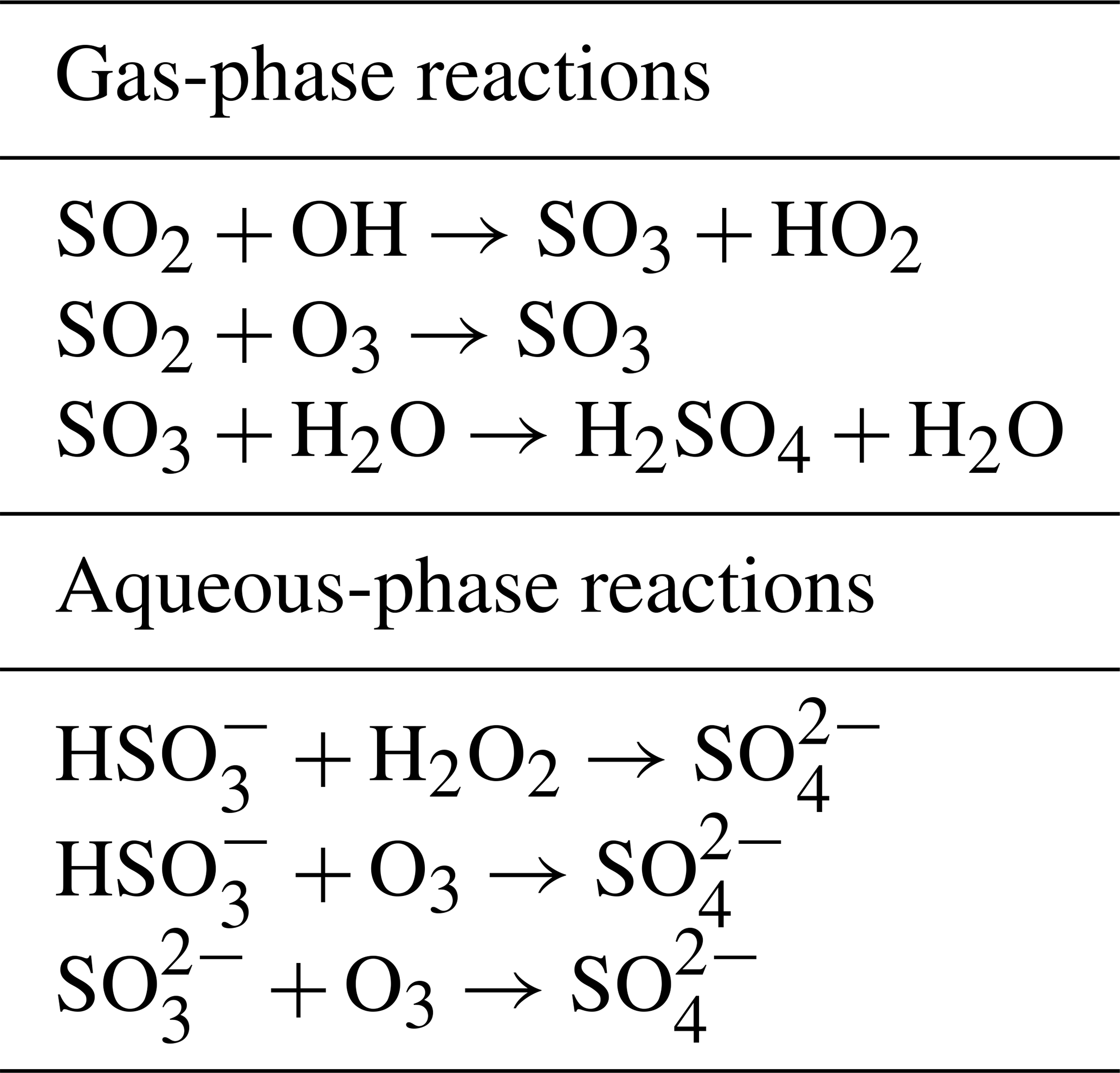
In the atmosphere SO2 can be oxidized in the gas phase by hydroxyl (OH) radicals and in the aqueous phase by reactions in cloud water and rainwater involving hydrogen peroxide (H2O2), ozone (O3), O2 catalyzed by transition metal ions, and other oxidants to form (see Turnock et al., 2019, and references within). The oxidation chemistry is necessarily simplified in many models due to the computational cost of detailed chemistry schemes, but studies have shown that oxidant levels can impact the lifetime of aerosol precursor species and ultimately global radiative forcing (Mulcahy et al., 2020; Karset et al., 2018). Uncertainty in aerosol radiative forcing also results from different values of cloud water pH, which alters formation by changing the rate of aqueous-phase oxidation of SO2 by ozone (Turnock et al., 2019). Observations have shown that cloud pH is both temporally and spatially variable (Aleksic et al., 2009; Murray et al., 2013; Schwab et al., 2016; Li et al., 2017), although measurements are very sparse. Typically, this variation is not accounted for in global chemistry climate models, including UKESM1 and its predecessor HadGEM3-GC3.1, both of which use a temporally and spatially constant cloud pH of 5.0. Turnock et al. (2019) found that increasing the cloud pH by 1.0 in HadGEM3-GC3.1 reduced the total SO2 column by up to 50 % over Europe, North America, and East Asia for 1970–1974 and 2005–2009. The impact on was variable due to the different SO2 loadings over the different regions and in the different time periods. Overall aerosol radiative forcings varied by up to 4 W m−2, with larger changes in some regions depending on whether cloud water pH was assumed to have increased or decreased over recent decades.
Loss of SO2 and to the Earth's surface by deposition can be through dry or wet processes. Dry deposition describes the removal of a gas or particle through direct contact of air with the Earth’s surface and wet deposition describes the incorporation of gases or particles into rain droplets or snow crystals and their subsequent removal through precipitation. Globally, dry deposition removes around 45 % of SO2 from the atmosphere (Chin et al., 2000). The importance of dry deposition in the global sulfur budget is the reason why we target it for development in UKESM1. Dry deposition of SO2 in ESMs is generally represented by a resistance in series approach (e.g. Archibald et al., 2020; Wu et al., 2020). Deposition of is mainly via wet processes (approximately 90 %, Chin et al., 2000), including nucleation scavenging within the cloud (rain out) and impact scavenging below the cloud (wash out), but dry deposition of does occur through gravitational settling. Deposition processes are necessarily parameterized in global models because they occur at sub-grid scales, and this contributes to model uncertainty. Further, observational flux data sets are sparse and frequently temporally and spatially limited, hindering model evaluation of deposition processes at regional to global scales.
Sulfur species are relatively well observed compared with many atmospheric components as their role in air pollution is well established. In the 1970s and 1980s the increasingly detrimental impacts of rising SO2 emissions on acid deposition, air quality, and human health in Europe and North America led to monitoring networks being set up in these regions (Tørseth et al., 2012; MACTEC-Engineering and Consulting, 2005). Rising pollution in Asia also led to the establishment of the Acid Deposition Monitoring Network in East Asia (EANET) in 2001 (e.g. Wang et al., 2008). However, even with these data sets it is only possible to evaluate model simulations of the recent historical period, and similar data sets are not available for other large source regions such as India, the Middle East, or remote regions. Further, the lack of a range of measurements, including flux observations, hinders detailed process studies at large scales. Since the early 2000s satellite observations of near-surface SO2 have also become available. Of these, the satellite data sets with the best temporal resolution and spatial coverage for SO2 are from the Ozone Monitoring Instrument aboard the NASA Earth-observing system Aura spacecraft (Fioletov et al., 2016). Although biases in the SO2 retrieval from OMI limit its use at high and low latitudes in winter and over areas with low atmospheric SO2 loading, they do provide valuable information over regions where there are no long-term or even any ground-based observations (Li et al., 2020; Levelt et al., 2018).
This paper is configured as follows: the model (UKESM1), the model simulations, observation data sets, and modifications to UKESM1's SO2 dry deposition parameterization are described in Sect. 2. In Sect. 3 we evaluate UKESM1 against observations of surface SO2 and and total column SO2. In Sect. 4 we assess the impact of the modifications to UKESM1's SO2 dry deposition parameterization. The discussion and conclusions are presented in Sects. 5 and 6.
2.1 UKESM1
UKESM1 is the latest-generation Earth system (ES) model developed in the UK. UKESM1 has HadGEM3-GC3.1 (Kuhlbrodt et al., 2018; Williams et al., 2018) as its physical–dynamical core. HadGEM3-GC3.1 is comprised of the Global Atmosphere 7.1 (GA7.1) configuration of the Unified Model (UM) (Walters et al., 2019; Mulcahy et al., 2018), the Nucleus for European Modelling of the Ocean (NEMO) model (Storkey et al., 2018), the Los Alamos Sea Ice Model (CICE, Ridley et al., 2018), and the Joint UK Land Environment Simulator (JULES) land surface model (Best et al., 2011). The additional ES process models include the stratospheric–tropospheric (StratTrop) version of the United Kingdom Chemistry and Aerosol (UKCA) model (Archibald et al., 2020), the Model of Ecosystem Dynamics, nutrient Utilisation, Sequestration and Acidification (MEDUSA, Yool et al., 2013), and the terrestrial biogeochemistry component of JULES (Clark et al., 2011). UKESM1 is described in detail, along with its component models and the coupling between them, by Sellar et al. (2019). The aerosol scheme used in UKESM1 (GLOMAP-Mode, Mann et al., 2010), including SO2 emissions and chemistry, is described in detail by Mulcahy et al. (2020). In UKESM1 the land and atmosphere share a regular latitude–longitude grid with a resolution of 1.25∘ × 1.875∘ (approximately 135 km at the mid latitudes). There are 85 vertical levels on a terrain-following hybrid height coordinate with a model lid at 85 km above sea level and 50 of these levels below 18 km. The ocean has a horizontal resolution of 1∘ and 75 vertical levels. While the atmospheric time step of the model physics is 20 min, due to the inherent computational cost of the chemistry and aerosol components, both of these components are called once per hour.
In UKESM1 the SO2 emissions including anthropogenic sources are from the CMIP6 inventory (Feng et al., 2020). Large explosive volcanic sources and biomass burning sources are not interactively modelled but are prescribed using the CMIP6 stratospheric aerosol climatology (Sellar et al., 2019) and van Marle et al. (2017) emission inventory respectively. Continuously degassing volcanic sources are also included as present-day, three-dimensional, temporally fixed (i.e. no seasonal variation) fields (Dentener et al., 2006). Emissions from the energy and industrial sectors are all emitted into the first model layer. We summarize how loss of SO2 from the atmosphere via oxidation and wet and dry deposition is modelled here, but for a detailed description of these processes in UKESM1 the reader is referred to Archibald et al. (2020) and Mulcahy et al. (2020). Gas- and aqueous-phase oxidation of SO2 to is represented by the reactions shown in Table 1 (Pham et al., 1996; Sander et al., 2003; Kreidenweis et al., 2003). Dry deposition of SO2 is parameterized following the resistance in series approach originally developed by Wesely (1989) (see Sect. 2.2.1). Loss via wet deposition is the SO2 that is scavenged and subsequently converted to in rainwater. It is parameterized as a first-order loss rate, calculated as a function of UKESM1's three-dimensional convective and large-scale precipitation (Archibald et al., 2020; O'Connor et al., 2014). Sulfate aerosol is also removed from the atmosphere by dry and wet deposition (Mulcahy et al., 2020). The aerosol dry deposition and sedimentation are represented by a resistance in series approach similar to that used for gaseous species but which also accounts for aerosol size (Mann et al., 2010). Wet deposition is parameterized in UKESM1 by an in-cloud convective plume-scavenging scheme following the approach described by Kipling et al. (2013) and by nucleation scavenging (Mulcahy et al., 2020).
2.2 SO2 dry deposition parameterization
The UKESM1 parameterization of SO2 dry deposition follows that described in Wesely (1989). This scheme uses the widely accepted approach of calculating the flux of a depositing gas as a function of a deposition velocity multiplied by the concentration gradient of the gas between a reference height (z, e.g. the lowest model level) and the receptor surface (Eq. 1). The deposition velocity is calculated by analogy with electrical resistance and is inversely proportional to three resistances to deposition, representing the three stages of gaseous transport to a receptor surface. These are (i) aerodynamic resistance (Ra) to gas transport through the near-surface turbulent layer, (ii) viscous resistance to gas transfer across a quasi-laminar layer surrounding the receptor surface (Rb), and (iii) structural resistance to deposition of the receptor surface itself (Rc). For a detailed description of this approach, see Wesely (1989), Erisman and Baldocchi (1994), and Zhang et al. (2003). The deposition velocity is calculated for each fractional surface type in a given model grid box, as is a resulting loss rate (flux) of SO2 from the atmosphere. The loss rates to each fractional surface are combined, resulting in the total loss of SO2 from the model atmosphere due to dry deposition. The deposition velocity is given by Eq. (2). If the surface is covered by vegetation, Ra is generally calculated at a zero-plane displacement height , where d is usually 0.6–0.8 times the vegetation height in metres. The UKESM1 calculations of Ra and Rb follow standard approaches (see Eqs. 3 and 4). The aerodynamic resistance, Ra, is calculated from the wind profile taking into account atmospheric stability and the surface roughness, where z0 is the roughness length, ψ is the Businger dimensionless stability function, κ is von Karman's constant, and u* is the friction velocity. The quasi-laminar sub-layer resistance, Rb, is calculated with Sc the Schmidt number and Pr the Prandtl number.
The surface or canopy resistance to deposition, Rc, is the most difficult of the three resistances to parameterize as it is sensitive to biochemical details of the individual receptor surfaces. Rc is typically a function of the following receptor-specific resistances: (i) canopy stomatal resistance (Rstom) combined with the mesophyll resistance (Rm) of a given plant, (ii) canopy cuticle or external leaf resistance (Rcut), and (iii) soil resistance (Rsoil), combined with an in-canopy resistance (Rinc), describing the turbulent transport of a gas through the plant foliage to the ground. The stomatal resistance, leaf cuticle resistance, and soil resistance are assumed to operate in parallel. For surfaces not covered with vegetation (e.g. open water, bare soil, or snow-covered surfaces), Rc is made equal to one of Rwater, Rsoil, and Rsnow. The receptor-specific resistances are combined as shown in Eq. (5) to calculate Rc. In UKESM1, Rstom follows the approach outlined in Wesely (1989), based on the original work of Baldocchi et al. (1987). Rstom is first calculated for water vapour for each vegetation type, and Rstom for other gases is then derived by scaling Rstom for water vapour by the ratio of the diffusion coefficient for the gas in question and that of water vapour. Due to a general lack of knowledge, Rm values are assumed to be zero for all gases. In UKESM1, Rinc and Rsoil are combined into a single value (referred to hereafter as Rsoil). In UKESM1, Rc for SO2 for the 13 fractional land cover types is initially set to the standard surface resistance (Rsurf) values given in Table A2.
2.2.1 Modifications to UKESM1's SO2 dry deposition parameterization
In this study we investigate two changes to the SO2 dry deposition parameterization in UKESM1. Firstly, we account for a key omission in UKESM1 in that for Rcut and Rsoil no account is taken as to whether the receptor surface is wet or dry nor of the near-surface relative humidity. Observational studies suggest that SO2 dry deposition (through a decrease in Rc) is significantly more efficient over wet surfaces compared with dry surfaces as well as for increasing values of near-surface relative humidity due to the high solubility of SO2 in water (e.g. Garland and Branson, 1977; Fowler, 1978; Erisman and Baldocchi, 1994; Erisman et al., 1994). We apply the findings from these studies to extend the calculation of Rcut for SO2 in UKESM1 to be a function both of whether the model vegetation is wet or dry and of the near-surface relative humidity. This change allows a surface to remain wet after rainfall for a period of 3 h, where previously it would have been “dry” immediately after the rainfall event. Rsoil for SO2 is also made a function of near-surface relative humidity. These changes are referred to as Rsurf-mod and will impact SO2 dry deposition over land surfaces. We include a more detailed description of the modifications to UKESM1's SO2 parameterization in Appendix A. Secondly, we change the surface resistance term for SO2 dry deposition to water (Rwater) from an erroneously high value of 148 to 1 s m−1 to better reflect the high solubility of SO2 in water. While lower than the value of 20 s m−1 used by Zhang et al. (2003), it reflects the small, observed value of 0.004 s m−1 from Garland (1977). This change is referred to as Rwater-mod and will impact SO2 dry deposition predominantly over the ocean.
In addition to the primary changes to the SO2 dry deposition parameterization (Rwater-mod and Rsurf-mod), we also include two secondary modifications. These are (1) an update in the calculation of the stability parameter () to better describe dry deposition under very stable atmospheric conditions and (2) a bug fix in the DMS chemistry. The stability parameter () describes the flux profile relationship and is important for calculating Ra in Eq. (3). Note that the Monin–Obukhov length (L) is derived locally in the UKCA code using local values of air density, temperature, and friction velocity, where the friction velocity is computed in the UM turbulence scheme and so is consistent across subroutines. Here we update the calculation of the stability parameter from that given by Dyer (1974) to that described by Holtslag and Bruin (1988). We also reduce the reference height for dry deposition (z) from 50 to 10 m. The reference height is the height below which there is no turbulence under very stable conditions and is also important for calculating Ra. Following Ganzeveld and Lelieveld (1995), the reference height should be half the average height of the lowest model layer, which in UKESM1 is 20 m. The changes to and z act to reduce the rate at which the deposition velocity decreases under very stable conditions, although we note that there is also an impact on the calculation of aerodynamic resistance under unstable conditions. The DMSO bug fix corrects the equation for DMS oxidation by OH (see Reaction R1) in UKCA's StratTrop mechanism, where the products incorrectly contain more sulfur atoms than the reactants. We substitute Reaction R1 with Reactions R2 and R3. This reduces the SO2 yield to a maximum of 0.84, which may be further reduced as DMSO deposits to the Earth's surface. However, the changes in simulated SO2 are actually only of the order of 1 % because anthropogenic sources are not affected by this change. Although the secondary changes incorporate important updates into the model, their impact on the atmospheric SO2 loading in UKESM1 is small in comparison to that driven by Rwater-mod and Rsurf-mod, and we do not discuss it here.
2.3 Model simulations
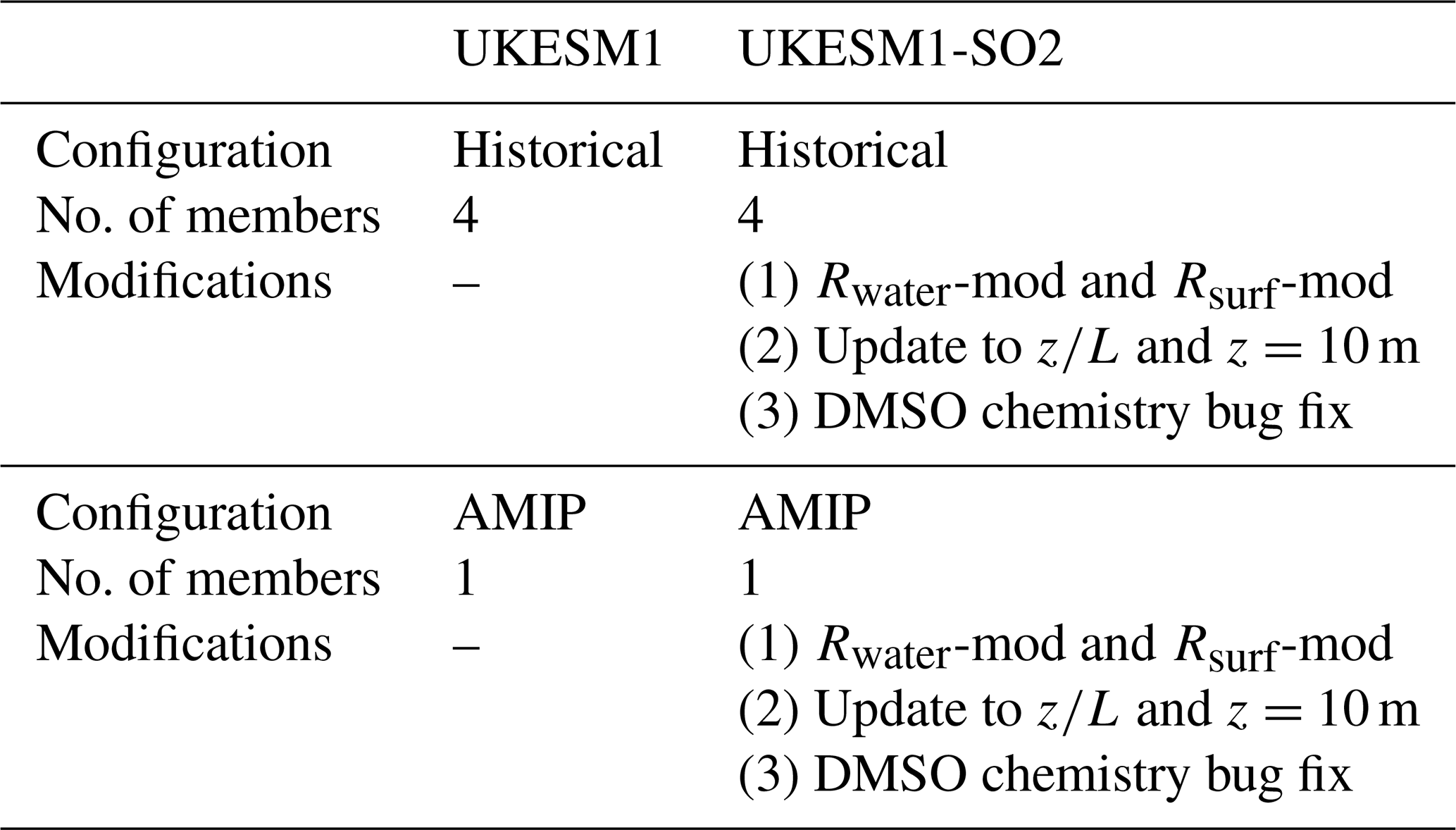
For this evaluation we initially use four simulations from the 19-member ensemble of historical simulations that were conducted for UKESM1's contribution to CMIP6 (Sellar et al., 2019; Tang et al., 2019). The historical simulations cover the period from 1850 to the end of 2014, thus modelling the evolution of climate and composition since the pre-industrial era. These simulations are forced by transient external forcings of solar variability, land use, well-mixed greenhouse gases, and other trace gas emissions and aerosols. The volcanic forcing due to the stratospheric injection of SO2 from volcanic eruptions is prescribed as a zonal mean climatology of the stratospheric aerosol optical properties over the historical period. All forcings and how they are implemented in UKESM1 are described fully in Sellar et al. (2019). Each historical ensemble member was initialized from a different date in the pre-industrial control simulation (Yool et al., 2020). We use monthly mean output for surface SO2 and concentrations and SO2 dry deposition flux. We use a second four-member ensemble of historical simulations to evaluate the impact of the changes to the SO2 dry deposition parameterization described in Sect. 2.2.1; hereafter, this ensemble is referred to as UKESM1-SO2. The UKESM1-SO2 historical simulations are set up and run as for the UKESM1 historical simulations. To calculate the detailed SO2 budget, we utilize the atmosphere-only configuration of UKESM1 and UKESM1-SO2. This is referred to as the Atmospheric Model Intercomparison Project (AMIP) configuration and allows us to generate the diagnostics required for the budget analysis that were not output in the historical simulations at a reduced computational cost. The UKESM1 AMIP configuration is driven by observed sea surface temperature (SST) and sea ice. It does not include the additional dynamic ocean and land surface components (Eyring et al., 2016). Instead, the required vegetation (vegetation fractions, leaf area index, canopy height) and surface ocean biology fields (DMS and chlorophyll) are taken from a single UKESM1 historical member and are prescribed as ancillary data, thereby maintaining traceability to the fully coupled model. For the SO2 budget calculations AMIP simulations were run from 1979 to the end of 1983.
2.4 Ground-based observations
We compare the modelled surface SO2 and concentrations to observations from the Clean Air Status and Trends Network (CASTNet, https://www.epa.gov/castnet, last access: 14 December 2021, Finkelstein et al., 2000) and the European Monitoring and Evaluation Program (EMEP, http://ebas.nilu.no/, last access: 14 December 2021; Tørseth et al., 2012). CASTNet provides surface observations of mean seasonal SO2 and concentrations which are available from 1987 to the present at 97 sites situated in the USA. In this study we used observations from the CASTNet sites designated as “western reference” or “eastern reference”. The reference sites have been reporting measurements since at least 1990 and are used for determining long-term trends (e.g. Clarke et al., 1997; Holland et al., 1998; MACTEC-Engineering and Consulting, 2005; Baumgardner et al., 2002). There are 16 western reference sites and 33 eastern reference sites which are located in the continental USA to the west and east of 100∘ W respectively (MACTEC-Engineering and Consulting, 2005). The eastern region is significantly more polluted than the western region due to the larger number of SO2 sources there. We therefore keep the western and eastern data sets separate to assess how UKESM1 performs in the two regions. Hereafter, we refer to the eastern and western USA regions as USA–E and USA–W respectively. For this evaluation we used the mean seasonal surface concentrations for SO2 and , which are measured with filter pack samplers at weekly sampling intervals. Details of the quality control procedures and of how the mean seasonal concentrations are calculated are given in Baumgardner et al. (2002).
We also evaluate simulated SO2 dry deposition flux from UKESM1 against observations from CASTNet, using the same eastern and western reference sites that were used to evaluate surface SO2 and concentrations. The CASTNet deposition fluxes are derived using modelled deposition velocities rather than directly measured fluxes, which are difficult to obtain due to the requirement for extensive instrumentation and technical resources. Direct measurements of SO2 dry deposition flux are therefore temporally and spatially limited and not suitable for evaluating long-term trends. To derive the SO2 dry deposition fluxes, measurements of SO2 concentration are combined with routine meteorological measurements, information on the land use type, and LAI at the measurement site. These data are then combined with modelled deposition velocities from the Multi Layer Model (MLM, Meyers et al., 1998; Saylor et al., 2014). The methodology used to derive the SO2 dry deposition fluxes for CASTNet is described in Clarke et al. (1997) and Baumgardner et al. (2002). While the modelled SO2 dry deposition fluxes can be under-predicted by approximately 30 % (Clarke et al., 1997), it is considered to be the best available approach to regional-scale assessment of dry deposition (Finkelstein et al., 2000; Baumgardner et al., 2002; Sickles and Shadwick, 2007a, b). This approach has been used to determine SO2 dry deposition fluxes for CASTNet since 1987 (e.g. Clarke et al., 1997; Baumgardner et al., 2002) and to assess global- and regional-scale models (Vet et al., 2014; Tan et al., 2018; Tang et al., 2018).
Surface SO2 and concentrations have been monitored at EMEP sites for the period 1972–present (Tørseth et al., 2012). In this study we have used observations of surface concentrations of SO2 and from 48 and 42 sites respectively. We have selected sites where there are at least 10 years of continuous measurements and with a few exceptions have used sites where SO2 and were co-located. We use monthly mean observations for both species. No SO2 dry deposition data were available from EMEP. The locations of the CASTNet and EMEP sites used in this study are shown in Fig. 1.
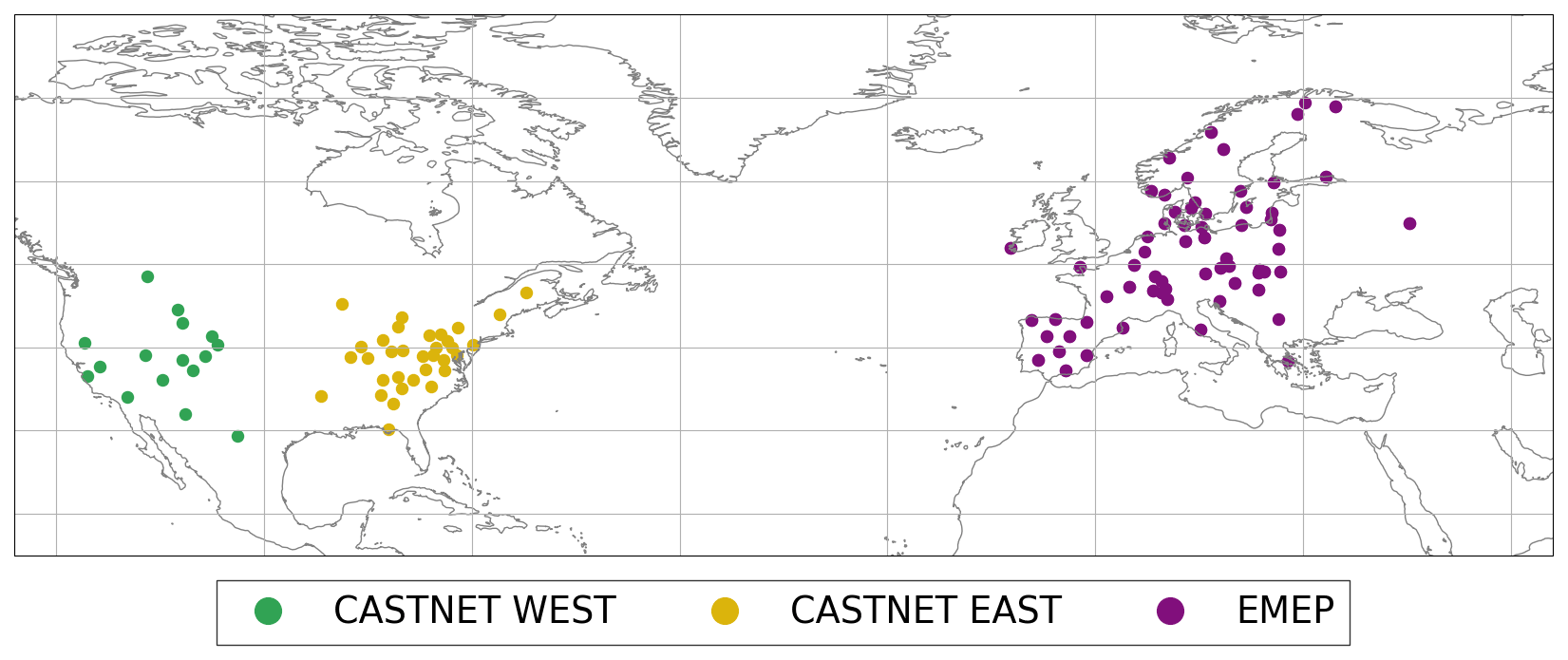
Figure 1Map of the locations of the CASTNet and EMEP measurement sites used in this study.
2.5 Data processing
For this evaluation we calculated seasonal averages for the modelled surface SO2 and concentrations and for the EMEP observational data. The seasonal periods were defined as December–January–February (DJF), March–April–May (MAM), June–July–August (JJA), and September–October–November (SON). The CASTNet data for all variables were available as seasonal averages for these periods. Model grid cell output was co-located with the CASTNet and EMEP measurement sites. In some cases, this resulted in model data from a particular grid cell being compared with more than one measurement site. For the time series analysis, regional means and standard deviations were calculated across the sites in the USA–E, USA–W, and Europe regions. Although there is spatial variation in the surface SO2 and concentrations across Europe, for example concentrations are relatively low in Scandinavia but are much higher in south-eastern Europe, it is less easy to classify “clean” and “polluted” regions at the global model scale. Therefore we classify Europe as a single region. For the spatial analysis and calculation of time series statistics, we calculate mean values over the whole time series, i.e. 1987–2014 and for two time slices at the start (1990–1995) and end of the time series (2009–2014). For the time slices we only used sites that had at least 3 out of 5 years of data available. We investigate the two time slices to assess the model's performance during the different pollution levels at the start and end of the time series. We determine the rate of change (trend) in the surface concentrations by calculating the linear regression for 1987–2014, 1990–1995, and 2009–2014.
2.6 Satellite observations
Total column SO2 (TCSO2) measurements came from the Ozone Monitoring Instrument (OMI) and were obtained from the Goddard Earth Sciences Data and Information Services Centre (https://aura.gesdisc.eosdis.nasa.gov/data/Aura_OMI_Level2/OMSO2.003, last access: 14 December 2021) (Li et al., 2020). OMI is situated on board NASA's polar-orbiting Aura satellite launched in 2004 with a local overpass time of approximately 13:45 local solar time (LST). OMI has a nadir footprint of 13 km × 24 km and a spectral viewing range of 270 to 500 nm (Levelt et al., 2018). The TCSO2 product is quality controlled for cloud radiation fraction > 0.0 and < 0.5, solar zenith angle < 65∘, the South Atlantic Anomaly flag = 0, ice cover flag = 0, the air mass factor (AMF) > 0.3, and TCSO2 > −1.0 Dobson unit (DU). Background TCSO2 average values tend to be positive near-zero quantities (i.e. just above 0.0), where some soundings are slightly negative. If only positive TCSO2 were incorporated into the background averages, this would positively skew the true value.
For a robust comparison between model simulations and satellite data, both data sets typically require spatiotemporal co-location to reduce sampling (representation) errors. To achieve this, high temporal resolution (e.g. 3-hourly or 6-hourly) model outputs of three-dimensional tracer and pressure fields are required over the analysis period to capture e.g. diurnal variability (Pope et al., 2016; Monks et al., 2017). However, this is difficult when using standard climate model simulations, including those used in this study, which typically output monthly means due to their long-term climate focus. In this comparison we performed tests to show that using the monthly mean model output was suitable given the relatively uniform diurnal cycle of SO2 emissions. For these tests we made initial comparisons of model output and satellite data using 6-hourly and monthly mean output from the same UKESM1 simulation. We found that the temporal sampling of the model was not overly critical for SO2, i.e. that modelled SO2 has a sufficiently long lifetime to dampen the influence of diurnal sampling of the model. Further details on the TCSO2 product, how it was processed to obtain TCSO2 values, and the assessment of the temporal resolution are given in Pope and Chipperfield (2021).
3.1 Time series analysis of surface concentrations of SO2 and
UKESM1 simulations of surfaces of SO2 and concentrations are compared with observations from the CASTNet and EMEP networks for the period 1987–2014 in Fig. 2. The statistics summarizing the model bias and trends over this period as well as for the 1990–1995 and 2009–2014 time slices are shown in Tables 3 and 4. We find that UKESM1 captures the historical reduction in surface SO2 and concentrations. This is in agreement with Aas et al. (2019), who reported that an ensemble of global aerosol models was generally able to capture the recent historical declines in these two species over the USA and Europe. UKESM1 over-predicts surface SO2 concentrations in all three regions, but the direction of the model's bias in surface concentrations is spatially variable.
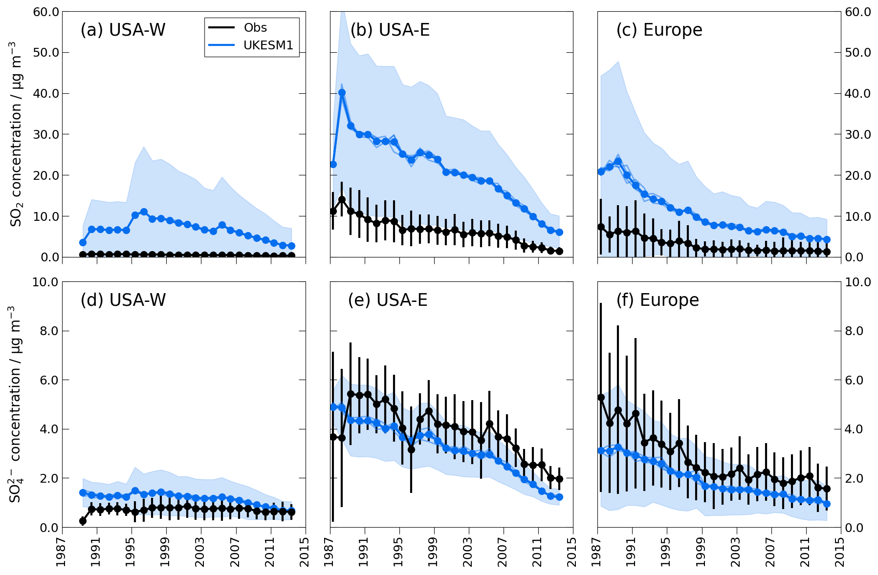
Figure 2Time series of observed and modelled mean annual surface SO2 (a–c) and (d–f) concentrations for USA–W (a, d; N sites = 16), USA–E (b, e; N sites = 33), and Europe (c, f; N sites = 48 for SO2 and 42 for ). Each point in the time series represents the mean across the measurement sites in the region. Note that the vertical scale for SO2 (a–c) is a factor of 6 larger than that for (d–f).
Figure 2a–c show that in both Europe and USA–E the model over-predicts surface SO2 concentrations, particularly at the start of the time series, which then decrease too rapidly. Over Europe, the observed surface SO2 concentrations decrease at a rate of 0.72 µg m−3 yr−1 in the period 1990–1995 which slows to 0.38 µg m−3 yr−1 by 2009–2014. However, the modelled surface SO2 concentrations decrease by 2.52 µg m−3 yr−1 for 1990–1995, slowing to only 1.31 µg m−3 yr−1 by 2009–2014. Over USA–E the observed surface SO2 concentrations decrease at similar rates at the start and end of the time series. UKESM1 is better able to capture the trend at the start of the time series but simulates an overly rapid reduction in surface SO2 concentrations after 2005 (see Fig. 2b). Over USA–E UKESM1 simulates the sharp drop in surface SO2 concentrations that occurred in 1995 following the implementation of Phase 1 of the USA's Clean Air Act Amendments (McHale et al., 2021). However, the model then simulates relatively high surface SO2 concentrations for the period 1996–1999 rather than the sustained lower surface SO2 concentrations that are observed after 1995. Over USA–W the observed surface SO2 concentrations remain steady from 1987 to 2014 due to there being fewer sources in this region. Figure 2a shows that UKESM1 simulates the steady surface SO2 concentrations at the start of the time series, albeit with a positive bias. However, after 1995 UKESM1 simulates decreasing surface SO2 concentrations in USA–W, which brings the modelled values into better agreement with the observations but introduces an artificial trend into the modelled time series.
UKESM1 over-predicts the annual mean surface SO2 concentrations in the polluted regions of Europe and USA–E by a factor of 3.2 to 3.4 over the period 1987–2014, although the absolute bias is higher USA–E (see Table 3). While the absolute magnitude of the bias in mean annual surface SO2 concentration is less in USA–W compared with the polluted regions, proportionally it is much larger, with the model simulating surface SO2 concentrations by more than 10 times the observed values. The absolute magnitude of the bias in mean annual surface SO2 concentration decreased from 1990–1995 to 2009–2014 in all three regions (see Table 3), reflecting the model's more rapid decrease in surface SO2 concentrations relative to the observations. However, the normalized mean bias (NMB) values were slightly higher in 2009–2014 compared with 1990–1995.
Table 3Statistics for mean annual surface SO2 concentrations at USA–W, USA–E, and Europe. The mean and trend values are in µg m−3 and µg m−3 yr−1 respectively.

Table 4Statistics for mean annual surface concentrations at USA–W, USA–E, and Europe. The mean and trend values are in µg m−3 and µg m−3 yr−1 respectively.
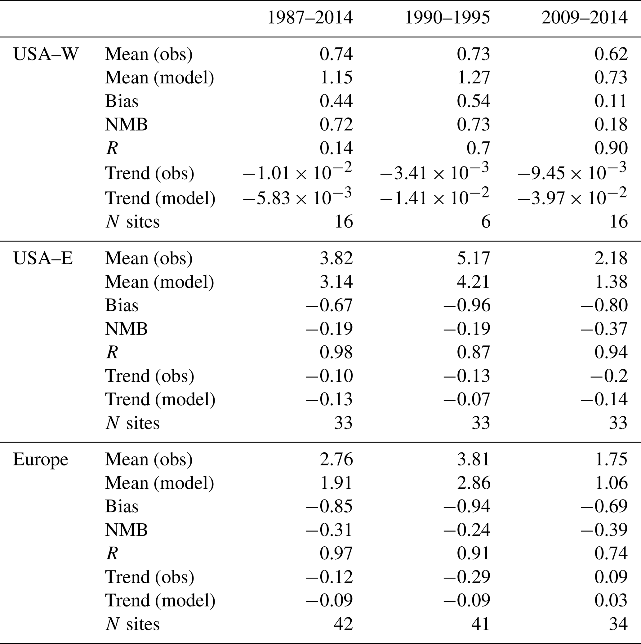
Figures 2e–f show that UKESM1 captures both the magnitude and trends in surface concentrations better than the surface SO2 concentrations. The model simulated surface concentrations decreasing at a rate of 0.13 µg m−3 yr−1 (USA–E) and 0.09 µg m−3 yr−1 (Europe) compared with the observed trend of ≈0.10 µg m−3 yr−1 (see Table 4). UKESM1 does under-predict mean annual surface concentrations in the polluted regions of USA–E and Europe, but the model bias is relatively small compared with the large over-prediction of mean annual surface SO2 concentration (see Tables 3 and 4). We also find that there is a large range associated with the modelled and observed data and that the mean surface concentrations lie within these ranges. The model bias remained relatively constant over the period from 1987 to 2014, ranging from −0.96 to −0.80 µg m−3 for the periods 1990–1995 and 2009–2014 over USA–E and from −0.91 to −0.69 µg m−3 for the same periods over Europe (see Table 4). The picture is different in USA–W, where, in contrast to USA–E and Europe, UKESM1 over-predicts mean annual surface concentration by an average of 150 % for 1987–2014. Both the absolute model bias and the NMB are worse in 1990–1995 than in 2009–2014, which may be attributed to the model simulating a much faster decrease in mean annual surface concentrations compared with the observed trend for the later period (see Table 4).
3.2 Spatial evaluation of surface SO2 and concentrations
Figures 3 and 4 show the spatial distribution of modelled and observed mean annual surface SO2 and concentrations for the periods 1990–1995 and 2009–2014 for the USA and Europe. We find that UKESM1 captures the spatial distribution of surface SO2 and concentrations over each region, simulating higher concentrations in USA–E, central Europe, and eastern Europe, where there are numerous large sources, and lower concentrations in USA–W and northern Europe, which have far fewer sources (see Fig. B1). These figures also show the localized versus dispersed nature of the surface SO2 and concentrations, with high SO2 concentrations located within two to three grid boxes (200–400 km) of the emission sources (see Fig. B1), while is distributed more widely. Figure 3 shows that modelled and observed surface SO2 and concentrations across the USA are lower in 2009–2014 compared with 1990–1995, demonstrating the widespread impact of emission reduction policies. However, the disparity between higher concentrations in USA–E and lower concentrations in USA–W is still apparent for both species in the later period.
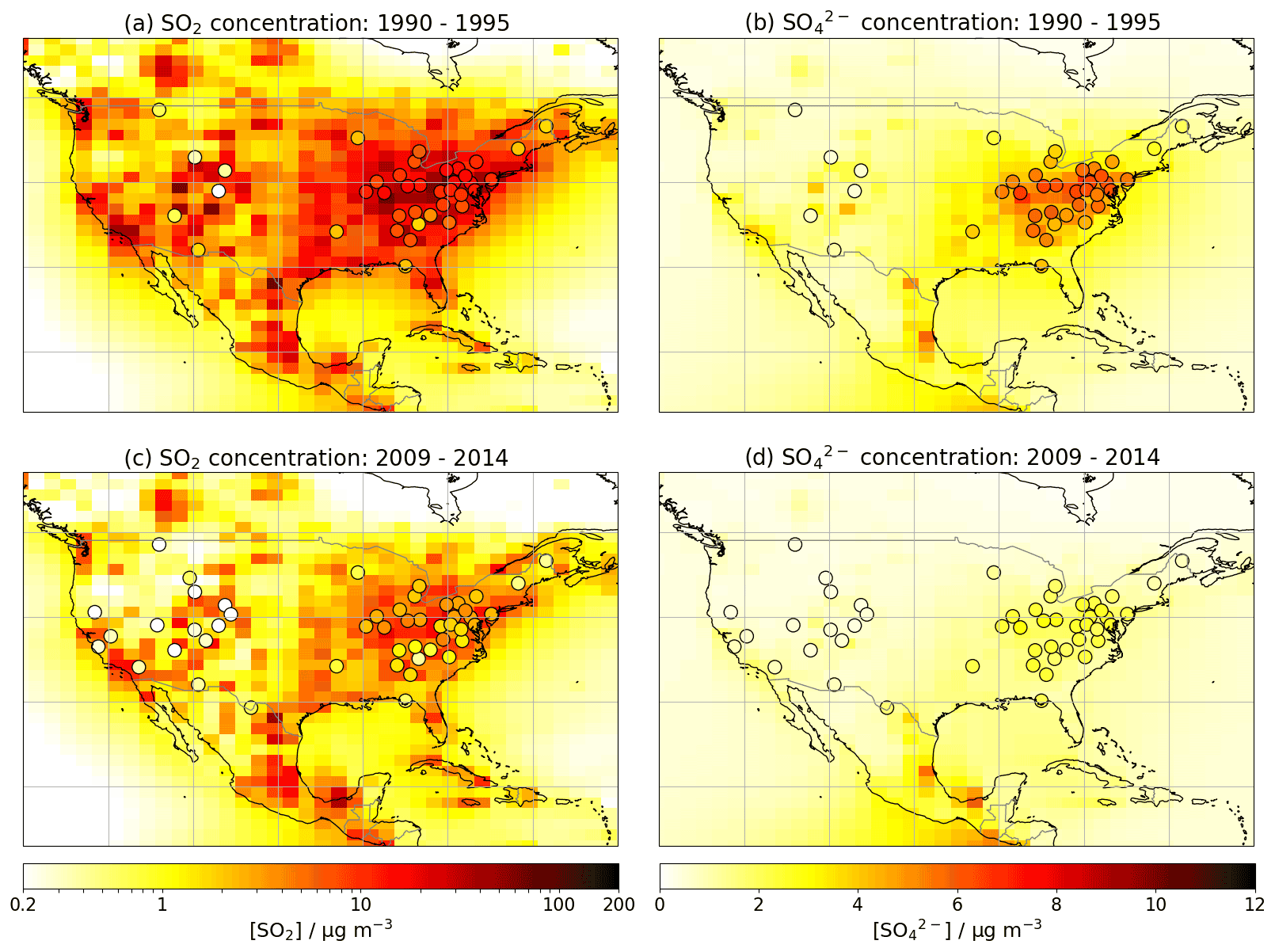
Figure 3Mean annual surface SO2 concentration (a, c) and surface concentration (b, d) for 1990–1995 (a, b) and 2009–2014 (c, d) for modelled output. Observations from 49 CASTNet measurement sites are plotted as black-edged circles on the same colour scale.

Figure 4Mean annual surface SO2 concentration (a, c) and surface concentration (b, d) for 1990–1995 (a, b) and 2009–2014 (c, d) for modelled output. Observations from EMEP measurement sites (N sites = 48 for SO2 and 42 for ) are plotted as black-edged circles on the same colour scale.
In Europe the highest mean annual surface SO2 and concentrations were observed in central and eastern Europe and the south-east (SE) of England (see Fig. 4). Lower concentrations of both species were observed in northern and western regions, e.g. Scandinavia and the western coast of Ireland. Figure 4c shows that mean annual surface SO2 concentrations were generally lower in 2009–2014 compared with 1990–1995, especially in central and eastern Europe, due to the impact of air quality legislation. However, for 2009–2014 modelled and observed levels of SO2 remain high in the south-eastern region (see Fig. 4c). UKESM1 reproduces the spatial distribution of mean annual SO2 concentrations across Europe but has large positive biases over most of the region. The largest model biases were in eastern and south-eastern Europe during the period 1990–1995, where UKESM1 simulates mean annual surface SO2 concentrations of up to 100 µg m−3 compared with observed values of 10–30 µg m−3. Figure 4b shows that UKESM1 captures the spatial distribution between low mean annual surface concentrations in northern and western regions of Europe and high mean annual surface concentrations in central Europe. However, the model under-predicts mean annual surface concentrations at many locations across Europe, with the largest biases occurring across Denmark and the regions surrounding the Baltic Sea.
3.3 Spatial distribution of model bias in surface SO2 and concentrations
Figures 5 and 6 show that the direction of the model biases, whether positive or negative, is generally consistent across a region. UKESM1 over-predicts mean annual surface SO2 concentration for all sites in both the USA–E and USA–W regions and, with the exception of some Scandinavian sites, across Europe. Figures 5 and 6 also show that mean annual surface concentrations are generally under-predicted across the USA–E and European sites while being over-predicted at the USA–W sites.

Figure 5Geographic distribution of mean bias (UKESM1 – obs) in mean annual surface SO2 and concentration at 49 CASTNet measurement sites. The mean annual surface concentrations are calculated over the period 1987 to 2014. Absolute mean bias (MB) is shown in (a) and (b) and normalized mean bias (NMB) is shown in (c) and (d). Note that different scales are used for the SO2 model bias (a) and normalized mean bias (c).
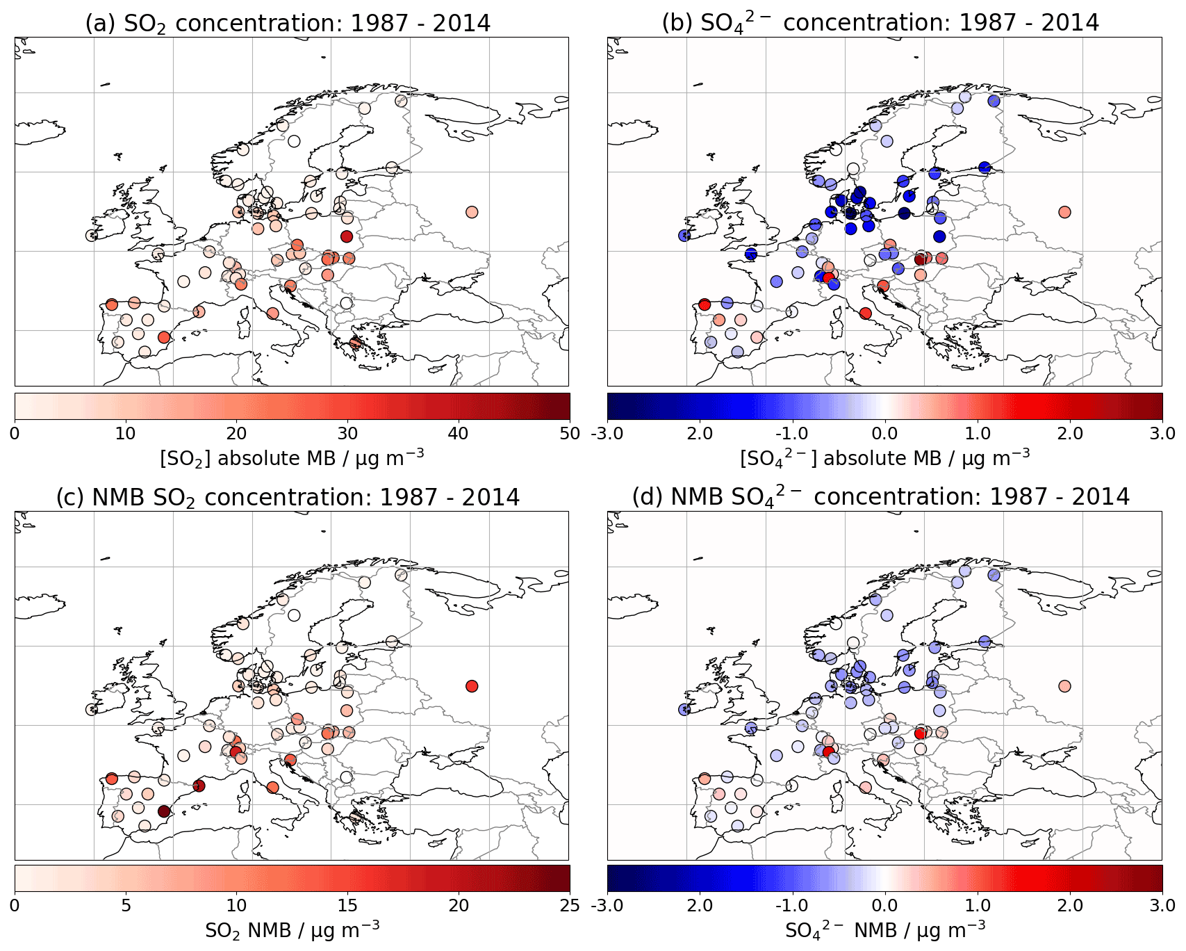
Figure 6Geographic distribution of mean bias (UKESM1 – obs) in mean annual surface SO2 and concentration at EMEP measurement sites (N sites = 48 for SO2 and 42 for ). The mean annual surface concentrations are calculated over the period 1987 to 2014. Absolute mean bias is shown in (a) and (b) and NMB is shown in (c) and (d). Note that different scales are used for the SO2 model bias (a) and normalized mean bias (c).
The model's over-prediction of mean annual surface SO2 concentration is largest close to the sources. For example, UKESM1 over-predicts surface SO2 concentrations by up to 50 µg m−3 in the central USA–E area but only by around 10 µg m−3 at the surrounding sites, whilst in Europe the largest biases of around 10–20 µg m−3 tend to be in central and eastern areas. The model's tendency to over-predict SO2 concentrations to a greater extent close to the sources is also shown in the plots of NMB (see Figs. 5c and 6c) and is likely why there is a larger range in the modelled mean annual surface SO2 concentrations averaged across the USA–E and European measurement sites compared with the observational values (see Fig. 2b and c). Figures 5b and 6b show that UKESM1 generally under-predicts surface concentration across the USA–E and European sites, with model biases of −1 to −3 µg m−3. We find that in USA–E the largest negative biases in surface concentrations are not necessarily co-located with the largest positive biases in SO2, instead occurring at sites several hundred kilometres from the large point sources. Similarly, in Europe the largest biases in surface concentrations occur further north than the large biases in surface SO2 concentration, and at certain sites located near large sources, UKESM1 over-predicts surface concentrations. The plots of NMB show that there is less spatial variation in the model bias for surface concentrations, reflecting UKESM1's ability to capture the more distributed nature of atmospheric . In USA–W UKESM1 over-predicts both SO2 and concentrations at almost all of the sites (see Fig. 5). For SO2 this is a consequence of the sparsely distributed measurement sites being located in rural regions remote from any of the sources in USA–W (Clarke et al., 1997; MACTEC-Engineering and Consulting, 2005; Baumgardner et al., 2002) (see also Fig. B1). This results in some very large NMB values in USA–W (see Fig. 5a).
3.4 Seasonal cycles
Figure 7 shows modelled and observed surface SO2 and concentrations averaged seasonally for the period 1987–2014. The comparison between the model and observations is summarized for DJF and JJA in Table 5. The higher wintertime SO2 concentrations are driven by greater emissions from coal-fired power plants and domestic heating and less oxidation. Conversely, there are fewer emissions and higher oxidant concentrations in summertime. These cycles drive correspondingly low concentrations in winter and high concentrations in summer. Overall, we find that the model bias in surface SO2 and concentrations depends on the season as well as the region and pollution levels.
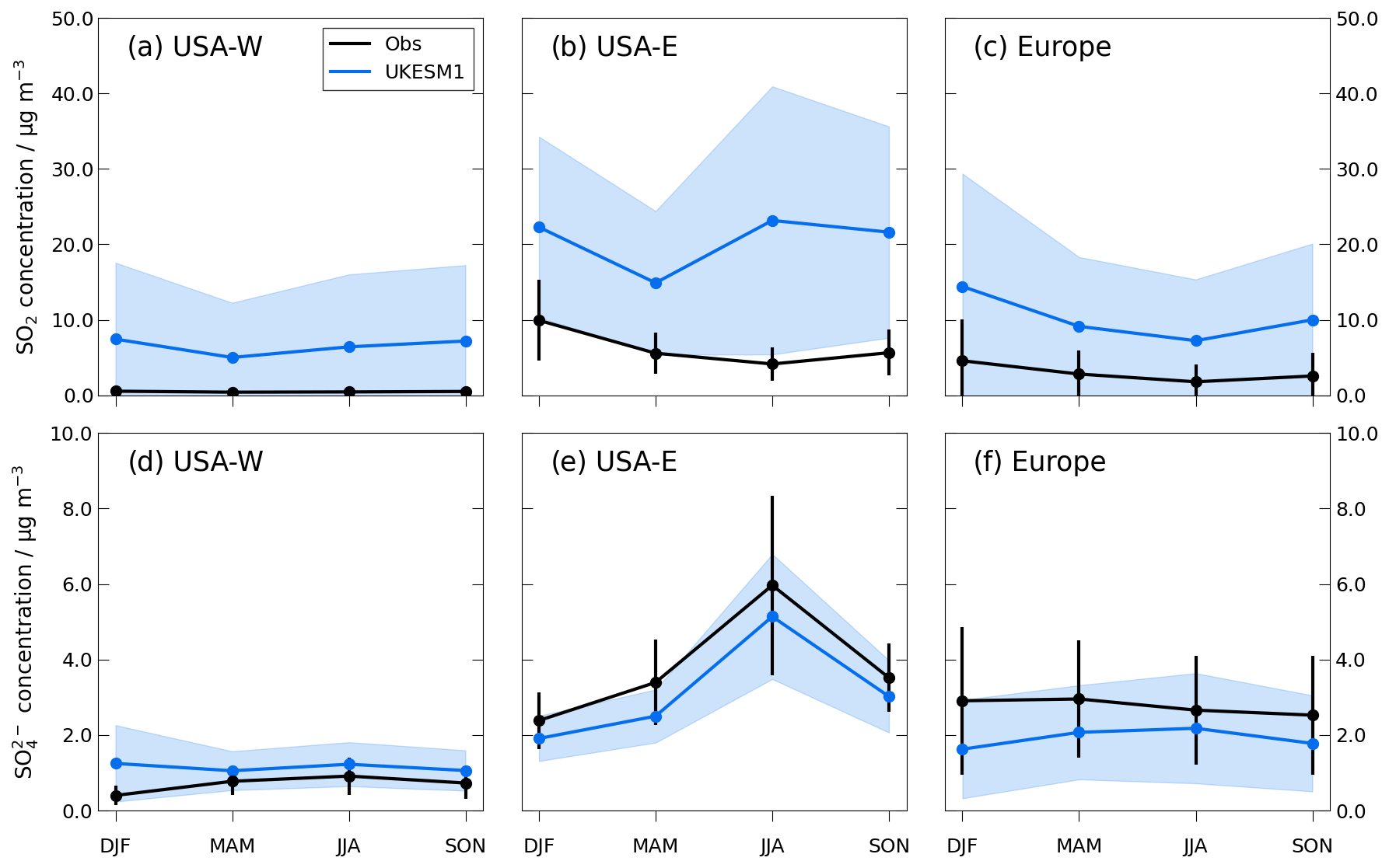
Figure 7Modelled and observed seasonal mean surface SO2 concentration (a–c) and surface concentration (d–f) for the period 1987–2014. USA–W (a, d; N sites = 16); USA–E (b, e, N sites = 33), and EMEP (c, e; N sites (SO2) = 48 and N sites () = 42). The blue-shaded region and the black error bars represent the standard deviation across the sites in the observational network.
Table 5Statistics for seasonal mean surface SO2 and concentrations (µg m−3) at USA–W, USA–E, and Europe. The mean seasonal values are averaged over the period 1987–2014.
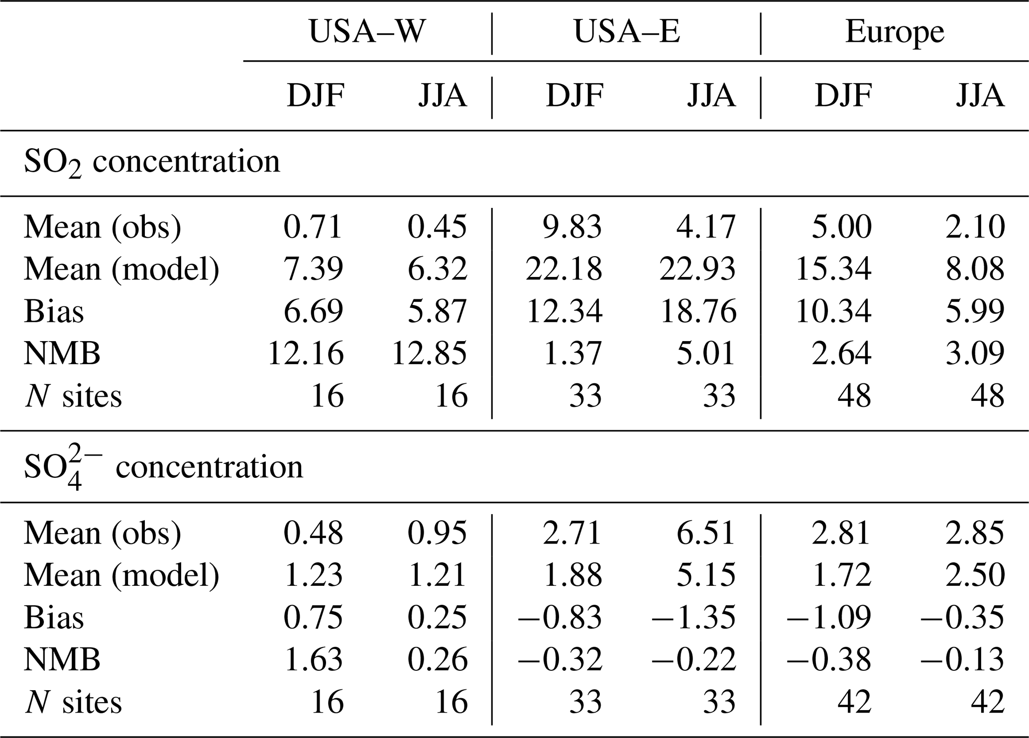
The results presented in Sect. 3.1 and 3.2 show that UKESM1 consistently over-predicts mean annual surface SO2 concentrations in the USA and Europe. However, Fig. 7a–c show that in the more polluted regions (USA–E and Europe), the magnitude of the bias is seasonal although still with a large positive bias. UKESM1 is able to capture the seasonal cycle in surface SO2 concentrations over Europe, but the absolute model bias is larger in DJF compared with JJA (see Table 5). In USA–E UKESM1 does not capture the seasonal cycle in surface SO2 concentrations due to the relatively large model bias in JJA, where the modelled SO2 concentrations are over 5 times the observed values. In USA–W the modelled and observed surface SO2 concentrations are slightly higher in DJF compared with JJA, but the model bias is so large in this region that it is difficult to determine whether there is any seasonality in this bias.
UKESM1 clearly captures the seasonal cycle in surface concentration over USA–E, simulating the highest values in summer and the lowest values in winter. The model under-predicts surface concentration by a factor of 0.7 to 0.8 reasonably consistently throughout the seasonal cycle. In the cleaner USA–W region, UKESM1 is able to capture the seasonal cycle in surface concentrations, with the exception of DJF, where the model over-predicts surface concentrations by a factor of 2.5. In Europe the observed seasonal cycle in surface concentration has only a small amplitude, with mean values of 2.81 and 2.85 µg m−3 in DJF and JJA respectively.
3.5 Evaluation of total column SO2 in UKESM1 against satellite observations
Figure 8 shows total column SO2 (TCSO2) from UKESM1 and OMI and the difference between them for DJF and JJA. Note that the quality control for solar zenith angle results in no data availability above 65∘ N or below 65∘ S in the winter months, and due to OMI's weaker sensitivity to retrieving SO2 in remote regions, we focus on comparing TCSO2 over source and outflow regions (Li et al., 2020). Figure 8a–d show that UKESM1 and OMI broadly agree on the location of the main Northern Hemisphere (NH) source regions, including China, India, Europe, and the USA. The model and satellite data both show seasonal cycles in TCSO2 over the large source regions, with higher values being modelled and observed during the winter months. However, Fig. 8e and f show that the UKESM1 TCSO2 values were generally larger than the OMI TCSO2 values in these source regions by 0.6–1.0 DU. Over the background regions UKESM1 over-predicts TCSO2 values by 0.2–0.5 DU. UKESM1 also has larger volcanic sources and associated outflow, which can be seen over central America, Sicily, Hawaii, and Papua New Guinea, for example. This is likely due to the climatology that UKESM1 uses for continuously degassing volcanoes. In agreement with the ground-based observations, the satellite data show an east–west divide in the USA, with greater TCSO2 over USA–E compared with USA–W.
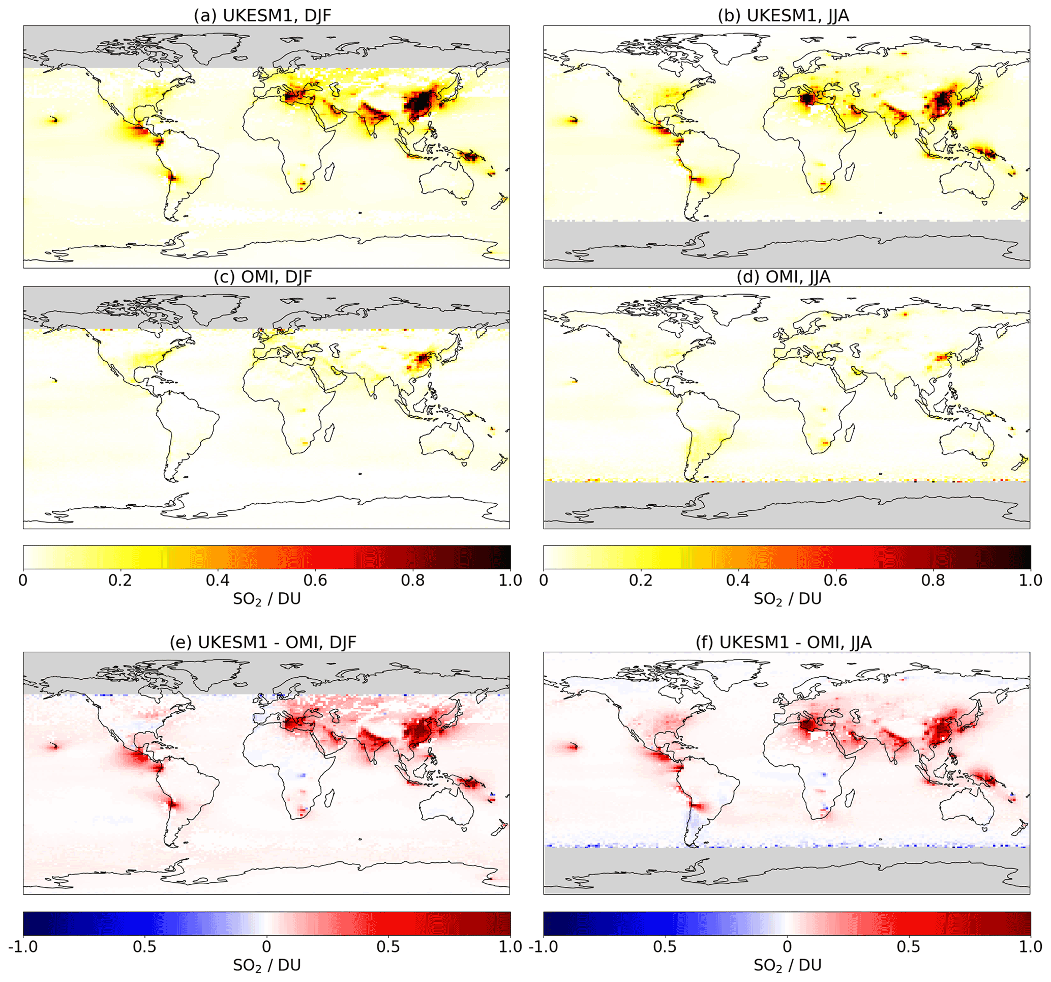
Figure 8Total column SO2 for UKESM1 (a, b), OMI (c, d), and UKESM1 – OMI (e, f). DJF is shown in the left column and JJA is shown in the right column. Median total column SO2 in Dobson units is calculated for the period 2005–2014.
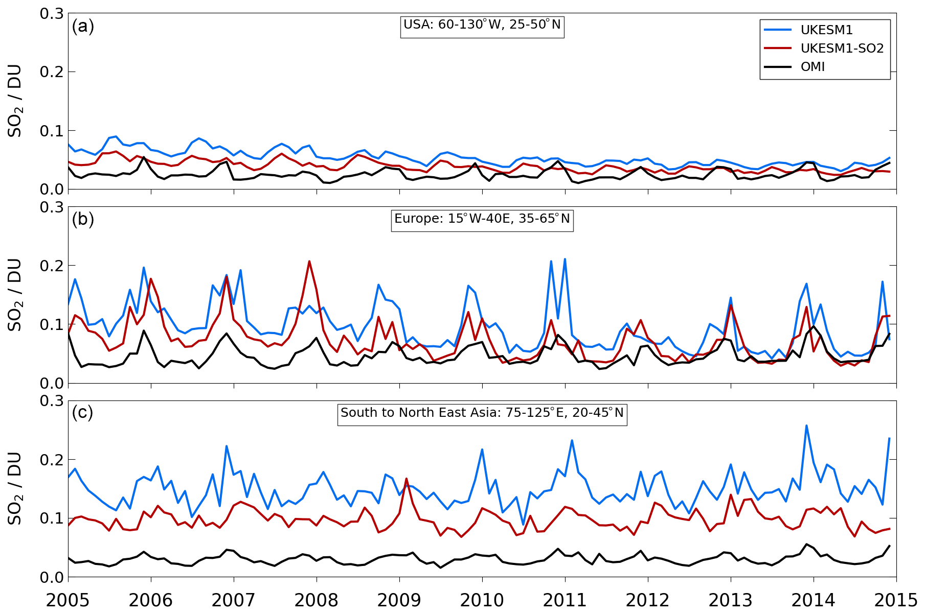
Figure 9Median total column SO2 calculated for 2005–2014 for USA (a), Europe (b), and South to North-east Asia (c). Total column SO2 is in Dobson units.
Table 6Statistics comparing model and OMI total column SO2 over three regions: USA (60–130∘ W, 25–50∘ N), Europe (15∘ W–40∘ E, 35–65∘ N), and South to North-east Asia (75–125∘ W, 20–45∘ N) for the period 2005–2014. The metrics are mean bias (MB, DU), root mean square error (RMSE, DU), percentage mean bias (MB %), and correlation (R).
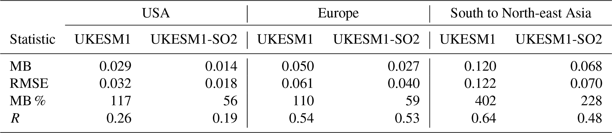
Note that the median value is reported for each metric.
Figure 9 shows modelled and observed TCSO2 over the period from 2005 to 2014 for three source regions, the USA (60–30∘ W, 25–50∘ N), Europe (15–40∘ E, 35–65∘ N), and South to North-east (SNE) Asia (75–125∘ E, 20–45∘ N). Overall, we find that the observed TCSO2 is reasonably stable over this period in all three regions and that there are clear seasonal cycles showing peak TCSO2 during the NH winter in the USA and Europe and slightly earlier ones in SNE Asia. However, Fig. 9a and b show that modelled TCSO2 decreases over the USA and Europe from 2005 to 2010, with UKESM1 over-predicting TCSO2 by up to 0.1 DU at the start of the time series. After 2011, UKESM1 is in much better agreement with the observed TCSO2 over both regions. Figure 9c shows that UKESM1 consistently over-predicts TCSO2 over SNE Asia by 1.5–2.0 DU during the period from 2005 to 2014. UKESM1 does simulate a seasonal cycle in TCSO2 in all three regions. In Europe, UKESM1 is able to predict the peak wintertime TCSO2 values, although between 2005 and 2010 the model has a positive bias of up to 0.1 DU. However, in the USA and to a lesser extent in SNE Asia (Fig. 9a and c respectively), UKESM1 mistimes the peak TCSO2 values. In the USA the model simulates the highest values in the summer rather than in winter, and in SNE Asia the modelled peak TCSO2 values appear shifted by several months earlier relative to the observations.
The observations of TCSO2 and surface SO2 concentrations over Europe both show the impact of emission control policies on keeping atmospheric SO2 levels low (Figs. 2c and 9b). However, for the USA, we investigate the surface SO2 concentrations separately over the USA–E and USA–W regions, whereas the TCSO2 is averaged over the continental USA as a whole. As a result, TCSO2 does not appear to decrease over the period 2005–2014 in the same way surface SO2 concentrations are reduced in USA–E (Figs. 2b and 9a). Using a mean TCSO2 for the continental USA as a whole also results in lower values relative to Europe. This is in contrast to the ground-based observations, where surface SO2 concentrations over Europe are intermediate between USA–E and USA–W for the period 2005–2014. The relatively high TCSO2 over Europe is also due to the inclusion of a number of large eastern European sources which are not well represented in the ground-based observations. We find that the TCSO2 and surface SO2 concentration observations both agree on the seasonal cycle, showing higher values in winter compared with the summer.
UKESM1 over-predicts surface SO2 concentration to a greater extent than TCSO2 for the USA and Europe. The model over-predicts surface SO2 concentration by factors of 2.2–11.6 for USA–E and USA–W and 2.4 for Europe compared with values of 1.2 (USA) and 1.1 (Europe) for modelled TCSO2 (see Tables 3 and 6). However, the R values for surface SO2 concentration (>0.8) are much better than those for TCSO2 (0.26–0.53), particularly over the USA. The low R value for the USA reflects the poor seasonal agreement in TCSO2 in this region. The comparison against both observational data sets shows that the modelled atmospheric SO2 is too high, both at the surface and through the column. In addition, UKESM1 simulates larger trends in TCSO2 and surface SO2, particularly prior to 2010, than are seen in the observations. Both observational data sets also show that UKESM1's over-prediction of atmospheric SO2 in the large source regions is generally greater in the winter months compared with the summer months (see Fig. 8e and f). Exceptions occur in USA–E, where UKESM1 fails to capture the seasonal cycle in atmospheric SO2, over-predicting surface SO2 concentration and TCSO2 to a greater extent in JJA compared with DJF. Notably, in the southern USA–E region and the Iberian Peninsula, UKESM1 actually under-predicts TCSO2 by up to 0.1 DU in DJF, which does not occur in the comparison with surface SO2 concentrations, even if the model and observations are compared at individual CASTNet and EMEP sites.
4.1 Global-scale impacts
Figure 10 shows SO2 dry deposition velocity simulated by UKESM1 and how this is affected by changes to the SO2 dry deposition parameterization. In UKESM1 the mean annual deposition velocities range from approximately to m s−1 (see Fig. 10a). Figure 10b, e, and h show that SO2 dry deposition velocity increases over almost all land and ocean regions in UKESM1-SO2 by approximately 0.02–0.08 m s−1. This represents an increase of a factor of 2–4 relative to UKESM1. The largest increase in SO2 dry deposition velocity to the ocean is over the Southern Ocean in winter, where it increases by more than a factor of 4 (see Fig. 10i). Over land surfaces the largest increases occur over South America, north-western America and Canada, and north-eastern Europe/western Russia (see Fig. 10f and i). The increased SO2 dry deposition velocities in UKESM1-SO2 relative to UKESM1 indicate that the changes to the SO2 dry deposition parameterization are behaving as expected. The reduction in Rc for SO2 dry deposition to water increases the dry deposition velocity to oceans. Similarly, when land surfaces are allowed to remain wet for a longer period after rainfall events, Rcut and Rsoil are reduced for a longer period of time in UKESM1-SO2 relative to UKESM1 and SO2 dry deposition velocity to the canopy (leaf or soil) increases. In the summer months SO2 dry deposition velocities are larger over land surfaces compared with in the winter months, while over oceans values are larger in the winter compared with the summer. Although increased rainfall in winter drives wetter surface conditions, the leaf canopy is reduced or absent, and at high latitudes surfaces are likely to have snow cover, which has a relatively high Rc (see Table A1) compared with vegetated surfaces. The higher SO2 dry deposition velocities over the ocean during the winter months are likely due to higher wind speeds.
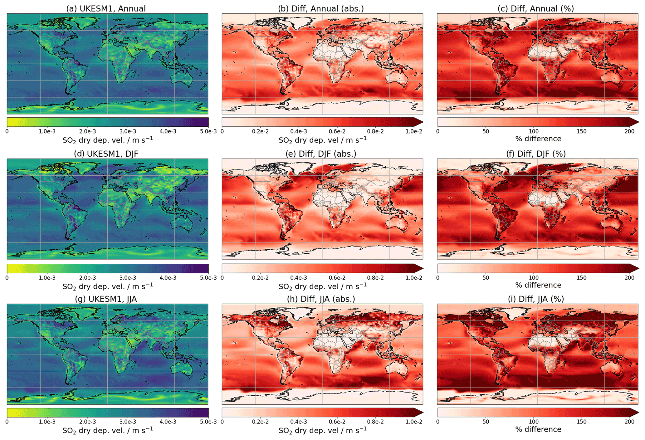
Figure 10SO2 dry deposition velocity for UKESM1 (a, d, g), absolute difference in SO2 dry deposition velocity for UKESM1-SO2 – UKESM1 (b, e, h), and percentage difference in SO2 dry deposition velocity for UKESM1-SO2 – UKESM1 (c, f, i). Annual means are shown in (a)–(c), the DJF mean is shown in (d)–(f), and the JJA mean is shown in (g)–(i). Each plot shows mean data for the period 1987–2014. Deposition velocity is calculated from the simulated surface SO2 and dry deposition flux values and represents the “bulk” deposition velocity for each model grid cell.
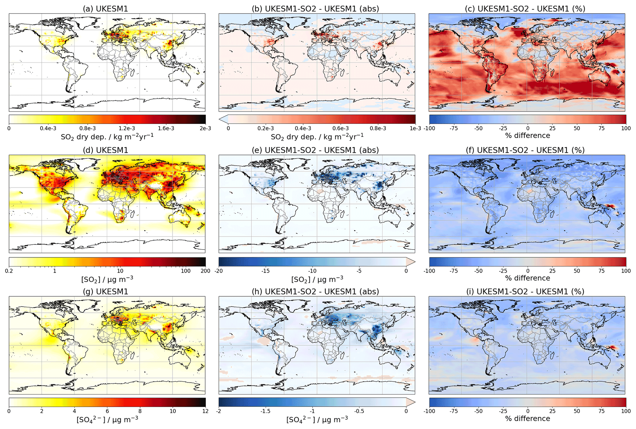
Figure 11SO2 dry deposition (a–c), surface SO2 concentration (d–f), and surface concentration (g–i) for UKESM1 (a, d, g), absolute difference for UKESM1-SO2 – UKESM1 (b, e, h), and percentage difference for UKESM1-SO2 – UKESM1 (c, f, i). In the plots showing absolute difference, areas where SO2 dry deposition is reduced in UKESM1-SO2 compared with UKESM1 are shown in blue (b), and areas where surface SO2 and concentrations are greater in UKESM1-SO2 compared with UKESM1 are shown in red (e, h). The blue shading in (b) and the red shading in (e) and (h) is not to scale as the absolute differences are very small. Each plot shows mean data for the period 1987–2014.
The increased SO2 dry deposition velocities in UKESM1-SO2 drive an increase in the SO2 dry deposition flux of nearly 45 % (from 29.49 to 42.56 T g yr−1) and subsequently reduce the SO2 lifetime by approximately 25 % (see Table C1). Overall the global SO2 burden is reduced from 0.54 to 0.41 T g yr−1. The full budget breakdown for SO2 is given in Appendix C (Table C1). The spatial distribution of these changes is illustrated in Fig. 11, which shows that SO2 dry deposition increases over most regions, with a corresponding decrease in surface SO2 concentrations. The lower SO2 burden then drives lower oxidation fluxes (Table C1), reducing the surface concentrations (Fig. 11g–i).
The largest absolute increases in SO2 dry deposition occur over the main source regions of USA–E, eastern China, and central and eastern Europe (Fig. 11b). However, Fig. 11c shows that the largest relative changes in dry deposition are over the ocean. Although the absolute changes over the ocean are small ( kg m−2 yr−1), the large global surface area of the ocean means that this increase is important for the global sulfur cycle. In UKESM1-SO2 Rsurf-mod increases the length of time land surfaces remain wet after rainfall, thus increasing SO2 dry deposition over most land surfaces (as seen in Fig. 11b) due to the high solubility of SO2 in water. Note that Rsurf-mod also makes SO2 dry deposition a function of the soil moisture content, and this aspect of the change drives decreases in SO2 dry deposition of 20 %–40 % over desert regions, such as the Sahara and high northern latitudes (see Fig. 11b and c). Conversely Rsurf-mod does not impact ocean surfaces, and the increases in SO2 dry deposition over oceans are driven by Rwater-mod.
The largest absolute reductions in mean annual surface SO2 and concentrations are over the source regions, corresponding to the locations of the largest increases in SO2 dry deposition. This is expected because dry deposition of SO2 to the surface is directly proportional to the surface concentration (Eq. 1). Figure 11e shows that mean annual surface SO2 concentration was reduced by up to 20 µg m−3 in the eastern USA, eastern China, and central and eastern Europe, which corresponds to a percentage decrease of 30 %–50 %. Note that this is similar to the percentage decrease in mean annual surface SO2 concentration over remote and ocean regions, although the absolute fluxes are much larger over the source regions. With the exception of some areas in the Sahara and the Middle East, we do not see increases in mean annual surface SO2 concentration where dry deposition fluxes decrease (albeit by very low amounts), such as the Arctic. We suggest that this is because these areas are remote and contain no SO2 sources, and by reducing SO2 in the source regions, we reduce overall atmospheric SO2 loading, and therefore less is transported to remote areas. Figure 11h and i show that mean annual surface concentrations are also reduced over the main source regions, although the reductions over the USA are relatively small compared with the other large source regions (0.5 µg m−3 compared with up to 3 µg m−3 in central and eastern Europe and China). Proportionally, the reduction in mean annual surface concentration is smaller than that for mean annual SO2 concentration, with decreases generally less than 5 % over most source regions.
4.2 Evaluation of UKESM1-SO2 against ground-based observations
In Fig. 12 and Table 7 we evaluate UKESM1-SO2 against the ground-based observations of mean annual surface SO2 and concentrations for the USA and European regions over the period from 1987 to 2014. UKESM1-SO2 is also evaluated against SO2 dry deposition flux from CASTNet over the same period. Figure 12a and b show that SO2 dry deposition flux is increased in UKESM1-SO2 relative to UKESM1, with this increase being more pronounced over USA–E compared with USA–W (see also Table 7). The increase in SO2 dry deposition in UKESM1-SO2 does enhance the model's over-prediction of this parameter relative to the CASTNet data, with NMB increasing from 1.15 in UKESM1 to 3.0 in UKESM1-SO2. Mean annual SO2 dry deposition fluxes are very low over USA–W due to the much lower concentrations of SO2 in this region. UKESM1 does over-predict mean annual SO2 dry deposition flux in this region too, but the absolute bias changes very little in UKESM1-SO2 (see Table 7). Figure 12c–e show that model bias in mean annual surface SO2 concentration is reduced in UKESM1-SO2 compared with UKESM1 in all three regions over the period 1987–2014. The largest absolute reduction is in USA–E, where mean annual surface SO2 concentration decreases from 20.05 to 14.10 µg m−3; however, the largest reduction in NMB is in USA–W, where it decreases from 12.54 to 9.52 (see Table 7). The model's over-prediction of mean annual surface concentration is reduced over USA–W in UKESM1-SO2 compared with UKESM1, with NMB decreasing from 0.72 to 0.41. However, the model's under-prediction of mean annual surface concentration over USA–E and Europe increases, with NMB = −0.31 in UKESM1 and NMB = −0.47 in UKESM1-SO2 (see Table 7). We find that the changes to the surface concentration and dry deposition flux occur almost uniformly over the seasonal cycle and so do not change the patterns in seasonal bias that are described in Sect. 3.4 for surface SO2 and concentrations.
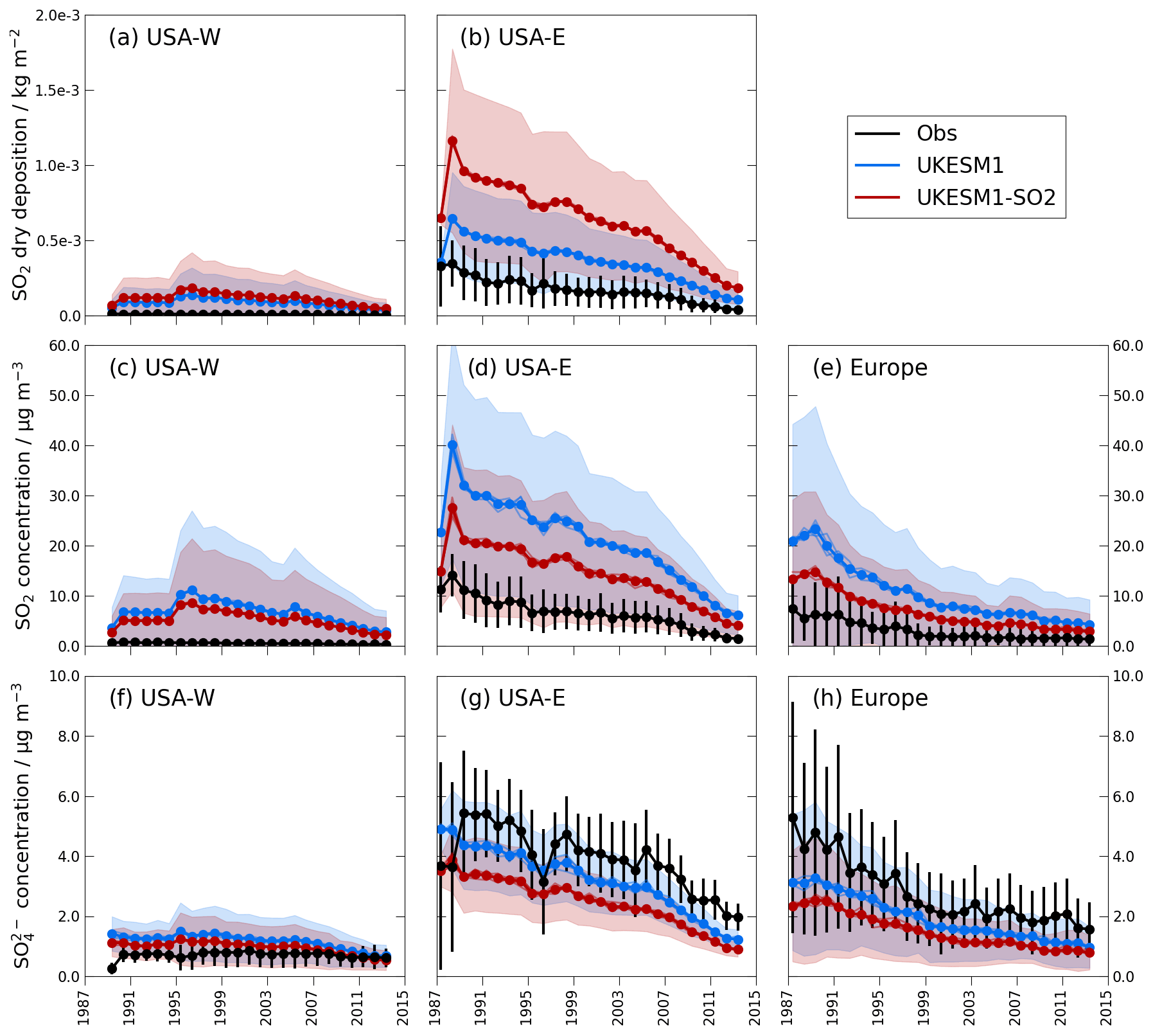
Figure 12Time series of observed and modelled mean annual SO2 dry deposition flux (a, b), surface SO2 concentration (c–e), and concentration (f–h) for USA–W (a, c, f; N sites = 16), USA–E (b, d, g; N sites = 33), and Europe (e, h; N SO2 sites = 48 and N sites = 42). No SO2 dry deposition flux observations are available for Europe.
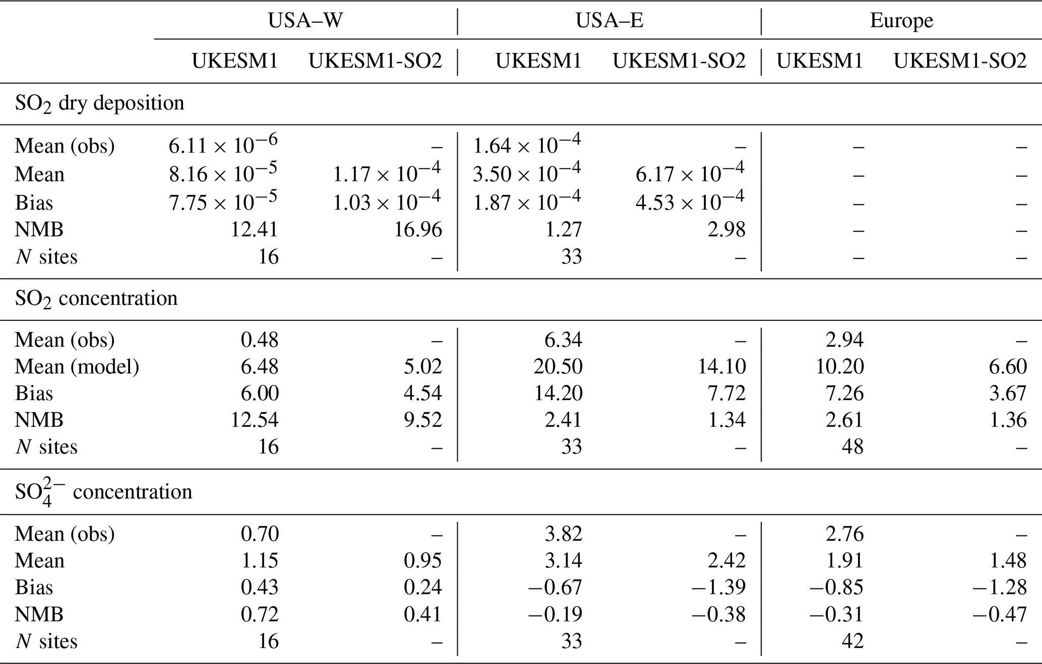
Table 7Statistics for mean annual surface SO2 and concentrations and SO2 dry deposition flux for UKESM1 and UKESM1-SO2. The mean seasonal values are averaged over the period 1987–2014. The units for SO2 and concentrations are µg m−3 and the units for SO2 dry deposition flux are kg m−2 yr−1 for SO2.
4.3 Evaluation of UKESM1-SO2 against TCSO2 observations
The impacts of the modifications to the SO2 dry deposition parameterization on TCSO2 are shown in Fig. 13 and Table 6. Figure 13a and b show that TCSO2 over the source regions is lower in UKESM1-SO2 relative to UKESM1 by 0.1–0.5 DU in DJF and JJA. This results in UKESM1-SO2 having a smaller positive bias in TCSO2 of +0.3 to +0.5 DU compared with that of +0.6 to +1.0 DU for UKESM1 (Fig. 13c and d; Sect. 3.5 and Fig. 8). This represents a decrease in the global TCSO2 model–OMI bias of 20 %–30 %. Over the outflow regions (e.g. off the US eastern seaboard), TCSO2 has reduced by 30 %–50 % and, over the source regions, this varies by 30 %–50 % for South to North-east Asia, 20 %–30 % for Europe, and 10 %–30 % for the USA (see Table 6). However, Fig. 13c and d also show that the inter-model differences are smaller than the existing model–satellite difference; i.e. the hatched regions are sporadic with limited coverage.
The evaluation of UKESM1 against ground-based observations of SO2 and concentrations from the USA and Europe, as well as SO2 dry deposition fluxes from the USA, shows that the model is able to represent recent historical changes in these variables. UKESM1 is also able to capture the spatial patterns in surface SO2 and concentrations and SO2 dry deposition, simulating larger values close to the sources and lower values away from the sources. However, UKESM1 generally over-predicts surface SO2 concentrations and dry deposition fluxes while under-predicting surface concentrations for the period 1987–2014. Further, we find that UKESM1 over-predicts the rate at which the surface SO2 concentrations decrease over this period.
We also make use of the updated TCSO2 product from OMI to evaluate UKESM1, finding that the model captures spatial patterns in TCSO2 at the global scale. Importantly, this evaluation allows us to identify model bias in regions without long-term ground-based networks, showing that UKESM1 over-predicts TCSO2 over all source and outflow regions. We find that although the ground-based and satellite observations are subject to different uncertainties, UKESM1's relative over-prediction of both surface SO2 concentration and TCSO2 is similar in the USA and Europe. This suggests that our finding of positive bias in modelled atmospheric SO2 is robust. We have also demonstrated that a more realistic treatment of SO2 dry deposition in UKESM1 reduces the model's atmospheric loading of SO2 and . However, we find that UKESM1's under-prediction of surface concentrations and over-prediction of SO2 dry deposition fluxes increases when the changes are included in the model, suggesting that there are further uncertainties in UKESM1's representation of the complex sulfur cycle processes. Additionally, the spatial and temporal differences in the model bias suggest that the drivers of model bias are regionally and seasonally dependent.
Broadly, a model's over-prediction of atmospheric SO2 can be driven by too little removal of SO2 (via deposition or oxidation) or overly high emissions. UKESM1 uses SO2 emissions from CMIP6 (Eyring et al., 2016). In comparing these emissions with the HTAP-OMI (Liu et al., 2018) and EDGAR (Crippa et al., 2018) data sets, Pope and Chipperfield (2021) showed that the total SO2 emissions in CMIP6 (115 Tg yr−1) are moderately larger than the HTAP-OMI (100 Tg yr−1) and EDGAR data sets (102 Tg yr−1). In general the CMIP6 emissions are larger than the HTAP-OMI and EDGAR emissions over all major source regions by up to kg m−2 yr−1. Exceptions occur at a number of point locations, which are likely from OMI rather than HTAP (Liu et al., 2018). Additionally, Smith (2021) has reported that SO2 emissions over the western USA are too high, possibly because the proxy data used to spatially distribute emissions do not take into account lower sulfur coal used in power plants and industry in this region.
Emission injection height is also an important constraint on near-surface SO2 concentrations, as demonstrated by Yang et al. (2019). This study found that uncertainty in industrial emission height resulted in modelled near‐surface SO2 concentrations varying between 70 % and 130 % over most land regions, higher than the overall uncertainty of 8 %–14 % attributed to SO2 emission rates. The SO2 injection height in UKESM1 was investigated by Mulcahy et al. (2020), who used injection heights prescribed as for HadGEM-GC3.1, where 50 % of energy and industry sector emissions are injected into the atmosphere at a height of 500 m. Mulcahy et al. (2020) showed that the introduction of a vertical profile for SO2 emissions in UKESM1 had negligible impact on surface concentrations at measurement sites in Europe and the USA, suggesting an important role for the aerosol chemistry in these regions. Emitting the SO2 at higher altitudes will act to reduce surface SO2 concentrations and therefore a model's bias against surface observations of both SO2 concentration and SO2 dry deposition flux. However, Pope and Chipperfield (2021) showed that UKESM1's bias in TCSO2 increased when emission injection heights were increased. This also suggests that the CMIP6 emissions are too high and that using a vertical profile for the emissions to some extent shifts the model's bias in SO2 to higher altitudes. However, we note that using varying emission heights for SO2 did not affect column densities in the GEOS-5/GOCART model (Buchard et al., 2014). We suggest undertaking model experiments with different emission inventories and injection height profiles to cast light on the role of SO2 emissions in model bias in the sulfur cycle.
The two main removal pathways for SO2 are oxidation to sulfate and dry deposition to the Earth's surface. In this study we have evaluated a more realistic treatment of SO2 dry deposition in UKESM1 that accounts for the high solubility of SO2 in water. We find that this reduces the dry deposition lifetime and consequently reduces the overall SO2 burden and lifetime. This reduces positive model bias in surface SO2 concentrations in the USA and Europe and in TCSO2 across most of the globe. The changes have the largest impact over source regions because dry deposition flux is directly proportional to the atmospheric concentration of SO2. There is also a reduction in the SO2 oxidation lifetime which likely drives the reduced atmospheric loading of . However, the true impact of the changes to the dry deposition parameterization are confounded by model uncertainty in other aspects of the complex sulfur cycle as well as the inherent difficulties associated with evaluating a global model against point observations.
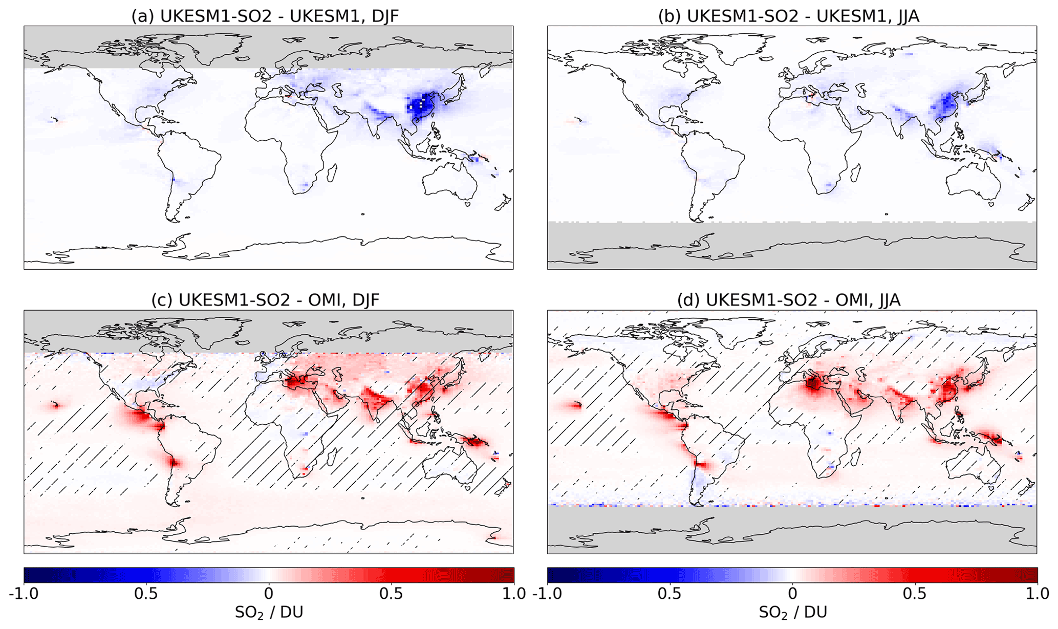
Figure 13Difference in TCSO2 between UKESM1 and UKESM-SO2 for DJF (a) and JJA (b). Difference in TCSO2 between UKESM1-SO2 and OMI for DJF (c) and JJA (d). Model and satellite data are averaged over the period 2005–2014. The hatched regions show where the inter-model differences are smaller than the existing model–satellite difference.
Dry deposition is a highly parameterized process and often poorly represented, particularly in global models. Similarly to UKESM1, Vet et al. (2014) showed that SO2 dry deposition fluxes were over-predicted by the 23-member model ensemble used for the TF-HTAP exercise relative to inferential data sets from measurement networks (including CASTNet). A key uncertainty highlighted in this study was that associated with the inferred dry deposition fluxes; from CASTNet these could be up to 30 % lower than direct observations of SO2 dry deposition flux (Baumgardner et al., 2002). However, the fluxes simulated by UKESM1 are a factor of 2 to 10 higher than the inferred data from USA–E and USA–W, indicating that the modelled deposition fluxes are almost certainly too large. Additional sources of uncertainty in model simulations of SO2 dry deposition may include land surface cover, changes in the atmospheric SO2 : NH3 ratio, and the ratio between wet and dry deposition of SO2. Mulcahy et al. (2020) showed that wet deposition, and to a lesser extent dry deposition, of SO2 was considerably lower in UKESM1 compared with HadGEM-GC3.1. Paulot et al. (2017) also report that poor representation of wet deposition likely contributed to bias in modelled surface concentrations. Overly low wet deposition would also contribute to the model's over-prediction of surface SO2 concentration. Dry deposition is sensitive to land surface type, which may not be well captured in global models. In this study the UKESM1 configuration uses 13 land cover classes, including 11 plant functional types (Archibald et al., 2020). This is reasonable for a global model, but inevitably detail is lost. Vet et al. (2014) also suggest that SO2 dry deposition may depend on the atmospheric NH3 loading. Long-term measurements at a UK site showed that SO2 dry deposition velocity has increased with time, which was attributed to changing ratios of SO2 : NH3 as SO2 concentrations have decreased more quickly than NH3 concentrations (Vet et al., 2014; Fowler et al., 2009). Currently nitrate chemistry is not represented in UKESM1, although it is planned for future model versions, and NH3 has not been evaluated in the model, so it is unknown how these factors may contribute to the model's bias in SO2 dry deposition flux and SO2 concentrations.
The role of uncertainty in sulfur cycle chemistry becomes apparent when we consider UKESM1's bias in surface concentrations in combination with the biases in SO2 concentrations and dry deposition. In Europe and USA–E, UKESM1 under-predicts surface concentrations, despite the large positive biases in SO2 concentrations through much of the period from 1987 to 2014. Note that there are exceptions close to certain point sources, particularly in Europe. However, in the cleaner USA–W region, surface concentrations are consistently over-predicted. We suggest that in USA–W overly high SO2 emissions (Smith, 2021), possibly in combination with overly low emission heights and the associated biases in dry deposition, drive the model's over-prediction of surface concentrations in this region. However, in the polluted regions of Europe and USA–E, the under-prediction of surface concentrations, despite large over-predictions of surface SO2 concentrations, suggests that sulfur cycle chemistry is not correctly represented, and Mulcahy et al. (2020) showed that there are global and regional differences in oxidant concentrations and in the SO2 lifetime between UKESM1 and the HadGEM-GC3.1 model, with the latter better able to capture surface concentrations. In reducing the SO2 burden, we further reduce its overall lifetime and oxidation lifetime relative to HadGEM-GC3.1. This highlights the requirement for a more detailed investigation of SO2 oxidation in UKESM1, particularly in polluted regions.
Uncertainty in UKESM1's sulfur chemistry also appears to be seasonally dependent. In USA–E and Europe UKESM1 over-predicts SO2 (surface concentration and TCSO2) and under-predicts surface at all times of the year, but there is seasonal variation in these biases. In Europe, the model bias is largest in DJF, which drives a stronger seasonal cycle relative to the observations. This is in agreement with Turnock et al. (2015), who investigated in an earlier HadGEM3-UKCA configuration. The seasonality in UKESM1's bias over Europe may be due to the model under-predicting in-cloud SO2 oxidation via O3 (Table 1). In winter and at higher latitudes this reaction is likely to be the dominant removal pathway due to lower availability of H2O2 (Turnock et al., 2019). However, the picture is different in USA–E, where UKESM1 over-predicts SO2 to a larger extent in JJA compared with DJF, and there is little seasonality in the model's under-prediction . In USA–E it is likely that uncertainty in UKESM1's representation of SO2 oxidation via both O3 and H2O2 (Table 1) contributes to bias in SO2 and . The lower average latitude of the USA–E sites compared with the European sites means that the O3 oxidation pathway is more important in this region, and it has been demonstrated that concentrations are sensitive to both pathways in winter (Paulot et al., 2017). From this study it is not clear what is driving the relatively large positive bias in SO2 in JJA over USA–E, and we stress the need for closer examination of the sulfur chemistry in UKESM1.
Recent studies have also shown that cloud water pH may be an important factor in the aqueous-phase oxidation of SO2 to (Turnock et al., 2019). While a temporally and spatially uniform cloud pH of 5 is currently used in UKESM1, observations of this quantity show that it varies in space and time. Observations at an American site showed that mean cloud pH increased from 4 to 4.8 between 1994 and 2014 (Schwab et al., 2016), cloud pH measured at Mt Tai in North China from 2007 to 2008 was between 3.56 and 7.64, and measurement campaigns between 1985 and 2008 at various European, North American, and East Asian locations reported values between 3.34 and 5.29 (Guo et al., 2012). Turnock et al. (2019) showed that varying this value in the HadGEM3-UKCA model can have a large impact on SO2 and concentrations. Over source regions, including Europe and North America, increasing the cloud water pH by 1.0 reduced the annual mean global SO2 column burden by approximately 50 %, as more SO2 was oxidized in cloud droplets, and consequently there were small increases in the annual mean sulfate column burden over these regions. Conversely, outside of polluted regions, increasing the cloud water pH reduced the sulfate column burden by 10 % to 40 % globally. These results indicate that having a more realistic treatment of cloud water pH could reduce UKESM1's biases in TCSO2 and potentially in SO2 and concentrations remote from source regions. However, it is unlikely to be a dominant removal pathway at the surface, and any impact on surface SO2 concentrations, especially close to sources, would likely be minimal.
In an Earth system model such as UKESM1, there are inevitably some compromises in the complexity of the chemistry and aerosol schemes, as these are computationally expensive. While the sulfur chemistry represented in the UKCA-StratTrop model used in UKESM1 accounts for important SO2 and DMS oxidation reactions as well as simulating oxidants (rather than the offline oxidant scheme used in HadGEM-GC3.1), it cannot be complete. In the recently developed CRI-Strat scheme the sulfur chemistry reactions are as for UKCA-StratTrop, but there is a more comprehensive treatment of non-methane volatile compounds (NMVOCs) (Archer-Nicholls et al., 2020), resulting in higher surface ozone concentrations, particularly over polluted areas in summer, compared with UKCA-StratTrop. As demonstrated by Mulcahy et al. (2020), the increased oxidants in UKESM1 relative to HadGEM-GC3.1 likely contribute to reducing the SO2 lifetime from 4.29 to 3.86 d. CRI-Strat is compatible with UKESM1, and the higher oxidant loading may reduce SO2 oxidation lifetime further with a concurrent increase in . Model bias in remote ocean regions may also result from the necessarily simplified DMS oxidation chemistry in UKESM1. A more detailed representation of DMS chemistry over the Southern Ocean was investigated by Revell et al. (2019), who found that surface SO2 concentrations increased over the Southern Ocean, possibly due to including reactions between DMS and halogen species, while concentrations decreased, likely as a result of there being more DMS oxidation reactions.
Model resolution is also likely to be an important source of model bias in this study. In evaluating UKESM1 against the CASTNet and EMEP data sets we are comparing a simulated value generated from a model grid box at a scale of ≈ 200–300 km with a point observation. This may be a particular problem for the surface SO2 concentrations and SO2 dry deposition fluxes because in reality a large fraction (20 %–40 %) of SO2 emitted from point sources is lost in the first 100 km, which is sub-grid scale relative to the model grid boxes (Smith and Jeffrey, 1975; Wys et al., 1978). In UKESM1 the sub-grid scale loss is not captured because SO2 is evenly emitted across the grid box and deposition is subsequently calculated. Potentially this drives overall large model biases compared with ground-based observations that are not necessarily close to the point sources. In addition, the model resolution can not capture complex orography, meaning that transport of SO2 may not be well represented. This could be problematic in mountainous areas of USA–W (VanCuren and Gustin, 2015). High-resolution model studies would be beneficial to address the both importance of orography and to investigate the SO2 losses close to sources. We also suggest that evaluating UKESM1 against chemical re-analysis fields of SO2 could reduce some of the bias that occurs with using point observations, but there are uncertainties associated with this approach too (Ukhov et al., 2020).
We evaluate UKESM1 against ground-based and satellite observations of selected sulfur species over the recent historical period. We find that UKESM1 is able to capture the temporal and spatial patterns in surface SO2, surface sulfate concentration, SO2 dry deposition, and TCSO2. However, compared with observations, we find that the model is biased, depending on the variable, region, and species. We address one possible source of bias by introducing a more realistic treatment of SO2 dry deposition, a key loss process for this species. This change reduces model bias in surface SO2 concentrations and TCSO2. However, it is apparent that other biases exist within the complex sulfur cycle, and we highlight some key areas for further investigation and development.
Our evaluation suggests that uncertainty in UKESM1's sulfur chemistry is also an important driver of the biases seen in this study, particularly over polluted regions. Two priorities for further investigation into the oxidation of SO2 in UKESM1 are (i) an evaluation of the CRI-Strat scheme and (ii) a more realistic treatment of cloud water pH. The model's necessarily limited DMS chemistry may also contribute to bias in atmospheric sulfur loading over remote ocean areas. The impact of the nitrate scheme currently in development for UKESM1 will also be investigated in relation to the sulfur cycle. Another aspect of UKESM1's sulfur cycle that would benefit from more detailed analysis is the ratio between wet and dry deposition and how this compares with observations. We also suggest that high-resolution studies to investigate SO2 deposition close to sources would be beneficial for a better understanding of these processes. Finally, we suggest that the SO2 emissions may be too high through a possible combination of overly high emissions in the CMIP6 inventory and injection of the emissions into the surface layer only.
The sulfur cycle is a key area of analysis and development for UKESM1 given its importance as a driver of historical aerosol forcing. UKESM1 is relatively unique amongst models in CMIP6 in that it has a fully interactive atmospheric chemistry scheme coupled to a two-moment (mass and number) aerosol scheme. Given the complexity of the model's chemistry-aerosol treatment within the ES framework, the model's performance here is encouraging and provides confidence in UKESM1, particularly in regard to capturing the historical trend. However, there is always space for improvement, and to the more realistic treatment of SO2 dry deposition will therefore be incorporated into the planned release of UKESM1.1. This latest model version will be documented in a forthcoming publication which will also address the impact of the SO2 dry deposition changes on aerosol loading and climate.
Here we describe in detail the changes to UKESM1's parameterization of dry deposition of SO2 to the surface. These modifications account for the impact of surface wetness due to rainfall or humidity on SO2 dry deposition to vegetated or soil surfaces. We first derive a parameter, zwet, which designates whether a model grid box at time step N is wet or dry. We assume that on entering time step N the grid box in question has a dry surface (zwet = 0). If, during time step N, precipitation is greater than a threshold value (set to 0.5 mm d−1), the grid box then becomes classed as wet (zwet = 1). Once precipitation stops, the grid box is assumed to dry out over a specified period. Assuming no precipitation falls during this drying period, at the end of the period the grid box will be classed as dry (zwet = 0). If, during the drying period, a new precipitation event occurs at the grid box of intensity greater than 0.5 mm d−1, zwet is reset to 1. If the precipitation event is less than 0.5 mm d−1 but greater than 0.0 mm d−1, zwet is not reset to 1, and neither is it decreased in value (i.e. no drying is assumed to occur over that time step). A grid box is classed as wet whenever zwet > 0. We tested a range of time periods from 3 h to 1 d and found only minor sensitivity to this parameter. For UKESM1-SO2 we used a drying period of 3 h. In future work we will investigate making this parameter a function of surface evaporation and downwelling solar radiation.
If a grid box is classed as wet, then Rsoil and Rcut (for all vegetation types) are set equal to 1 s m−1. Through Eq. (5), Rc will then tend towards a value of 1 s m−1, equating to minimal resistance to SO2 deposition. In these situations, the amount of SO2 deposited will primarily be limited by the efficiency of gas transport to the receptor surface, i.e. by Ra and Rb in Eq. (2). If the grid box is classed as dry, Rcut is calculated following Eq. (9) in Erisman et al. (1994), whereby Rcut is a decreasing function of near-surface relative humidity. If a grid box surface temperature lies between −1 and −5 ∘C, Rcut is reset to 200 s m−1 and below −5 ∘C to 500 s m−1, irrespective of the near-surface relative humidity. For dry grid boxes, Rsoil uses a value of 213.5 s m−1 for all surface temperatures (see Table A2). For dry surfaces, Rcut also approaches a value of 1 s m−1 as near-surface relative humidity approaches a value of 1. As for a wet surface, under these conditions there is minimal resistance to SO2 deposition, and Rc will tend towards 1 s m−1. Thus SO2 dry deposition will primarily be limited by Ra and Rb.
Table A1Summary of the representation of Rcut and Rsoil in UKESM1 and UKESM1-SO2. Units for resistance values are s m−1.
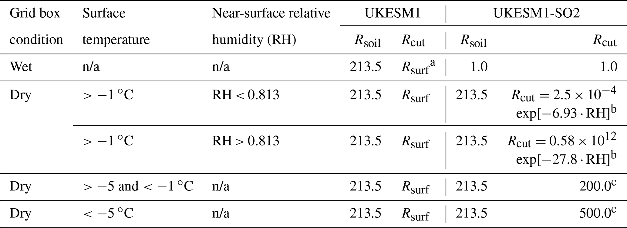
a See values in Table A2. b Following Erisman et al. (1994). c Irrespective of near-surface relative humidity. n/a – not applicable.
Table A2Standard surface resistance (Rsurf) values for SO2 for land use types in UKESM1. These values were calculated based on the data published in Zhang et al. (2003) for SO2.
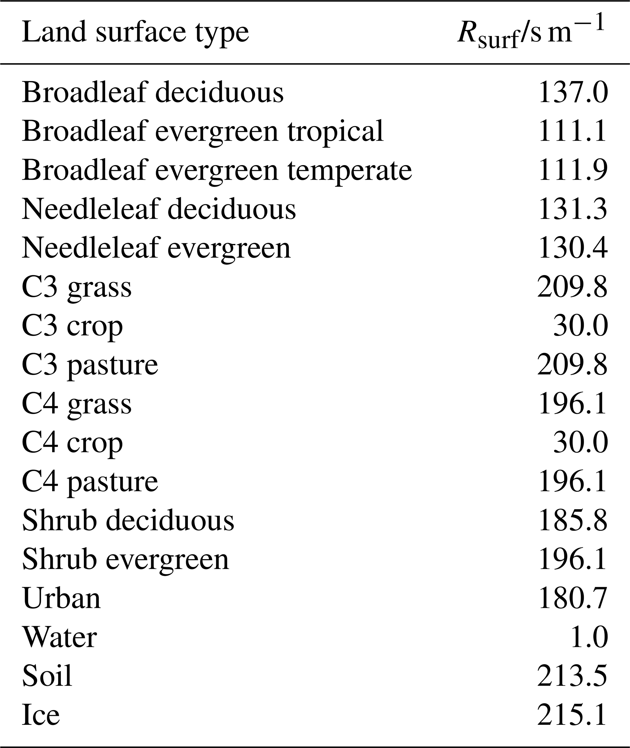
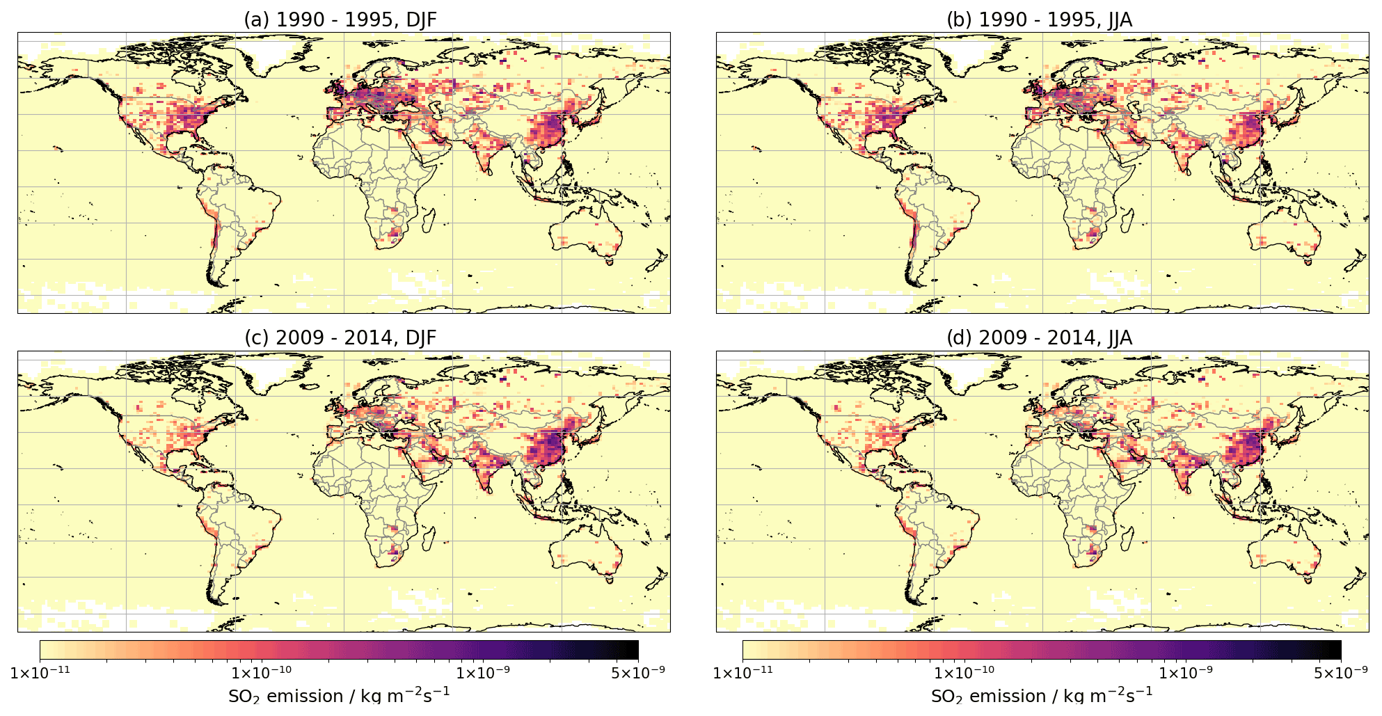
Figure B1Global emissions of SO2 used in UKESM1. Mean seasonal emissions are shown for the 1990–1995 time slice for DJF (a) and JJA (b) and the 2009–2014 time slice for DJF (c) and JJA (d).
Table C1Global SO2 budget for UKESM1 and UKESM1-SO2. Units for production and loss fluxes are in Tg [S] yr−1, burdens are in Tg, and lifetimes are in days. The values are calculated from a 2-year AMIP simulation covering the period 1981–1983 inclusive.
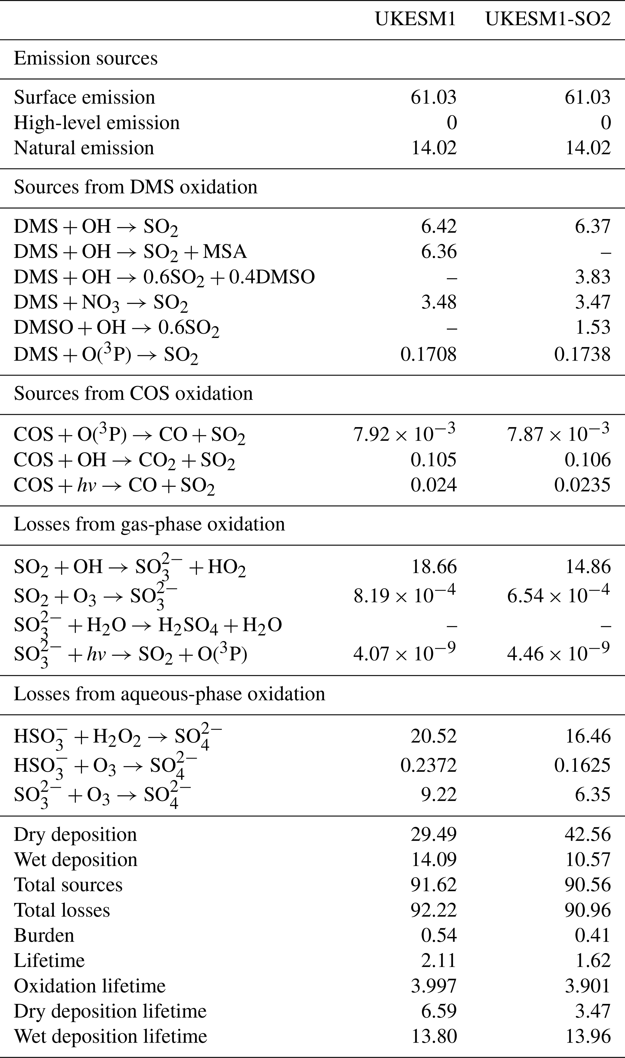
The UM is the source code for the atmosphere–land–ocean–sea ice components of the UKESM1 physical model, including the NEMO and CICE modules for oceans and sea ice respectively. The UM source code base also houses the GLOMAP-Mode and UKCA modules. JULES is the source code for land and terrestrial biogeochemistry components. MEDUSA is the source code for the ocean biogeochemistry. Due to intellectual property rights restrictions, we cannot provide either the source code or documentation papers for the UM or JULES. Obtaining the UM. The Met Office Unified Model is available for use under licence. A number of research organizations and national meteorological services use the UM in collaboration with the Met Office to undertake basic atmospheric process research, produce forecasts, develop the UM code, and build and evaluate Earth system models. For further information on how to apply for a licence, see http://www.metoffice.gov.uk/research/modelling-systems/unified-model (last access: 17 March 2021). Obtaining JULES. JULES is available under licence, free of charge. For further information on how to gain permission to use JULES for research purposes, see https://jules-lsm.github.io/access_req/JULES_access.html (last access: 14 December 2021). Information about the UKESM1 release and its components and the prerequisites for using it can be found here: http://cms.ncas.ac.uk/wiki/UM/Configurations/UKESM (last access: 14 December 2021). Briefly, UKESM1 is distributed and run as a Rose suite on the Archer2 and Monsoon computing platforms administered by UK Research Innovation (UKRI) and the Met Office/Natural Environment Research Council (NERC) respectively. Rose is a framework for developing and running meteorological applications and is described in more detail here: http://cms.ncas.ac.uk/wiki/RoseCylc, last access: 14 December 2021, (NCAS Computational Modelling Services, 2018).
The simulation data used in this study are archived on the Earth System Grid Federation (ESGF) node (https://esgf-node.llnl.gov/projects/cmip6/, last access: 14 December 2021, Earth System CoG sponsors and partners, 2019). The model source ID is UKESM1-0-LL for UKESM1. UKESM1 historical simulations are identified by the following variant labels: r1i1p1f2, r2i1p1f2, r8i1p1f2, and r9i1p1f2 (https://doi.org/10.22033/ESGF/CMIP6.6113; Tang et al., 2019). We acknowledge the use of the CASTNet database (https://www.epa.gov/castnet, last access: 14 December 2021, United States Environmental Protection Agency, 2021). Information on the EMEP network can be found in Tørseth et al. (2012, https://doi.org/10.5194/acp-12-5447-2012), and the data are available from http://ebas.nilu.no/. OMI total column SO2 data were obtained from NASA's Goddard Earth Sciences Data and Information Services Center (GES DISC, https://disc.gsfc.nasa.gov/, last access: 14 December 2021, NASA Goddard Earth Sciences (GES) Data and Information Services Center, 2021).
CGJ, JPM, STT, and CH contributed to the conceptualization of this study. CGJ and STR developed and tested the code changes for the revised dry deposition parameterization. STR ran the UKESM1 and UKESM1-SO2 historical simulations. CJ ran the UKESM1 and UKESM1-SO2 AMIP simulations and calculated the SO2 budgets. CH led the analysis and did the data visualization. RJP with support from CL evaluated UKESM1 against the OMI SO2 product. CH led the preparation of the manuscript, with important text contributions from JPM, CGJ, and RJP. All the co-authors contributed invaluable comments in reviewing and editing the manuscript.
The contact author has declared that neither they nor their co-authors have any competing interests.
Publisher’s note: Copernicus Publications remains neutral with regard to jurisdictional claims in published maps and institutional affiliations.
For making their measurement data available to be used in this study, we would like to thank the EMEP and CASTNet measurement networks along with any data managers involved in data collection. The EBAS database has largely been funded by the UN-ECE CLRTAP (EMEP), AMAP, and NILU internal resources. Specific developments have been possible due to projects like EUSAAR (EU-FP5) (EBAS web interface), EBAS-Online (Norwegian Research Council INFRA) (upgrading of the database platform), and HTAP (European Commission DG-ENV) (import and export routines to build a secondary repository in support of http://www.htap.org, last access: 14 December 2021). The US Environmental Protection Agency is the primary funding source for CASTNet, with contracting and research support from the National Park Service. This study used JASMIN, the UK's collaborative data analysis environment (http://jasmin.ac.uk, last access: 14 December 2021) (Lawrence et al., 2013). Catherine Hardacre made extensive use of the Iris and Cartopy libraries for the analysis and data visualization in this study (Met Office, 2010–2013, 2010–2015).
This research has been supported by the UK government, BEIS and DEFRA (grant no. GA01101), the National Environment Research Council (NERC), and the National Capability Science Multi-Centre (NCSMC) (UKESM grant no. NE/N017978/1). Colin Johnson was funded by EU Horizon 2020 project CRESCENDO, grant no. 641816. Richard J. Pope was supported by the UK Natural Environment Research Council (NERC) by providing funding for the National Centre for Earth Observation (NCEO) through grant no. NE/R016518/1. Steven T. Turnock was supported by the UK–China Research and Innovation Partnership Fund through the Met Office Climate Science for Service Partnership (CSSP) China as part of the Newton Fund. OMI SO2 product development and analysis were supported by the NASA Earth Science Division (ESD) Aura Science Team program (grant no. 80NSSC17K0240).
This paper was edited by Leiming Zhang and reviewed by two anonymous referees.
Aas, W., Mortier, A., Bowersox, V., Cherian, R., Faluvegi, G., Fagerli, H., Hand, J., Klimont, Z., Galy-Lacaux, C., Lehmann, C. M. B., Myhre, C. L., Myhre, G., Olivie, D., Sato, K., Quaas, J., Rao, P. S. P., Schulz, M., Shindell, D., Skeie, R. B., Stein, A., Takemura, T., Tsyro, S., Vet, R., and Xu, X.: Global and regional trends of atmospheric sulfur, Sci. Rep.-UK, 9, 953, https://doi.org/10.1038/s41598-018-37304-0, 2019. a, b, c, d, e
Aleksic, N., Roy, K., Sistla, G., Dukett, J., Houck, N., and Casson, P.: Analysis of cloud and precipitation chemistry at Whiteface Mountain, NY, Atmos. Environ., 43, 2709–2716, 2009. a
Altshuller, A.: Model predictions of the rates of homogeneous oxidation of sulfur dioxide to sulfate in the troposphere, Atmos. Environ., 13, 1653–1661, https://doi.org/10.1016/0004-6981(79)90323-8, 1979. a
Archer-Nicholls, S., Abraham, N. L., Shin, Y. M., Weber, J., Russo, M. R., Lowe, D., Utembe, S., O'Connor, F. M., Kerridge, B., Latter, B., Siddans, R., Jenkin, M., Wild, O., and Archibald, A. T.: The Common Representative Intermediates Mechanism version 2 in the United Kingdom Chemistry and Aerosols Model, J. Adv. Model. Earth Syst., 13, e2020MS002420, https://doi.org/10.1029/2020MS002420, 2020. a
Archibald, A. T., O'Connor, F. M., Abraham, N. L., Archer-Nicholls, S., Chipperfield, M. P., Dalvi, M., Folberth, G. A., Dennison, F., Dhomse, S. S., Griffiths, P. T., Hardacre, C., Hewitt, A. J., Hill, R. S., Johnson, C. E., Keeble, J., Köhler, M. O., Morgenstern, O., Mulcahy, J. P., Ordóñez, C., Pope, R. J., Rumbold, S. T., Russo, M. R., Savage, N. H., Sellar, A., Stringer, M., Turnock, S. T., Wild, O., and Zeng, G.: Description and evaluation of the UKCA stratosphere–troposphere chemistry scheme (StratTrop vn 1.0) implemented in UKESM1, Geosci. Model Dev., 13, 1223–1266, https://doi.org/10.5194/gmd-13-1223-2020, 2020. a, b, c, d, e
Baldocchi, D. D., Hicks, B. B., and Camara, P.: A canopy stomatal resistance model for gaseous deposition to vegetated surfaces, Atmos. Environ., 21, 91–101, 1987. a
Baumgardner, R., Lavery, T., Rogers, C., and Isil, S.: Estimates of the atmospheric deposition of sulfur and nitrogen species: Clean Air Status and Trends Network, 1990–2000, Environ. Sci. Technol., 36, 2614–2629, https://doi.org/10.1021/es011146g, 2002. a, b, c, d, e, f, g
Best, M. J., Pryor, M., Clark, D. B., Rooney, G. G., Essery, R. L. H., Ménard, C. B., Edwards, J. M., Hendry, M. A., Porson, A., Gedney, N., Mercado, L. M., Sitch, S., Blyth, E., Boucher, O., Cox, P. M., Grimmond, C. S. B., and Harding, R. J.: The Joint UK Land Environment Simulator (JULES), model description – Part 1: Energy and water fluxes, Geosci. Model Dev., 4, 677–699, https://doi.org/10.5194/gmd-4-677-2011, 2011. a
Boucher, O., Randall, D., Artaxo, P., Bretherton, C., Feingold, G., Forster, P., Kerminen, V.-M., Kondo, Y., Liao, H., Lohmann, U., Rasch, P., Satheesh, S. K., Sherwood, S., Stevens, B., and Zhang, X. Y.: Clouds and aerosols, in: Climate change 2013: the physical science basis. Contribution of Working Group I to the Fifth Assessment Report of the Intergovernmental Panel on Climate Change, Cambridge University Press, 571–657, https://doi.org/10.1017/CBO9781107415324, 2013. a
Buchard, V., da Silva, A. M., Colarco, P., Krotkov, N., Dickerson, R. R., Stehr, J. W., Mount, G., Spinei, E., Arkinson, H. L., and He, H.: Evaluation of GEOS-5 sulfur dioxide simulations during the Frostburg, MD 2010 field campaign, Atmos. Chem. Phys., 14, 1929–1941, https://doi.org/10.5194/acp-14-1929-2014, 2014. a
Chin, M., Rood, R. B., Lin, S.-J., Müller, J.-F., and Thompson, A. M.: Atmospheric sulfur cycle simulated in the global model GOCART: Model description and global properties, J. Geophys. Res.-Atmos., 105, 24671–24687, https://doi.org/10.1029/2000JD900384, 2000. a, b
Clark, D. B., Mercado, L. M., Sitch, S., Jones, C. D., Gedney, N., Best, M. J., Pryor, M., Rooney, G. G., Essery, R. L. H., Blyth, E., Boucher, O., Harding, R. J., Huntingford, C., and Cox, P. M.: The Joint UK Land Environment Simulator (JULES), model description – Part 2: Carbon fluxes and vegetation dynamics, Geosci. Model Dev., 4, 701–722, https://doi.org/10.5194/gmd-4-701-2011, 2011. a
Clarke, J., Edgerton, E., and Martin, B.: Dry deposition calculations for the clean air status and trends network, Atmos. Environ., 31, 3667–3678, https://doi.org/10.1016/S1352-2310(97)00141-6, 1997. a, b, c, d, e
Crippa, M., Guizzardi, D., Muntean, M., Schaaf, E., Dentener, F., van Aardenne, J. A., Monni, S., Doering, U., Olivier, J. G. J., Pagliari, V., and Janssens-Maenhout, G.: Gridded emissions of air pollutants for the period 1970–2012 within EDGAR v4.3.2, Earth Syst. Sci. Data, 10, 1987–2013, https://doi.org/10.5194/essd-10-1987-2018, 2018. a, b, c
Dentener, F., Kinne, S., Bond, T., Boucher, O., Cofala, J., Generoso, S., Ginoux, P., Gong, S., Hoelzemann, J. J., Ito, A., Marelli, L., Penner, J. E., Putaud, J.-P., Textor, C., Schulz, M., van der Werf, G. R., and Wilson, J.: Emissions of primary aerosol and precursor gases in the years 2000 and 1750 prescribed data-sets for AeroCom, Atmos. Chem. Phys., 6, 4321–4344, https://doi.org/10.5194/acp-6-4321-2006, 2006. a
Dyer, A.: A review of flux-profile relationships, Bound.-Lay. Meteorol., 7, 363–372, 1974. a
Earth System CoG sponsors and partners: WCRP CMIP6 ESGF Node, ESGF [data set], available at: https://esgf-node.llnl.gov/projects/cmip6/ (last access: 14 December 2021), 2019. a
Erisman, J. W. and Baldocchi, D.: Modelling dry deposition of SO2, Tellus B, 46, 159–171, https://doi.org/10.1034/j.1600-0889.1994.t01-2-00001.x, 1994. a, b, c
Erisman, J. W., Pul, A. V., and Wyers, P.: Parametrization of surface resistance for the quantification of atmospheric deposition of acidifying pollutants and ozone, Atmos. Environ., 28, 2595–2607, https://doi.org/10.1016/1352-2310(94)90433-2, 1994. a, b, c
Eyring, V., Bony, S., Meehl, G. A., Senior, C. A., Stevens, B., Stouffer, R. J., and Taylor, K. E.: Overview of the Coupled Model Intercomparison Project Phase 6 (CMIP6) experimental design and organization, Geosci. Model Dev., 9, 1937–1958, https://doi.org/10.5194/gmd-9-1937-2016, 2016. a, b, c
Feng, L., Smith, S. J., Braun, C., Crippa, M., Gidden, M. J., Hoesly, R., Klimont, Z., van Marle, M., van den Berg, M., and van der Werf, G. R.: The generation of gridded emissions data for CMIP6, Geosci. Model Dev., 13, 461–482, https://doi.org/10.5194/gmd-13-461-2020, 2020. a, b, c
Finkelstein, P., Ellestad, T., Clarke, J., Meyers, T., Schwede, D., Hebert, E., and Neal, J.: Ozone and sulfur dioxide dry deposition to forests: Observations and model evaluation, J. Geophys. Res.-Atmos., 105, 15365–15377, https://doi.org/10.1029/2000JD900185, 2000. a, b
Fioletov, V. E., McLinden, C. A., Krotkov, N., Li, C., Joiner, J., Theys, N., Carn, S., and Moran, M. D.: A global catalogue of large SO2 sources and emissions derived from the Ozone Monitoring Instrument, Atmos. Chem. Phys., 16, 11497–11519, https://doi.org/10.5194/acp-16-11497-2016, 2016. a, b, c
Fowler, D.: Dry Deposition of SO2 on Agricultural Crops, in: Sulfur in the Atmosphere, edited by: Husar, R., Lodge, J., and Moore, D., 369–373, Pergamon, Oxford, UK, https://doi.org/10.1016/B978-0-08-022932-4.50041-0, 1978. a, b
Fowler, D., Pilegaard, K., Sutton, M. A., Ambus, P., Raivonen, M., Duyzer, J., Simpson, D., Fagerli, H., Fuzzi, S., Schjoerring, J. K., Granier, C., Neftel, A., Isaksen, I. S. A., Laj, P., Maione, M., Monks, P. S., Burkhardt, J., Daemmgen, U., Neirynck, J., Personne, E., Wichink-Kruit, R., Butterbach-Bahl, K., Flechard, C., Tuovinen, J. P., Coyle, M., Gerosa, G., Loubet, B., Altimir, N., Gruenhage, L., Ammann, C., Cieslik, S., Paoletti, E., Mikkelsen, T. N., Ro-Poulsen, H., Cellier, P., Cape, J. N., Horvath, L., Loreto, F., Niinemets, U., Palmer, P. I., Rinne, J., Misztal, P., Nemitz, E., Nilsson, D., Pryor, S., Gallagher, M. W., Vesala, T., Skiba, U., Brueggemann, N., Zechmeister-Boltenstern, S., Williams, J., O'Dowd, C., Facchini, M. C., de Leeuw, G., Flossman, A., Chaumerliac, N., and Erisman, J. W.: Atmospheric composition change: Ecosystems-Atmosphere interactions, Atmos. Environ., 43, 5193–5267, https://doi.org/10.1016/j.atmosenv.2009.07.068, 2009. a
Ganzeveld, L. and Lelieveld, J.: Dry deposition parameterization in a chemistry general circulation model and its influence on the distribution of reactive trace gases, J. Geophys. Res.-Atmos., 100, 20999–21012, 1995. a
Garland, J.: The dry deposition of sulphur dioxide to land and water surfaces, P. Roy. Soc. Lond. A Mat., 354, 245–268, 1977. a, b
Garland, J. A. and Branson, J. R.: The deposition of sulphur dioxide to pine forest assessed by a radioactive tracer method, Tellus, 29, 445–454, https://doi.org/10.1111/j.2153-3490.1977.tb00755.x, 1977. a, b
Guo, J., Wang, Y., Shen, X., Wang, Z., Lee, T., Wang, X., Li, P., Sun, M., Collett, J. L., Wang, W., and Wang, T.: Characterization of cloud water chemistry at Mount Tai, China: Seasonal variation, anthropogenic impact, and cloud processing, Atmos. Environ., 60, 467–476, https://doi.org/10.1016/j.atmosenv.2012.07.016, 2012. a
Hoesly, R. M., Smith, S. J., Feng, L., Klimont, Z., Janssens-Maenhout, G., Pitkanen, T., Seibert, J. J., Vu, L., Andres, R. J., Bolt, R. M., Bond, T. C., Dawidowski, L., Kholod, N., Kurokawa, J.-I., Li, M., Liu, L., Lu, Z., Moura, M. C. P., O'Rourke, P. R., and Zhang, Q.: Historical (1750–2014) anthropogenic emissions of reactive gases and aerosols from the Community Emissions Data System (CEDS), Geosci. Model Dev., 11, 369–408, https://doi.org/10.5194/gmd-11-369-2018, 2018. a, b, c
Holland, D. M., Principe, P. P., and Sickles, J. E.: Trends in atmospheric sulfur and nitrogen species in the eastern United States for 1989–1995, Atmos. Environ., 33, 37–49, https://doi.org/10.1016/S1352-2310(98)00123-X, 1998. a, b
Holtslag, A. A. M. and Bruin, H. A. R. D.: Applied Modeling of the Nighttime Surface Energy Balance over Land, J. Appl. Meteorol. Clim., 27, 689–704, https://doi.org/10.1175/1520-0450(1988)027<0689:AMOTNS>2.0.CO;2, 1988. a
Janssens-Maenhout, G., Crippa, M., Guizzardi, D., Dentener, F., Muntean, M., Pouliot, G., Keating, T., Zhang, Q., Kurokawa, J., Wankmüller, R., Denier van der Gon, H., Kuenen, J. J. P., Klimont, Z., Frost, G., Darras, S., Koffi, B., and Li, M.: HTAP_v2.2: a mosaic of regional and global emission grid maps for 2008 and 2010 to study hemispheric transport of air pollution, Atmos. Chem. Phys., 15, 11411–11432, https://doi.org/10.5194/acp-15-11411-2015, 2015. a, b, c
Karset, I. H. H., Berntsen, T. K., Storelvmo, T., Alterskjær, K., Grini, A., Olivié, D., Kirkevåg, A., Seland, Ø., Iversen, T., and Schulz, M.: Strong impacts on aerosol indirect effects from historical oxidant changes, Atmos. Chem. Phys., 18, 7669–7690, https://doi.org/10.5194/acp-18-7669-2018, 2018. a
Kipling, Z., Stier, P., Schwarz, J. P., Perring, A. E., Spackman, J. R., Mann, G. W., Johnson, C. E., and Telford, P. J.: Constraints on aerosol processes in climate models from vertically-resolved aircraft observations of black carbon, Atmos. Chem. Phys., 13, 5969–5986, https://doi.org/10.5194/acp-13-5969-2013, 2013. a
Kreidenweis, S. M., Walcek, C. J., Feingold, G., Gong, W., Jacobson, M. Z., Kim, C.-H., Liu, X., Penner, J. E., Nenes, A., and Seinfeld, J. H.: Modification of aerosol mass and size distribution due to aqueous-phase SO2 oxidation in clouds: Comparisons of several models, J. Geophys. Res.-Atmos., 108, D7, https://doi.org/10.1029/2002JD002697, 2003. a
Krotkov, N. A., McLinden, C. A., Li, C., Lamsal, L. N., Celarier, E. A., Marchenko, S. V., Swartz, W. H., Bucsela, E. J., Joiner, J., Duncan, B. N., Boersma, K. F., Veefkind, J. P., Levelt, P. F., Fioletov, V. E., Dickerson, R. R., He, H., Lu, Z., and Streets, D. G.: Aura OMI observations of regional SO2 and NO2 pollution changes from 2005 to 2015, Atmos. Chem. Phys., 16, 4605–4629, https://doi.org/10.5194/acp-16-4605-2016, 2016. a, b
Kuhlbrodt, T., Jones, C. G., Sellar, A., Storkey, D., Blockley, E., Stringer, M., Hill, R., Graham, T., Ridley, J., Blaker, A., Calvert, D., Copsey, D., Ellis, R., Hewitt, H., Hyder, P., Ineson, S., Mulcahy, J., Siahaan, A., and Walton, J.: The Low-Resolution Version of HadGEM3 GC3.1: Development and Evaluation for Global Climate, J. Adv. Model. Earth Sy., 10, 2865–2888, https://doi.org/10.1029/2018MS001370, 2018. a
Lawrence, B. N., Bennett, V. L., Churchill, J., Juckes, M., Kershaw, P., Pascoe, S., Pepler, S., Pritchard, M., and Stephens, A.: Storing and manipulating environmental big data with JASMIN, in: 2013 IEEE International Conference on Big Data, IEEE, New York, NY 10016-5997, USA, 68–75, https://doi.org/10.1109/BigData.2013.6691556, 2013. a
Lee, C., Martin, R. V., van Donkelaar, A., Lee, H., Dickerson, R. R., Hains, J. C., Krotkov, N., Richter, A., Vinnikov, K., and Schwab, J. J.: SO2 emissions and lifetimes: Estimates from inverse modeling using in situ and global, space-based (SCIAMACHY and OMI) observations, J. Geophys. Res.-Atmos., 116, D06304, https://doi.org/10.1029/2010JD014758, 2011. a
Leibensperger, E. M., Mickley, L. J., Jacob, D. J., Chen, W.-T., Seinfeld, J. H., Nenes, A., Adams, P. J., Streets, D. G., Kumar, N., and Rind, D.: Climatic effects of 1950–2050 changes in US anthropogenic aerosols – Part 1: Aerosol trends and radiative forcing, Atmos. Chem. Phys., 12, 3333–3348, https://doi.org/10.5194/acp-12-3333-2012, 2012. a
Levelt, P. F., Joiner, J., Tamminen, J., Veefkind, J. P., Bhartia, P. K., Stein Zweers, D. C., Duncan, B. N., Streets, D. G., Eskes, H., van der A, R., McLinden, C., Fioletov, V., Carn, S., de Laat, J., DeLand, M., Marchenko, S., McPeters, R., Ziemke, J., Fu, D., Liu, X., Pickering, K., Apituley, A., González Abad, G., Arola, A., Boersma, F., Chan Miller, C., Chance, K., de Graaf, M., Hakkarainen, J., Hassinen, S., Ialongo, I., Kleipool, Q., Krotkov, N., Li, C., Lamsal, L., Newman, P., Nowlan, C., Suleiman, R., Tilstra, L. G., Torres, O., Wang, H., and Wargan, K.: The Ozone Monitoring Instrument: overview of 14 years in space, Atmos. Chem. Phys., 18, 5699–5745, https://doi.org/10.5194/acp-18-5699-2018, 2018. a, b
Li, J., Wang, X., Chen, J., Zhu, C., Li, W., Li, C., Liu, L., Xu, C., Wen, L., Xue, L., Wang, W., Ding, A., and Herrmann, H.: Chemical composition and droplet size distribution of cloud at the summit of Mount Tai, China, Atmos. Chem. Phys., 17, 9885–9896, https://doi.org/10.5194/acp-17-9885-2017, 2017. a
Li, J., Zhu, C., Chen, H., Fu, H., Xiao, H., Wang, X., Herrmann, H., and Chen, J.: A More Important Role for the Ozone-S (IV) Oxidation Pathway Due to Decreasing Acidity in Clouds, J. Geophys. Res.-Atmos., 125, e2020JD033220, https://doi.org/10.1029/2020JD033220, 2020. a, b
Liu, F., Choi, S., Li, C., Fioletov, V. E., McLinden, C. A., Joiner, J., Krotkov, N. A., Bian, H., Janssens-Maenhout, G., Darmenov, A. S., and da Silva, A. M.: A new global anthropogenic SO2 emission inventory for the last decade: a mosaic of satellite-derived and bottom-up emissions, Atmos. Chem. Phys., 18, 16571–16586, https://doi.org/10.5194/acp-18-16571-2018, 2018. a, b, c, d, e, f
MACTEC-Engineering and Consulting: Clean Air Status and Trends Network (CASTNET) 2004 Annual Report, Tech. rep., Prepared for U. S. Environmental Protection Agency, Research Triangle Park, NC, USA, available at: https://www3.epa.gov/castnet/docs/annual_report_2004.pdf (last access: 14 December 2021), 2005. a, b, c, d
Mann, G. W., Carslaw, K. S., Spracklen, D. V., Ridley, D. A., Manktelow, P. T., Chipperfield, M. P., Pickering, S. J., and Johnson, C. E.: Description and evaluation of GLOMAP-mode: a modal global aerosol microphysics model for the UKCA composition-climate model, Geosci. Model Dev., 3, 519–551, https://doi.org/10.5194/gmd-3-519-2010, 2010. a, b
McHale, M. R., Ludtke, A. S., Wetherbee, G. A., Burns, D. A., Nilles, M. A., and Finkelstein, J. S.: Trends in precipitation chemistry across the U.S. 1985–2017: Quantifying the benefits from 30 years of Clean Air Act amendment regulation, Atmos. Environ., 247, 118219, https://doi.org/10.1016/j.atmosenv.2021.118219, 2021. a
Meagher, J. F., Bailey, E. M., and Luria, M.: The seasonal variation of the atmospheric SO2 to SO conversion rate, J. Geophys. Res.-Oceans, 88, 1525–1527, https://doi.org/10.1029/JC088iC02p01525, 1983. a
Met Office: Iris: A Python package for analysing and visualising meteorological and oceanographic data sets, Exeter, Devon, v1.2, available at: http://scitools.org.uk/ (last access: 14 December 2021), 2010–2013. a
Met Office: Cartopy: a cartographic python library with a Matplotlib interface, Exeter, Devon, available at: https://scitools.org.uk/cartopy (last access: 14 December 2021), 2010–2015. a
Meyers, T. P., Finkelstein, P., Clarke, J., Ellestad, T. G., and Sims, P. F.: A multilayer model for inferring dry deposition using standard meteorological measurements, J. Geophys. Res.-Atmos., 103, 22645–22661, https://doi.org/10.1029/98JD01564, 1998. a
Monks, S. A., Arnold, S. R., Hollaway, M. J., Pope, R. J., Wilson, C., Feng, W., Emmerson, K. M., Kerridge, B. J., Latter, B. L., Miles, G. M., Siddans, R., and Chipperfield, M. P.: The TOMCAT global chemical transport model v1.6: description of chemical mechanism and model evaluation, Geosci. Model Dev., 10, 3025–3057, https://doi.org/10.5194/gmd-10-3025-2017, 2017. a
Mulcahy, J., Jones, C., Sellar, A., Johnson, B., Boutle, I., Jones, A., Andrews, T., Rumbold, S., Mollard, J., Bellouin, N., Johnson, C. E., Williams, K. D., Grosvenor, D. P., and McCoy, D. T.: Improved aerosol processes and effective radiative forcing in HadGEM3 and UKESM1, J. Adv. Model. Earth Sy., 10, 2786–2805, 2018. a
Mulcahy, J. P., Johnson, C., Jones, C. G., Povey, A. C., Scott, C. E., Sellar, A., Turnock, S. T., Woodhouse, M. T., Abraham, N. L., Andrews, M. B., Bellouin, N., Browse, J., Carslaw, K. S., Dalvi, M., Folberth, G. A., Glover, M., Grosvenor, D. P., Hardacre, C., Hill, R., Johnson, B., Jones, A., Kipling, Z., Mann, G., Mollard, J., O'Connor, F. M., Palmiéri, J., Reddington, C., Rumbold, S. T., Richardson, M., Schutgens, N. A. J., Stier, P., Stringer, M., Tang, Y., Walton, J., Woodward, S., and Yool, A.: Description and evaluation of aerosol in UKESM1 and HadGEM3-GC3.1 CMIP6 historical simulations, Geosci. Model Dev., 13, 6383–6423, https://doi.org/10.5194/gmd-13-6383-2020, 2020. a, b, c, d, e, f, g, h, i, j, k, l
Murray, G. L., Kimball, K. D., Hill, L. B., Hislop, J. E., and Weathers, K. C.: Long-term trends in cloud and rain chemistry on Mount Washington, New Hampshire, Water Air Soil Poll., 224, 1653, https://doi.org/10.1007/s11270-013-1653-7, 2013. a
NASA Goddard Earth Sciences (GES) Data and Information Services Center (DISC): https://disc.gsfc.nasa.gov/, last access: 14 December 2021. a
NCAS Computational Modelling Services: RoseCylc NCAS Computational Modelling services, NCAS [code], available at: http://cms.ncas.ac.uk/wiki/RoseCylc (last access: 14 December 2021), 2018. a
O'Connor, F. M., Johnson, C. E., Morgenstern, O., Abraham, N. L., Braesicke, P., Dalvi, M., Folberth, G. A., Sanderson, M. G., Telford, P. J., Voulgarakis, A., Young, P. J., Zeng, G., Collins, W. J., and Pyle, J. A.: Evaluation of the new UKCA climate-composition model – Part 2: The Troposphere, Geosci. Model Dev., 7, 41–91, https://doi.org/10.5194/gmd-7-41-2014, 2014. a
Paulot, F., Fan, S., and Horowitz, L. W.: Contrasting seasonal responses of sulfate aerosols to declining SO2 emissions in the Eastern U.S.: Implications for the efficacy of SO2 emission controls, Geophys. Res. Lett., 44, 455–464, https://doi.org/10.1002/2016GL070695, 2017. a, b
Payrissat, M. and Beilke, S.: Laboratory measurements of the uptake of sulphur dioxide by different European soils, Atmos. Environ., 9, 211–217, https://doi.org/10.1016/0004-6981(75)90069-4, 1975. a
Pham, M., Muller, J., Brasseur, G., Granier, C., and Megie, G.: A 3D model study of the global sulphur cycle: Contributions of anthropogenic and biogenic sources, Atmos. Environ., 30, 1815–1822, https://doi.org/10.1016/1352-2310(95)00390-8, 1996. a
Pope, R. J., Hardacre, C., Li, C., and Chipperfield, M. P.: United Kingdom Earth System Model – Ozone Monitoring Instrument Total Column Sulphur Dioxide Comparisons, Tech. rep., Prepared for U. K. Met Office Hadley Centre, Met Office, Exeter, EX1 3PB, UK, available at: https://digital.nmla.metoffice.gov.uk/io_697df5d9-e371-4492-82b9-12f9cfce64d7/ (last access: 14 December 2021), 2021. a, b, c
Pope, R. J., Richards, N. A. D., Chipperfield, M. P., Moore, D. P., Monks, S. A., Arnold, S. R., Glatthor, N., Kiefer, M., Breider, T. J., Harrison, J. J., Remedios, J. J., Warneke, C., Roberts, J. M., Diskin, G. S., Huey, L. G., Wisthaler, A., Apel, E. C., Bernath, P. F., and Feng, W.: Intercomparison and evaluation of satellite peroxyacetyl nitrate observations in the upper troposphere–lower stratosphere, Atmos. Chem. Phys., 16, 13541–13559, https://doi.org/10.5194/acp-16-13541-2016, 2016. a
Revell, L. E., Kremser, S., Hartery, S., Harvey, M., Mulcahy, J. P., Williams, J., Morgenstern, O., McDonald, A. J., Varma, V., Bird, L., and Schuddeboom, A.: The sensitivity of Southern Ocean aerosols and cloud microphysics to sea spray and sulfate aerosol production in the HadGEM3-GA7.1 chemistry–climate model, Atmos. Chem. Phys., 19, 15447–15466, https://doi.org/10.5194/acp-19-15447-2019, 2019. a
Ridley, J. K., Blockley, E. W., Keen, A. B., Rae, J. G. L., West, A. E., and Schroeder, D.: The sea ice model component of HadGEM3-GC3.1, Geosci. Model Dev., 11, 713–723, https://doi.org/10.5194/gmd-11-713-2018, 2018. a
Sander, S., Friedl, R., Barker, J., Golden, D., Kurylo, M., Wine, P., Abbatt, J., Burkholder, J., Kolb, C., Moortgat, G. K., Wine, P. H., Ravishankara, A. R., Kolb, C. E., Molina, M. J., Finlayson-Pitts, B. J., Huie, R. E., and Orkin, V. L.: Chemical kinetics and photochemical data for use in atmospheric studies, evaluation number 14, JPL Publ., 25, 334 pp., 2003. a
Saylor, R. D., Wolfe, G. M., Meyers, T. P., and Hicks, B. B.: A corrected formulation of the Multilayer Model (MLM) for inferring gaseous dry deposition to vegetated surfaces, Atmos. Environ., 92, 141–145, https://doi.org/10.1016/j.atmosenv.2014.03.056, 2014. a
Schwab, J. J., Casson, P., Brandt, R., Husain, L., Dutkewicz, V., Wolfe, D., Demerjian, K. L., Civerolo, K. L., Rattigan, O. V., Felton, H. D., and Dukett, J. E.: Atmospheric Chemistry Measurements at Whiteface Mountain, NY: Cloud Water Chemistry, Precipitation Chemistry, and Particulate Matter, Aerosol Air Qual. Res., 16, 841–854, 2016. a, b
Seland, Ø., Bentsen, M., Olivié, D., Toniazzo, T., Gjermundsen, A., Graff, L. S., Debernard, J. B., Gupta, A. K., He, Y.-C., Kirkevåg, A., Schwinger, J., Tjiputra, J., Aas, K. S., Bethke, I., Fan, Y., Griesfeller, J., Grini, A., Guo, C., Ilicak, M., Karset, I. H. H., Landgren, O., Liakka, J., Moseid, K. O., Nummelin, A., Spensberger, C., Tang, H., Zhang, Z., Heinze, C., Iversen, T., and Schulz, M.: Overview of the Norwegian Earth System Model (NorESM2) and key climate response of CMIP6 DECK, historical, and scenario simulations, Geosci. Model Dev., 13, 6165–6200, https://doi.org/10.5194/gmd-13-6165-2020, 2020 a
Sellar, A. A., Jones, C. G., Mulcahy, J. P., Tang, Y., Yool, A., Wiltshire, A., O'Connor, F. M., Stringer, M., Hill, R., Palmieri, J., Woodward, S., de Mora, L., Kuhlbrodt, T., Rumbold, S. T., Kelley, I, D., Ellis, R., Johnson, C. E., Walton, J., Abraham, N. L., Andrews, M. B., Andrews, T., Archibald, A. T., Berthou, S., Burke, E., Blockley, E., Carslaw, K., Dalvi, M., Edwards, J., Folberth, G. A., Gedney, N., Griffiths, P. T., Harper, A. B., Hendry, M. A., Hewitt, A. J., Johnson, B., Jones, A., Jones, C. D., Keeble, J., Liddicoat, S., Morgenstern, O., Parker, R. J., Predoi, V., Robertson, E., Siahaan, A., Smith, R. S., Swaminathan, R., Woodhouse, M. T., Zeng, G., and Zerroukat, M.: UKESM1: Description and Evaluation of the UK Earth System Model, J. Adv. Model. Earth Sy., 11, 4513–4558, https://doi.org/10.1029/2019MS001739, 2019. a, b, c, d, e
Sickles II, J. E. and Shadwick, D. S.: Changes in air quality and atmospheric deposition in the eastern United States: 1990–2004, J. Geophys. Res.-Atmos., 112, D17301, https://doi.org/10.1029/2006JD007843, 2007a. a
Sickles II, J. E. and Shadwick, D. S.: Seasonal and regional air quality and atmospheric deposition in the eastern United States, J. Geophys. Res.-Atmos., 112, D17302, https://doi.org/10.1029/2006JD008356, 2007b. a
Sickles II, J. E. and Shadwick, D. S.: Air quality and atmospheric deposition in the eastern US: 20 years of change, Atmos. Chem. Phys., 15, 173–197, https://doi.org/10.5194/acp-15-173-2015, 2015. a
Smith, F. and Jeffrey, G.: Airborne transport of sulphur dioxide from the U.K., Atmos. Environ., 9, 643–659, https://doi.org/10.1016/0004-6981(75)90008-6, 1975. a, b, c
Smith, S.: Community comment 1: “Note bias in emissions data over western USA”, https://doi.org/10.5194/acp-2021-238-CC1, 2021. a, b
Storkey, D., Blaker, A. T., Mathiot, P., Megann, A., Aksenov, Y., Blockley, E. W., Calvert, D., Graham, T., Hewitt, H. T., Hyder, P., Kuhlbrodt, T., Rae, J. G. L., and Sinha, B.: UK Global Ocean GO6 and GO7: a traceable hierarchy of model resolutions, Geosci. Model Dev., 11, 3187–3213, https://doi.org/10.5194/gmd-11-3187-2018, 2018. a
Tan, J., Fu, J. S., Dentener, F., Sun, J., Emmons, L., Tilmes, S., Sudo, K., Flemming, J., Jonson, J. E., Gravel, S., Bian, H., Davila, Y., Henze, D. K., Lund, M. T., Kucsera, T., Takemura, T., and Keating, T.: Multi-model study of HTAP II on sulfur and nitrogen deposition, Atmos. Chem. Phys., 18, 6847–6866, https://doi.org/10.5194/acp-18-6847-2018, 2018. a
Tang, Y., Rumbold, S., Ellis, R., Kelley, D., Mulcahy, J., Sellar, A., Walton, J., and Jones, C.: MOHC UKESM1.0-LL model output prepared for CMIP6 CMIP historical CMIP historical, Version 20200818, Earth System Grid Federation, WCRP [data set], https://doi.org/10.22033/ESGF/CMIP6.6113, 2019. a, b
Tang, Y. S., Braban, C. F., Dragosits, U., Simmons, I., Leaver, D., van Dijk, N., Poskitt, J., Thacker, S., Patel, M., Carter, H., Pereira, M. G., Keenan, P. O., Lawlor, A., Conolly, C., Vincent, K., Heal, M. R., and Sutton, M. A.: Acid gases and aerosol measurements in the UK (1999–2015): regional distributions and trends, Atmos. Chem. Phys., 18, 16293–16324, https://doi.org/10.5194/acp-18-16293-2018, 2018. a
Tørseth, K., Aas, W., Breivik, K., Fjæraa, A. M., Fiebig, M., Hjellbrekke, A. G., Lund Myhre, C., Solberg, S., and Yttri, K. E.: Introduction to the European Monitoring and Evaluation Programme (EMEP) and observed atmospheric composition change during 1972–2009, Atmos. Chem. Phys., 12, 5447–5481, https://doi.org/10.5194/acp-12-5447-2012, 2012 (data available at: http://ebas.nilu.no/, last access: 14 December 2021). a, b, c, d, e
Turnock, S. T., Spracklen, D. V., Carslaw, K. S., Mann, G. W., Woodhouse, M. T., Forster, P. M., Haywood, J., Johnson, C. E., Dalvi, M., Bellouin, N., and Sanchez-Lorenzo, A.: Modelled and observed changes in aerosols and surface solar radiation over Europe between 1960 and 2009, Atmos. Chem. Phys., 15, 9477–9500, https://doi.org/10.5194/acp-15-9477-2015, 2015. a, b
Turnock, S. T., Mann, G. W., Woodhouse, M. T., Dalvi, M., O'Connor, F. M., Carslaw, K. S., and Spracklen, V, D.: The Impact of Changes in Cloud Water pH on Aerosol Radiative Forcing, Geophys. Res. Lett., 46, 4039–4048, https://doi.org/10.1029/2019GL082067, 2019. a, b, c, d, e, f
Ukhov, A., Mostamandi, S., da Silva, A., Flemming, J., Alshehri, Y., Shevchenko, I., and Stenchikov, G.: Assessment of natural and anthropogenic aerosol air pollution in the Middle East using MERRA-2, CAMS data assimilation products, and high-resolution WRF-Chem model simulations, Atmos. Chem. Phys., 20, 9281–9310, https://doi.org/10.5194/acp-20-9281-2020, 2020. a
United States Environmental Protection Agency: Clean Air Status and Trends Network (CASTNET), available at: https://www.epa.gov/castnet, last access: 14 December 2021. a
VanCuren, R. T. and Gustin, M. S.: Identification of sources contributing to PM2.5 and ozone at elevated sites in the western U.S. by receptor analysis: Lassen Volcanic National Park, California, and Great Basin National Park, Nevada, Sci. Total Environ., 530-531, 505–518, https://doi.org/10.1016/j.scitotenv.2015.03.091, 2015. a
van Marle, M. J. E., Kloster, S., Magi, B. I., Marlon, J. R., Daniau, A.-L., Field, R. D., Arneth, A., Forrest, M., Hantson, S., Kehrwald, N. M., Knorr, W., Lasslop, G., Li, F., Mangeon, S., Yue, C., Kaiser, J. W., and van der Werf, G. R.: Historic global biomass burning emissions for CMIP6 (BB4CMIP) based on merging satellite observations with proxies and fire models (1750–2015), Geosci. Model Dev., 10, 3329–3357, https://doi.org/10.5194/gmd-10-3329-2017, 2017. a
Vet, R., Artz, R. S., Carou, S., Shaw, M., Ro, C.-U., Aas, W., Baker, A., Bowersox, V. C., Dentener, F., Galy-Lacaux, C., Hou, A., Pienaar, J. J., Gillett, R., Cristina Forti, M., Gromov, S., Hara, H., Khodzher, T., Mahowald, N. M., Nickovic, S., Rao, P. S. P., and Reid, N. W.: A global assessment of precipitation chemistry and deposition of sulfur, nitrogen, sea salt, base cations, organic acids, acidity and pH, and phosphorus, Atmos. Environ., 93, 3–100, https://doi.org/10.1016/j.atmosenv.2013.10.060, 2014. a, b, c, d
Walters, D., Baran, A. J., Boutle, I., Brooks, M., Earnshaw, P., Edwards, J., Furtado, K., Hill, P., Lock, A., Manners, J., Morcrette, C., Mulcahy, J., Sanchez, C., Smith, C., Stratton, R., Tennant, W., Tomassini, L., Van Weverberg, K., Vosper, S., Willett, M., Browse, J., Bushell, A., Carslaw, K., Dalvi, M., Essery, R., Gedney, N., Hardiman, S., Johnson, B., Johnson, C., Jones, A., Jones, C., Mann, G., Milton, S., Rumbold, H., Sellar, A., Ujiie, M., Whitall, M., Williams, K., and Zerroukat, M.: The Met Office Unified Model Global Atmosphere 7.0/7.1 and JULES Global Land 7.0 configurations, Geosci. Model Dev., 12, 1909–1963, https://doi.org/10.5194/gmd-12-1909-2019, 2019. a
Wang, Z., Xie, F., Sakurai, T., Ueda, H., Han, Z., Carmichael, G., Streets, D., Engardt, M., Holloway, T., Hayami, H., Kajino, M., Thongboonchoo, N., Bennet, C., Park, S., Fung, C., Chang, A., Sartelet, K., and Amann, M.: MICS-Asia II: Model inter-comparison and evaluation of acid deposition, Atmos. Environ., 42, 3528–3542, https://doi.org/10.1016/j.atmosenv.2007.12.071, 2008. a
Wesely, M.: Parameterization of surface resistances to gaseous dry deposition in regional-scale numerical-models, Atmos. Environ., 23, 1293–1304, https://doi.org/10.1016/0004-6981(89)90153-4, 1989. a, b, c, d
Williams, K. D., Copsey, D., Blockley, E. W., Bodas-Salcedo, A., Calvert, D., Comer, R., Davis, P., Graham, T., Hewitt, H. T., Hill, R., Hyder, P., Ineson, S., Johns, T. C., Keen, A. B., Lee, R. W., Megann, A., Milton, S. F., Rae, J. G. L., Roberts, M. J., Scaife, A. A., Schiemann, R., Storkey, D., Thorpe, L., Watterson, I. G., Walters, D. N., West, A., Wood, R. A., Woollings, T., and Xavier, P. K.: The Met Office Global Coupled Model 3.0 and 3.1 (GC3.0 and GC3.1) Configurations, J. Adv. Model. Earth Sy., 10, 357–380, https://doi.org/10.1002/2017MS001115, 2018. a
Wu, T., Zhang, F., Zhang, J., Jie, W., Zhang, Y., Wu, F., Li, L., Yan, J., Liu, X., Lu, X., Tan, H., Zhang, L., Wang, J., and Hu, A.: Beijing Climate Center Earth System Model version 1 (BCC-ESM1): model description and evaluation of aerosol simulations, Geosci. Model Dev., 13, 977–1005, https://doi.org/10.5194/gmd-13-977-2020, 2020. a
Wys, J. N. D., Hill, A., and Robinson, E.: Assessment of the fate of Sulphur Dioxide from a point source, in: Sulfur in the Atmosphere, edited by: Husar, R., Lodge, J., and Moore, D., 633–639, Pergamon, Oxford, UK, https://doi.org/10.1016/B978-0-08-022932-4.50065-3, 1978. a, b
Yang, Y., Smith, S. J., Wang, H., Lou, S., and Rasch, P. J.: Impact of Anthropogenic Emission Injection Height Uncertainty on Global Sulfur Dioxide and Aerosol Distribution, J. Geophys. Res.-Atmos., 124, 4812–4826, https://doi.org/10.1029/2018JD030001, 2019. a, b
Yool, A., Popova, E. E., and Anderson, T. R.: MEDUSA-2.0: an intermediate complexity biogeochemical model of the marine carbon cycle for climate change and ocean acidification studies, Geosci. Model Dev., 6, 1767–1811, https://doi.org/10.5194/gmd-6-1767-2013, 2013. a
Yool, A., Palmiéri, J., Jones, C. G., Sellar, A. A., de Mora, L., Kuhlbrodt, T., Popova, E. E., Mulcahy, J. P., Wiltshire, A., Rumbold, S. T., Stringer, M., Hill, R. S. R., Tang, Y., Walton, J., Blaker, A., Nurser, A. J. G., Coward, A. C., Hirschi, J., Woodward, S., Kelley, D. I., Ellis, R., and Rumbold-Jones, S.: Spin-up of UK Earth System Model 1 (UKESM1) for CMIP6, J. Adv. Model. Earth Sy., 12, e2019MS001933, https://doi.org/10.1029/2019MS001933, 2020. a
Zhang, L., Brook, J. R., and Vet, R.: A revised parameterization for gaseous dry deposition in air-quality models, Atmos. Chem. Phys., 3, 2067–2082, https://doi.org/10.5194/acp-3-2067-2003, 2003. a, b, c
Zhao, B., Jiang, J. H., Gu, Y., Diner, D., Worden, J., Liou, K.-N., Su, H., Xing, J., Garay, M., and Huang, L.: Decadal-scale trends in regional aerosol particle properties and their linkage to emission changes, Environ. Res. Lett., 12, 054021, https://doi.org/10.1088/1748-9326/aa6cb2, 2017. a
Zheng, B., Tong, D., Li, M., Liu, F., Hong, C., Geng, G., Li, H., Li, X., Peng, L., Qi, J., Yan, L., Zhang, Y., Zhao, H., Zheng, Y., He, K., and Zhang, Q.: Trends in China's anthropogenic emissions since 2010 as the consequence of clean air actions, Atmos. Chem. Phys., 18, 14095–14111, https://doi.org/10.5194/acp-18-14095-2018, 2018. a
- Abstract
- Introduction
- Methods
- Evaluation of trends and biases in modelled SO2 and concentrations
- Impact of changes to the SO2 dry deposition parameterization in UKESM1
- Discussion
- Conclusions
- Appendix A
- Appendix B
- Appendix C
- Code availability
- Data availability
- Author contributions
- Competing interests
- Disclaimer
- Acknowledgements
- Financial support
- Review statement
- References