the Creative Commons Attribution 4.0 License.
the Creative Commons Attribution 4.0 License.
 | 25 Nov 2021
Improving the representation of aggregation in a two-moment microphysical scheme with statistics of multi-frequency Doppler radar observations
Axel Seifert
Davide Ori
Stefan Kneifel
Aggregation is a key microphysical process for the formation of precipitable ice particles. Its theoretical description involves many parameters and dependencies among different variables that are either insufficiently understood or difficult to accurately represent in bulk microphysics schemes. Previous studies have demonstrated the valuable information content of multi-frequency Doppler radar observations to characterize aggregation with respect to environmental parameters such as temperature. Comparisons with model simulations can reveal discrepancies, but the main challenge is to identify the most critical parameters in the aggregation parameterization, which can then be improved by using the observations as constraints. In this study, we systematically investigate the sensitivity of physical variables, such as number and mass density, as well as the forward-simulated multi-frequency and Doppler radar observables, to different parameters in a two-moment microphysics scheme. Our approach includes modifying key aggregation parameters such as the sticking efficiency or the shape of the size distribution. We also revise and test the impact of changing functional relationships (e.g., the terminal velocity–size relation) and underlying assumptions (e.g., the definition of the aggregation kernel). We test the sensitivity of the various components first in a single-column “snowshaft” model, which allows fast and efficient identification of the parameter combination optimally matching the observations. We find that particle properties, definition of the aggregation kernel, and size distribution width prove to be most important, while the sticking efficiency and the cloud ice habit have less influence. The setting which optimally matches the observations is then implemented in a 3D model using the identical scheme setup. Rerunning the 3D model with the new scheme setup for a multi-week period revealed that the large overestimation of aggregate size and terminal velocity in the model could be substantially reduced. The method presented is expected to be applicable to constrain other ice microphysical processes or to evaluate and improve other schemes.
- Article
(15019 KB) - Full-text XML
-
Supplement
(5887 KB) - BibTeX
- EndNote


Ice growth processes which lead to precipitable particles are essential to understand because more than 60 % of the global precipitation reaching the surface is formed in the ice phase (Heymsfield et al., 2020). Besides depositional growth and riming, aggregation is one of the key growth mechanisms in ice clouds. Aggregation is found to be active in a large temperature range (Hobbs et al., 1974; Kajikawa and Heymsfield, 1989; Field, 2000). As revealed, for example, by radar observations (e.g., Barrett et al., 2019), aggregation can cause a rapid increase in the particle size in favorable conditions, such as the dendritic growth zone close to −15 ∘C or close to the melting layer (Lamb and Verlinde, 2011). Unlike depositional growth, sublimation, or riming, aggregation does not directly modify the ice and snow water content. However, its strong influence on particle shape, particle size distribution, and terminal velocity vt links aggregation to other processes, such as depositional growth, sublimation, and riming, that alter the mass flux considerably. Therefore, it is important to accurately represent aggregation in microphysical schemes.
A central component of the theoretical description of aggregation (see also Sect. 3.1) is the aggregation kernel. Therefore, many challenges in accurately simulating aggregation can be discussed by considering the various components of this kernel. The aggregation kernel is defined analogously to collision–coalescence of droplets in liquid clouds.
The aggregation kernel is proportional to the probability K of two particles i and j colliding (Gillespie, 1975) and sticking together after collision. This probability increases with increasing size D and relative vt of the particles, as well as the collision Ecoll and sticking efficiency Estick. Obviously, the size D is well-defined for spherical particles by their diameter, but this is already much more complex for ice and snow particles which have a nonspherical shape. How large vt of ice and snow particles is also strongly depends on their size, shape, and orientation (Böhm, 1992; Mitchell and Heymsfield, 2005; Heymsfield and Westbrook, 2010). For smaller particles, vt increases strongly, but the increase in vt flattens with size and finally vt approaches a constant value of 1 m s−1 for centimeter-sized aggregates (Lohmann et al., 2016). The size ranges in which vt increases most rapidly (i.e., has the largest slope) are highly shape-dependent (Barthazy and Schefold, 2006; Hashino and Tripoli, 2011; Karrer et al., 2020). Consequently, the slope of the vt–size relation is uncertain but at the same time crucial for aggregation. Two remaining parameters, Ecoll and Estick, are also multiplicative in the kernel. Ecoll describes the ratio between the actual collision cross section and the geometric cross section. Ecoll is smaller than 1 for most particle pairs because typically the smaller and slower particle is deflected due to hydrodynamics as the larger particle approaches. For ice collisions, Ecoll is generally poorly constrained (Wang, 2010). This can be easily understood given the enormous variety of particle shapes and orientation, leading to very complex flow fields. In the temperature region most relevant for aggregation ( ∘C), the number of activated ice-nucleating particles (INPs) and hence also the concentration of small ice particles rapidly decrease with increasing temperature (Kanji et al., 2017). Except for small ice particles generated by secondary ice production, the effect of small ice particles being deflected around larger particles might therefore be less important for aggregation. In fact, many bulk microphysical schemes (e.g., Seifert and Beheng, 2006) assume the bulk Ecoll to be 1.
Estick is the probability of two ice particles sticking after the collision. Although laboratory (Hosler and Hallgren, 1960; Connolly et al., 2012; Phillips et al., 2015) and in situ (Mitchell, 1988; Kajikawa and Heymsfield, 1989) estimates, as well as multi-frequency radar retrievals (Barrett et al., 2019) of Estick exist, the exact value of Estick and its dependency on parameters such as temperature or supersaturation are very uncertain. However, there is widespread agreement in the literature on two main temperature ranges in which Estick is enhanced: around −15 ∘C, the mechanical interlock of dendrites increases Estick compared to the surrounding temperature regions (Pruppacher et al., 1998). In addition, sintering of ice particles due to an increasingly thick quasi-liquid layer (Slater and Michaelides, 2019) on the ice surface causes a general increase in Estick when temperature rises up to 0 ∘C. In addition to the aggregation kernel, the aggregation rate is also influenced by the particle size distribution. Simply put, the particles that have a high probability of aggregation, given by the aggregation kernel, must be present in the cloud to have efficient aggregation.
Bulk microphysics schemes cannot simulate aggregation on an individual particle level but require the calculation of bulk aggregation rates. Analytic solutions for the bulk aggregation rates are in principle possible (Verlinde et al., 1990). However, these solutions are computationally expensive and require the usage of power-law relationship for vt and size, which cannot represent the asymptotic behavior known from observations for large sizes. Approximations of the bulk aggregation rates consider characteristic velocity differences (Wisner et al., 1972; Seifert and Beheng, 2006) and allow the use of more complex vt–size relations, which consider the asymptotic behavior of vt at large sizes and nonspherical particle shapes (Seifert et al., 2014).
In general, we need to distinguish between three different aspects of uncertainty in aggregation simulations: (1) a general lack of understanding or quantification of parameters, such as the absolute values of Estick; (2) formulation of functional relationships, which cannot adequately represent the whole relevant range (e.g., vt–size relationship); and (3) simplifications that must be made to keep the computational cost affordable, e.g., considering only bulk properties of the particle population. Because of these uncertainties, it is important to constrain the model by observations of aggregation in clouds.
In situ and remote sensing observations have provided valuable information on the general characteristics of aggregation and have allowed estimation of the relative importance of aggregation with respect to other processes. Decades ago, observations had already reported that the largest aggregates are found around −15 ∘C, which is considered to be a consequence of mechanical interlocking of dendrites, and at temperatures a few degrees below 0 ∘C, which is related to the quasi-liquid layer (Lamb and Verlinde, 2011).
Radar observations contain valuable information about the aggregation process, which also is the reason we rely on them in this study. The strong temperature dependence of aggregation observed in early studies could be confirmed by radar observations, especially in profiles of absolute and differential reflectivity (Kennedy and Rutledge, 2011; Andrić et al., 2013; Schrom and Kumjian, 2016; Moisseev et al., 2015). By additionally considering the mean Doppler velocity, the relative importance of aggregation and riming can be estimated (Mosimann, 1995; Mason et al., 2018; Kneifel et al., 2020). Furthermore, using radars of different frequencies allows for the estimation of mean particle size (Matrosov, 1998; Hogan et al., 2000; Liao et al., 2005; Szyrmer and Zawadzki, 2014; Kneifel et al., 2015) and therefore better characterization of temperatures at which aggregation is dominant.
Ori et al. (2020, O20) evaluated ice particle growth in simulations of the Icosahedral Nonhydrostatic Model (Zängl et al., 2015, ICON) using the Seifert–Beheng two-moment microphysics scheme (Seifert and Beheng, 2006, SB06) by comparing it with measurements in observational space. To this end, O20 used the multi-month cloud radar dataset from Dias Neto et al. (2019, D18). This quality-controlled dataset is particularly suitable because it contains multi-frequency and Doppler-measured data and thus fingerprints of aggregation and sedimentation. While model–observation comparisons based on a single or few cases can be difficult to interpret due to the specific conditions (specific water vapor field, synoptic situation, etc.) of the case, the statistical comparison of O20 could reveal model-inherent mean biases. The comparison of models and observations in the radar space using a radar forward operator simplifies the assessment of uncertainties because the deviations between models and observations can be directly compared to the variability of the observations. The alternative approach of applying a retrieval to the observations might seem more intuitive because microphysical variables, such as number density, can be compared directly. However, ensuring consistency between a model and retrieval as well as tracing the propagation of uncertainties, for example in the observables or the forward model, is often more complicated (e.g., Reitter et al., 2011).
O20 found an overall correct temperature dependency of aggregation but also revealed an overestimation of the snow size and vt at temperatures above −7 ∘C. O20 suggested that inaccurate Estick and vt–size parameterization might cause this overestimation. However, direct attribution of the observed biases (e.g., snow that is too large) to a specific component of the aggregation process (e.g., Estick) requires simultaneous investigation of the influence of all parameters relevant for the aggregation process in a suitable modeling setup.
Microphysics schemes are usually tuned to improve the prediction of key variables, such as precipitation, the energy balance at the top of the atmosphere, or the near-surface temperature (Schmidt et al., 2017; Morrison et al., 2020). Only a small subset of variables (e.g., vt of cloud ice) are varied during the tuning process, and tuning might be ad hoc rather than evidence-based. As the models simulate complex interacting processes, several parameter combinations can improve the predicting skill of modeled variables such as precipitation. Therefore, it is likely that tuning introduces compensating errors. For example, if two parameters are not accurately implemented, adjusting one of them might improve the model performance even when the adjustment leads away from the true value of the parameter. Detailed remote sensing observations can be used to adjust parameters and make improvements on the process level rather than improving the performance of the entire modeling system. However, because remote sensing observations are sensitive to a limited number of parameters and within a limited range of variability, there is a risk that model parameters may be adjusted to match observations well but still be inaccurate in regimes wherein these observations have low sensitivity. To reduce this risk, new methods for model improvement and development have been proposed whose parameter selection is still based on physical constraints, namely theory and laboratory measurements, but can be optimized by Bayesian inference of observations (Morrison et al., 2020). The advantage of this approach is that uncertainty of both laboratory measurements and remote sensing observations can be considered, and new knowledge about parameters can be continuously incorporated. The combination of several radar observables, such as multiple frequencies, Doppler spectra, and polarimetry, allows the observed signatures to be assigned to a specific microphysical process under some conditions (Kneifel et al., 2015; Kalesse et al., 2016; Pfitzenmaier et al., 2018; Barrett et al., 2019). For example, Barrett et al. (2019) focused their multi-frequency study on the dendritic growth zone, where aggregation is known to be particularly efficient. Hence, the rapidly changing size-dependent, multi-frequency variables could be clearly related to aggregation and a retrieval of Estick could be obtained.
In addition, novel cloud radar techniques, e.g., multi-frequency Doppler observations, enable the identification of key growth mechanisms (Kneifel et al., 2015; Kalesse et al., 2016; Pfitzenmaier et al., 2018; Barrett et al., 2019). Barrett et al. (2019) identified a temperature range in which aggregation rapidly increases particle size and estimated Estick from a retrieval using multi-frequency Doppler spectra. Identifying a dominant growth mechanism allows focusing on a single process, which simplifies the inverse problem by reducing the number of parameters and observables to be considered simultaneously.
In this study, we constrain the parameters that influence aggregation by confronting idealized and realistic simulations with the multi-frequency Doppler radar observations from D18. The methods used are described in Sect. 2. We revise all main parameters and functional relationships regarding the aggregation formulation in SB06 by incorporating recently published parameters and revising the bulk aggregation equations. We describe these parameters and formulations in Sect. 3.1 and compare them with the choices in the default SB06 scheme. In Sect. 3.1.5 the selection of the snow particle properties, which is a critical component of both aggregation and radar simulations, is described. The sensitivity of the aggregation and associated radar variables to individual parameters of the revised formulation is evaluated with an ensemble of 1D model simulations (Sect. 3.2). The optimal combination of these simulations is chosen and tested in sensitivity studies in ICON-LEM simulations (Sect. 3.3). Finally, we perform ICON-LEM simulations of several weeks, which we evaluate against the default simulations from O20 and the observations from D18 (Sect. 3.4). This approach allows testing many different parameters against observed statistics of several weeks in a numerically efficient way. Section 4 summarizes the approach and draws conclusions regarding the following questions: how can we investigate the sensitivity of aggregation to the components of its parameterization? How can we improve the representation of aggregation in a two-moment microphysical scheme? Which microphysical parameters influence the simulation of aggregation the most?
The Icosahedral Nonhydrostatic Model (ICON; Zängl et al., 2015) has numerous applications due to its different configurations. ICON-NWP (ICON numerical weather prediction) is used by the Deutscher Wetterdienst (DWD) for operational weather forecast in a global and recently also in all regional setups. ICON's large-eddy mode is called ICON-LEM (Dipankar et al., 2015; Heinze et al., 2017). We use the SB06 two-moment microphysics scheme instead of the single-moment scheme currently used in operational weather forecasting, as do most studies that perform simulations with ICON-LEM. Since simulations with ICON-LEM are relatively computationally expensive, we also use a simple 1D model to efficiently test different parameterizations and their influence on the simulation.
Since we want to further investigate the causes and reduce the discrepancies between modeled and simulated observables, we use the same simulation setup of ICON-LEM as in O20. We only briefly describe the setup here, since an extensive description can be found in O20. The modifications we make to the SB06 microphysics scheme are described in detail in Sect. 3.1.
2.1 “Snowshaft” model
Simple 1D models have been used to assess the influence of several parameters or processes on microphysical or observed quantities (e.g., precipitation rates, polarimetric variables) and to test new parameterizations (Seifert, 2008; Kumjian and Ryzhkov, 2010; Milbrandt and Morrison, 2016; Paukert et al., 2019). These models are much simpler than full 3D models (like ICON-LEM) and are therefore also referred to as rain-shaft models. Because we apply such a simple model to ice microphysics we use the term “snowshaft” model. In these simple models, the atmospheric variables (e.g., temperature gradient, relative humidity) are predefined and feedback mechanisms from microphysics to thermodynamic and thus dynamic variables are neglected. These simplifications allow the analysis of selected processes and their sensitivity to a range of parameters without having to consider the full range of complexity. Another advantage of the snowshaft model is the low computational effort, which allows testing a large number of parameter combinations and process formulations.
The snowshaft model has 250 layers and the temperature spans the range from 0 to −40 ∘C, which covers the most relevant range for precipitating ice clouds. The temperature profile is linear with a gradient of 0.0062 K m−1. Consequently, the top of the model is at 6450 m. The relative humidity with reference to ice (RHi) is constant for h>3000 m and increases linearly until it reaches RH = 100 % (RH is the relative humidity with reference to water; Fig. B5). The thermodynamic variables are constant in time and there is no air motion. These simplifications can be justified by the nearly stationary nature of many clouds and the low vertical velocity seen in the dataset of D18.
At the top of the model, a gamma distribution (following the size distribution parameter as described in Table 3) is initialized for cloud ice and snow. Together with the size distribution parameter, the mass density Q and the number density N completely define the size distribution at the model top. Below the model top, the size distribution evolves through the following microphysical processes: sedimentation, depositional growth, and aggregation. These processes are considered dominant below the cloud top (where nucleation is especially important) and above temperatures near the melt layer, where riming rates increase sharply (Kneifel and Moisseev, 2020). The values of RHi, Q, and N are chosen in Sect. 3.2.1 to match profiles of observables with substantial precipitation.
2.2 ICON-LEM setup
In our simulations, we use a small domain setup of ICON-LEM. This setup has been shown to be both computationally efficient and to represent clouds well in various conditions (Marke et al., 2018; Schemann and Ebell, 2020; Schemann et al., 2020). The domain is circular with a radius of 110 km, and the observational site Jülich Observatory for Cloud Evolution Core Facility (JOYCE-CF; Löhnert et al., 2015) is in the center. At JOYCE the TRIple-frequency and Polarimetric radar Experiment for improving process observation of winter precipitation (Tripex, D18) took place, which we use in the model–observation comparison. The horizontal grid spacing of the simulations is ca. 400 m, and the vertical grid spacing ranges from 20 m at the surface to 380 m at the model top. With a total of 150 vertical layers, the atmosphere is simulated up to a height of 21 km. Initial and lateral boundary conditions are taken from the ECMWF Integrated Forecasting System (IFS). Initialization is carried out each day at 00:00 UTC. IFS data are incorporated as forcing on the lateral boundary every hour.
2.3 SB06 scheme
The SB06 scheme is used in the snowshaft simulations (Sect. 3.2) and as the microphysics scheme in the ICON-LEM simulations (Sect. 3.3 and 3.4). The SB06 scheme is a two-moment scheme that simulates the evolution of the number (N=M(0)) and mass density (L=M(1)) from which the mixing ratio () can be easily derived. ρair is the air density and Mn (Eq. 2) represents the moments of the mass distribution (Eq. 5).
The scheme simulates six different hydrometeor classes (cloud water, cloud ice, rain, snow, graupel, and hail). The conversion from one class to another is in general associated with a specific microphysical process. For example, if cloud ice forms aggregates, Q and N of cloud ice are converted to snow (Sect. 3.1). Therefore, it is consistent to assume properties of monomers for cloud ice and properties of aggregates for snow. The predefined particle properties of the default setting of the scheme are listed in Table 2 for each hydrometeor, along with the properties of the cloud ice and snow class alternatives proposed in Sect. 3.1.
In the SB06 scheme, aggregation rates are the product of collision rates and Estick because Ecoll is assumed to be 1. In the scheme, the variance approximation (SB06), based on the work of Wisner et al. (1972), provides a computationally feasible analytical solution of bulk collision rates. The variance approximation of Seifert and Beheng (2006) avoids the usage of pre-calculated lookup tables (Seifert et al., 2014) and, unlike Wisner et al. (1972), is able to estimate collision rates of self-collection, i.e., aggregation within a particle class. The latter is made possible by considering the square root of the second moment of the velocity differences, which also has the advantage over the approximation by Wisner et al. (1972) that the collision rates between different particles are nonzero even if their bulk velocities are equal. The default SB06 scheme assumes power-law relations for the vt–size relation in the calculation of the collision rates. The extension of the variance approximation of Seifert et al. (2014), which allows using Atlas-type vt–size relations (Sect. 3.1.3), is applied in the SB06 scheme for the first time in this study.
Details of the components of the aggregation process considered in the SB06 scheme can be found in Sect. 3.1 and Appendix A.
2.4 Passive and Active Microwave radiative TRAnsfer tool (PAMTRA)
The Passive and Active Microwave radiative TRAnsfer tool (PAMTRA; Mech et al., 2020) is used to simulate synthetic radar observations. Microphysical properties are represented consistently in the SB06 scheme and PAMTRA (Table 2).
Throughout the study, we adopt the same scattering assumptions for each of the hydrometeor classes in the SB06 default scheme (“SB cloud ice”, “SB snow”, “cloud droplet”, “rain”, “graupel”, and “hail” in Table 2). As in O20, we apply the self-similar Rayleigh–Gans approximation (SSRGA; Hogan and Westbrook, 2014; Hogan et al., 2017) and coefficients derived from 3D models of aggregates of plates for cloud ice and aggregates of needles for snow. In O20, the coefficients used for the snow class were slightly adjusted to closely match the observed triple-frequency signature. The SSRGA parameters of aggregates of plates are also used for the new cloud ice categories (“column” and “needle” in Table 2). For Mix2, SSRGA parameters derived from the same 3D models used for the determination of particle properties (Karrer et al., 2020, K20) are available (Ori et al., 2021). Since we find little influence of SSRGA parameters in Sect. 3.1.5, we use the adjusted SSRGA properties of the aggregates of needles from O20 for the Mix2 aggregates throughout the study to be consistent with 020, although using the SSRGA parameters derived from the same 3D aggregate models would be most physically consistent.
2.5 Multi-frequency radar approach
Like O20, we use multi-frequency observations to derive information about the aggregation process. Multi-frequency observations are useful to distinguish the size of particles, since the ratio of wavelength and particle size along with the particle density are the main factors that determine their scattering properties. The scattering of particles much smaller than the wavelength can be approximated well by the Rayleigh approximation. For larger particles, however, the interference of waves scattered from different parts of the particles must be considered (Kneifel et al., 2020), which leads to differential scattering among the various frequencies.
The ratio between the reflectivities of two radars with operating wavelengths λ1 and λ2 (λ1<λ2),
quantifies the amount of differential scattering. DWR is called the dual-wavelength ratio, Ze is the reflectivity, and σb is the backscattering cross section (all variables in linear units). Although differential attenuation can also contribute to DWR (Battaglia et al., 2020), we did not include this effect in Eq. (3) because the processing of D18 already corrects for the impact of differential attenuation on DWR. D18 evaluated the absolute calibration of the observed Ze values from the Ka-band radar using disdrometer measurements during rainfall. After correcting differential attenuation due to gases at all three frequencies, the Ka-band radar was then used as a reference for estimating calibration biases and differential attenuation effects due to hydrometeors by comparing the three Ze values at cloud top. The DWRs caused by differential scattering are usually close to 0 dB for small ice particles present at the cloud top. Calibration biases can be identified as DWR biases which are relatively constant over time; differential attenuation effects due to supercooled liquid water, rainfall, or the melting layer vary more strongly on shorter timescales (minutes to hours). The path-integrated differential attenuation estimated at cloud top was then used to correct the DWRs in the entire profile. A more in-depth discussion of various correction methods for multi-frequency radar observations is provided in Tridon et al. (2020). If differential scattering effects are the only contributor to DWR, it correlates well with the mean mass of the distribution f(m) (Sect. 3.1.1), as can be seen from Eq. (3). For small particles, the Rayleigh approximation is valid for all frequencies and σb scales with the mass squared. However, for larger particles and shorter wavelengths, σb is smaller than predicted by the Rayleigh approximation and σb(m,λ2) is smaller than σb(m,λ1). As a result, particle populations that contain larger particles, e.g., due to their large mean mass, have larger DWRs than particle populations with smaller mean masses. Mason et al. (2019) and others have shown that not only the mean mass, but also the shape of the distribution, the particle density, and the internal structure of the particles (through σb) can substantially affect the DWRs. Given the radars available in D18, we investigate the sensitivity of aggregation by analyzing DWRX,Ka and DWRKa,W. The subscripts W, Ka, and X denote the radar bands and, more specifically, the wavelengths of 3.3, 8.6, and 31 mm. Each combination of wavelengths is sensitive to a different range of particle sizes. For example, DWRKa,W is most sensitive to mean particle sizes of unrimed cloud ice and snow between 0.5 and 3 mm, and DWRX,Ka is sensitive between 1.5 and 15 mm (O20). Outside this sensitivity range, DWRs are zero (small mean size) or asymptotically approach (saturate) a DWR value (large mean sizes) that depends on the scattering properties of the particles present. More detailed information on the approach and its sensitivities can be found in O20.
Moreover, D18 reported that strong riming is rare in their dataset, so aggregation is the main contributor to particle growth and thus the increasing DWRs from cloud top to cloud bottom.
3.1 Ice microphysical parameters influencing aggregation
To interpret the following sensitivity experiments, we describe which parameters need to be considered in the simulation of aggregation in a bulk scheme, which parameters and process formulations are currently used in the SB06 scheme, and how the assumptions could be updated with recently published parameterizations.
The stochastic collection equation (SCE) describes how the particle distribution (PSDm) changes with time under the action of aggregation (Khain et al., 2015).
Here, f(m) is the particle distribution as a function of mass and K is the aggregation kernel described in Sect. 3.1.2. The first term of Eq. (4) describes the gain of particles of mass mi by aggregation of particles with masses mj and mi−mj. The second term considers the loss of particles of mass mi by aggregation with particles of mass mj (illustrated in Fig. 1a and b). In general, PSDs cannot be perfectly described by simple functional relationships (e.g., gamma distribution) but can have complex shapes (Fig. 1a). Thus, explicit prediction of the evolution of PSDs must take into account the full SCE.
Bulk schemes, however, can only account for the evolution of the PSD in a simplified form. The tendencies of the moments in the SB06 scheme (mass density: , number density: ) can be calculated by considering only the loss term. The reason for this can be further explained by Fig. 1c–h, where the collision events are separated among the ice (monomers) and snow (aggregates) classes. In fact, because of the mass conservation, the total mass of particles gained (integral of the first term) has to match the total mass of particles lost (integral of the second term). Since it is assumed that within one time step a particle can participate only in one collision event, only one snow particle results from the collision of two ice particles (number of arrows in Fig. 1c and d). The same applies for the ice–snow and snow–snow collisions, but here there is no conversion of N from one category to another but only a loss of Ni or Ns. Thus, it is sufficient to calculate only one collision rate for each of the three considered collision scenarios (ice–ice, ice–snow, snow–snow) and moments (N and Q).
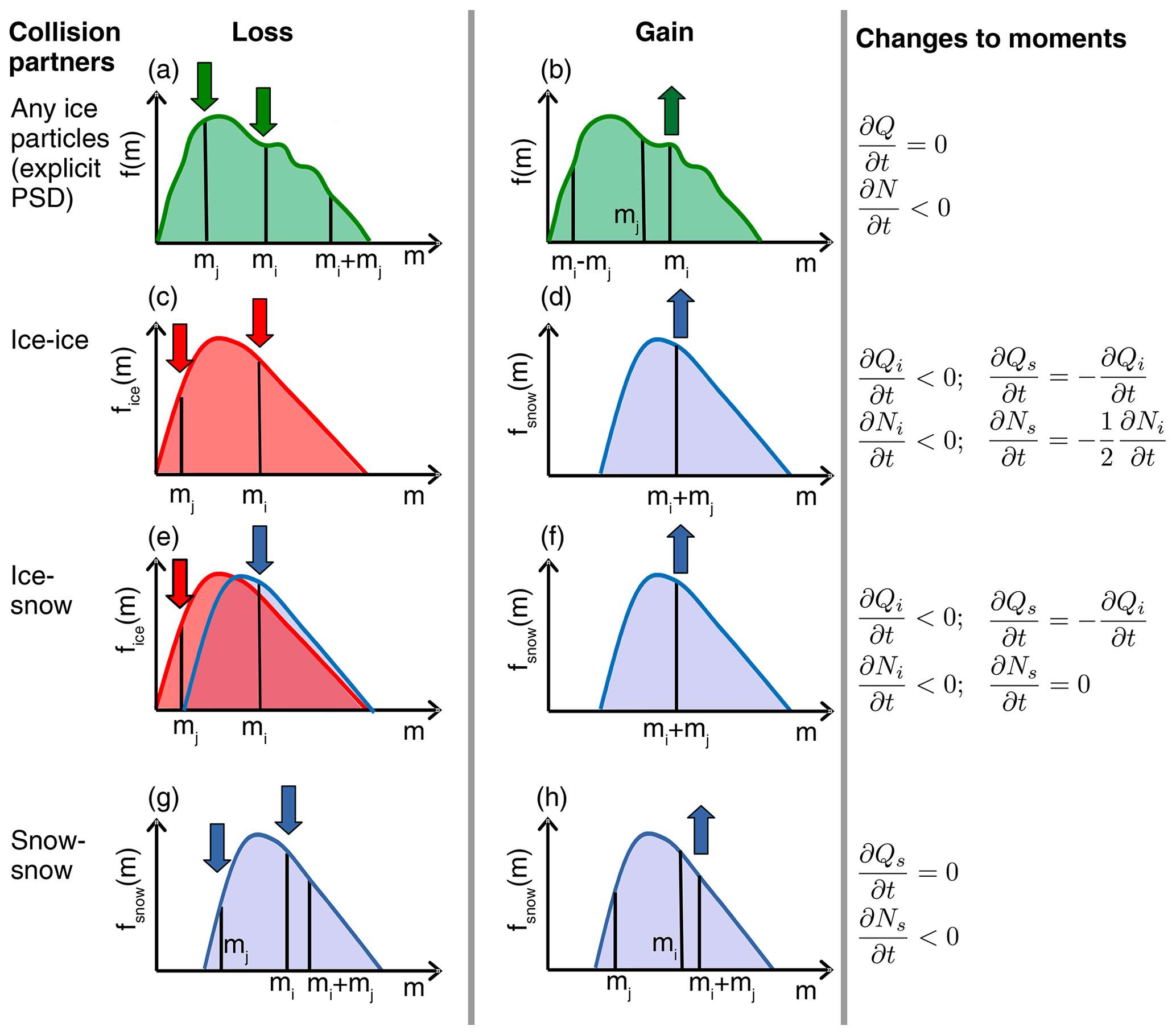
Figure 1Illustration of the SCE (Eq. 4) for an explicitly resolved PSDm (a, b) and when applied to the cloud ice and snow classes of the SB06 scheme (c, h). The left column depicts the loss term (second term in Eq. 4) and the middle column the gain term (first term in Eq. 4). The right column shows the sign and connection of the tendency of the bulk moments. Arrows indicate whether the number density is rising or falling at the specified mass. Red lines indicate the ice distribution and blue the snow distribution. The arrows are red if ice particles are collected and blue if snow particles are collected or are created as a result of the collision.
3.1.1 Size distribution
In most bulk schemes, the PSD is described by the generalized gamma distribution or simplifications thereof. With the mass m as a primary variable, the generalized gamma distribution can be written as
For some applications, using the mass-equivalent diameter
as a primary variable and the ordinary gamma distribution is more convenient:
where Deq is the mass-equivalent diameter. One such application is the use of the Atlas-type vt–size relationship (Eq. 11) in the calculation of collision rates in Appendix A. Size distributions derived from in situ observations are usually presented as a function of the maximum dimension Dmax, which is often derived by circumscribing a sphere or spheroid to the projected particle image.
In general, a distribution described by Eq. (5) cannot be expressed by Eq. (7) or (8). Only when can Eq. (5) be expressed by Eq. (7). To allow conversion of Eq. (5) to (8), μm must be set to (exponent in the m–Dmax relation; Eq. 12). As we calculate the collision rates of particles following an Atlas-type vt–size relation (Appendix A), we need to set . Since bm≠3 for cloud ice and snow, μmax in Eq. (8) can only be approximated.
The PSD shape can vary strongly, e.g., for nonstationary events (Seifert, 2008). Furthermore, νm, or equivalent parameters in distributions that use a different primary variable, is often described as a function of other parameters (e.g., the mean size; Heymsfield, 2003). Nevertheless, in the current version of the SB06 scheme, we must choose a single value of νm in each simulation. Therefore, we test two different values of νm in the simulations and later (Sect. 3.2) select the one with which the simulations can reproduce the observations the best. The SB06 standard configuration (νm=0) corresponds to μeq=2.0 and . If we use νm=2 instead of νm=0, we obtain a narrower distribution with much fewer particles at small masses and a peak near the mean mass. Considering Heymsfield (2003), νm=0 is representative of a mean mass diameter Dmean of about 0.5 mm, and νm=2 is representative for Dmean of about 0.2 mm. Many studies have shown that the size distribution parameters are correlated (e.g., Field et al., 2005; Mcfarquhar et al., 2015), further complicating the selection of νm. Moreover, PSDs can exhibit bimodalities, e.g., due to secondary ice generation (Korolev and Leisner, 2020), which can be accounted for by the two classes of cloud ice and snow in the SB06 scheme.
Table 1Size distribution parameter for , the mass–size relationship of the Mix2 particles (Table 2), kg m−3, and N=104 m4 (same as Fig. 2). ZeKa, MDVKa, and DWRX,Ka are calculated using the self-similar Rayleigh–Gans approximation (SSRGA) and the SSRGA parameters of Mix2 as provided by Ori et al. (2021). μmax is estimated by the zeroth, third, and sixth moment of the distribution.
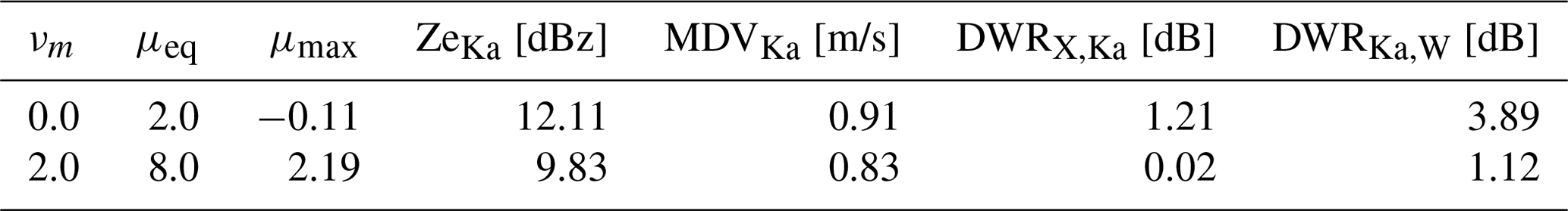

Figure 2Particle distribution as a function of mass (PSDm) with a mass density of kg m−3 and a number density of qn=104 m−3 illustrating PSDs with a different shape parameter μm.
The PSD width affects the aggregation rates and the radar variables. The narrower the distribution is, the lower the aggregation rates are. This is obvious from the bulk collision rates in Appendix A and can be explained by the small vt difference of similarly sized particles (Sect. 3.1.2). The PSD width also affects the radar observables. The reflectivity in the Rayleigh regime is proportional to the second moment of the PSD. A narrower distribution reduces the number of large particles (above 10−7 kg in Fig. 2). Therefore, the reflectivity (Ze) and mean Doppler velocity (MDV) are slightly lower for a narrower distribution compared to a broader distribution with the same Q and N. This effect is even stronger for DWRs, as the large particles contribute the most to the differential scattering signal (Table 1).
3.1.2 Collision kernel
The D-kernel (Eq. 1), defined analogously to the collisional coalescence of droplets in liquid clouds, is often used not only for particles that can be approximated well by spheres (e.g., cloud droplets, hail), but for all particles. However, the collision cross section of nonspherical particles is smaller than the one of spheres with the same Dmax because of the presence of voids in their circumscribing sphere. This deviation was previously considered, e.g., a part of Ecoll (Keith and Saunders, 1989; Pruppacher and Klett, 2010) by using the equivalent circular radii as a characteristic length. Using the D-kernel with a constant Ecoll that does not depend on particle size (as done, e.g., in SB06), the D-kernel approximation cannot account for the decrease in Ar with increasing size (Fig. 3d). Therefore, we test whether an alternative formulation of the collision kernel that takes the projected areas into account (A-kernel; Connolly et al., 2012) provides a better approximation.
The A-kernel approximation has been used previously in the same or similar formulation (Kienast-Sjögren et al., 2013; Morrison and Milbrandt, 2015; Dunnavan, 2021). In these studies, the aggregation rates are calculated numerically and, in the case of the scheme proposed by Morrison and Milbrandt (2015), stored in lookup tables that are used at the model run time. Lookup tables can accurately store precomputed process rates and might be numerically more efficient than analytical solutions, depending on the computer architecture, size of the lookup table, and complexity of the analytical solution. However, Seifert et al. (2014) argue that the use of lookup tables also has disadvantages, like increasing complexity during preprocessing, additional memory access, and difficult reproducibility for follow-up studies. To avoid these disadvantages, the SB06 scheme uses analytical solutions of the variance approximation introduced by Seifert and Beheng (2006). To use the A-kernel we have to generalize the collision rates. For brevity, we moved the lengthy derivations to Appendix A. To our knowledge, this is the first application of an A-kernel in a bulk microphysics scheme that uses an analytical formulation of the aggregation rates. How large the difference is between the D- and the A-kernel depends on the particle properties (e.g., area–size and vt–size relation).
3.1.3 Particle properties
Particle properties influence aggregation because they are an essential part of the aggregation kernel. According to Eqs. (1) and (9) collection is enhanced if the product of the difference in vt and the joint cross section is large. Thus, a particle population will aggregate rapidly if the mean mass is relatively large and particles with largely different vt are present. The coefficients of area–size and vt–size relations of the SB06 default scheme and the particle from K20 are included in Table 2.
While the particle properties of the SB06 default scheme particle classes are taken from in situ observations, K20 used an aggregation model and hydrodynamic theory to simulate the particle properties. The advantages of this approach are that particle properties can be studied over a large size range, are physically consistent, and can be studied in great detail. Particle property relations from in situ observations have a comparably small sample size. Thus, extrapolation to small and large sizes is unavoidable because microphysics schemes need information about particle properties in a large size range. This extrapolation might lead to inaccuracies, such as the overestimation of vt at large sizes (K20). Since we take all snow particle properties (m–size, A–size, vt–size; Table 2) from the same aggregate type within the dataset, all properties are physically consistent. By comparing with in situ observations, K20 found that their mixed aggregates consisting of small columns and large dendrites (Mix2) can approximate mean aggregate properties well. Besides aggregates (including aggregates of columns and aggregates of dendrites; Sect. 3.1.5), K20 also summarized different monomer particle properties, e.g., the columns and needles shown in Fig. 3.
vt of the default cloud ice and snow class increases continuously with increasing size (Fig. 3) due to the power-law relation used.
Due to this continuous increase, the self-collection rates of these hydrometeor classes stay relatively large at large sizes (Figs. B3 and B4). In contrast, the asymptotic approach to a limit of vt in the new relations leads to rapidly decreasing collision rates at large sizes. The asymptotic approach is evident from in situ observations and can be accounted for by using an Atlas-type vt–size relation.
The relative vt of cloud ice and snow particles also plays a role in ice–snow collection rates. In the SB06 default scheme, vt of cloud ice and vt of snow differ greatly. However, K20 showed that vt of cloud ice and snow should have similar values. The difference between cloud ice and snow vt determines the location and magnitude of the minimum of the collection rates.
The projected area A is derived differently in the D- and the A-kernel. In the D-kernel, the m–Dmax relation,
determines the relation between A and size. Since m is the primary variable in the SB06 scheme, it is most useful to consider the differences between the kernels and the particle classes as a function of Deq (which is directly related to the mass).
Thus, the particles which have the lowest effective density,
have the largest A for a given Deq (e.g., needles of K20 in Fig. 3b). The other particles have similar A. In the A-kernel, the actual projected area Aact derived from the particle shape is relevant.
The particle shapes and thus Aact are not defined for the SB06 default classes because this property is not required. The area ratio Ar is commonly defined as the ratio of Aact to the area of a sphere with diameter Dmax.
At small sizes, Ar is close to 1, indicating compact particles and small differences between the D- and the A-kernel (Fig. 3d). With increasing size, Ar decreases down to 0.2 at Deq=5 mm for the Mix2 class and lower for the cloud ice classes needle and column. Aact is similar to observations of Mitchell (1996) as shown in K20.
However, the low values of Ar of the cloud ice classes are less important because such large sizes of cloud ice are rarely reached in the model. The decrease in Ar leads to a decrease in collision rates, especially at large sizes, similar to the Atlas-type vt–size relations. Thus, combining the new vt–size relations with the A-kernel substantially decreases collision rates at large sizes.
While the properties of snow can be validated well against mean observed quantities (as done in K20 and in Sect. 3.1.5 of this study), selecting a single habit for cloud ice is a strong simplification that is necessary for a simplified microphysics scheme.
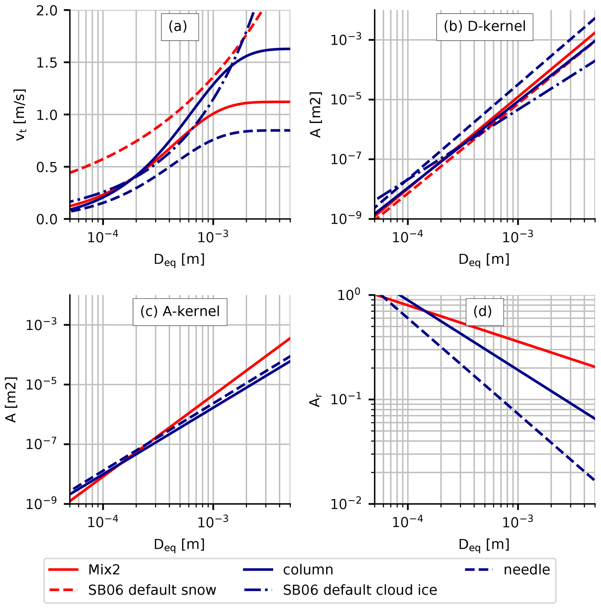
Figure 3Particle properties from the default (SB06 default cloud ice, SB06 default snow) and modified version (column, needle, Mix2) of the scheme. (a) Terminal velocity vt, (b) projected area A of a circumscribing sphere (as assumed in D-kernel), (c) “real” projected area A considering the voids in the circumscribing sphere (as assumed in A-kernel), and (d) area ratio (Eq. 16). The default scheme does not assume an A–D relation explicitly, and therefore the real projected area and the area ratio are not given.
Table 2Parameterizations used in ICON-LEM, the snowshaft model, and radar forward simulations of hydrometeor properties in PAMTRA. D represents the particle maximum dimension and the mass-equivalent diameter; m is the particle mass and ρw the density of water. The mass–size (m–D), terminal velocity vt–size, and projected area–size (A–D) relations are reported in their full mathematical form. For the SSRGA scattering model, the four parameters (κ, β, γ, ζ0) are given in parentheses. SB indicates that the properties are exclusively used in the default setup. Cloud droplets, rain, graupel, and hail (which are only relevant for the 3D simulations) follow the same properties in all simulations. The aspect ratio is 1.0 for all classes except for the snow classes (SB snow, Mix2, and Mix2; O20 scat), for which an aspect ratio of 0.6 is assumed. All variables are in SI units.

3.1.4 Sticking efficiency
The parameters discussed so far determine how often collisions occur. The percentage of the colliding particles that stick together after a collision is defined by the sticking efficiency Estick.

Figure 4The sticking efficiency (Estick) in the SB06 scheme for collisions among ice particles (ice self-collection) follows L83; for other collisions (ice–snow collection, snow self-collection) it applies the C86 parameterization. Our new relation (red) combines the relations from M88 and C12 with a characteristic maximum around −15∘ C and values quickly approaching unity for temperature larger than −5∘ C.
Estick is mostly only described as a function of the temperature (Mitchell, 1988; Connolly et al., 2012, M88, C12). To stick to each other, ice particles must form ice bonds (Lamb and Verlinde, 2011), which is highly unlikely for colliding solid-ice particles when the temperature is well below the melting temperature and the particles only touch for a short time. There are two main mechanisms that increase the likelihood of adhesion after a collision and explain the temperature dependence. The first mechanism is explained by the quasi-liquid layer (QLL) on the ice particle surface. The phenomenon of QLL has been studied since the mid-19th century (Slater and Michaelides, 2019). QLL thickens with increasing temperature and consists of weakly bound molecules on the particle surface (Slater and Michaelides, 2019). When two particles touch, the molecules form a solid bond at the point of contact. The second mechanism is the mechanical interlocking of relatively large particles with dendritic features (Pruppacher et al., 1998). These dendritic features occur at temperatures between −17 and −12 ∘C.
The SB06 default scheme uses the Estick parameterization of Cotton et al. (1982) for ice–ice collisions and Lin et al. (1983) for ice–snow and snow–snow collisions (Fig. 4). The exponential shape of both parameterizations can be justified by the approximately exponentially increasing QLL thickness. These relations, however, miss the maximum of Estick suggested by studies (M88, C12) that consider the mechanical interlocking mechanism.
We combine M88 and C12 to propose a new parametrization. For ∘C we follow C12, then linearly approach the plateau proposed by M88 with Estick=1 between −17 and −12 ∘C. As discussed in the Introduction, there is ample evidence from both in situ and remote sensing observations that Estick is likely to be present at temperatures near −15 ∘C (at which particles with dendritic features are present) and near the melt boundary. At −10 ∘C the new parameterization again follows C12 but increases towards 1 at higher temperatures, at which C12 does not provide an estimate of Estick. One might prefer to follow C12 rather than M88, since C12 derived Estick directly from laboratory measurements and M88 provided only an ad hoc parameterization. However, C12 analyzed only the initial stage of aggregation, during which few monomers compose the aggregates. The interlocking mechanism might be more efficient for more complex aggregates compared to early aggregates as discussed in C12. Even considering only the initial stage of aggregation, the confidence interval of Estick at −15 ∘C ranges from 0.35 to 0.85 (C12).
3.1.5 Selecting a particle type representative for a large aggregate ensemble
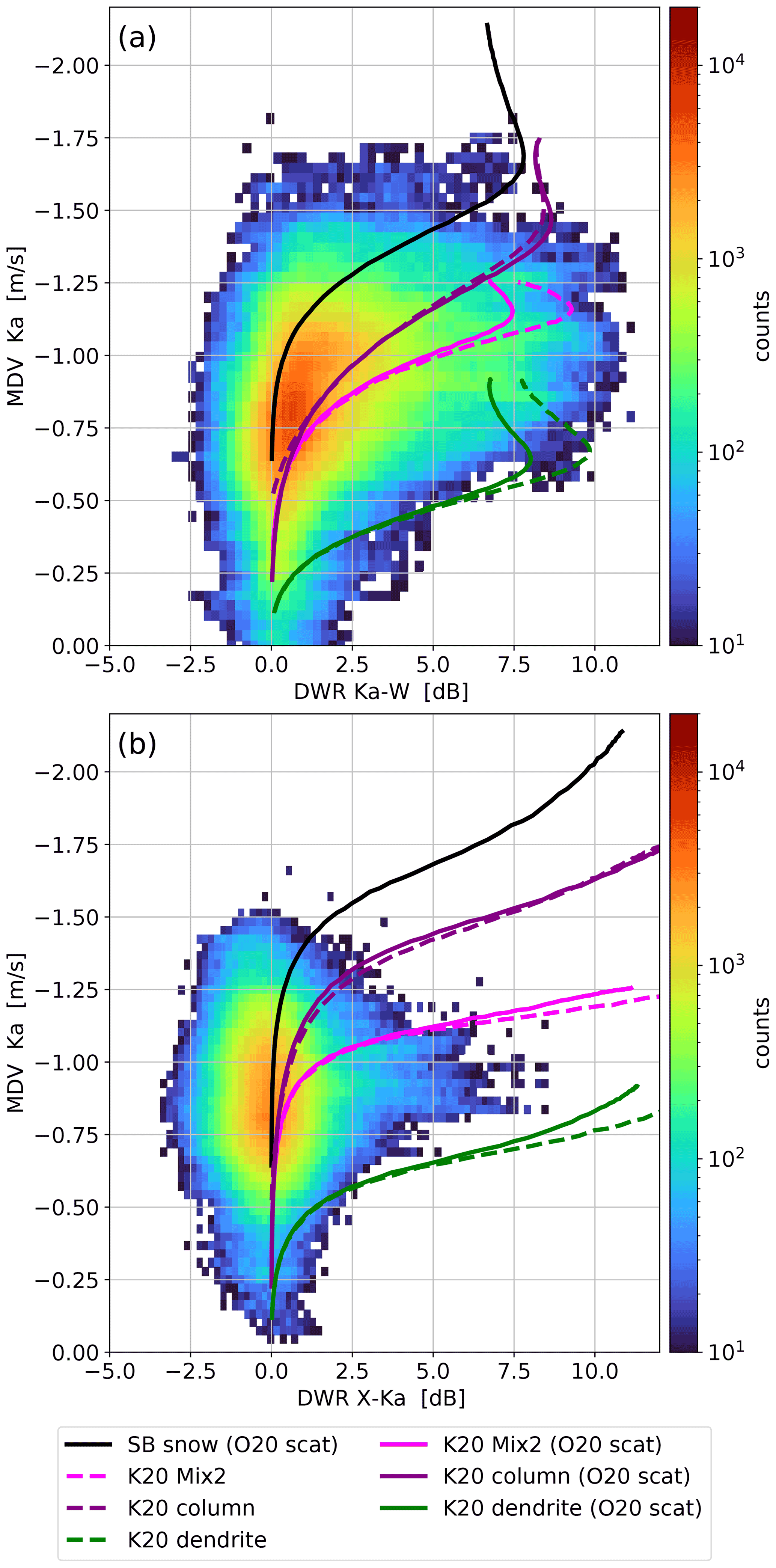
Figure 5Comparison of the modeled and observed relationship between MDV and DWR: (a) DWRKa,W, (b) DWRX,Ka. The histogram shows the observations from the Tripex campaign (D18). The lines show the theoretical MDV at a given DWR for the vt size relations of snow particles as assumed in the SB default (black) and as modeled in K20. For the dashed lines, the SSRGA parameters have been directly derived from the corresponding aggregate ensemble properties (as found in Ori et al., 2021). The solid lines use SSRGA parameters as used in O20 in order to illustrate the uncertainty due to the scattering parameters. The lines are calculated using PAMTRA and the properties of the US standard winter atmosphere at 700 hPa.
After discussing the various components of the aggregation process formulation, we need to decide which aggregate type to use to best represent the physical particle properties (e.g., vt) and scattering properties. In O20, the particle properties were defined by the assumptions in the standard SB06 scheme. The best-fitting aggregate model and associated SSRGA parameters were selected based on the best fit in the triple-frequency DWR space. In this section, we ask whether there is an aggregate type in the database of K20 and Ori et al. (2021) that reproduces both the physical and scattering properties well compared to the observations.
O20 already noted that the representation of MDV as a function of DWR resembles to some extent the underlying vt–size relation. In contrast to the triple-frequency DWR-DWR, the MDV-DWR space is rather insensitive to the PSD width. Different aggregate types composed of different monomer types generated and studied in K20 are used to simulate their corresponding MDV-DWR signatures (Fig. 5). The underlying distribution shows the observed values from D18, which naturally contain larger scatter and even negative DWR values, mainly due to imperfect radar volume matching (for a detailed discussion, see D18). Fortunately, as shown in D18, the dataset contains only very short and weak riming events. This scarcity of substantial riming is important because the increased MDV due to riming would bias our comparison. Moderately or strongly rimed particles would exceed 1.5 m s−1 upon reaching a size that results in a nonzero DWRKa,W (Mason et al., 2018). The MDV-DWR space is also well-suited to evaluate our aggregate choice, as it combines the two radar variables that showed the largest discrepancies with the model simulations in O20.
O20 already recognized the overestimation of vt at large sizes, which is also evident in Fig. 5. For example, at DWRX,Ka=5 dB the observed MDV scatters around 1 m s−1, while the snow falls at 1.7 m s−1 in the SB06 default scheme. From the aggregate dataset of K20 the aggregates of dendrites fall the slowest and the aggregates of columns fall the fastest. A mixture composed of small columns and large dendrites (Mix2), which fit in situ observations (K20) best, also matches the observations in the MDV-DWR space well. Therefore, we utilize the Mix2 aggregate properties as an improved description for the snow class in the following.
Interestingly, the use of the SSRGA coefficients of the aggregate type O20 does not lead to a strong change in the curves in the MDV-DWR space. Although it would be most consistent to use the SSRGA coefficients of Mix2 directly, we will use the scattering properties of O20 in the following analysis to allow a fair comparison of our new results with the discrepancies found in O20.
3.2 Exploring sensitivity to microphysical parameters in the snowshaft model
The snowshaft model (Sect. 2.1) allows us to test the influence of the particle properties, the formulation of the collision kernel, Estick, and the size distribution on the aggregation rates with low computational effort and with reduced complexity. In Sect. 3.1 we showed how these parameters affect aggregation. We not only examine the influence of the parameters on the predicted model variables but also on the radar observables. After carefully setting up the model, the comparison in radar space enables us to directly contrast the statistics of the simulation and the observations, as given in O20 and D18. Since we compare the statistics of the model and observations over a relatively long time range this analysis already attempts to select a combination of parameters that can reproduce the observational statistics well. The optimal parameter combinations found in the snowshaft simulations will then be applied in the 3D model to simulate a case study (Sect. 3.3) before we use it to rerun simulations for the whole time period of the Tripex campaign (Sect. 3.4).
This comparison between the model and observation benefits from the simultaneous consideration of multiple model parameters and multiple observables. When looking at a single observable only, one might reduce a bias by an adjustment of a single process or parameter, even though this might just compensate for an inaccurate choice in another parameter, introducing compensating errors. As the number of independent observables increases, this problem is reduced as the inaccurate choice of a parameter might be detectable in one of the remaining observables. In other words, the larger degree of freedom in the observations helps to better constrain the parameters by comparison with the model when several observables are considered. We focus our comparison on the DWRs (as a measure of particle size) and the MDV (as a measure of vt). These two quantities constrain the strength of aggregation and the assumed vt–size relationship, and the statistical comparison in O20 also revealed the largest differences between observations and the model in these variables.
3.2.1 Optimizing the snowshaft model and selecting microphysical parameters for new setup
O20 pointed out that the inconsistencies between observed and synthetic MDV and DWRs are especially evident for raining periods. As we attempt to remove these inconsistencies, the atmospheric variables and the hydrometeor contents at the top of the simulation are chosen so that the hydrometeor profiles in the snowshaft simulation roughly follow the profiles of the ICON-LEM simulations from O20 wherein RR is larger than 1 mm h−1; compare “default” and the histogram in Fig. 6. To match the profiles the RHi has to be set to 1 % above about −18 ∘C with increasing values up to about 6 % at about −7 ∘C. These values of RHi, which are relatively high compared to those from the ICON-LEM simulations (Fig. B5), might be necessary because of the absence of nucleation and advection in the snowshaft simulations. Also, the values of Qi, Ni, Qs, and Ns at the model top are chosen so that the hydrometeor profiles of the CTRL simulation (performed with the SB06 default setup) match those of the profiles of the ICON-LEM simulations of O20 with RR > 1 mm (Fig. 6). After this optimization of the snowshaft model, the simulated profiles from ICON-LEM (O20 and Figs. 11 and 12) and the snowshaft model (Figs. 6) reveal that a simple initialization (nucleation) of the profiles at cloud top is sufficient at least for testing the sensitivities of aggregation to our set of parameters and various formulations.
After iterating over many parameter combinations, we found one particular setup (which we refer to as colMix2_Akernel or simply as NEW) to match the observed profiles particularly well. In these iterations, we varied mostly the less-known components, e.g., the size distribution width, while parameters that we were already better able to constrain (Sect. 3.1.5), e.g., the vt size relation, were not varied. Our approach can hence be seen as a combination of a purely physically based approach, incorporating current knowledge of parameters obtained, e.g., through laboratory studies, and an empirical correction based on observations.
3.2.2 Sensitivity of aggregation to individual ice microphysical parameters in the snowshaft model
The hydrometeor profiles (Fig. 6) and radar observables (Fig. 7) of the NEW setup exhibit many interesting differences from the profiles of the CTRL run. In the following, we discuss where the differences originate from by looking at the different sensitivity runs. In each sensitivity run only one set of parameters is different from the NEW run (Table 3).
The cloud ice mixing ratio Qi and the cloud ice number density Ni are lower in the NEW run than in the CTRL run for ∘C (Fig. 6). At the same time, the snow mixing ratio Qs and number density Ns are slightly larger in the NEW run at temperatures below −17 ∘C. These differences can be explained by the higher Estick at lower temperatures in the NEW setup (Fig. 4), which leads to more collisions among cloud ice particles, and therefore more particles are converted from the cloud ice to the snow category. When using the Estick parameterization of Cotton et al. (1982) and Lin et al. (1983) (colMix2_Akernel_LinCot;), Qi and Ni are larger at lower temperatures (and Qs and Ns are smaller).
The smaller values of Estick in colMix2_Akernel_LinCot compared to NEW at lower temperatures (compare L83 and C86 with “new” in Fig. 4) lead to further differences; colMix2_Akernel_LinCot has a smaller mean mass , which is the mean mass of the sum of the cloud ice and snow class (), and correspondingly lower DWRs for ∘C (Fig. 7c and d). The smaller mean size also leads to slower-falling particles (visible in MDV; Fig. 7b). For ∘C the strong increase in Estick in colMix2_Akernel_LinCot triggers a strong increase in and DWRX,Ka. A similar increase in the mean and median of the investigated statistics of DWRX,Ka was already discussed in O20. As in O20 the strong increase is not visible in DWRKa,W, since this observable already reaches saturation for mass median diameters of about 3 mm (Sect. 2.5). The local maximum of the new Estick parameterization at temperatures from −17 to −12.5 ∘C leads in the NEW run to a rapid increase in the , DWRs, and MDVs in the same temperature range and therefore matches the observed profile of DWRKa,W better than the CTRL run.
O20 speculated that the overestimation of the particle sizes at high temperatures and the mismatch in the profiles of the DWRs might be mainly due to the Estick parameterization and the vt–size relation. However, Figs. 6 and 7 as well as the aggregation rates (Appendix A) reveal that the vt relation at smaller sizes and the aggregation kernel formulation also strongly affect the aggregation rates. Both (Fig. 6i) and DWRX,Ka are lower in colMix2_Akernel_LinCot than in the CTRL run. If Estick were the dominating driver, these two simulations would be very similar. The differences in the profiles of these two simulations can only be explained by relevant influences of other parameters on the aggregation rates. The simulations with the D-kernel (colMix2_Dkernel) exhibit a strong influence on aggregation. This is evident in the rapid decrease in Qi and Ni and a rapid increase in , , and caused by high aggregation rates (supported by Appendix A). From this simulation, it is evident that the use of the new particle properties (including the Atlas-type vt–size relation) together with the D-kernel results in even larger particles than in the default run, and thus DWRs are strongly overestimated (Fig. 7d). This overestimation can only be reduced by using the A-kernel.
The vertical gradients of Q result from mass uptake by depositional growth and divergence of vt (Fig. 6h). First, Q increases from the cloud top to the cloud bottom due to depositional growth. Second, deposition growth and aggregation increase particle size and thus vt increases. If there were no mass uptake (no deposit growth) but only aggregation, Q could only decrease because the product of vt and Q would be conserved. The vt–size relation plays an important role in these processes: on the one hand, smaller vt for a given particle size, e.g., as in NEW vs. CTRL, means more time for mass uptake, leading to a faster increase in Q per height. On the other hand, smaller vt could also lead to less ventilation and thus less mass uptake due to depositional growth. The vt–size relationship, which defines the slope of vt with increasing size, influences the divergence of vt with height and the aggregation rates (Sect. 3.1.3). These multiple effects also interact, which further complicates the interpretation of the profiles of Q. Nevertheless, we attempt to interpret the most obvious features of the profiles of Q.
At about −17 ∘C, MDV increases sharply in the NEW run (Fig. 7b), causing a decrease in Q at these temperatures (Fig. 6f), while Q increases continuously in the CTRL run. The differences in the profiles of Q between the sensitivity runs are relatively large. These large differences are likely due to the different conversion rates of cloud ice to snow and differently strong increasing near the model top. For example, in colMix2_Dkernel the cloud ice converts rapidly to larger snow particles. As a result, particles near the model top fall faster and therefore have less time to grow by depositional growth (the increase in Q is weaker compared to the NEW run); colMix2_Akernel_LinCot shows a weaker increase in for 15 ∘C compared to the NEW run (Fig. 6i). This weaker increase in leads to a weaker increase in MDV (Fig. 7b) and thus to a stronger increase in Q (Fig. 6h). The reflectivity ZeKa is closely related to Q so that colMix2_Dkernel (colMix2_Akernel_LinCot) has the lowest (highest) reflectivity. However, the CTRL run has the highest ZeKa, although Q is lower than in some sensitivity runs. The large ZeKa here could be caused by the relatively dense snow particles assumed in CTRL (Fig. 3). Overall, Q and ZeKa show relatively large sensitivity to the varied parameters in these snowshaft simulations. However, this observation must be interpreted with caution. The simulations assume a relatively large humidity in order to match the hydrometeor profiles and compensate for processes not considered (Sect. 3.2.1). This high humidity could lead to an overestimation of mass uptake due to depositional growth. Additionally, considering that supersaturation is not consumed by depositional growth but is held constant in our snowshaft simulations, one could hypothesize that Q and Ze might be more similar among the sensitivity runs in the ICON-LEM simulations.
The new particle properties reduce the bias of the scheme regarding MDV to a large extent (Fig. 7b). While all simulations with the new particle properties are within the deciles of the observations, the standard run is already outside the deciles at −35 ∘C and is more than 0.5 m s−1 larger than the median at some temperatures (e.g., at T=5 ∘C). The other parameters change the profile of the MDV to a much lesser extent. At temperatures from −18 to −12 ∘C, all simulations show an increase in MDV, while all quantiles of the observed MDV decrease. This discrepancy could be due to the lack of habit prediction, underestimated or missing upwinds, or the lack of collisional fragmentation (Korolev and Leisner, 2020) in the model. At these temperatures dendritic growth occurs, which could lead to decreasing particle density and thus decreasing vt and/or updrafts as a result of strong latent heat release. Collisional fragmentation could furthermore lead to the formation of new small particles with low vt, which also reduces the MDV.
In addition to the particle properties, the width of the size distribution changes the MDV the most. The simulation with the wider size distribution (colMix2broad_Akernel) has a larger MDV (Fig. 7b) than the NEW run, which is due to the increasing number of large particles at the larger end of the distribution (Sect. 3.1.1). These large particles contribute more to the MDV than the smaller particles; to calculate MDV, each particle must be weighted by reflectivity, which for Rayleigh scatterers scales approximately with mass to the power of 2. The higher weight of the large participants also explains why the DWRs in colMix2broad_Akernel are significantly higher compared to the NEW run, even though the mean size of the hydrometeors is relatively similar. This sensitivity illustrates that the DWRs can only to some extent be used to infer and the size distribution width has to be additionally considered.
Despite the various simplifications in the snowshaft model (no nucleation, no advection, constant humidity) the mean profile of the radar profiles from the ICON-LEM simulations of O20 could be well-matched. This allowed us to investigate the sensitivity of aggregation to the individual model components and to select a model setup that best matches the observed radar profiles. The particle properties of the snow, the aggregation kernel formulation, and Estick have a strong influence on the hydrometeor contents and the simulated radar observables. Interestingly, the choice of particle size distribution has little effect on the hydrometeor profiles but a large effect on the DWR values. The choice of cloud ice properties (needle or column) is less important than the choice of the other parameters in this cloud regime. However, the choice of cloud ice properties might be more important for clouds with smaller aggregation rates, e.g., cirrus. If we combine the A-kernel, the particle properties of Mix2 from K20, the newly proposed Estick parameterization, and a relatively narrow size distribution the observed profiles of MDV and DWRs could be better matched. To test whether these sensitivities and improvements in NEW are also found persistently in more realistic simulations, in the next section we test whether these observations occur similarly in the ICON-LEM simulations.
Table 3Overview of parameters and settings varied in the microphysical sensitivity experiments. The sensitivity runs have the same settings as colMix2_Akernel unless otherwise noted. K is the collision kernel, D the maximum dimension, and A the particle's projected area; μ and ν are parameters in the generalized gamma function describing the mass distribution in the microphysics scheme (Eq. 5).

.
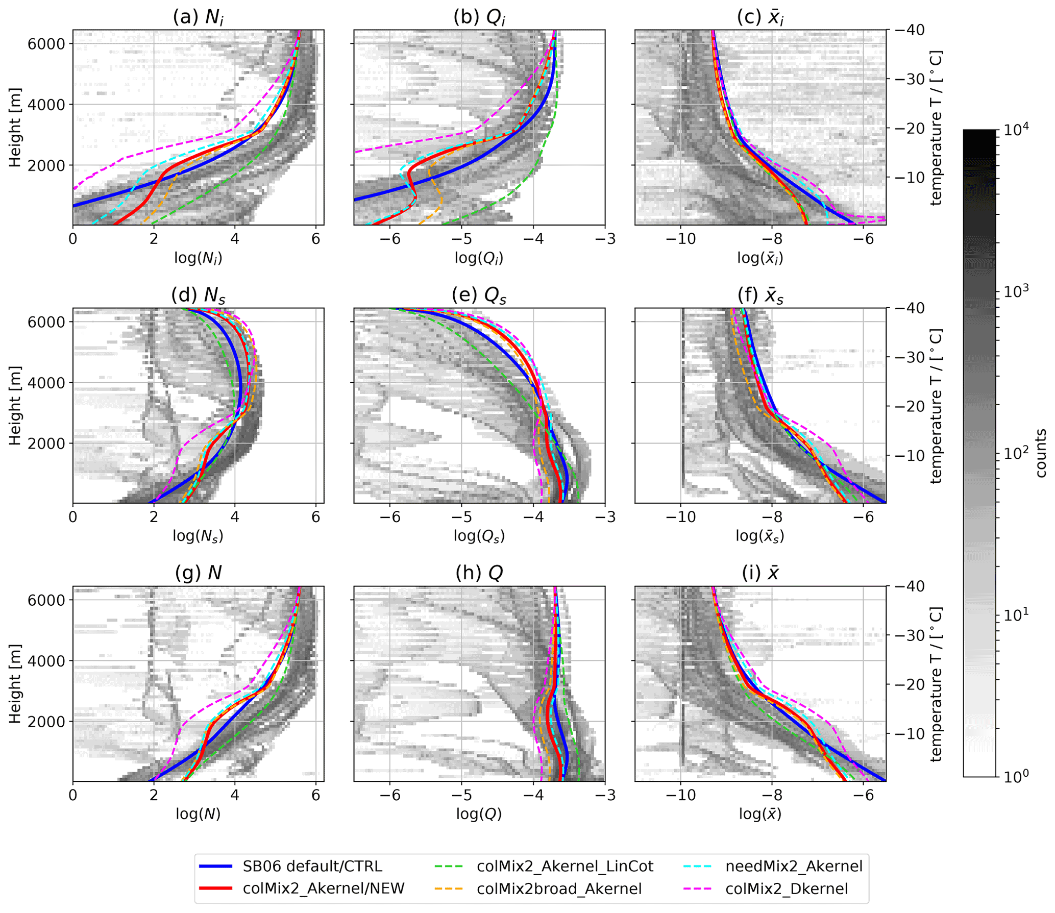
Figure 6Profiles of model variables in the snowshaft simulations. Number density N (a, d, g), mass mixing ratio Q (b, e, h), and mean mass (c, f, i) of the cloud ice (a, b, c), snow (d, e, f), and the sum of cloud ice and snow (g, h, i). Lines: simulations using different model settings as described in Table 3. Greyscale: histogram of the hydrometeor contents vs. temperature from the ICON-LEM simulations of the Tripex campaign (O20) filtered to include only profiles for which the precipitation rate exceeds 1 mm h−1. The simulations in O20 used the default model settings.

3.3 ICON-LEM case study simulation using the new parameterizations
In the snowshaft simulations (Sect. 3.2) we had to use several idealized assumptions. ICON-LEM (Sect. 2.2) contains additional processes (e.g., advection, nucleation, varying humidity field) and therefore simulates a more realistic representation of the atmosphere. In this section, we investigate the impact of the various parameters studied in the sensitivity analysis in a more complex case study with an ICON-LEM simulation. Furthermore, the ICON-LEM simulations provide an opportunity to extend the analysis to various conditions (e.g., nonstationary regime during the frontal passage, sublimation layers).
The case study of interest was 3 January 2016, when a low-pressure area over the British Isles and an accompanying frontal system over western and central Europe determined the synoptic situation over the modeled domain. Shallow mixed-phase clouds are present in the morning and dissipate around noon (Fig. 8a). The passage of a warm front manifests itself at 10:00 UTC, first in high clouds and then in sinking cloud bases. These frontal clouds start to precipitate at 18:00 UTC. The selected case is particularly interesting because it contains clouds in different regimes and precipitation of weak to moderate intensity.
The observed and simulated ZeKa fields match relatively well for all simulations in terms of cloud structure and precipitation (Fig. 8). Both the shallow mixed-phase clouds and the frontal cloud are very well-captured in terms of temporal and spatial structure.
ZeKa exhibits strong differences between the observations and the simulation only in the rain and ice slightly above the melting temperature in the period from 19:00 to 23:00 UTC. The sharp decrease in the observed ZeKa indicates strong sublimation. The presence of sublimation is also revealed by the model showing subsaturated air in this time range (Fig. B6). There are three main reasons that explain why the model does not accurately represent the sharp decrease in ZeKa in this sublimation scenario. First, the humidity could be overestimated in the model, e.g., due to inaccurate forcing data. Second, particle sizes could be overestimated due to processes in microphysics that weaken the effect of sublimation. We cannot completely rule out the humidity mismatch, but we found good agreement between the model and radiosonde data when available. Unfortunately, there was no radiosonde launched on the considered day. Thus, we are confident in the general ability of the model to accurately simulate the humidity field, but we cannot rule out the possibility that inaccuracies in the simulated humidity field contribute to the bias in ZeKa. Lastly, the parameterization of sublimation could also be an error source. For example, the evolution of the PSD during sublimation is challenging to represent in a two-moment scheme (Seifert, 2008). Since all of these reasons might be able to explain the mismatch in ZeKa, we should be cautious in assessing the validity of the assumptions of the individual model settings based on this sublimation feature. However, regardless of the accuracy of the model in predicting the humidity or simulating sublimation, the following differences in ZeKa of the model simulations underscore the importance of accurate prediction.
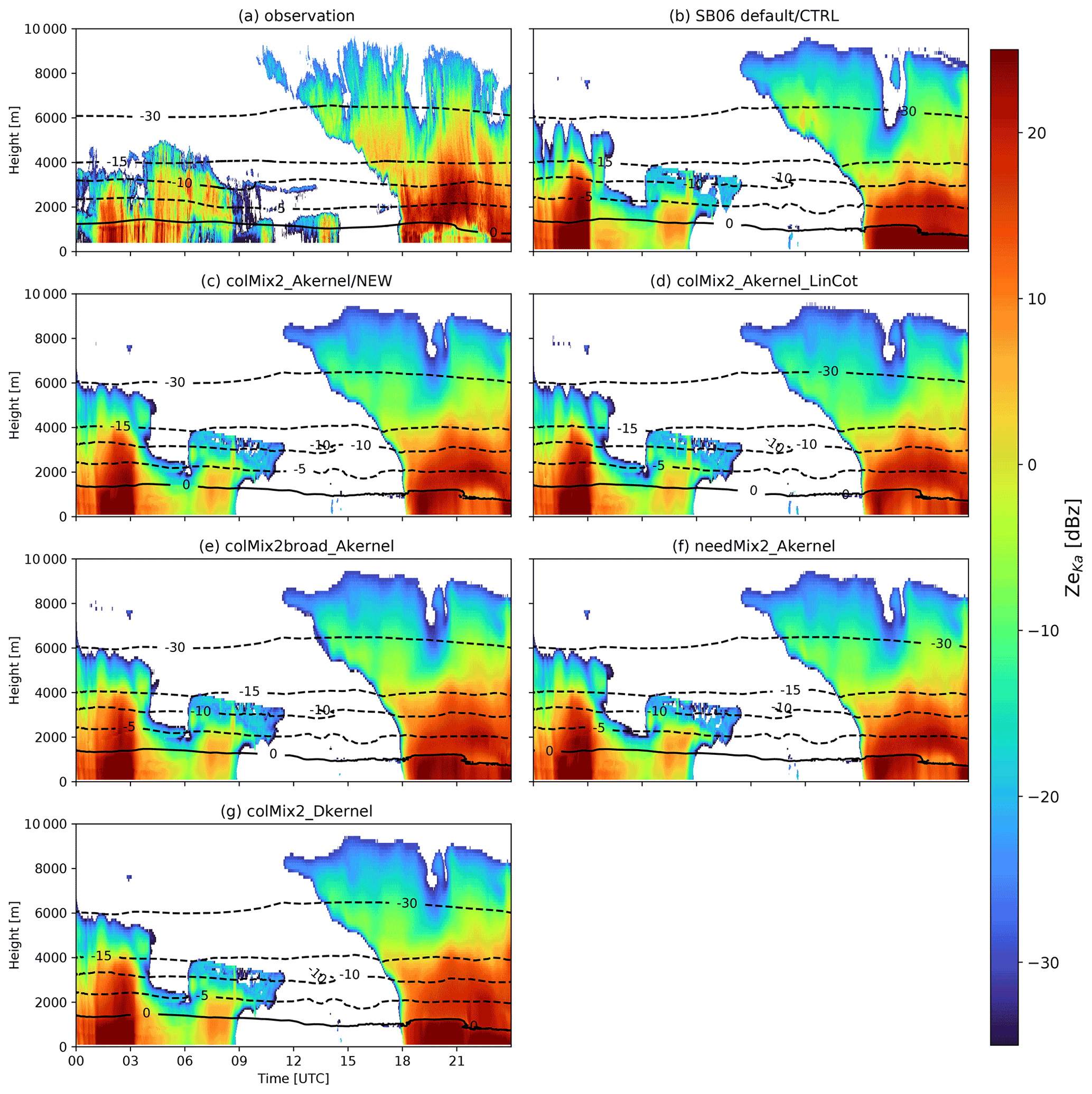
Figure 8Time–height profile of ZeKa from 3 January 2016 as observed (a) and simulated (b–g) with various model settings (Table 3). Selected temperature isolines from CloudNet (Illingworth et al., 2007) for the observations (a) and the corresponding ICON-LEM output (b–g) are also shown.
While the NEW (Fig. 8c) and most sensitivity runs show a slight decrease in ZeKa due to sublimation in the time period when the air is subsaturated, the sublimation is barely seen in ZeKa of some other simulations (e.g., CTRL, colMix2_Dkernel; Fig. 8b and g). The differences between the simulations are caused by the differences in the particle size indicated by DWRX,Ka (Fig. 9). Similar to the snowshaft simulations, DWRX,Ka is strongly overestimated in colMix2_Dkernel and the CTRL run. In contrast, DWRX,Ka is well-matched closely above the melting temperature in the NEW simulation. The hydrometeor populations with realistic particle sizes are more strongly affected by the subsaturated air and sublimate quickly, whereas particles that are too large sublimate less and therefore retain more mass. Thus, the overestimated particle size leads to overestimated precipitation. Between 18:00 and 24:00 UTC, 1.40 mm of accumulated rain was observed, 8.91 mm simulated by the default simulation and 2.29 mm by colMix2_Akernel. While this represents an overestimates of 536 % by the CTRL run during this time period, we emphasize the overall good agreement between modeled and observed precipitation reported by O20 for the entire campaign. While Estick appeared to be important for the simulated DWRKa,W in the snowshaft simulations (Fig. 7), the differences between the simulation with the old (colMix2_Akernel_LinCot; Fig. 9d) and the new Estick parameterization (colMix2_Akernel; Fig. 9c) are relatively small. In the ICON-LEM simulation, the weaker growth of the particles in colMix2_Akernel_LinCot at lower temperatures might be partly compensated for by advection or nucleation.
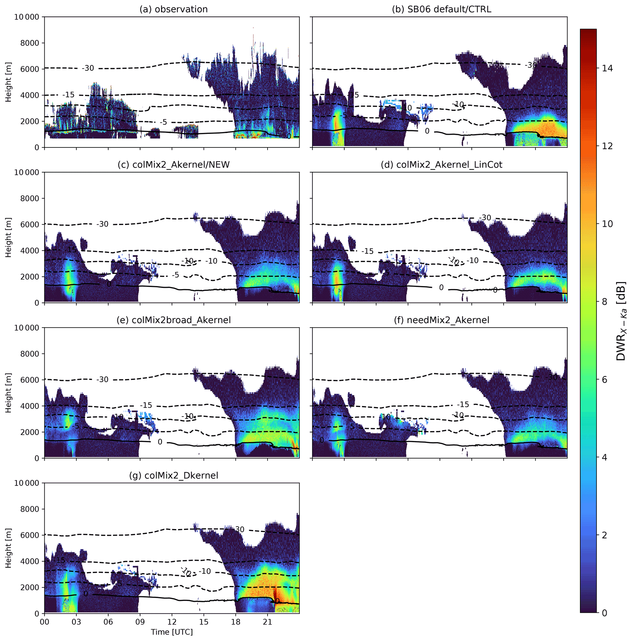
Figure 9Same as Fig. 8 but displaying DWRX,Ka, which is sensitive to mean mass diameters of 1 to 20 mm.
Besides the DWRs, MDV provides valuable information about the microphysical properties. As also reported by O20, MDV is overestimated in the SB06 default simulation, especially in regions where the particle sizes are overestimated (Fig. 10). MDV is often used to distinguish rimed from unrimed particles (e.g., Mosimann, 1995). Using this method, we detect some smaller episodes in which rimed particles dominate at about 04:00, 18:00, and 22:00 UTC. At other times, the observations indicate unrimed or only slightly rimed particles. In the SB06 default simulation, high MDVs are obtained in the whole time range after 18:00. Since the profiles of the hydrometeors show only very little mass of rimed particles during this period, the larger predicted MDV can be attributed to the overestimation of the unrimed snow particle vt.
The new simulations, all using the new particle properties, have significantly lower values of MDV at all temperatures. This reduction of MDV compared to the SB06 default setup constitutes a significant reduction of the bias in MDV at temperatures below −10 ∘C. For ∘C, MDV is even slightly underestimated. Considering that Fig. 5 shows good agreement of MDV between the observations and the vt–size relation of Mix2, we assume that the underestimation of MDV is not caused by the underestimation of the vt–size relation of aggregates. Since DWRX,Ka also matches well at these temperatures, processes other than aggregation and sedimentation of unrimed aggregates most probably cause this underestimation of MDV. One could speculate that riming rates are underestimated or that the vertical air motion is not well-simulated.
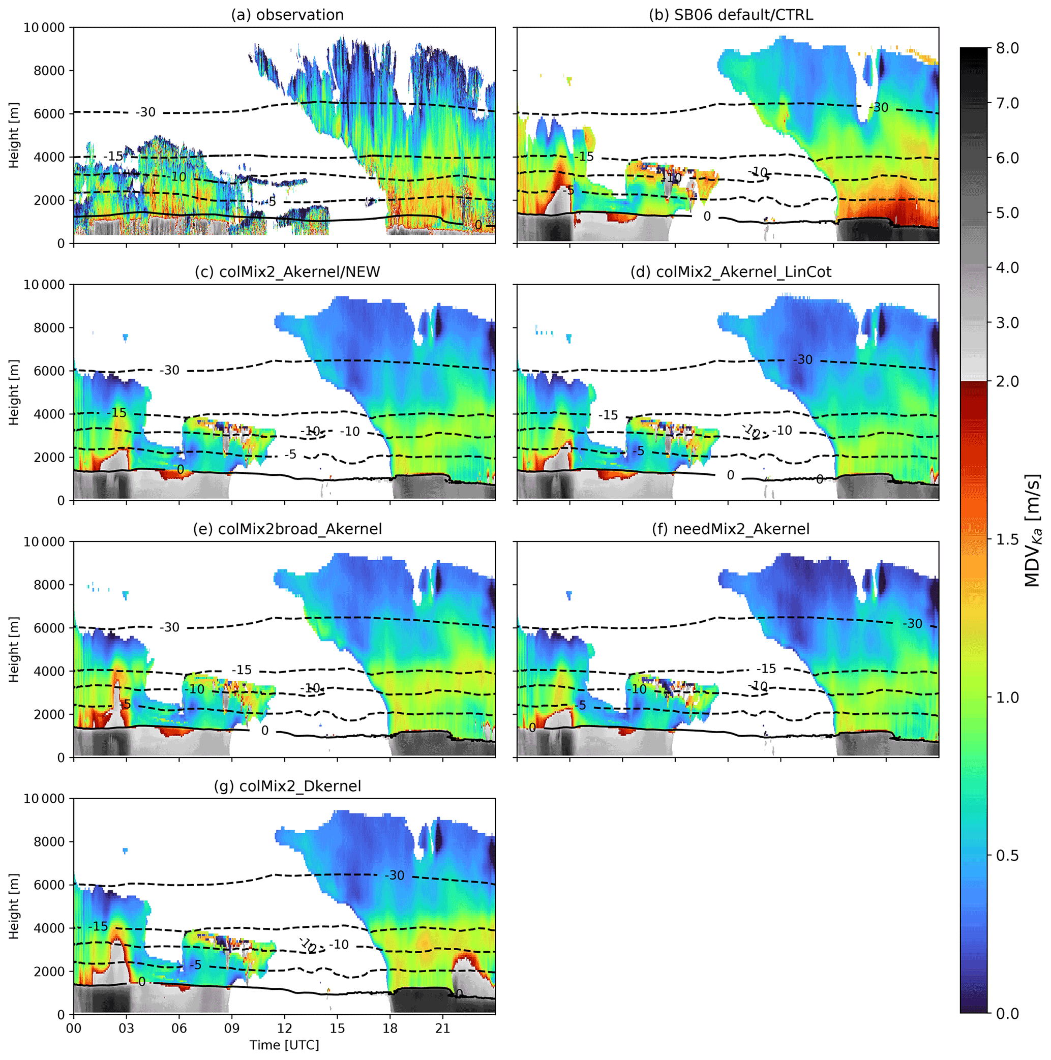
Most of the findings from the snowshaft simulations (e.g., the strong reduction of MDV and DWR at temperatures close to the melting temperature) are confirmed by the ICON-LEM simulation of this case study. However, the ICON-LEM simulations reveal that the influence of Estick seems to be overestimated in the snowshaft simulations. Moreover, accurate modeling of particle sizes and vt in the presence of a sublimating layer is critical. The simulations with the new particle properties showed a slight underestimation of the MDV. This underestimation most likely does not arise from an inaccurate representation of the particle properties or the aggregation rates but is caused by another process (e.g., riming, vertical air motion). In previous analyses of the SB06 default setup, this underestimation could not have been detected because it was masked by the overestimation of the aggregate's vt. Because errors can be specific to the chosen day, such as a particular mismatch of the relative humidity, relying on only one case to detect a discrepancy in the microphysical properties is prone to error. Therefore, we analyze the statistics of a multi-month simulation in the next section.
3.4 Statistical comparison
After evaluating the choices of the new scheme in the snowshaft model and in a case study with ICON-LEM, we perform ICON-LEM simulations for the entire Tripex time period. By comparing observed and modeled histograms of DWR and MDV as a function of temperature, we can evaluate the new scheme. Since we additionally contrast the histograms of the NEW and CTRL simulations, we can test whether the reduction in the bias of DWRs and MDV found in Sect. 3.3 is specific to the selected case or rather a consistent feature of the model changes. As DWRs are related to the mean particle size, we can assess whether the chosen parameter combination can accurately simulate aggregation in various weather situations present in the simulated days. The same applies to MDV profiles, which are especially valuable in evaluating the suitability of the assumed vt–size relationship.
The observed and synthetic radar profiles are filtered in the same way for comparability. For example, the first 6 h of simulation and observation are not considered because the model output could contain artifacts during this spin-up time. Moreover, we include only profiles in which the rain rate RR exceeds 1 mm h−1. The latter filter enables us to focus on the most relevant cases for precipitation. Interestingly, O20 found the discrepancy between the model and observations to be especially obvious for these profiles. For a detailed description of the processing, we refer to O20.
To quantify the agreement between the histograms of the simulations and the observation, the Hellinger distance H is used. H can be defined for two distributions P =(p1, …, pk) and Q =(q1, …, qk) as
H is zero for two identical distributions and 1 if the distributions do not overlap at all.
The medians and larger quantiles of the observed distributions of DWRs indicate a strong increase in particle size around −15 ∘C (most evident in DWRKa,W; Fig. 11a) and just above the melting temperature (most evident in DWRX,Ka; Fig. 11e). Both of these characteristic increases in the particle sizes are found to some extent in CTRL (panels b and f in Fig. 11) and NEW (panels c and g in Fig. 11). The increase in particle sizes between −15 and −10 ∘C happens in the new simulations at slightly lower temperatures, and the different profiles reveal a greater variability (visible, e.g., in the difference of DWRKa,W between the lower and upper decile). H indicates a slightly better match by CTRL in this temperature range. For ∘C the mean and higher quantiles of DWRX,Ka increase very rapidly in CTRL and more slowly in NEW and the observation. The increase in particle sizes as simulated by NEW is in much better agreement with the observed profiles. The upper quartile of DWRX,Ka only slightly exceeds 5 dB in the observations and NEW but is higher than 10 dB in CTRL for ∘C. This better match is also indicated by H (Fig. 11h), which is about 5 times larger for CTRL compared to NEW.
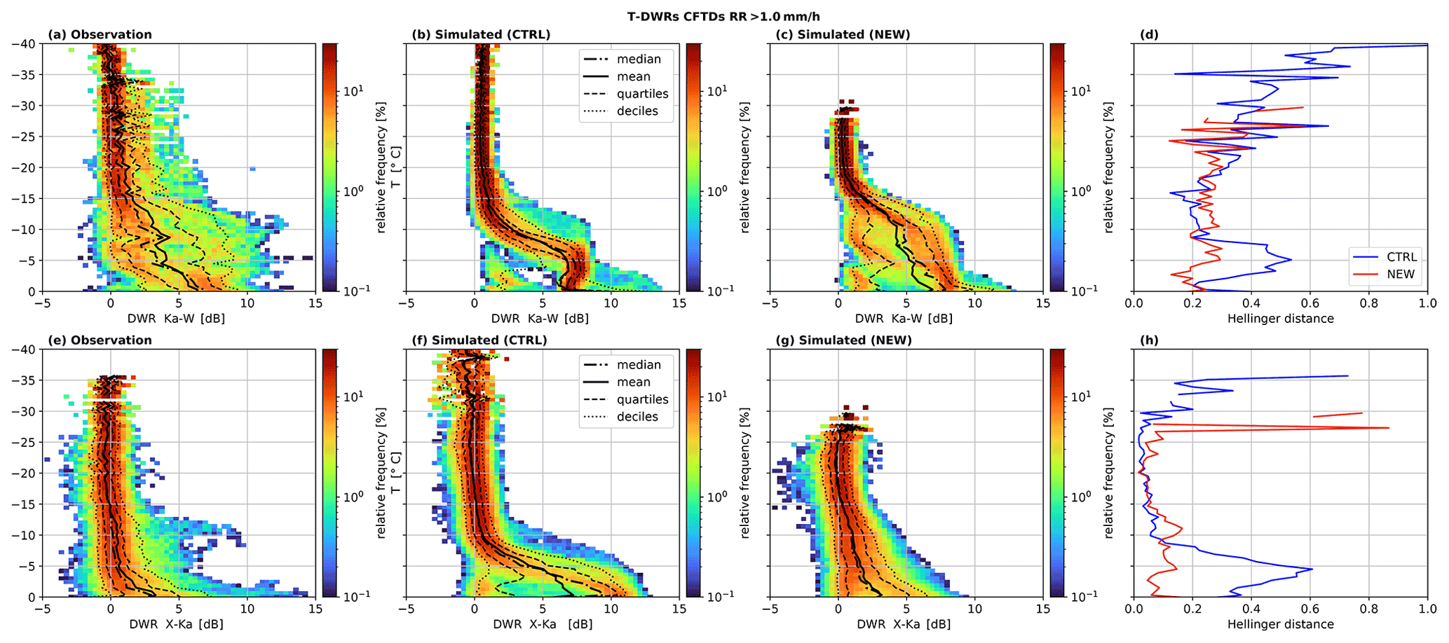
Figure 11Contour frequency by temperature diagrams (CFTDs) for all profiles with RR > 1 mm h−1 of the dual-wavelength ratios between the X and Ka band (DWRX,Ka, top) and between the Ka and W band (DWRX,Ka, bottom) from the default simulation (a, e), the new simulation (colMix2_Akernel; b and f), and measured (c, g). The black lines represent the statistical measures (median, mean, quartiles, and deciles) at different temperatures. Panels (d) and (h) show the Hellinger distance between the simulated and observed distributions for all temperatures.
Besides the overestimation of DWRX,Ka closely above the melting temperature, O20 also highlighted the overestimation of MDV by CTRL. This overestimation is present at all temperatures (compare panels a and b in Fig. 12) and can be attributed to the overestimation of the vt–size relationship of the snow class as reported in Karrer et al. (2020) and the overestimated particle sizes for the higher temperatures. The overestimation of MDV by CTRL is most pronounced for . In this temperature range, CTRL cannot reproduce the asymptotic approach because of the power-law vt–size relationship (Sect. 3.1.3). For example, the median of MDVKa at −5 ∘C is 1 m s−1 in the observations and 1.3 m s−1 in CTRL. In contrast, the new simulations agree better with the observations and H is about half as large as for CTRL. The new scheme setup is more accurate in this temperature range because the Atlas-type vt–size relationship of the Mix2 particles (Fig. 3) correctly considers the asymptotic approach to 1 m s−1 at large sizes. However, MDV is slightly underestimated by NEW for ∘C. Values substantially above 1 m s−1 occur in the observations and the new simulations only closely above the melting temperature, where rain is present. At temperatures below −15 ∘C, both simulations perform similarly, with H ranging from 0.2 to 0.5. While CTRL exhibits a continuous overestimation of MDV, the new simulations lack the observed increase in MDV for ∘C. At these temperatures, the selected PSD width (Sect.3.1.1) and cloud ice particle properties (Sect. 3.1.3) may not be ideal.
The statistical comparison shows that the changes we made to the model could eliminate the most striking biases, namely the overestimation of DWRX,Ka and MDV closely above the melting temperatures. The match of these quantities is important for accurate simulation of precipitation, as exemplified in the case study in Sect. 3.3. Some discrepancies remain, namely the overly strong increase in the DWRs at temperatures between −15 and −10 ∘C and the overestimation (underestimation) of MDV temperatures below −25 ∘C (above −10 ∘C). These discrepancies can be caused by several model errors (inaccurate simulation of, e.g., PSD shape, Estick, degree of riming, variability in cloud ice properties) that cannot be fully deciphered by this observational setup and could benefit from advances in laboratory measurements, observational setup, and representation of cloud ice habits and riming degree in the model.
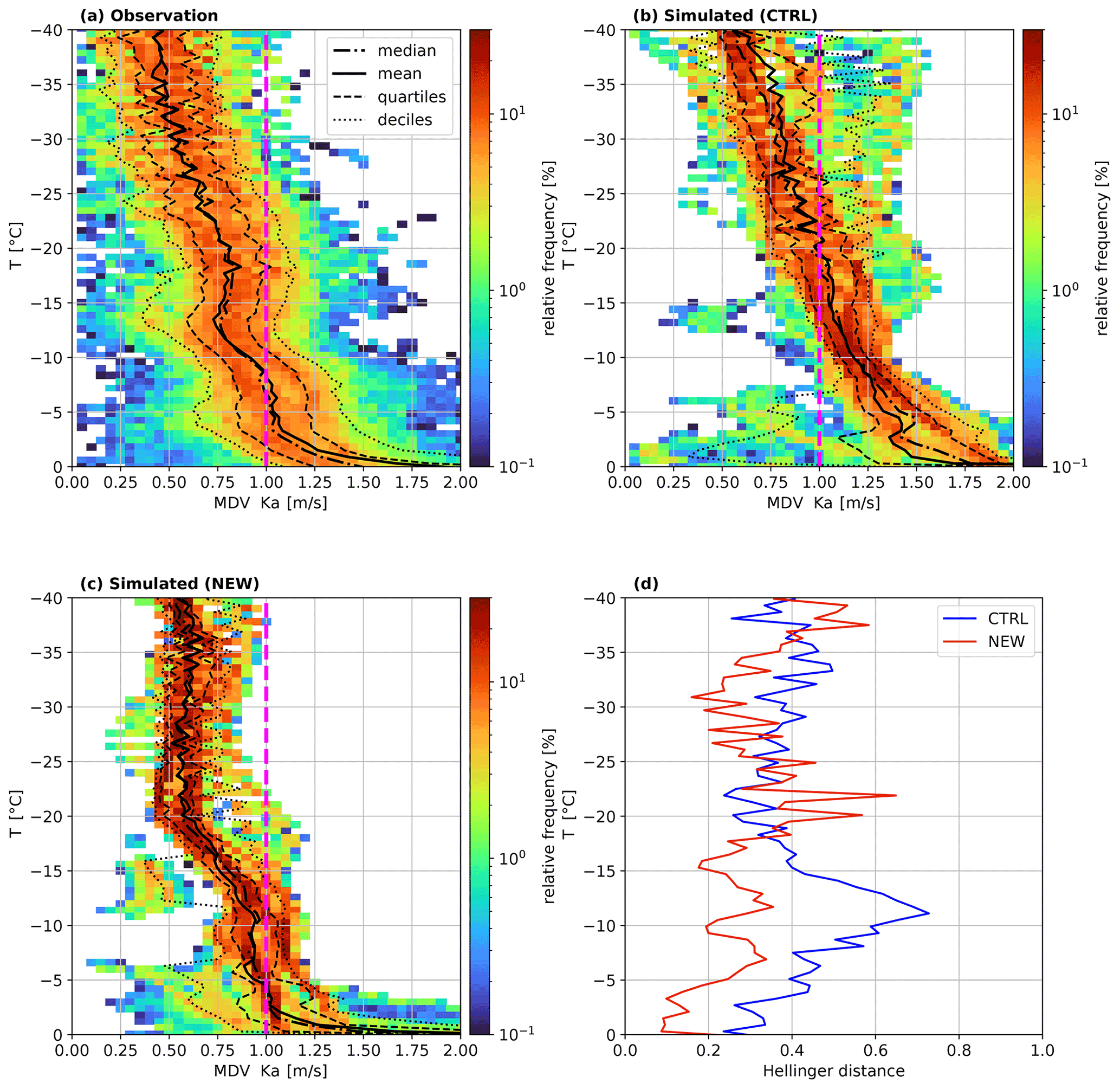
Figure 12Contour frequency by temperature diagrams (CFTDs) of the mean Doppler velocity of the Ka band (MDVKa) from the default simulation (a, e), the new simulation (colMix2_Akernel, b and f), and measured (c, g). The black lines represent the statistical measures (median, mean, quartiles, and deciles) at different temperatures. The histograms on top are calculated including all data and on the bottom only data from profiles for which the precipitation rate RR exceeds 1 mm h−1. A vertical line at 1 m s−1 eases the comparison of the different distributions. Panels (d) and (h) show the Hellinger distance between the simulated and observed distributions for all temperatures.
Aggregation is a key ice microphysical growth process for the formation of precipitating ice particles, which are the precursor of raindrops in cold rain formation. Recent studies using statistics from multi-frequency Doppler radar observations provided observational constraints on how critical radar quantities, such as DWRs or MDV, change with temperature. In this study, we aimed at a deeper analysis of the underlying causes for the observed discrepancies between radar statistics and a state-of-the-art two-moment microphysical scheme, and we improved its simulation of aggregation.
To this end, as a first step, we revisited all relevant components of aggregation as considered in the two-moment scheme to see how well they represent current knowledge of physics. These components are the size distribution width, the temperature dependence of Estick, the particle properties (with a focus on the vt–size relation of aggregates), and the representation of nonspherical particles in the aggregation kernel formulation.
To systematically test the sensitivities of various parameter combinations, we performed 1D simulations with the snowshaft model, which uses simple profiles of thermodynamic variables and a simple initialization of particles at the model top. Moreover, the model only accounts for a subset of all the microphysical processes that occur in real clouds. Nevertheless, by adjusting the model setup we could match the average profiles of radar observables obtained by the 3D simulations of O20, which used the SB06 default scheme setup.
The snowshaft simulations revealed high sensitivity of aggregation to particle properties, the aggregation kernel formulation, and Estick. Surprisingly, the size distribution width had a relatively small effect on the modeled mean mass but a considerable influence on the simulated DWRs. The influence of the cloud ice properties was small in both the model and radar variables.
By comparing the profiles from the snowshaft simulation with the average observed profiles, we were able to select a set of parameters that provided the best agreement with the observations. In this selection process, we mainly varied the less-known components, e.g., the size distribution width, and held other parameters constant that we could better constrain, e.g., the vt–size relationship. The size distribution width proved to be a critical component in linking modeled to observed DWRs and at the same time is difficult to constrain with the given observational setup. Therefore, using a microphysical scheme that explicitly simulates the width of the size distribution (e.g., a three-moment scheme) would provide a more consistent link between the model and observation. However, additional observational constraints from radar (e.g., Doppler spectrum width) and in situ observations should be considered in this case. In particular, we find that the vt–size relationship, which accounts for the asymptotic behavior of vt at large sizes, leads to better agreement with the observations. Moreover, the A-kernel appears to be a better approximation of the aggregation kernel when combined with a constant Ecoll.
We implemented this improved scheme setup in the ICON-LEM and also tested the individual model modifications in a case study. These more realistic ICON-LEM simulations allowed us to derive potential differences in the analysis of sensitivities compared to the snowshaft simulations, possibly caused by effects such as dynamics and advection. Overall, the ICON-LEM simulations yielded similar sensitivities as the snowshaft simulations, but slight differences were apparent with respect to sensitivity to Estick. The differences between simulations with different Estick parameterization were less pronounced in the ICON-LEM simulations. This discrepancy between the simulation frameworks could result from accounting for feedback from microphysics to model humidity in the ICON-LEM simulation.
On the day considered in the case study, relatively dry low-level air resulted in strong sublimation of ice particles. This sublimation feature demonstrated the relevancy of accurately simulating . The SB06 default scheme with its largely overestimated aggregate sizes strongly overestimated the rainfall rate on the ground because the large snowflakes could not sublimate fast enough. In contrast, the more realistic aggregate sizes obtained with the new scheme were able to fit the observations much better.
Finally, the entire period of the campaign dataset (46 d) was simulated again with ICON-LEM using the best-matching parameter combination from the previous tests. This allowed us to directly compare the new statistics with the previous analysis of the default scheme provided in O20. The new aggregation formulation is clearly able to reduce the observed overestimation of MDV. This improvement can be attributed to the new Atlas-type vt–size relationship. The overestimation of the mean particle size at high temperatures revealed in the DWRs was also substantially reduced by the new aggregation parameterization.
Remaining discrepancies are found for DWRs at temperatures of about −12 ∘C and for MDV at low and high temperatures. The overestimated DWRs by the new simulations could result in an overestimated or overly broad size distribution in the model. Inclusion of a higher-frequency radar (Battaglia et al., 2014) may help to infer the particle growth above −12 ∘C. The analysis of Doppler spectra (e.g., similar to Barrett et al., 2019) or observational techniques, e.g., in situ probing of the particle size distribution, would provide additional constraints on the size distribution and ease the interpretation of the MDV and DWR. The mismatch of the MDV at lower temperatures could be caused by an inaccurate size distribution width, as well as Estick or cloud ice properties. Future studies could focus on this temperature region, which is highly relevant for cloud radiative effects. The slight underestimation of MDV at high temperatures could be due to underestimated riming rates, the representation of partially rimed particles, or other effects such as vertical air motion. Further insight could be gained, e.g., from the analysis of the Doppler spectra or comparison with other microphysical schemes with a different representation of the riming process (Morrison and Milbrandt, 2015; Tsai and Chen, 2020).
In addition to the results obtained in this study for aggregation in the SB06 scheme, we think that our approach for how to utilize state-of-the-art radar datasets to improve parameterizations may also serve as a blueprint for future studies focusing on other processes or microphysical schemes. Therefore, we shortly summarize the approach in general terms with the following points.
-
Revisit components of the physical parameterization.
-
Set up single-column simulations which match the average profiles of simulated observables obtained from long-term 3D simulations with the default scheme setup.
-
Systematically test the sensitivities of various parameter combinations in 1D simulations.
-
Select the model configuration that best matches the observations.
-
Implement model modifications in the 3D model and infer possible differences in sensitivities between a 3D simulation and 1D simulations in a case study.
-
Rerun the long-term 3D simulation using the best-matching parameter combination and investigate the improvements by comparing observations with simulations using the default and the new scheme setup.
We summarize the bulk aggregation formulas for all aggregation processes: ice–snow collection, ice self-collection, and snow self-collection. While the formulations using the D-kernel were already given by Seifert et al. (2014), the formulas using the A-kernel were newly derived in this study.
Combining the definition of the moments,
the SCE (Eq. 4) and its simplifications in the SB06 scheme (Sect. 3.1), an equation can be derived that allows for the calculation of all relevant aggregation rates between particles of the classes i and j:
where Mj,n is the nth moment of the hydrometeor class j, f is the particle size distribution for a selected size variable (Dmax, Deq, or m), K is the aggregation kernel, and m is the particle mass.
Seifert et al. (2014) use the variance approach proposed in Seifert and Beheng (2006), which parameterizes the bulk velocity difference by the square root of the second moment of the velocity differences. In this way, the integral is separated into a term containing the geometrical properties (𝒞n,ij) and a part which contains the velocity difference () to enable the analytical integration.
The expressions of 𝒞n,ij and depend on the expression of the PSDm (Sect. 3.1.1), the formulation of the aggregation kernel (Sect. 3.1.2), and the particle properties (Sect. 3.1.3). The SB06 scheme assumes a modified gamma distribution as a function of mass (Eq. 5), which can be easily converted to a gamma distribution as a function of Deq if (Eq. 7). The particle properties are characterized by power-law relations of m (Eq. 12) and Aact (Eq. 15) vs. Dmax and Deq. In the new scheme, vt of cloud ice and snow is parameterized by an Atlas-type relation as a function of Deq (Eq. 11). Coefficients of the relations can be found in Table 2.
A1 D-kernel
Inserting the D-kernel (Eq. 1) into Eq. (A2), the 𝒞n,ij and can be written as
where 𝒩 is the normalization factor given by
Inserting the Dmax−m relation,
and the PSDm (Eq. 5) into 𝒞n,ij (Eq. A4) and solving the integral, we obtain
where and are equal to of Eq. (90) of SB2006 and is equal to of Eq. (91) of SB2006.
Inserting the velocity relation (Eq. 11) and the size distribution using Deq (Eq. 7) into the velocity variance (Eq. A4) and solving the integral, we obtain
with
A2 A-kernel
Inserting the A-kernel (Eq. 9) into Eq. (A2), the velocity variance and the geometric part of the bulk collision rates can be written as
Inserting the A–Deq relation (Eq. 15) and the size distribution as a function of Deq (Eq. 7) into the geometric part (Eq. A13) and solving the integral leads to
with the following.
Inserting the velocity relation (Eq. 11) and the size distribution as a function of Deq (Eq. 7) into the velocity variance (Eq. A14) and solving the integral, we obtain
with
A3 Ice self-collection
A3.1 D-kernel
For ice self-collection the geometry part (Eq. A13) simplifies to
where is equal to of Eq. (90) of SB2006 and is equal to of Eq. (91) of SB2006.
The velocity variance simplifies to
with
A3.2 A-kernel
For ice self-collection 𝒞 (Eq. A13) simplifies to
with the following.
For small sizes, the parametrization of Aact yields values of Ar larger than 1 (e.g., columns smaller than ; Fig. 3d). For small mean sizes, these particles with unphysical Ar can substantially contribute to 𝒞n,ii. Therefore, we limit Aact to Asphere in Eq. (A30). The effect of this limiter can be seen in the kink of the bulk collision rates (Fig. B3c and d).
Inserting the velocity relation (Eq. 11) and the size distribution using Deq (Eq. 7) into the velocity variance (Eq. A14) and solving the integral, we find
with
A4 Snow self-collection
A4.1 D-kernel
For snow self-collection only the first moment is relevant and 𝒞 (Eq. A13) simplifies to
where is equal to of Eq. (90) of SB2006 and is equal to of Eq. (91) of SB2006.
The velocity variance simplifies to
with
A4.2 A-kernel
𝒞 of the A-kernel for snow self-collection simplifies to
with the following.
The area ratios are limited in the same way as for ice self-collection.
The velocity variance simplifies to
with
Table A1Prefactor Φ of the aggregation rates (Eq. A2) for different aggregation processes and the predicted moments of the cloud ice and snow distribution.
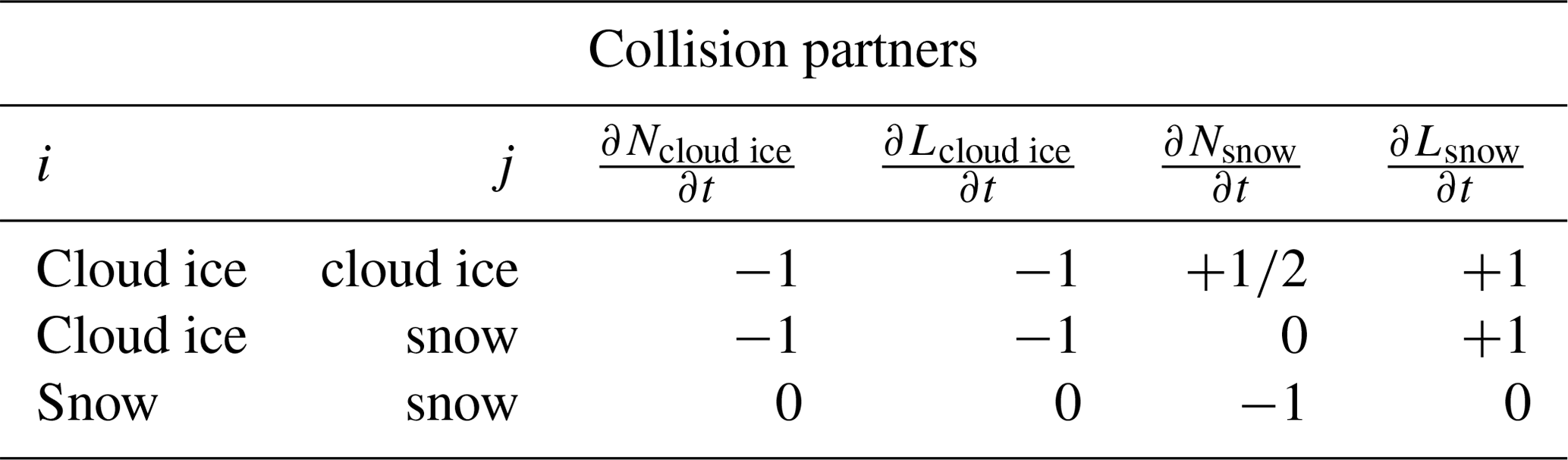
Figure B5 shows the atmospheric variables from O20 simulations and the setup for the snowshaft simulations. Figure B6 shows the atmospheric variables of the case study.
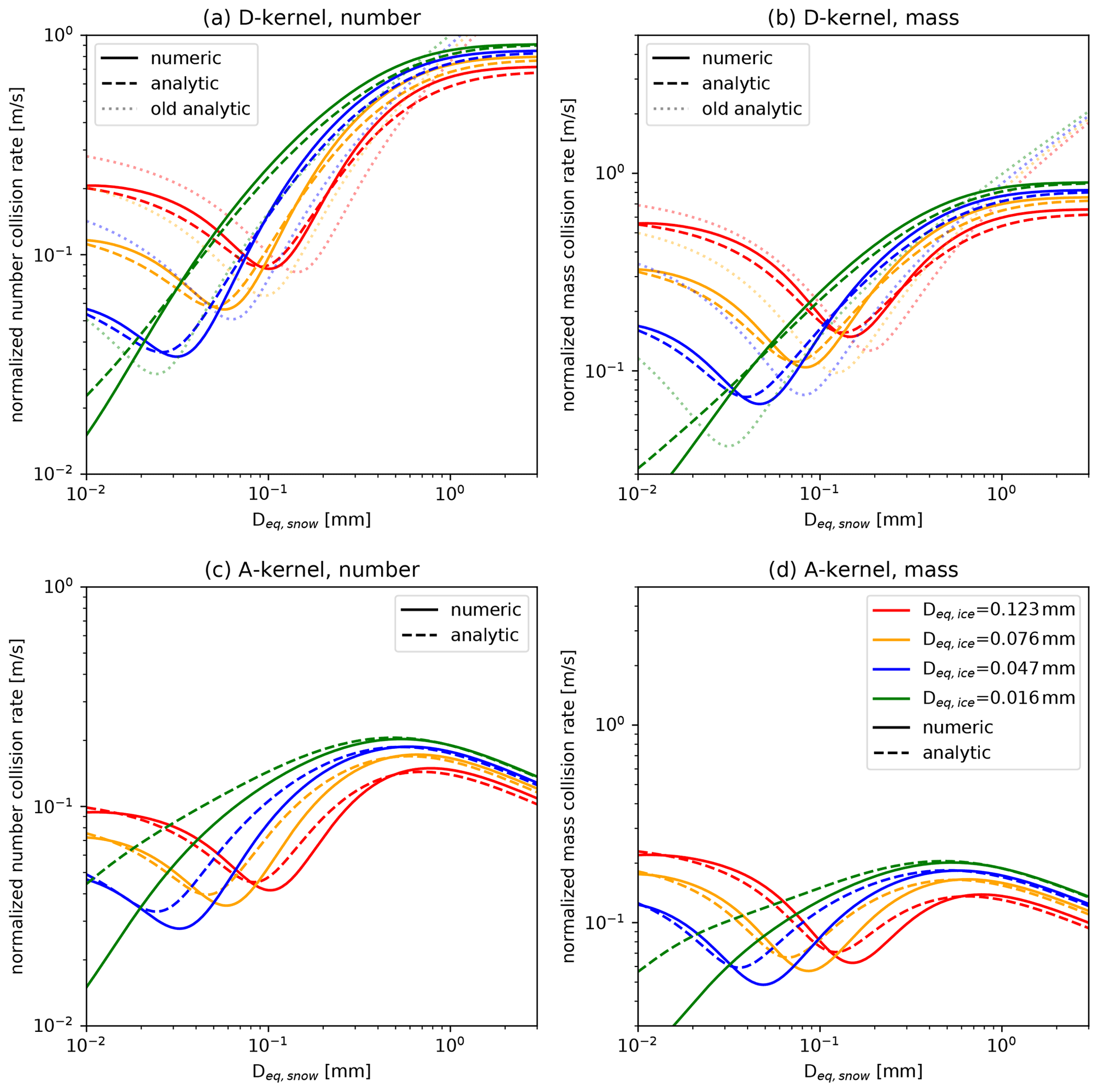
Figure B1Numeric and analytic solution of the bulk collision rates for ice–snow (column and Mix2, respectively) collisions for Atlas-type and power-law velocity size relations. The shape parameter is μeq=2 (Eq. 7), which is equal to μm=0 (Eq. 5) for cloud ice and snow. Left: number density, right: mass density; top: D-kernel; bottom: A-kernel. (a, c) normalized number collision rate, (b, d) normalized mass collision rate, (a, b) D-kernel, (c, d) A-kernel.

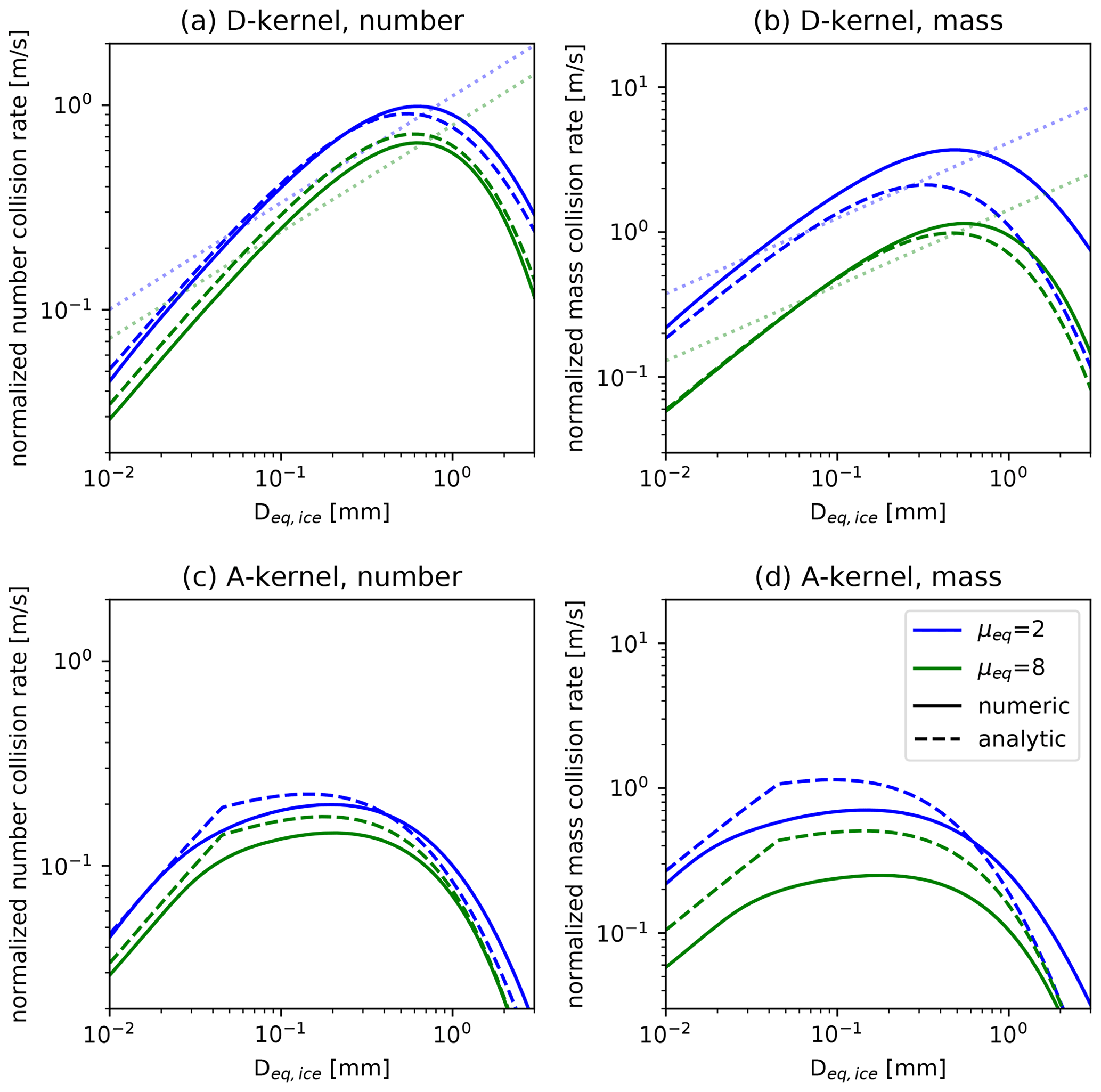
Figure B3Numeric and analytic solution of the bulk collision rates for ice–ice (both column) collisions: (a, c) normalized number collision rate, (b, d) normalized mass collision rate, (a, b) D-kernel, (c, d) A-kernel.
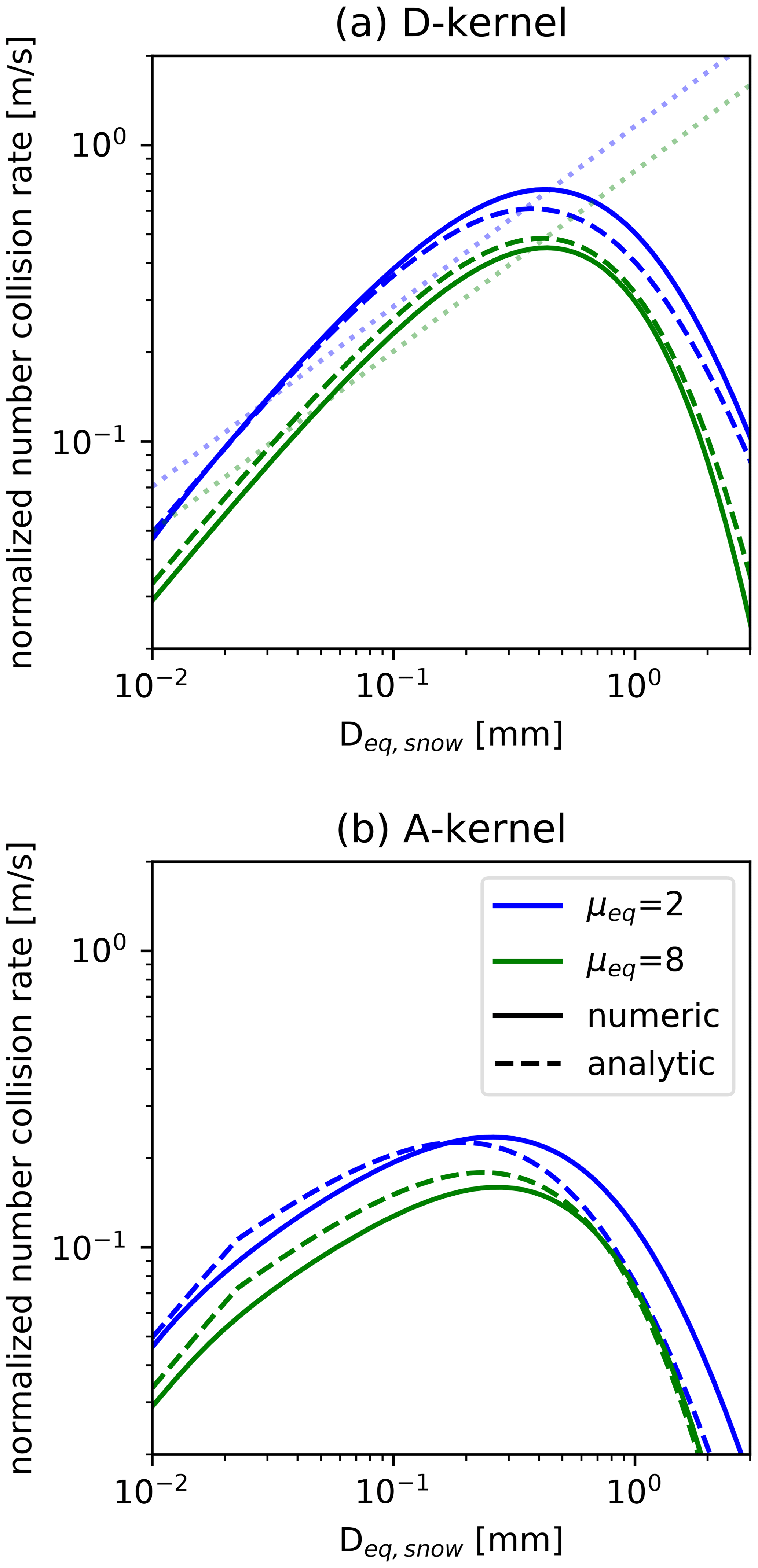
Figure B4Numeric and analytic solution of the bulk collision rates for snow–snow (both Mix2) collisions: (a) D-kernel; (b) A-kernel.

Figure B5Setup of atmospheric variables in the 1D simulations (Sect. 3.2) (black line), which was chosen based on the histograms from the ICON-LEM simulation (the histogram is shown in the background, O20). The histogram is filtered to include only profiles for which the rain rate exceeds 1 mm h−1. (a) Temperature, (b) relative humidity with respect to water, and (c) relative humidity with respect to ice. The height of the melting temperature 0∘C is set to 0 m, and other heights are calculated assuming a temperature gradient of 0.0062 K m−1. Counts in the ICON-LEM simulations from O20 are color-coded.

Figure B6Temperature (a), vertical velocity (b), and relative humidity with respect to water (c) and ice (d) over Jülich in the SB06 default simulation on 3 January 2016. Temperature isolines are shown in each plot.
The source code of the snowshaft model is part of the McSnow model. McSnow and the code to test and optimize the variance approximation of the bulk collision integrals (COLLINT) are hosted on GitLab. The DWD software used in this study (McSnow, COLLINT, etc.) is part of the ICON modeling framework, and access can be granted by AS based on an ICON license agreement. The version of ICON used in this study is available at: https://doi.org/10.5281/zenodo.4740092, Karrer et al., 2021).
The supplement related to this article is available online at: https://doi.org/10.5194/acp-21-17133-2021-supplement.
MK performed and analyzed the snowshaft and ICON-LEM simulation. MK and AS derived the new bulk aggregation formulations. MK and DO performed the forward operation and analyzed the statistics of the multi-month ICON-LEM simulations. SK supervised the project. MK and SK prepared the paper with contributions from all co-authors.
The authors declare that they have no conflicts of interest.
Publisher's note: Copernicus Publications remains neutral with regard to jurisdictional claims in published maps and institutional affiliations.
Contributions by Markus Karrer, Stefan Kneifel, and Davide Ori were funded by the German Research Foundation (DFG) under grant KN 1112/2-1 as part of the Emmy-Noether Group “Optimal combination of Polarimetric and Triple Frequency radar techniques for Improving Microphysical process understanding of cold clouds” (OPTIMIce). AS received funding from the German Science Foundation (DFG) under grant SE 1784/3-1, project ID 408011764 (IMPRINT), as part of the DFG priority program SPP 2115 (PROM) on radar polarimetry. Markus Karrer also acknowledges support by the Graduate School of Geosciences at the University of Cologne. We thank Vera Schemann for support with the ICON-LEM simulations. This work used resources of the Deutsches Klimarechenzentrum (DKRZ) granted by its Scientific Steering Committee (WLA) under project ID bb1086. We also acknowledge the constructive comments of two anonymous reviewers, which helped to improve the paper.
This research has been supported by the Deutsche Forschungsgemeinschaft (grant no. KN 1112/2-1; grant no. SE 1784/3-1, project ID 408011764 (IMPRINT)) as part of the DFG priority program SPP 2115 (PROM).
This paper was edited by Franziska Glassmeier and reviewed by two anonymous referees.
Andrić, J., Kumjian, M. R., Zrnić, D. S., Straka, J. M., and Melnikov, V. M.: Polarimetric signatures above the melting layer in winter storms: An observational and modeling study, J. Appl. Meteorol. Clim., 52, 682–700, https://doi.org/10.1175/JAMC-D-12-028.1, 2013. a
Barrett, A. I., Westbrook, C. D., Nicol, J. C., and Stein, T. H. M.: Rapid ice aggregation process revealed through triple-wavelength Doppler spectrum radar analysis, Atmos. Chem. Phys., 19, 5753–5769, https://doi.org/10.5194/acp-19-5753-2019, 2019. a, b, c, d, e, f, g
Barthazy, E. and Schefold, R.: Fall velocity of snowflakes of different riming degree and crystal types, Atmos. Res., 82, 391–398, https://doi.org/10.1016/j.atmosres.2005.12.009, 2006. a
Battaglia, A., Westbrook, C. D., Kneifel, S., Kollias, P., Humpage, N., Löhnert, U., Tyynelä, J., and Petty, G. W.: G band atmospheric radars: new frontiers in cloud physics, Atmos. Meas. Tech., 7, 1527–1546, https://doi.org/10.5194/amt-7-1527-2014, 2014. a
Battaglia, A., Tanelli, S., Tridon, F., Kneifel, S., Leinonen, J., and Kollias, P.: Triple-Frequency Radar Retrievals, Adv. Glob. Change Res., 67, 211–229, https://doi.org/10.1007/978-3-030-24568-9_13, 2020. a
Böhm, J. P.: A general hydrodynamic theory for mixed-phase microphysics. Part I: drag and fall speed of hydrometeors, Atmos. Res., 27, 253–274, https://doi.org/10.1016/0169-8095(92)90035-9, 1992. a
Connolly, P. J., Emersic, C., and Field, P. R.: A laboratory investigation into the aggregation efficiency of small ice crystals, Atmos. Chem. Phys., 12, 2055–2076, https://doi.org/10.5194/acp-12-2055-2012, 2012. a, b, c
Cotton, W. R., Stephens, M. A., Nehrkorn, T., and Tripoli, G. J.: The Colorado State University three-dimensional cloud/mesoscale model 1982 – Part II: an ice phase parameterization, Journal de Recherches Atmospheriques, 16, 295–320, 1982. a, b
Dias Neto, J., Kneifel, S., Ori, D., Trömel, S., Handwerker, J., Bohn, B., Hermes, N., Mühlbauer, K., Lenefer, M., and Simmer, C.: The TRIple-frequency and Polarimetric radar Experiment for improving process observations of winter precipitation, Earth Syst. Sci. Data, 11, 845–863, https://doi.org/10.5194/essd-11-845-2019, 2019. a
Dipankar, A., Stevens, B., Heinze, R., Moseley, C., Zängl, G., Giorgetta, M., and Brdar, S.: Large eddy simulation using the general circulation model ICON, J. Adv. Model. Earth Sys., 7, 963–986, https://doi.org/10.1002/2015MS000431, 2015. a
Dunnavan, E. L.: How snow aggregate ellipsoid shape and orientation variability affects fall speed and self-aggregation rates, J. Atmos. Sci., 78, 51–73, https://doi.org/10.1175/JAS-D-20-0128.1, 2021. a
Field, P. R.: Bimodal ice spectra in frontal clouds, Q. J. Roy. Meteor. Soc., 126, 379–392, https://doi.org/10.1002/qj.49712656302, 2000. a
Field, P. R., Hogan, R. J., Brown, P. R., Illingworth, A. J., Choularton, T. W., and Cotton, R. J.: Parametrization of ice-particle size distributions for mid-latitude stratiform cloud, Q. J. Roy. Meteor. Soc., 131, 1997–2017, https://doi.org/10.1256/qj.04.134, 2005. a
Gillespie, D. T.: Three Models for the Coalescence Growth of Cloud Drops., J. Atmos. Sci., 32, 600–607, https://doi.org/10.1175/1520-0469(1975)032<0600:TMFTCG>2.0.CO;2, 1975. a
Hashino, T. and Tripoli, G. J.: The Spectral Ice Habit Prediction System (SHIPS). Part IV: Box model simulations of the habit-dependent aggregation process, J. Atmos. Sci., 68, 1142–1161, https://doi.org/10.1175/2011JAS3667.1, 2011. a
Heinze, R., Dipankar, A., Henken, C. C., Moseley, C., Sourdeval, O., Trömel, S., Xie, X., Adamidis, P., Ament, F., Baars, H., Barthlott, C., Behrendt, A., Blahak, U., Bley, S., Brdar, S., Brueck, M., Crewell, S., Deneke, H., Di Girolamo, P., Evaristo, R., Fischer, J., Frank, C., Friederichs, P., Göcke, T., Gorges, K., Hande, L., Hanke, M., Hansen, A., Hege, H. C., Hoose, C., Jahns, T., Kalthoff, N., Klocke, D., Kneifel, S., Knippertz, P., Kuhn, A., van Laar, T., Macke, A., Maurer, V., Mayer, B., Meyer, C. I., Muppa, S. K., Neggers, R. A., Orlandi, E., Pantillon, F., Pospichal, B., Röber, N., Scheck, L., Seifert, A., Seifert, P., Senf, F., Siligam, P., Simmer, C., Steinke, S., Stevens, B., Wapler, K., Weniger, M., Wulfmeyer, V., Zängl, G., Zhang, D., and Quaas, J.: Large-eddy simulations over Germany using ICON: a comprehensive evaluation, Q. J. Roy. Meteor. Soc., 143, 69–100, https://doi.org/10.1002/qj.2947, 2017. a
Heymsfield, A. J.: Properties of Tropical and Midlatitude Ice Cloud Particle Ensembles, Part II: Applications for Mesoscale and Climate Models in: Journal of the Atmospheric Sciences Volume 60 Issue 21 (2003), J. Atmos. Sci., 60, 2592–2611, 2003. a, b
Heymsfield, A. J. and Westbrook, C. D.: Advances in the estimation of ice particle fall speeds using laboratory and field measurements, J. Atmos. Sci., 67, 2469–2482, https://doi.org/10.1175/2010JAS3379.1, 2010. a
Heymsfield, A. J., Schmitt, C., Chen, C. C. J., Bansemer, A., Gettelman, A., Field, P. R., and Liu, C.: Contributions of the Liquid and Ice Phases to Global Surface Precipitation: Observations and Global Climate Modeling, J. Atmos. Sci., 77, 2629–2648, https://doi.org/10.1175/JAS-D-19-0352.1, 2020. a
Hobbs, P. V., Chang, S., and Locatelli, J. D.: The dimensions and aggregation of ice crystals in natural clouds, J. Geophys. Res., 79, 2199–2206, https://doi.org/10.1029/jc079i015p02199, 1974. a
Hogan, R. J. and Westbrook, C. D.: Equation for the microwave backscatter cross section of aggregate snowflakes using the self-similar Rayleigh-Gans approximation, J. Atmos. Sci., 71, 3292–3301, https://doi.org/10.1175/JAS-D-13-0347.1, 2014. a
Hogan, R. J., Illingworth, A. J., and Sauvageot, H.: Measuring crystal size in cirrus using 35- and 94-GHz radars, J. Atmos. Ocean. Tech., 17, 27–37, https://doi.org/10.1175/1520-0426(2000)017<0027:MCSICU>2.0.CO;2, 2000. a
Hogan, R. J., Honeyager, R., Tyynelä, J., and Kneifel, S.: Calculating the millimetre-wave scattering phase function of snowflakes using the self-similar Rayleigh–Gans Approximation, Q. J. Roy. Meteor. Soc., 143, 834–844, https://doi.org/10.1002/qj.2968, 2017. a
Hosler, C. L. and Hallgren, R. E.: The aggregation of small ice crystals, Discussions of the Faraday Society, 30, 200–207, https://doi.org/10.1039/DF9603000200, 1960. a
Illingworth, A. J., Hogan, R. J., O'Connor, E. J., Bouniol, D., Brooks, M. E., Delanoë, J., Donovan, D. P., Eastment, J. D., Gaussiat, N., Goddard, J. W., Haeffelin, M., Klein Baltinik, H., Krasnov, O. A., Pelon, J., Piriou, J. M., Protat, A., Russchenberg, H. W., Seifert, A., Tompkins, A. M., van Zadelhoff, G. J., Vinit, F., Willen, U., Wilson, D. R., and Wrench, C. L.: Cloudnet: Continuous evaluation of cloud profiles in seven operational models using ground-based observations, B. Am. Meteorol. Soc., 88, 883–898, https://doi.org/10.1175/BAMS-88-6-883, 2007. a
Kajikawa, M. and Heymsfield, A. J.: Aggregation of ice crystals in cirrus, https://doi.org/10.1175/1520-0469(1989)046<3108:AOICIC>2.0.CO;2, 1989. a, b
Kalesse, H., Szyrmer, W., Kneifel, S., Kollias, P., and Luke, E.: Fingerprints of a riming event on cloud radar Doppler spectra: observations and modeling, Atmos. Chem. Phys., 16, 2997–3012, https://doi.org/10.5194/acp-16-2997-2016, 2016. a, b
Kanji, Z. A., Ladino, L. A., Wex, H., Boose, Y., Burkert-Kohn, M., Cziczo, D. J., and Krämer, M.: Overview of Ice Nucleating Particles, Meteorol. Monogr., 58, 1–33, https://doi.org/10.1175/AMSMONOGRAPHS-D-16-0006.1, 2017. a
Karrer, M., Seifert, A., Siewert, C., Ori, D., von Lerber, A., and Kneifel, S.: Ice Particle Properties Inferred From Aggregation Modelling, J. Adv. Model. Earth Sys., 12, e2020MS002066, https://doi.org/10.1029/2020MS002066, 2020. a, b, c
Karrer, M.: ICON-LEM version used for the publication “Improving the Representation of Aggregation in a Two-moment Microphysical Scheme with Statistics of Multi-frequency Doppler Radar Observations”, Zenodo [code], https://doi.org/10.5281/zenodo.4740092, 2021. a
Keith, W. D. and Saunders, C. P.: The collection efficiency of a cylindrical target for ice crystals, Atmos. Res., 23, 83–95, https://doi.org/10.1016/0169-8095(89)90059-8, 1989. a
Kennedy, P. C. and Rutledge, S. A.: S-band dual-polarization radar observations of winter storms, J. Appl. Meteorol. Clim., 50, 844–858, https://doi.org/10.1175/2010JAMC2558.1, 2011. a
Khain, A. P., Beheng, K. D., Heymsfield, A., Korolev, A., Krichak, S. O., Levin, Z., Pinsky, M., Phillips, V., Prabhakaran, T., Teller, A., Van Den Heever, S. C., and Yano, J. I.: Representation of microphysical processes in cloud-resolving models: Spectral (bin) microphysics versus bulk parameterization, Rev. Geophys., 53, 247–322, https://doi.org/10.1002/2014RG000468, 2015. a
Kienast-Sjögren, E., Spichtinger, P., and Gierens, K.: Formulation and test of an ice aggregation scheme for two-moment bulk microphysics schemes, Atmos. Chem. Phys., 13, 9021–9037, https://doi.org/10.5194/acp-13-9021-2013, 2013. a
Kneifel, S. and Moisseev, D. N.: Long-term statistics of riming in nonconvective clouds derived from ground-based doppler cloud radar observations, J. Atmos. Sci., 77, 3495–3508, https://doi.org/10.1175/JAS-D-20-0007.1, 2020. a
Kneifel, S., Von Lerber, A., Tiira, J., Moisseev, D. N., Kollias, P., and Leinonen, J.: Observed relations between snowfall microphysics and triple-frequency radar measurements, J. Geophys. Res., 120, 6034–6055, https://doi.org/10.1002/2015JD023156, 2015. a, b, c
Kneifel, S., Leinonen, J., Tyynelä, J., Ori, D., and Battaglia, A.: Scattering of Hydrometeors, in: Advances in Global Change Research, Springer, 67, 249–276, https://doi.org/10.1007/978-3-030-24568-9_15, 2020. a, b
Korolev, A. and Leisner, T.: Review of experimental studies of secondary ice production, Atmos. Chem. Phys., 20, 11767–11797, https://doi.org/10.5194/acp-20-11767-2020, 2020. a, b
Kumjian, M. R. and Ryzhkov, A. V.: The impact of evaporation on polarimetric characteristics of rain: Theoretical model and practical implications, J. Appl. Meteorol. Clim., 49, 1247–1267, https://doi.org/10.1175/2010JAMC2243.1, 2010. a
Lamb, D. and Verlinde, J.: Physics and chemistry of clouds, Cambridge University Press, https://doi.org/10.1017/CBO9780511976377, 2011. a, b, c
Liao, L., Meneghini, R., Iguchi, T., and Detwiler, A.: Use of dual-wavelength radar for snow parameter estimates, J. Atmos. Ocean. Tech., 22, 1494–1506, https://doi.org/10.1175/JTECH1808.1, 2005. a
Lin, Y. L., Farley, R. D., and Orville, H. D.: Bulk parameterization of the snow field in a cloud model., J. Clim. Appl. Meteorol., 22, 1065–1092, https://doi.org/10.1175/1520-0450(1983)022<1065:BPOTSF>2.0.CO;2, 1983. a, b
Lohmann, U., Lüönd, F., and Mahrt, F.: An introduction to clouds: From the microscale to climate, Cambridge University Press, https://doi.org/10.1017/CBO9781139087513, 2016. a
Löhnert, U., Schween, J. H., Acquistapace, C., Ebell, K., Maahn, M., Barrera-Verdejo, M., Hirsikko, A., Bohn, B., Knaps, A., O'Connor, E., Simmer, C., Wahner, A., and Crewell, S.: JOYCE: Jülich Observatory for Cloud Evolution, B. Am. Meteorol. Soc., 96, 1157–1174, https://doi.org/10.1175/BAMS-D-14-00105.1, 2015. a
Marke, T., Crewell, S., Schemann, V., Schween, J. H., and Tuononen, M.: Long-term observations and high-resolution modeling of midlatitude nocturnal boundary layer processes connected to low-level jets, J. Appl. Meteorol. Clim., 57, 1155–1170, https://doi.org/10.1175/JAMC-D-17-0341.1, 2018. a
Mason, S. L., Hogan, R. J., Westbrook, C. D., Kneifel, S., Moisseev, D., and von Terzi, L.: The importance of particle size distribution and internal structure for triple-frequency radar retrievals of the morphology of snow, Atmos. Meas. Tech., 12, 4993–5018, https://doi.org/10.5194/amt-12-4993-2019, 2019. a
Mason, S. L., Chiu, C. J., Hogan, R. J., Moisseev, D. N., and Kneifel, S.: Retrievals of Riming and Snow Density From Vertically Pointing Doppler Radars, J. Geophys. Res.-Atmos., 123, 13807–13834, https://doi.org/10.1029/2018JD028603, 2018. a, b
Matrosov, S. Y.: A dual-wavelength radar method to measure snowfall rate, J. Appl. Meteorol., 37, 1510–1521, https://doi.org/10.1175/1520-0450(1998)037<1510:ADWRMT>2.0.CO;2, 1998. a
Mcfarquhar, G. M., Hsieh, T. L., Freer, M., Mascio, J., and Jewett, B. F.: The characterization of ice hydrometeor gamma size distributions as volumes in N0-λ-μ phase space: Implications for microphysical process modeling, J. Atmos. Sci., 72, 892–909, https://doi.org/10.1175/JAS-D-14-0011.1, 2015. a
Mech, M., Maahn, M., Kneifel, S., Ori, D., Orlandi, E., Kollias, P., Schemann, V., and Crewell, S.: PAMTRA 1.0: the Passive and Active Microwave radiative TRAnsfer tool for simulating radiometer and radar measurements of the cloudy atmosphere, Geosci. Model Dev., 13, 4229–4251, https://doi.org/10.5194/gmd-13-4229-2020, 2020. a
Milbrandt, J. A. and Morrison, H.: Parameterization of cloud microphysics based on the prediction of bulk ice particle properties, Part III: Introduction of multiple free categories, J. Atmos. Sci., 73, 975–995, https://doi.org/10.1175/JAS-D-15-0204.1, 2016. a
Mitchell, D. L.: Evolution of snow-size spectra in cyclonic storms. Part I: snow growth by vapor deposition and aggregation, J. Atmos. Sci., 45, 3431–3451, https://doi.org/10.1175/1520-0469(1988)045<3431:EOSSSI>2.0.CO;2, 1988. a, b
Mitchell, D. L.: Use of mass- and area-dimensional power laws for determining precipitation particle terminal velocities, J. Atmos. Sci., 53, 1710–1723, https://doi.org/10.1175/1520-0469(1996)053<1710:UOMAAD>2.0.CO;2, 1996. a
Mitchell, D. L. and Heymsfield, A. J.: Refinements in the treatment of ice particle terminal velocities, highlighting aggregates, J. Atmos. Sci., 62, 1637–1644, https://doi.org/10.1175/JAS3413.1, 2005. a
Moisseev, D. N., Lautaportti, S., Tyynela, J., and Lim, S.: Dual-polarization radar signatures in snowstorms: Role of snowflake aggregation, J. Geophys. Res., 120, 12644–12665, https://doi.org/10.1002/2015JD023884, 2015. a
Morrison, H. and Milbrandt, J. A.: Parameterization of cloud microphysics based on the prediction of bulk ice particle properties. Part I: Scheme description and idealized tests, J. Atmos. Sci., 72, 287–311, https://doi.org/10.1175/JAS-D-14-0065.1, 2015. a, b, c
Morrison, H., van Lier-Walqui, M., Fridlind, A. M., Grabowski, W. W., Harrington, J. Y., Hoose, C., Korolev, A., Kumjian, M. R., Milbrandt, J. A., Pawlowska, H., Posselt, D. J., Prat, O. P., Reimel, K. J., Shima, S. I., van Diedenhoven, B., and Xue, L.: Confronting the Challenge of Modeling Cloud and Precipitation Microphysics, J. Adv. Model. Earth Sys., 12, 2019MS001689, https://doi.org/10.1029/2019MS001689, 2020. a, b
Mosimann, L.: An improved method for determining the degree of snow crystal riming by vertical Doppler radar, Atmos. Res., 37, 305–323, https://doi.org/10.1016/0169-8095(94)00050-N, 1995. a, b
Ori, D., Schemann, V., Karrer, M., Dias Neto, J., von Terzi, L., Seifert, A., and Kneifel, S.: Evaluation of ice particle growth in ICON using statistics of multi-frequency Doppler cloud radar observations, Q. J. Roy. Meteor. Soc., 146, 3830–3849, https://doi.org/10.1002/qj.3875, 2020. a
Ori, D., von Terzi, L., Karrer, M., and Kneifel, S.: snowScatt 1.0: consistent model of microphysical and scattering properties of rimed and unrimed snowflakes based on the self-similar Rayleigh–Gans approximation, Geosci. Model Dev., 14, 1511–1531, https://doi.org/10.5194/gmd-14-1511-2021, 2021. a, b, c, d
Paukert, M., Fan, J., Rasch, P. J., Morrison, H., Milbrandt, J. A., Shpund, J., and Khain, A.: Three-Moment Representation of Rain in a Bulk Microphysics Model, J. Adv. Model. Earth Sys., 11, 257–277, https://doi.org/10.1029/2018MS001512, 2019. a
Pfitzenmaier, L., Unal, C. M. H., Dufournet, Y., and Russchenberg, H. W. J.: Observing ice particle growth along fall streaks in mixed-phase clouds using spectral polarimetric radar data, Atmos. Chem. Phys., 18, 7843–7862, https://doi.org/10.5194/acp-18-7843-2018, 2018. a, b
Phillips, V. T., Formenton, M., Bansemer, A., Kudzotsa, I., and Lienert, B.: A parameterization of sticking efficiency for collisions of snow and graupel with ice crystals: Theory and comparison with observations, J. Atmos. Sci., 72, 4885–4902, https://doi.org/10.1175/JAS-D-14-0096.1, 2015. a
Pruppacher, H. and Klett, J.: Hydrodynamics of Single Cloud and Precipitation Particles, PhD. thesis, https://doi.org/10.1007/978-0-306-48100-0_10, 2010. a
Pruppacher, H. R., Klett, J. D., and Wang, P. K.: Microphysics of Clouds and Precipitation, Aerosol Sci. Technol., 28, 381–382, https://doi.org/10.1080/02786829808965531, 1998. a, b
Reitter, S., Fröhlich, K., Seifert, A., Crewell, S., and Mech, M.: Evaluation of ice and snow content in the global numerical weather prediction model GME with CloudSat, Geosci. Model Dev., 4, 579–589, https://doi.org/10.5194/gmd-4-579-2011, 2011. a
Schemann, V. and Ebell, K.: Simulation of mixed-phase clouds with the ICON large-eddy model in the complex Arctic environment around Ny-Ålesund, Atmos. Chem. Phys., 20, 475–485, https://doi.org/10.5194/acp-20-475-2020, 2020. a
Schemann, V., Ebell, K., Pospichal, B., Neggers, R., Moseley, C., and Stevens, B.: Linking Large-Eddy Simulations to Local Cloud Observations, J. Adv. Model. Earth Sys., 12, e2020MS002209, https://doi.org/10.1029/2020MS002209, 2020. a
Schmidt, G. A., Bader, D., Donner, L. J., Elsaesser, G. S., Golaz, J.-C., Hannay, C., Molod, A., Neale, R. B., and Saha, S.: Practice and philosophy of climate model tuning across six US modeling centers, Geosci. Model Dev., 10, 3207–3223, https://doi.org/10.5194/gmd-10-3207-2017, 2017. a
Schrom, R. S. and Kumjian, M. R.: Connecting microphysical processes in colorado winter storms with vertical profiles of radar observations, J. Appl. Meteorol. Clim., 55, 1771–1787, https://doi.org/10.1175/JAMC-D-15-0338.1, 2016. a
Seifert, A.: On the parameterization of evaporation of raindrops as simulated by a one-dimensional rainshaft model, J. Atmos. Sci., 65, 3608–3619, https://doi.org/10.1175/2008JAS2586.1, 2008. a, b, c
Seifert, A. and Beheng, K. D.: A two-moment cloud microphysics parameterization for mixed-phase clouds, Part 1: Model description, Meteorol. Atmos. Phys., 92, 45–66, https://doi.org/10.1007/s00703-005-0112-4, 2006. a, b, c, d, e, f
Seifert, A., Blahak, U., and Buhr, R.: On the analytic approximation of bulk collision rates of non-spherical hydrometeors, Geosci. Model Dev., 7, 463–478, https://doi.org/10.5194/gmd-7-463-2014, 2014. a, b, c, d, e, f
Slater, B. and Michaelides, A.: Surface premelting of water ice, Nature Reviews Chemistry, 3, 172–188, https://doi.org/10.1038/s41570-019-0080-8, 2019. a, b, c
Szyrmer, W. and Zawadzki, I.: Snow Studies. Part IV: Ensemble Retrieval of Snow Microphysics from Dual-Wavelength Vertically Pointing Radars, J. Atmos. Sci., 71, 1158–1170, 2014. a
Tridon, F., Battaglia, A., and Kneifel, S.: Estimating total attenuation using Rayleigh targets at cloud top: applications in multilayer and mixed-phase clouds observed by ground-based multifrequency radars, Atmos. Meas. Tech., 13, 5065–5085, https://doi.org/10.5194/amt-13-5065-2020, 2020. a
Tsai, T. C. and Chen, J. P.: Multimoment ice bulk microphysics scheme with consideration for particle shape and apparent density. Part I: Methodology and idealized simulation, J. Atmos. Sci., 77, 1821–1850, https://doi.org/10.1175/JAS-D-19-0125.1, 2020. a
Verlinde, J., Flatau, P. J., and Cotton, W. R.: Analytical solutions to the collection growth equation: comparison with approximate methods and application to cloud microphysics parameterization schemes, J. Atmos. Sci., 47, 2871–2880, https://doi.org/10.1175/1520-0469(1990)047<2871:ASTTCG>2.0.CO;2, 1990. a
Wang, P. K.: Physics and dynamics of clouds and precipitation, Vol. 9781107005, Cambridge University Press, https://doi.org/10.1017/CBO9780511794285, 2010. a
Wisner, C., Orville, H. D., and Myers, C.: A Numerical Model of a Hail-Bearing Cloud, J. Atmos. Sci., 29, 1160–1181, 1972. a, b, c, d
Zängl, G., Reinert, D., Rípodas, P., and Baldauf, M.: The ICON (ICOsahedral Non-hydrostatic) modelling framework of DWD and MPI-M: Description of the non-hydrostatic dynamical core, Q. J. Roy. Meteor. Soc., 141, 563–579, https://doi.org/10.1002/qj.2378, 2015. a, b
- Abstract
- Introduction
- Methods
- Results and discussion
- Conclusions
- Appendix A: Bulk aggregation rates
- Appendix B: Atmospheric setup for 1D simulation and atmospheric fields of the case study predicted by ICON-LEM
- Code availability
- Author contributions
- Competing interests
- Disclaimer
- Acknowledgements
- Financial support
- Review statement
- References
- Supplement