A climatology of trade-wind cumulus cold pools and their link to mesoscale cloud organization

We present a climatology of trade cumulus cold pools and their associated changes in surface weather, vertical velocity and cloudiness based on more than 10 years of in situ and remote sensing data from the Barbados Cloud Observatory. Cold pools are identified by abrupt drops in surface temperature, and the mesoscale organization pattern is classified by a neural network algorithm based on Geostationary Operational Environmental Satellite 16 (GOES-16) Advanced Baseline Imager (ABI) infrared images. We find cold pools to be ubiquitous in the winter trades – they are present about 7.8 % of the time and occur on 73 % of days. Cold pools with stronger temperature drops (ΔT) are associated with deeper clouds, stronger precipitation, downdrafts and humidity drops, stronger wind gusts and updrafts at the onset of their front, and larger cloud cover compared to weaker cold pools, which agrees well with the conceptual picture of cold pools. The rain duration in the front is the best predictor of ΔT and explains 36 % of its variability.

The mesoscale organization pattern has a strong influence on the occurrence frequency of cold pools. Fish has the largest cold-pool fraction (12.8 % of the time), followed by Flowers and Gravel (9.9 % and 7.2 %) and lastly Sugar (1.6 %). Fish cold pools are also significantly stronger and longer-lasting compared to the other patterns, while Gravel cold pools are associated with significantly stronger updrafts and deeper cloud-top height maxima. The diel cycle of the occurrence frequency of Gravel, Flowers, and Fish can explain a large fraction of the diel cycle in the cold-pool occurrence as well as the pronounced extension of the diel cycle of shallow convection into the early afternoon by cold pools. Overall, we find cold-pool periods to be ∼ 90 % cloudier relative to the average winter trades. Also, the wake of cold pools is characterized by above-average cloudiness, suggesting that mesoscale arcs enclosing broad clear-sky areas are an exception. A better understanding of how cold pools interact with and shape their environment could therefore be valuable to understand cloud cover variability in the trades.

1 Introduction

Satellite images in the trades usually show very beautiful and diverse cloud structures over the dark blue ocean. Recurrent features in these images are mesoscale arcs of cumuli that encircle either clear-sky areas or extensive stratiform cloud decks. The mesoscale arcs result from spreading cold pools that have favourable conditions at their gust front for triggering new convection. Convective cold pools are generated by the evaporation of precipitation into unsaturated downdrafts, spreading out at the surface as a density current. Cold pools are not only important for the triggering of new and often deeper convection (Schlemmer and Hohenegger, 2014; Feng et al., 2015; Rowe and Houze, 2015), but might also play a role in regulating cloud cover in the trades – a regime responsible for much of the uncertainty in climate sensitivity (Bony and Dufresne, 2005; Vial et al., 2013). Here we use ground-based in situ and remote sensing data from the Barbados Cloud Observatory (BCO) to study the climatology of trade-wind cumulus cold pools and to investigate its link to the pattern of mesoscale cloud organization.

Many studies addressing oceanic cold pools have focused on deep convection (Zuidema et al., 2017). In the trades, detailed case studies for 2 weeks of the Rain in Cumulus over the Ocean (RICO) campaign have advanced our understanding of cold pools from shallow convection (Zuidema et al., 2012). They showed that the deepest clouds and strongest radar signals occurred in the moistest tercile of water vapour paths and that precipitation-driven downdrafts can introduce additional gradients in the thermodynamic structure. More recently, analyses of data from the Elucidating the Role of Clouds-Circulation Coupling in Climate (EUREC⁴A) field campaign (Bony et al., 2017; Stevens et al., 2021), which took place in January and February 2020 upstream Barbados, revealed that cold pools are frequent in the winter trades and can be well detected from soundings due to their very shallow mixed layers (Touzè-Peiffer et al., 2021). What is missing is a long-term climatology of trade cumulus cold pools along with a description of the changes in cloud properties and sub-cloud layer dynamics associated with the cold-pool passages. Such a climatology is particularly pertinent given the need for a reference dataset for comparison against increasingly available high-resolution simulations (Stevens et al., 2019; Rochetin et al., 2021).

Renewed interest in trade cumulus cold pools is also motivated by recent advances in characterizing patterns of mesoscale cloud organization. Stevens et al. (2020) classified 900 satellite images in the North Atlantic trades and identified four prominent patterns of mesoscale cloud organization – Sugar, Gravel, Flowers, and Fish. The horizontal structure of the latter three patterns is intrinsically linked to the occurrence of mesoscale arcs and hence cold pools. The four patterns differ not only in their horizontal structure, but also in cloud cover, cloud depth, and precipitation (Bony et al., 2020; Schulz et al., 2021; Vial et al., 2021). These differences likely also manifest in different cold-pool characteristics. Furthermore, cold pools might play different roles in creating and maintaining these patterns. For the Fish pattern with its very large-scale fish-bone structures that are tightly linked to extratropical dry intrusions (Aemisegger et al., 2021; Schulz et al., 2021), cold pools are likely to give the cloudy part its skeletal structure, while the overall system is forced by the large-scale dynamics into its linear alignment. Observations of drizzling stratocumulus often show cold pools being dragged along with a larger system without initiating its mesoscale organization (Wilbanks et al., 2015). Contrastingly, for the Gravel pattern, the large-scale influence may be less important and also more homogeneous. Thus, cold pools likely play an important role in creating and maintaining this pattern, similar to the strong influence of rain (and indirectly also cold pools) on the transition from closed- to open-cell stratocumulus (Xue et al., 2008; Wang and Feingold, 2009; Glassmeier and Feingold, 2017). Before we can understand the different roles that cold pools play in these patterns, we need to understand whether and how cold-pool characteristics differ among them.

This paper presents the first long-term climatology of trade-wind cumulus cold pools and addresses the following research questions.

1. How frequent are cold pools in the trade cumulus regime, and with what changes in the surface meteorology, cloudiness, and vertical velocity are they associated?

2. How do cold-pool characteristics covary with the pattern of mesoscale organization?

We use more than 10 years of surface meteorology and ground-based remote sensing data from 2011 to 2021 collected at the BCO (Stevens et al., 2016). Clouds, their precipitation, and therefore likely also cold pools at the BCO were shown to be representative across the trades (Medeiros and Nuijens, 2016). Cold pools are identified by abrupt drops in surface temperature, and the pattern of mesoscale organization is classified by a neural network algorithm based on infrared satellite images (Schulz et al., 2021). To focus on trade cumulus cold pools, we limit most of our analysis to the winter regime from December to April, as in summer the intertropical convergence zone is often close to Barbados and convection is much deeper (Brueck et al., 2015).

Section 2.1 presents the data sources and explains the cold-pool detection algorithm and the selection criteria. In Sect. 3, we present the cold-pool climatology and analyse the temporal structure of cold-pool passages and the associated changes in meteorology and cloudiness. Section 4 discusses differences between the cold-pool properties of the different mesoscale organization patterns. Conclusions are presented in Sect. 5.

2 Data and methods

2.1 BCO data

We use in situ and ground-based remote sensing data from the BCO (Stevens et al., 2016), which has been operated by the Max Planck Institute for Meteorology together with the Caribbean Institute for Meteorology and Hydrology since April 2010. The BCO is located atop a 17 m cliff on an eastward promontory of Barbados called Deebles Point (13.16^∘ N, 59.43^∘ W) and samples nearly undisturbed Atlantic trade-wind conditions. We have used surface meteorology and micro-rain radar (MRR) data since January 2011, cloud radar data since January 2012, and Doppler lidar data from March 2016 until March 2021. All data are aggregated into 1 min averages. The instruments used and meteorological variables derived are explained in the following. More details about the BCO and its instrumentation can be found in Nuijens et al. (2014) and Stevens et al. (2016).

2.1.1 Surface meteorology

A Vaisala WXT520 sensor mounted on a 5 m mast measures temperature, relative humidity, barometric pressure, wind speed, and wind direction. We discard temperature measurements exceeding 35 ^∘C and pressure measurements lower than 980 hPa, as they are outside the expected range of variability at the BCO.

2.1.2 MRR

The MRR is a vertically pointing frequency-modulated continuous-wave radar operating at 24 GHz (K band). The MRR data have a temporal resolution of 1 min and a range gate of 30 m up to a height of 3 km. Rain rates lower than 0.03  mm h⁻¹ are below the noise level and set to zero. We derive the mean rain rate (RR) and the rain intensity (R_int, i.e. the instantaneous rain rate during periods of rain) for a specified period from data at 325 m above ground (the lowest level with reliable data). The MRR is also used to compute the rain frequency (R_freq), which is set to 1 when a RR>0.05 mm h⁻¹ is measured in at least five range gates in the lowest 3 km (following Nuijens et al., 2014). A few instances with unrealistically large RR exceeding 200 mm h⁻¹ are set to NA (not applicable).

2.1.3 Cloud radar

Vertical profiles of hydrometeors (including both cloud and rain droplets) at 10 s temporal and 30 m vertical resolution are derived from two 35.5 GHz (Ka-band) Doppler cloud radars. Radar returns with an equivalent radar reflectivity lower than −50 dBZ are removed to eliminate signal from sea salt aerosol (Klingebiel et al., 2019). To identify connected 2D cloud objects, a cloud segmentation algorithm is applied (Konow, 2020). Radar reflectivity is converted to a binary mask and morphological closing is applied to remove noise from measurement interruptions. The resulting mask is used to identify cloud objects using connected component analysis with 8-connectivity. A minimum cloud size of 4 pixels is applied, and everything smaller than 4 pixels is discarded as clutter. To focus on clouds connected to the trade-wind layer, only cloud objects with a lowest cloud-base height (CBH_ID) smaller than 4 km are considered in the analysis.

From the remaining clouds, we derive 1 min averaged time series of the hydrometeor fraction (HF), cloud-base height (CBH), cloud-top height (CTH), and projected cloud cover (CC). Following Nuijens et al. (2014), CC is further split up into contributions from cloud segments with different CBH, which represent cloudiness near the lifting-condensation level (CC_lcl; 300 m < CBH ≤ 1 km) and cloudiness aloft such as stratiform layers or edges of deeper cumuli (CC_aloft; 1 km < CBH ≤ 4 km). We also introduce a third category of precipitating cloud segments if CBH ≤ 300 m (CC_prcp, the same threshold as in Klingebiel et al., 2021). A given 1 min HF profile can only count to one of the three categories, such that e.g. a 2 km-deep cloud with CBH < 300 m will only be counted in the CC_prcp category. Note that the above classification into the different CBH categories does not consider the cloud objects, and subsequent HF profiles are classified independently. A similar analysis accounting for the cloud objects by classifying CC contributions of different cloud objects by their CBH_ID is shown in Appendix A.

2.1.4 Doppler lidar

The vertical velocity in the sub-cloud layer is measured by two Halo Photonics Streamline Pro Doppler wind lidar systems (Päschke et al., 2015) at 30 m vertical resolution. The Doppler lidars measure vertical velocities of up to ±20 m s⁻¹ with a 1500 nm laser at altitudes from about 50 m to 1 km, depending on the atmospheric conditions and the aerosol loading. The precision is < 20 cm s⁻¹ for a signal-to-noise ratio (SNR) of −17 dB. Measurements with a SNR smaller than −18.3 dB are discarded. Data from the first system that was operated in vertically pointing mode with a temporal resolution of 1.3 s are used from March 2016 to October 2019. A second system has been operated in horizontally scanning mode since February 2019 and has a temporal resolution of 3 s, with two out of seven profiles measured in vertically pointing mode. Vertical data from this second lidar are used from November 2019 to March 2021.

We derive 1 min time series of both the average vertical velocity in the sub-cloud layer (SCL) as the mean over 15 range gates from 75 to 495 m (w_SCL) and the vertical velocity near the sub-cloud layer top at 450 m as the mean over the four range gates from 405 to 495 m (w₄₅₀). Doppler lidar vertical velocities are commonly considered reliable also in rainy periods (see e.g. Zhu et al., 2021). We did not encounter problems with the Doppler lidar retrievals in rainy periods, and Figs. 2 and 3h will show that the negative vertical velocities associated with downdrafts are generally well captured.

2.2 Machine learning classification of mesoscale cloud organization patterns

The pattern of mesoscale cloud organization at the BCO for the period January 2018 to March 2021 is classified by a neural network algorithm applied to infrared satellite images from the Geostationary Operational Environmental Satellite 16 (GOES-16). We use brightness temperature retrievals every 30 min from the 10.35 µm channel at a spatial resolution of 2 km from the Advanced Baseline Imager (ABI) Level-1b data product (GOES-R Calibration Working Group and GOES-R Series Program, 2017), over a large domain including Barbados (45–66^∘ W, 9.3–23.3^∘ N).

The neural network based on the RetinaNet algorithm (Lin et al., 2017) was initially trained on and applied to visible images in Rasp et al. (2020) and later retrained and applied to infrared images by Schulz et al. (2021). The use of infrared images also allows study of the diurnal cycle of the mesoscale organization (Vial et al., 2021). The classifications of the neural network are rectangles of various sizes that belong to either the Sugar, Gravel, Flowers, or Fish pattern. We select every classified rectangle that overlaps with the BCO location. Periods without a classification are labelled as “No”. The BCO data at 1 min resolution are considered contemporaneous with the nearest 30 min neural network classification. If a given pattern is present for more than 75 % of the duration of a cold pool, the cold pool is categorized by this pattern.

At any given time, multiple rectangles of different sizes of the same and different patterns can occur. Multiple rectangles of the same pattern are combined and counted only once, while multiple rectangles of different patterns are counted separately. This leads to locations in the images, and hence data in the meteorological time series, being classified e.g. as both Gravel and Flowers. Excluding situations with multiple patterns only marginally influences the results but reduces the sample size considerably (as previously noted in Vial et al., 2021). Ambiguities in the classification can be physical – for example due to regime transitions or similarities between patterns – or related to ambiguities introduced to the neural network by disagreement in the human classifications. The occurrence of multiple patterns can be reduced if a stricter threshold is used for the agreement score representing the confidence of the neural network prediction (here set to 0.4 as in Schulz et al., 2021; Vial et al., 2021), but this again reduces the sample size.

2.3 Cold-pool detection algorithm

We detect cold pools by identifying abrupt drops in the BCO surface temperature time series following Vogel (2017). We first filter the 1 min averaged temperature time series with an 11 min running average. We then classify all filtered 1 min temperature drops $\mathit{\delta }T=T_{\mathrm{fil}}\left(t\right)-T_{\mathrm{fil}}(t-\mathrm{1})<-\mathrm{0.05}$ K (per minute) as a cold-pool candidate (see Fig. 1 for an illustration). For every candidate cold pool, we detect the time of the cold-pool front onset (t_max), the time of the minimum temperature (t_min), and the end of the cold pool (t_end) as follows.

1. t_max: the onset of the cold-pool front t_max is defined as the last instance of δT>0 K within 20 min before the initial abrupt temperature drop with $\mathit{\delta }T<-\mathrm{0.05}$ K. If the temperature is falling continuously in this period, t_max is chosen as the time of the maximum temperature (that is, 20 min before the abrupt temperature drop). We refer to the smoothed temperature at t_max as T_max.

2. t_min: the time of the minimum filtered temperature T_min marks the end of the cold-pool front and is identified as the minimum of contiguous temperature minima. Subsequent candidate cold pools with $\mathit{\delta }T<-\mathrm{0.05}$ K occurring within 20 min of the previous minimum are combined if the temperature does not rise by more than 0.5 K above the previous minimum in between.

3. t_end: the end of a cold pool is defined either as the minimum of (a) the time when the filtered temperature first exceeds its minimum by $\mathrm{\Delta }T/e$, where $\mathrm{\Delta }T=T_{\max }-T_{\min }$ is the total filtered temperature drop in the cold pool and e is Euler's number, or (b) the onset of the next cold pool. If using condition (a) or (b) leads to any temperature between t_min and t_end being smaller than T_min−0.15 K, then t_end is defined as (c) the time when the filtered temperature first decreases again after increasing for some time following t_min. Cold pools with t_end defined by (a) are referred to as recovered.

The period between t_max and t_min is referred to as the cold-pool front and the period between t_min and t_end as the cold-pool wake.

Figure 1 Illustration of the cold-pool detection algorithm. (a) 11 min filtered T_fil (thick line) and 1 min raw surface temperature (thin line), and (bottom) filtered temperature difference δT along with the threshold of −0.05 K used (dashed). The detected cold-pool fronts and wakes are indicated in dark grey (t_max to t_min) and light grey (t_min to t_end), with the corresponding ΔT indicated at the top. The dark red lines in (a) show the analysis periods used for computing the diagnostics (see Sect. 2.5).

Our cold-pool detection algorithm is similar to the one used by de Szoeke et al. (2017) but with the important modification that we only identify cold pools for situations with abrupt temperature drops exceeding our threshold of $\mathit{\delta }T<-\mathrm{0.05}$ K. With our algorithm we thus filter out both turbulent fluctuations and advective or diurnal patterns of temperature variability. The threshold of $\mathit{\delta }T<-\mathrm{0.05}$ K is subjectively chosen based on visual impression and represents distinct variations in temperature. For an 11 min averaging window, a δT of −0.05 K corresponds to about 2 % of the data. Figure 2 shows example cold pools for all patterns and illustrates the algorithm. In the next subsection we briefly discuss the strengths and weaknesses of the algorithm based on these examples.

2.4 Example cases

Time series of example cold-pool days along with corresponding satellite images are shown for every pattern in Fig. 2 and shed some light on the differences in the cold-pool characteristics of the four patterns. The two Sugar cold pools stem from isolated precipitating deeper cumuli. The satellite image captures the deeper cloud over the BCO at the time of the first cold pool and also indicates some organization of the cumuli in lines upstream the BCO, while the canonical Sugar fields of shallow cumuli pass further north. The textbook-like Gravel example day is characterized by many short and often weak cold pools quickly following each other, interspersed by stronger cold pools. The stronger cold pools are associated with the presence of strongly precipitating deeper clouds (note that the radar did not work prior to 12:00 LT). The many cold pools present on this day clearly imprint their signature on the satellite image in the form of mesoscale arcs.

The cold pools on the Flowers day are associated with the large cloud system whose stratiform layer reaches the BCO at 10:00 LT. Three cold pools are directly associated with the large system, with the first one starting at 11:00 LT, showing a very strong ΔT of −3.85 K. The large system has rain rates up to 3.6 mm h⁻¹ and is preceded by a weaker cold pool at 09:30 LT associated with the very thin mesoscale arc visible in the satellite image. This first weak cold pool goes along with a strong increase in humidity of 1.3 g kg⁻¹. The Fish day features a 6 h-long cold pool associated with steady and intense rain (maximum RR of 11.6 mm h⁻¹), continued strong downdrafts, and very high humidity throughout its entire duration. The temperature fully recovers within about 20 min of the cold-pool end, and 3 h later two subsequent pronounced cold pools follow that are again characterized by continued precipitation and downdrafts. The satellite image shows the fish-bone-like cloud band typically associated with the Fish pattern, which is strongly connected to trailing cold fronts of extratropical origins (Aemisegger et al., 2021; Schulz et al., 2021). The more front-like character of the Fish cold pools with steady showers and downdrafts is clearly evident. While most of the cooling is expected to stem from the evaporating precipitation, we cannot rule out a small cooling contribution related to a larger-scale temperature contrast between the south and north of the Fish cloud band (see also Schulz et al., 2021).

The example cases highlight how well the detection algorithm works in these diverse situations. Abrupt strong temperature drops are reliably detected, successive fronts sensibly combined into one single cold pool, and even the 6 h-long cold pool with frontal character on the Fish day is correctly identified.

The examples also indicate some challenges of the cold-pool identification. Although they look like cold pools, some temperature drops on the Gravel and Sugar days are not identified as cold pools because they are either not abrupt enough ($\mathit{\delta }T\ge -\mathrm{0.05}$ K) or not strong enough ($\mathrm{\Delta }T\ge -\mathrm{0.4}$ K). The difficulty in defining the end of the cold-pool wake is illustrated in the Fish case: the cold pool starting shortly before 16:00 LT lasts until well after 18:00 LT, but the temperature drop near 17:00 LT causes a premature end of the cold pool. A temperature drop of this magnitude could also be caused by the diel cycle in temperature. The cold-pool end definition could be improved by an additional rain or downdraft requirement to more robustly distinguish between cold-pool activity and other processes. Because most analyses and diagnostics computed in this study focus entirely on the cold-pool front (see next section), not fully representing the wake of rare long-lasting cold pools is a minor issue that could only influence the overall cold-pool fraction and the duration statistics.

As mentioned in Sect. 2.2, the organization pattern definition is somewhat ambiguous. Also among the example days shown in Fig. 2, multiple cloud patterns pertain to some cold pools. For the Flowers case, the 2 h at the beginning and end of the period shown are also classified, respectively, as Gravel and Fish. In the Sugar case, only the period between 09:00 and 16:00 LT is exclusively classified as Sugar, while the periods before and after are also partly classified as Gravel. Most surprisingly, the textbook Gravel day is also entirely classified as Flowers, and also setting a stricter agreement score of 0.5 leaves half of the day co-classified as Flowers. This indicates that distinguishing Gravel from Flowers can be particularly challenging (as also shown in Vial et al., 2021). The Fish day is very confidently classified and no other pattern is detected for the entire day.

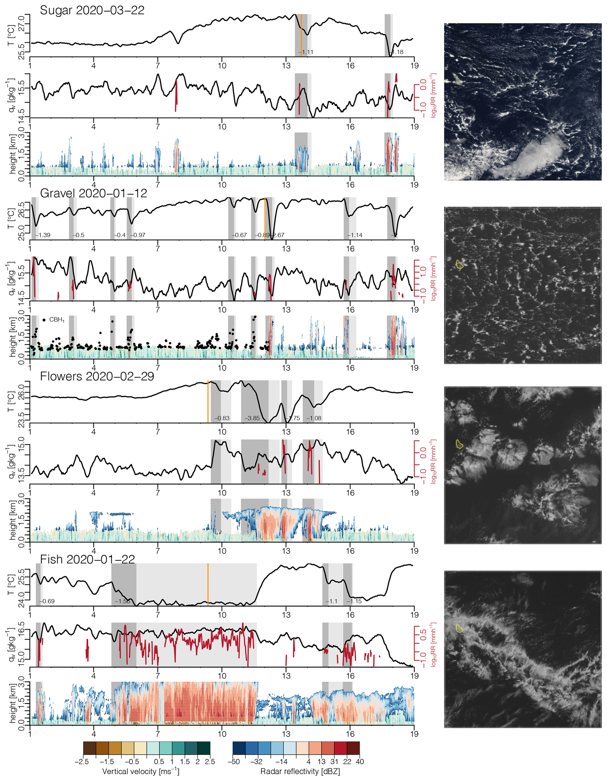
Figure 2 BCO time series and satellite images for 18 h of 4 cold-pool days representative of the four patterns. Shown are time series of filtered surface temperature and specific humidity, MRR rain rate, and time–height plots of Doppler lidar vertical velocity and radar reflectivity. On the Gravel day the radar did not work prior to 12:00 LT, and the first ceilometer cloud base (CBH₁) is shown instead. The x axis shows local time and the detected cold-pool fronts and wakes are indicated in grey and light grey, with ΔT indicated at the bottom. Visible satellite images from 10–15^∘ N, 60–55^∘ W are from MODIS Aqua (Sugar day) and GOES-16 ABI (other days), with the respective recording times indicated by the orange lines in the temperature panels. The BCO is located near the easternmost tip of Barbados (outlined in yellow).

2.5 Selection criteria and diagnostics

For the subsequent analyses, we apply a number of selection criteria to make the comparison of cold pools more robust. That is, we only consider cold pools with $\mathrm{\Delta }T<-\mathrm{0.4}$ K and less than two missing values in the filtered temperature time series during the entire cold-pool duration (set all with 9234 cold pools). For the analyses of the cold-pool properties we further apply a criterion of no non-recovered cold pool in the hour prior to the cold-pool onset (set noprev with 8772 cold pools), which selects cold pools moving into an initially undisturbed atmosphere that is not modified by previous convection. Except for Appendix B, we also focus on the dry winter regime from December to April (set noprevWI with 3889 cold pools), which is characterized by steady easterlies, subsiding large-scale motion in the free troposphere and the predominance of shallow trade-wind convection (Brueck et al., 2015).

All these selection criteria reduce the cold-pool sample size considerably. They represent a trade-off between ensuring a robust and unbiased sample to address our research questions while not being unnecessarily strict and removing too many cold pools. The selection criteria are thus somewhat subjective and differ among studies. For example, Chandra et al. (2018) used the criterion of no rain in the hour prior to the cold-pool onset to select cold pools unmodified by previous convection, whereas we achieve the same goal with the criterion of no non-recovered cold pool in the prior hour, which excludes less cold pools in our case (i.e. about 2500 additional cold pools would be discarded with the criterion of Chandra et al., 2018). Instead of focusing on the winter regime, we could have also set a criterion based on the cloud-top height to focus on trade cumulus cold pools. However, as this would restrict the analysis to periods when the radar is running and – as we are relying on single-site measurements – the parent convection might not move over the BCO in its entirety, we would likely exclude too many cold pools with a CTH criterion without even being sure that periods of deep convection are really excluded. Despite the rather strict criteria applied here, the long time series leads to a much larger number of cold pools analysed than in previous studies.

Another potential sampling issue regarding the single-site measurements is that it is not clear at which stage of its life cycle we sample the cold pool and where we sample it with respect to its centre. Assuming azimuthally symmetric wind variations around the cold-pool centre, which in case of little wind shear is a good approximation (Touzè-Peiffer et al., 2021), the change in wind direction from the mean direction prior to the cold-pool onset could give a hint as to the location relative to the cold-pool centre. Due to our large sample size, a potential random bias is likely to be small. The influence of wind shear on the propagation direction and characteristics of cold pools is an interesting topic for a future study.

If not mentioned differently, diagnostics for each cold pool are computed either as the minimum difference (ΔX_min) or maximum difference (ΔX_max) of a variable X across the cold-pool duration, e.g. $\mathrm{\Delta }{X}_{\max }=\max \left(X\right((t_{\max }+\mathrm{1}):t_{\mathrm{end}})-X(t_{\max })$). If the cold-pool wake lasts longer than 20 min, the diagnostics are computed only until 20 min after t_min (instead of until t_end) to prevent problems in case of a poorly defined cold-pool end. Similarly, X_mean or X_max are the mean or maximum of variable X over the same analysis period (indicated in dark red in Fig. 1). For the Doppler lidar vertical velocities, we diagnose w_maxSCL (w_max450) as the maximum w_SCL (w₄₅₀) in the first half of the front (including the last 10 min before t_max) and w_minSCL as the minimum w_SCL in the second half of the front (including the first 10 min after t_min). Unless otherwise stated, the surface meteorology diagnostics are computed from the 11 min filtered time series.

Along with most diagnostics and composites, we show the standard error (SE), which measures how well the median or mean of a given sample can be estimated. The SE of the median is computed as $\mathrm{IQR}/\sqrt{n}$, where IQR represents the inter-quartile range and n the sample size, and the SE of the mean as $\mathit{\sigma }/\sqrt{n}$, where σ is the standard deviation. As not all instruments were running all the time, some diagnostics are only available for a subset of the cold pools, and the sample size is adjusted accordingly when computing the SE.

3 Cold-pool climatology

In this section we present the climatology of trade cumulus cold pools detected at the BCO for the winter seasons of the years 2011–2021. The first subsection presents general statistics, followed by a discussion of the composite temporal structure of the cold pools in Sect. 3.2. The diel cycle of cold-pool statistics is shown in Sect. 3.3. While our focus lies on the winter regime, Appendix B also briefly discusses the seasonal cycle of the cold-pool statistics.

3.1 General statistics

In total we detect 3889 cold pools that meet the criteria of $\mathrm{\Delta }T<-\mathrm{0.4}$ K and less than two missing values in T_fil in the winter seasons considered. We find that cold pools are very frequent at the BCO, and on 73 % of days at least one cold pool is detected. The BCO is on average affected by cold pools during 7.8 % of the day (i.e. 112 min) and by a cold-pool front during 4.4 % of the day. The median daily cold-pool fractions are about one-third smaller than the means mentioned, indicating that there are some days with a very large cold-pool fraction. The mean daily cold-pool fraction of 8.6 % for January and February 2011–2021 is also very close to the 7 % found by Touzè-Peiffer et al. (2021) during the EUREC⁴A campaign in January and February 2020, despite their very different method defining cold pools in atmospheric soundings based on a mixed-layer depth criterion.

Table 1 Table showing median ± IQR of various cold-pool properties for the noprevWI set of cold pools as well as the 25 % strongest ($\mathrm{\Delta }T<-\mathrm{1.39}$ K) and weakest ($\mathrm{\Delta }T>-\mathrm{0.61}$ K) cold pools of this set. The computation of the diagnostics is explained in Sect. 2.5.

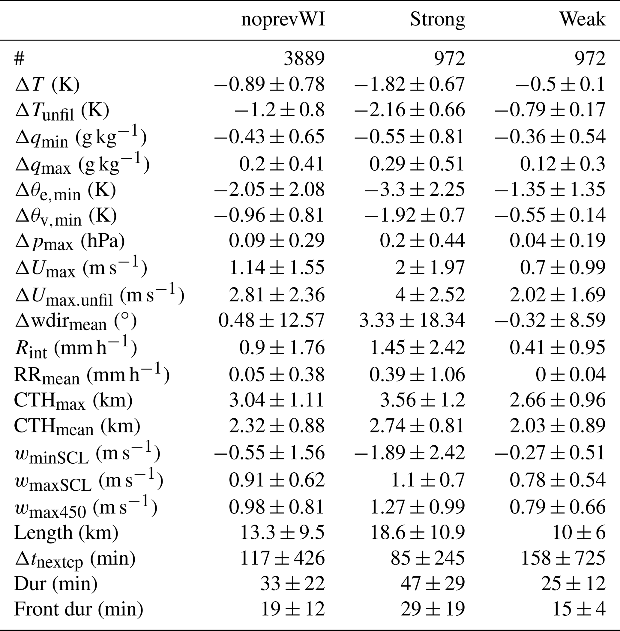
Table 1 presents statistics of the most important cold-pool properties for the set of winter cold pools with no non-recovered cold pool in the prior hour (noprevWI). It shows that 50 % of the cold pools have a temperature drop exceeding 0.9 K across the front (the unfiltered temperature drop is 0.3 K stronger), a Δq_max exceeding 0.2 g kg⁻¹ and a Δq_min below −0.43 g kg⁻¹, decreases in θ_e and θ_v exceeding −2.1 K and −0.96 K, respectively, a Δp_max exceeding 9 Pa, and a ΔU_max larger than 1.14 m s⁻¹ (with the unfiltered anomaly being more than twice as large). The median rain intensity measured by the MRR is 0.9 mm h⁻¹. Furthermore, 50 % of the cold pools are associated with a maximum cloud-top height exceeding 3 km and w_maxSCL and w_minSCL of 0.9 m s⁻¹ and −0.55 m s⁻¹ near the onset and end of the front, respectively.

The average cold-pool duration is 33 min, of which a bit more than half of the time pertains to the front. Multiplying the duration by the surface wind speed yields a median cold-pool length larger than 13.3 km. This median cold-pool duration and length may seem small compared to satellite imagery, in which mesoscale cold-pool arcs can easily span 100 km. Also, the largest 2 % of cold pools are hardly larger than 40 km. The smaller cold-pool sizes found here are likely due to the algorithm sampling mostly the edge of the cold pools and due to the challenges of defining the cold-pool end purely based on the surface temperature time series (see discussion in Sect. 2.4).

The IQR shows that all these medians are associated with substantial variability, especially for the humidity and rain variables. However, focusing on the winter regime generally reduces the IQR of the diagnostics compared to all seasons (not shown), suggesting that this criterion indeed results in a more homogeneous cold-pool sample representative of the trade cumulus regime.

Table 1 also compares the median ± IQR of the 25 % strongest and weakest cold pools in terms of ΔT. The strongest cold pools last longer, follow each other more quickly (lower Δt_nextcp), and are associated with deeper clouds, more rain, stronger downdrafts, humidity drops and wind gusts, and larger positive vertical velocities at the beginning of the front compared to weaker cold pools. This agrees well with the conceptual picture of deeper clouds producing more rain and having a larger potential for rain evaporation, which drives stronger downdrafts that bring down more dry air from further aloft and which induces a stronger cooling and a stronger gust front that is associated with stronger rising motion at its leading edge. Similar but slightly smaller differences between stronger and weaker cold pools are found when comparing cold pools associated with the 25 % strongest versus weakest downdrafts or the 25 % deepest versus shallowest CTH_max (not shown).

The rain duration in the front is the diagnostic that explains most variability in ΔT (R²=0.364). Rain duration is well correlated (R=0.47) with the front duration, which itself explains a comparable amount of variability in ΔT (R²=0.357). That the accumulated rain amount in the front explains less variability in ΔT (R²=0.21) than the rain duration indicates that the rain intensity is of secondary importance. Another important predictor of ΔT is the downdraft strength w_minSCL (R²=0.23), which together with the front duration explains 50 % of the variability in ΔT for the noprevWI set. The CTH usually scales with the precipitation amount for trade cumuli (Byers and Hall, 1955; Kubar et al., 2009; Nuijens et al., 2009), and CTH_max also explains some variability in ΔT (R²=0.10). That the rain duration, the downdraft strength, and the maximum CTH also distinguish the cold-pool properties well indicates that the parent convection triggering the cold pool is sampled well by the single-point measurements.

3.2 Composite temporal structure

Figure 3 shows the composite mean temporal structure of the perturbations associated with the cold-pool passages. To facilitate the comparison of different cold pools, we use a normalized time coordinate within the cold-pool front with values after t_max and before t_min mapped onto 20 points (the median front duration), similar to previous studies (Young et al., 1995; de Szoeke et al., 2017; Zuidema et al., 2017).

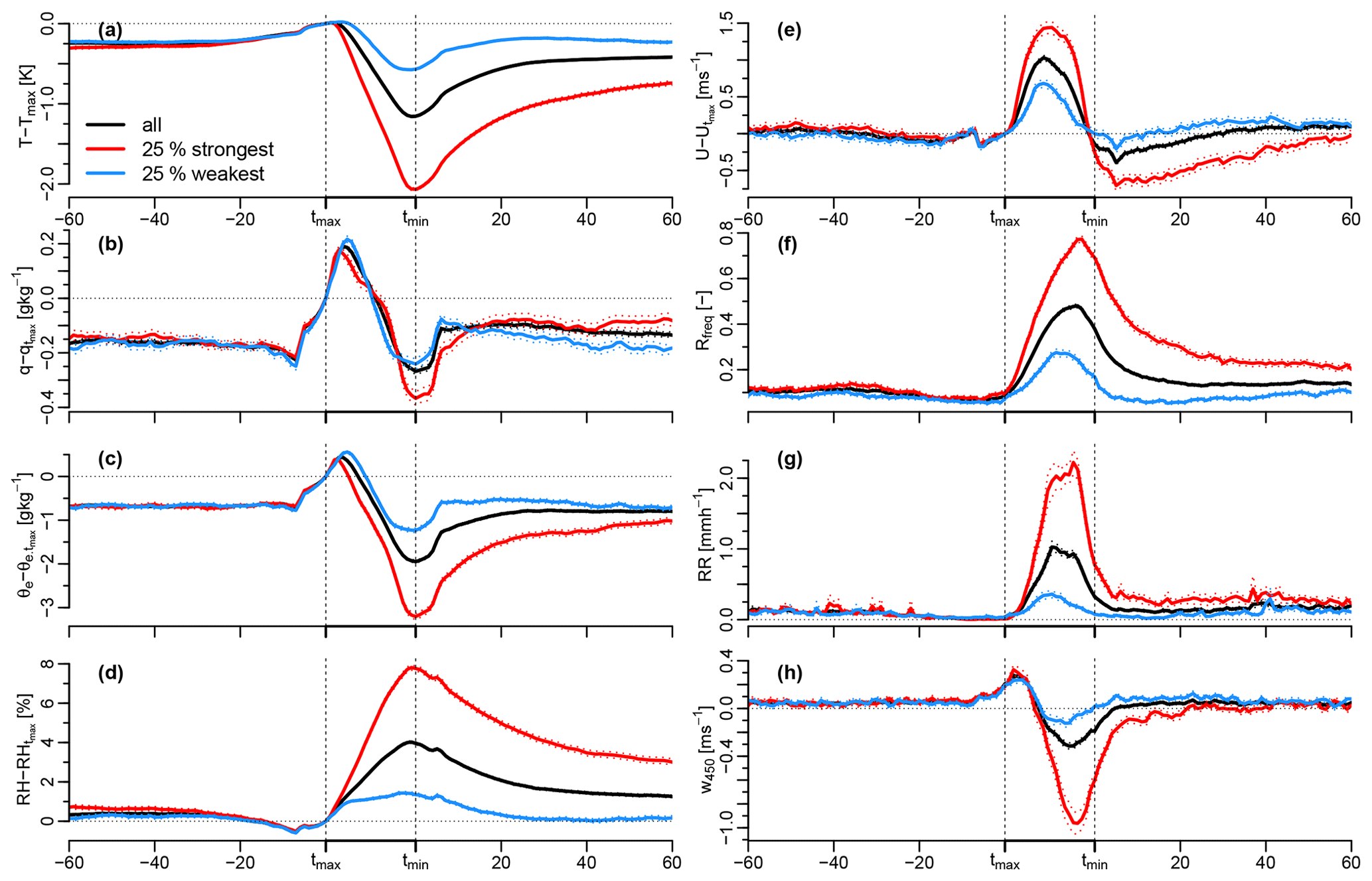
Figure 3 Composite mean temporal structure of anomalies with respect to the cold-pool onset (t_max) for the surface properties (a) temperature, (b) specific humidity, (c) equivalent potential temperature, (d) relative humidity, and (e) wind speed as well as absolute values of (f) the MRR rain frequency and (g) rain rate and (h) the vertical velocity at 450 m height. The black line shows the mean structure of all cold pools matching the noprevWI criterion, and the red and blue lines show the mean for the 25 % strongest and weakest cold pools, respectively. The dotted lines show the mean ± 1 SE. Vertical and horizontal reference lines are added to indicate t_max, t_min, and 0.

The temperature of the composite-mean cold pool, after increasing slightly before t_max, decreases rapidly in the front to −1.15 K and recovers by $\mathrm{\Delta }T/e$ within 16 min after t_min (not shown). The temperature remains about 0.5 K below T_max in the hour after the frontal passage. The temperature drop in the front of the 25 % strongest cold pools is by definition stronger but with a mean tendency of −0.070 K min⁻¹ also more than twice as abrupt compared to the weakest cold pools. The strongest cold pools also take longer to recover than the weakest ones.

The temporal structure of the specific humidity response is intriguing. The composite-mean humidity starts to increase already 8 min before t_max and increases by about 0.2 g kg⁻¹ until t_max. In the first quarter of the front, the humidity increases by another 0.2 g kg⁻¹ before it drops to its minimum of −0.25 g kg⁻¹ at t_min, which is hardly lower than the pre-front value. The specific humidity response of the strongest cold pools only differs significantly from the weakest cold pools at t_min, with the humidity drop at t_min being about −0.4 g kg⁻¹ and thus about twice as strong as the drop for the weakest cold pools. If the entire set of cold pools including the summer season with deeper convection is used, the strongest cold pools have a significantly weaker positive humidity anomaly at the beginning of the front and a significantly faster and stronger humidity reduction at t_min compared to the weakest cold pools (see Fig. B1c–d).

The humidity recovers much more quickly than the temperature and remains slightly elevated compared to its pre-front value in the hour after. The fast humidity recovery might be due to the trapping of surface moisture fluxes in the anomalously shallow mixed layer typically associated with cold pools (Touzè-Peiffer et al., 2021). Another reason in cases of more strongly precipitating cold pools might be continued evaporation of precipitation, which would cool and moisten the air in the cold-pool wake and thus speed up the humidity recovery but slow down the temperature recovery.

The initial increase in humidity at the edge of the front at the BCO might be explained by enhanced surface fluxes due to the strengthening winds (Langhans and Romps, 2015; Torri and Kuang, 2016), by moisture advection (Schlemmer and Hohenegger, 2016), or by an accumulation of moisture from evaporation of precipitation of the parent convection, which was pushed to the edge of the front (Tompkins, 2001). Analyses of the various isotope measurements made during the EUREC⁴A field campaign (Stevens et al., 2021) might help elucidate the origin of these moisture rings, as suggested by idealized large-eddy simulations (Torri, 2021). This could also help understand why cloud-resolving models seem to have difficulties in representing the humidity structure in the cold-pool front correctly (Chandra et al., 2018). As discussed by de Szoeke et al. (2017), the humidity increase just before t_max might be mostly due to the increasing saturation-specific humidity associated with the increasing temperature before t_max (as seen by the relative humidity anomaly in panel d being slightly below zero) and as such likely also related to the way we identify T_max. A potential dynamical reason for the pre-front humidity increase could be moisture convergence ahead of the front (Schlemmer and Hohenegger, 2016).

The temporal structure of the equivalent potential temperature (Fig. 3c) is similar to the humidity structure but with a stronger drop across the front and a stronger difference between the weaker and stronger cold pools governed by the temperature drops. The relative humidity signal in the front is mostly governed by the temperature decrease, with RH being 8 % larger at t_min for the strongest cold pools.

The in-front wind speed increase has a maximum in the middle of the front, confirming that the interval between t_max and t_min catches the front characterized by a vortical overturning internal circulation. After the frontal passage, the wind speed decreases slightly below the pre-front level. As the cold pools spread into a strong background easterly flow (mean wind direction at t_max is 86^∘, not shown), the wind speed anomalies show that the cold pools on average push forward into the wind until t_max, and backward after t_min. For some cold pools, t_min might thus mark the center of the divergent flow and indicate that the parent convection passed over the BCO. The strengthening winds in the front and the slackening winds in the wake are again significantly more pronounced for the strongest cold pools, with a maximum of 1.5 m s⁻¹ and a minimum smaller than −0.5 m s⁻¹ in the front and wake compared to the value at t_max.

Figure 3f–g show the composite mean R_freq and RR measured by the MRR. Both rain variables increase rapidly after the onset of the cold pool, peak towards the middle or end of the front, and start to decrease shortly before t_min. The strongest cold pools have much larger rain rates and rain frequencies during the entire front compared to the weakest cold pools, and the rain frequency of the strongest cold pools also remains strongly elevated until more than an hour after t_min.

The last panel of Fig. 3h shows the Doppler lidar vertical velocity averaged over four 30 m range gates with mean height of 450 m (w₄₅₀). The mean w₄₅₀ peaks at the edge of the front with about 0.25 m s⁻¹ and decreases rapidly to −0.3 m s⁻¹ near the end of the front, reflecting updrafts triggered at the cold-pool gust front and downdrafts driven by the evaporating precipitation inside the front, respectively. The median w_max450 at the gust front edge (see Table 1) is at 1 m s⁻¹ much larger than the averaged hourly in-cloud vertical velocities near cloud base measured by the BCO Doppler radar, which has a peak density at 0.2 m s⁻¹ and maxima of 0.6 m s⁻¹ (Klingebiel et al., 2021). 1 m s⁻¹ also marks the upper tail of cloud-base averaged updraft vertical velocities at the BCO (see Fig. 4b of Sakradzija and Klingebiel, 2020). This suggests that the gust-front vertical velocity maxima are very relevant for triggering new convection in the trade cumulus regime. The strongest cold pools have significantly stronger downdrafts and also updrafts compared to the weakest cold pools (see also Table 1), the latter highlighting the potentially enhanced triggering of new convection by stronger cold pools. For the vertical velocity averaged over the entire sub-cloud layer (w_SCL), the picture is similar, but the peak w_maxSCL is slightly smaller for the strongest cold pools and more similar compared to the weaker cold pools (Table 1).

As already shown in Table 1, Fig. 3 shows that the strongest cold pools are also the driest and the rainiest, and have the strongest wind and vertical velocity anomalies in the front. The relationships and timings discussed are mostly the same when considering all cold pools meeting the noprev criterion (i.e. also including summer periods), just with larger anomalies and the differences mentioned above for the humidity structure. The mean temporal structure for all variables – except for the specific humidity and partly for the wind speed – is also similar to previous observations of tropical deep convective cold pools during the DYNAMO field campaign (de Szoeke et al., 2017; Chandra et al., 2018), just with slightly larger mean across-front temperature and humidity decreases (−1.3 K and −0.6 g kg⁻¹ during DYNAMO compared to −1.15 K and −0.25 g kg⁻¹ at the BCO) and larger mid-front wind speed increases (about 1.5 m s⁻¹ compared to 1 m s⁻¹) during DYNAMO due to the deeper convection. Furthermore, during DYNAMO the increases in specific humidity at the beginning of the front are hardly present, and the wind speed remains elevated by 0.4 m s⁻¹ in the wake of the DYNAMO cold pools (de Szoeke et al., 2017), whereas at the BCO the wind speed decreases below the value at t_max in the wake. We hypothesize that this difference can be explained by the stronger cold pools during DYNAMO travelling further away from their parent convection, such that they continue to push forward into the mean wind. What strengthens cold pools in the trades despite the shallower parent convection is the drier cloud layer and free troposphere compared to the deep convective regions, which facilitates evaporation of precipitation and can strengthen downdrafts (Chandra et al., 2018).

The cloud radars at the BCO also allow study of how the cloud properties change across the cold-pool passage (Fig. 4). The mean cloud-top height (CTH) increases rapidly by ∼500 m after the cold-pool onset and peaks at the end of the front. CTH remains elevated by about 300 m compared to the pre-front value in the following hour. The 25 % strongest cold pools are associated with significantly deeper clouds throughout the entire period shown, especially so at the end of the front, when the CTH is on average higher than 3300 m. The cloud-base height (CBH) starts to decrease already slightly before t_max and reaches its minimum near the end of the front at ∼500 m. This decrease is due to the more frequent precipitation with very low echo-base heights and is most pronounced for the strongest cold pools.

Figure 4 (a–f) Same as Fig. 3 but for (a) cloud-top height, (b) cloud-base height, (c) total cloud cover, and the contribution to total cloud cover from (d) CC_prcp, (e) CC_lcl, and (f) CC_aloft. Also indicated is the climatological mean value for the winter periods of 2012–2020. (g–i) Composite mean temporal structure of vertical hydrometeor fraction (HF) profiles for all noprevWI cold pools as well as the 25 % strongest and weakest. The thin dashed line at 600 m height marks the typical base of the cumulus layer.

The total hydrometeor cover (CC) increases rapidly at the beginning of the cold-pool front, remains about 25 % larger compared to the pre-front value inside the front, and decreases slowly in the wake. The mean CC of the 25 % strongest cold pools reaches nearly 100 % at the end of the front and is significantly larger than the CC of the weakest cold pools during the entire period shown, especially so in the wake. In Fig. 4d–f the cloud cover is split into contributions from cloud segments with different CBH by considering all 1 min hydrometeor fraction profiles independently. This shows that the enhanced CC of the strongest cold pools in the prior hour is entirely due to cloud segments with CBH above 1 km (CC_aloft), whereas the enhanced CC in the front and wake of the strongest cold pools is mostly due to precipitating cloud segments with CBH below 300 m. The rapid increase in CC_lcl up to its peak at t_max strongly contributes to the CC increase at the edge of the front. This peak is also larger for the strongest cold pools, consistent with their larger w₄₅₀ at t_max. CC_lcl and CC_aloft are lower at the end of the front for the strongest cold pools, as the lowest CBH is mostly below 300 m and the cloud segments thus count to the CC_prcp category. (Note that a given time can only count to one of the three categories.)

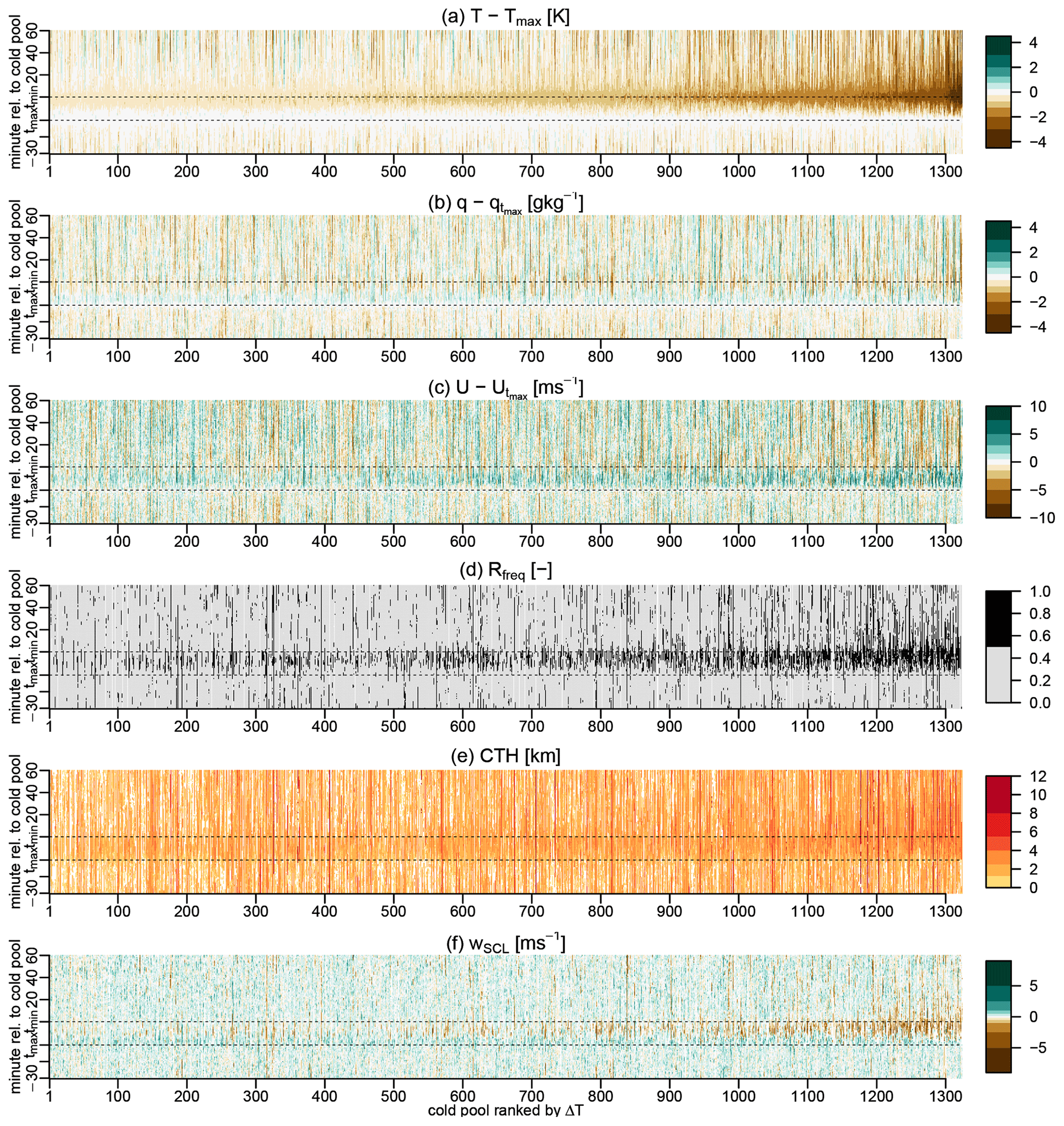
Figure 5 Temporal structure of individual cold pools ranked according to their ΔT. Shown are all cold pools of noprevWI that have all instruments running. The panels show anomalies relative to the cold-pool onset (t_max) for (a) temperature, (b) specific humidity, and (c) wind speed as well as absolute values of (d) the MRR rain frequency, (e) the cloud-top height, and (f) the vertical velocity averaged over the sub-cloud layer.

Overall, Fig. 4 indicates that clouds and rain are nearer t_min in the strongest cold pools and nearer t_max for the weakest cold pools. A potential explanation for this observation is that stronger cold pools are running further ahead of their stronger parent convection, while the weaker parent convection of the weaker cold pools might have already dissipated. However, drawing such conclusions from single-point observations is tricky, as the influence of the life-cycle stage and the overall cold-pool strength on the observed cold-pool characteristics cannot be disentangled. Some information about different cloud types populating the cold-pool front or wake can be derived by analysing the CC contributions grouped by the overall CBH of the segmented cloud objects (CBH_ID; see Appendix A and Sect. 2.1). We find that the peak in CC_lcl at t_max is mainly due to edges of precipitating clouds that have CBH > 300 m. Assuming that this cloud population represents the clouds evident as mesoscale arcs in satellite imagery, this suggests that the cloudiness at the gust front is mostly characterized by well-developed precipitating clouds. The cloud-type analysis also shows that more than half of the CC_aloft in the cold-pool wake is part of large precipitating clouds and is not from detached stratiform layers. This is also suggested by the time–height plots of the composite-mean hydrometeor fraction shown in Fig. 4g–i. These panels nicely summarize what was discussed in the previous paragraphs and again highlight the differences between the 25 % strongest and weakest cold pools in terms of the cloud response.

Figure 4a–f also indicate the respective mean CTH, CBH, and CC for all the winter months of the period 2012–2021. They show that cold-pool periods are much cloudier than the average winter conditions at the BCO, with the average in-front CC being twice as large as the 10-year climatological mean. Cold-pool periods also have much deeper clouds than the climatological mean of about 2 km, which is expected as it needs deeper precipitating clouds to form cold pools. The enhanced CC in the wake of cold pools compared to the long-term mean is nevertheless surprising, as convection might be expected to be suppressed in the cold-pool wake. Mesoscale arcs encircling vast decks of deeper cumuli with stratiform layers therefore seem more representative for periods of cold-pool activity than the more classical picture of trade cumulus cold pools as mesoscale arcs enclosing broad clear-sky areas.

Despite the various significant differences between the strongest and weakest cold pools highlighted in the previous paragraphs, there is a lot of variability among individual cold pools. The variability is illustrated in Fig. 5, which shows the temporal structure of the most important variables for individual cold pools ranked according to their ΔT. Especially the individual differences in humidity and wind in the front and beginning of the wake can by far exceed the mean differences among the strongest and weakest cold pools shown in Fig. 3. Notable is again the occurrence of pronounced negative values of the wind speed anomaly after t_min, which suggests that some cold pools push backward into the mean wind. Tendencies of more frequent (and intense) rain, deeper clouds, and stronger downdrafts near t_min of the stronger cold pools are nevertheless clearly evident. Especially the downdraft strength seems to be systematically increasing for stronger temperature drops. Besides showing the CTH, Fig. 5e also gives an indication of the CC, again illustrating how cloudy the cold-pool periods are.

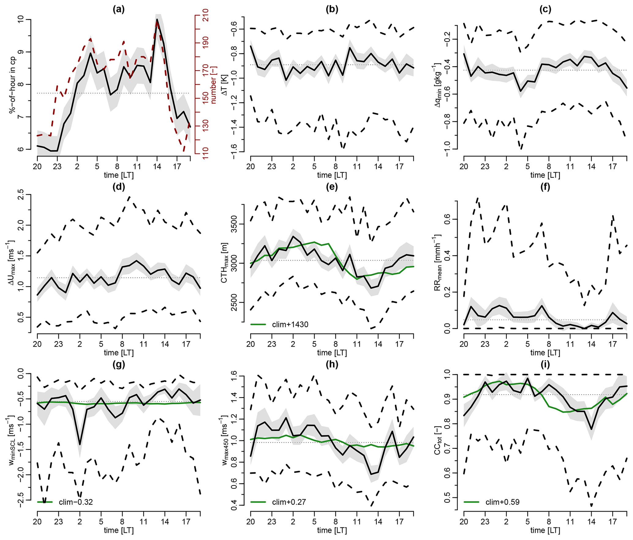
Figure 6 Daily cycles of important cold-pool diagnostics. (a) Mean ± 1 SE of hourly cold-pool frequency as well as the number of cold pools per hour, (b) ΔT, (c) Δq_min, (d) ΔU_max, (e) CTH_max, (f) MRR RR_mean, (g) w_minSCL, (h) w_max450, and (i) CC_tot, with cold pools associated with a specific hour according to their t_max. In panels (b)–(i) the lines represent the 25 %, 50 %, and 75 % quartiles of the respective variables and the shading represents the median ± 1 SE. Also indicated in green is the median climatological background diel cycle of 30 min values of (e) maximum CTH, (g) minimum w_SCL, (h) maximum w₄₅₀, and (i) mean CC, shifted by the mean difference of the climatological median compared to the cold-pool median to ease reading. Due to the infrequent rain, the median climatological RR_mean is always 0 and omitted in panel (f).

3.3 Diel cycle

The long time series also allows study of the variability of the cold-pool frequency and characteristics at the daily timescale. Figure 6 shows the diel variability of cold-pool properties for the noprevWI set. There are clearly fewer cold pools and a lower hourly cold-pool frequency between 16:00 and 22:00 LT compared to the rest of the day. Just before midnight, the cold-pool frequency strongly increases in response to the nighttime increase in cloud cover, cloud depth, and rain rate (see green lines in panels e–i and Vial et al., 2019). The cold-pool occurrence remains strongly elevated between 02:00 and 15:00 LT, with a peak at 14:00 LT.

Also, most cold-pool diagnostics show a pronounced diel variability. During nighttime between about midnight and 04:00 LT, cold pools are associated with significantly deeper clouds, stronger mean rain rates, stronger downdrafts and updrafts, larger CC, and slightly stronger humidity drops and weaker wind gusts compared to daytime cold pools between about 08:00 and 16:00 LT. There is also a hint of slightly stronger ΔT during nighttime compared to daytime, but neither in the median nor in the 25 % quartiles is this diel cycle significant. It is somewhat surprising that we find no pronounced diel cycle in ΔT, despite the diel cycle of e.g. w_minSCL and CTH_max. There is a climatological background diel cycle in temperature of about 1.2 K due to the daytime solar heating of the ground at the BCO (minimum and maximum temperatures near 05:00 and 12:00 LT, respectively, not shown), but this should not affect the cloudy cold-pool periods much and would contribute to lower ΔT in the morning. Other diagnostics like Δq_max and R_int do not show a pronounced diel variability (not shown).

The pronounced diel variability in the cold-pool frequency and most diagnostics is not surprising given the distinct diel cycle in trade cumulus cloudiness discussed in detail in Vial et al. (2019) based on realistic high-resolution simulations and both BCO and satellite observations. The diel cycle of trade cumuli is characterized by larger CC and deeper clouds at the end of the night and smaller CC and shallower clouds in the afternoon. This is evident in the background climatological diel cycles indicated in Fig. 6e–i. The diel cycles of most cold-pool diagnostics have a similar phase and also amplitude to their background diel cycles but are shifted to much larger values (as indicated in the respective legends). For the vertical velocity diagnostics, the amplitude of the diel cycle is also much larger compared to the background climatology.

The period of enhanced cold-pool occurrence between 23:00 and 15:00 LT and its peak at 14:00 LT extends much further into the day compared to the period of enhanced mean background rain rate between about 03:00 and 06:00 LT typical for the trades (Nuijens et al., 2009; Vial et al., 2019), suggesting that cold pools help extend the diel cycle of shallow convection into the early afternoon. Also, the diel cycle of cloud cover seems to be slightly extended in cold-pool periods, with CC_tot decreasing below the diel mean about 4 h later compared to the climatological CC. The likely reason for the extension of convection into the afternoon is that the cold pools are successful in triggering new convection, which can again induce new cold pools that trigger further convection. Thereby, cold pools reinforce each other, which is supported by the shorter median interval between subsequent cold pools of 121 min between 07:00 and 14:00 LT compared to 182 min between 22:00 and 04:00 LT.

The importance of cold pools in triggering new convection is well established in the literature and can occur through mechanic lifting or moisture accumulations, both of which are favoured when multiple cold pools collide (Rotunno et al., 1988; Tompkins, 2001; Feng et al., 2015; Torri and Kuang, 2019; Meyer and Haerter, 2020). Rochetin et al. (2021) also found a diel cycle of cold-pool occurrence near Barbados in realistic simulations with the ICON model at 2.5 km grid spacing, however, without the pronounced extension into the afternoon observed at the BCO (see their Fig. 16d). This might be due to gust front vertical velocities being poorly resolved at kilometre-scale resolutions, which leads to too little convective triggering and deficits in rain and convective organization, as simulations over Germany showed (Hirt and Craig, 2021).

Vial et al. (2021) also find the diel cycle of trade cumuli to be strongly linked to the diel cycle in the occurrence frequency of the mesoscale organization patterns. Whether the cold-pool characteristics and their diel cycles are related to the pattern of mesoscale organization will be discussed in the next section.

4 Relationship of cold-pool characteristics with mesoscale organization patterns

In this section we investigate whether the cold-pool frequency and characteristics depend on the pattern of mesoscale cloud organization. For this we condition the cold pools on the organization pattern present at the BCO. As explained in Sect. 2.2, a cold pool is attributed to a pattern if it is present during >75 % of the cold-pool duration. As multiple patterns can be present at the same time, two (or rarely even three) patterns can be attributed to one cold pool. Pattern labels are available from January 2018 to March 2021, and using the noprevWI criterion leaves 1332 cold pools to be analysed.

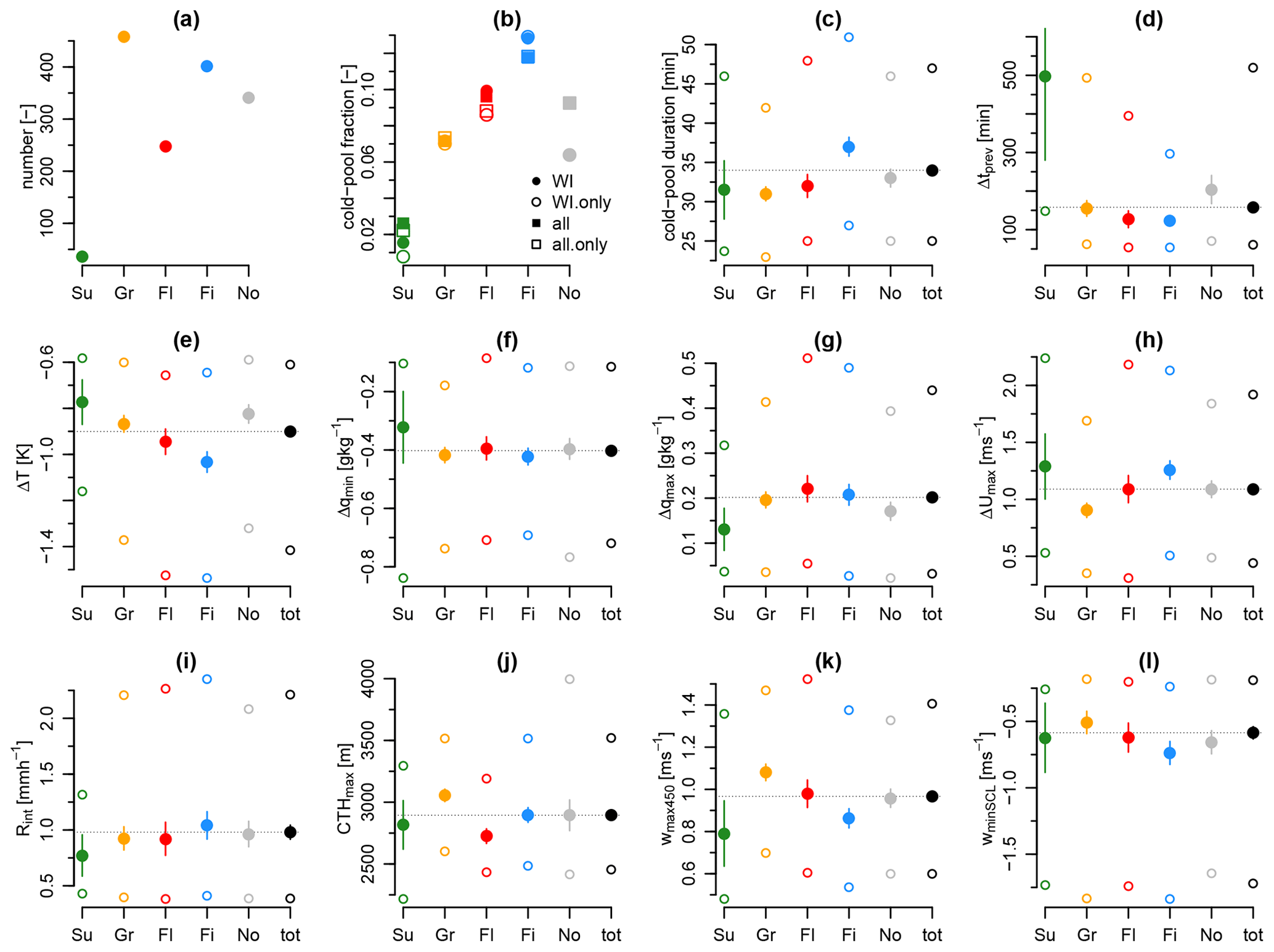
Figure 7 Distributions of various cold-pool diagnostics conditioned on the organization patterns. (a) Number of cold pools, (b) cold-pool fraction, (c) cold-pool duration, (d) time since t_min of the last cold pool, (e) ΔT, (f) Δq_min, (g) Δq_max, (h) ΔU_max, (i) MRR R_int, (j) CTH_max, (k) w_max450, and (l) w_minSCL. The different symbols in panels (c)–(l) represent the 25 %, 50 %, and 75 % quartiles of the respective variables, the solid lines represent the median ± 1 SE, and the dotted horizontal reference lines show the median of the entire set (“tot”). Besides the cold pools matching the noprevWI criterion, panel (b) also shows the fraction of cold pools for all seasons (“all”) and excluding periods with multiple organization patterns (“WI.only” and “all.only”).

The discussion of the 4 example cold-pool days in Fig. 2 already shed some light on the differences in the cold-pool characteristics of the four patterns. For a statistical comparison, Fig. 7 shows distributions of several cold-pool properties for the different patterns, including the “No” category and the union of the five categories (“tot”). The most pronounced difference among the patterns lies in the occurrence frequency of cold pools. Most cold pools detected at the BCO pertain to the Gravel pattern, followed by Fish and Flowers (Fig. 7a). As expected, only a few cold pools are detected during Sugar periods. Many cold pools are also associated with the No category.

When we look at the fraction of time a cold pool is observed in a given pattern (Fig. 7b), the picture changes and the Fish pattern is associated with the largest cold-pool fraction (12.8 % of the time), followed by Flowers and Gravel (9.9 % and 7.2 %, respectively). Again, Sugar has clearly the lowest cold-pool fraction (1.6 %). The cold-pool fraction of the No category in winter is at 6.4 % also substantial. Figure 7b also shows the cold-pool fractions using different selection criteria, namely that cold pools attributed to multiple patterns are excluded (“.only”) and that all noprev cold pools from all seasons are used (“all”). The four patterns remain distinct in their cold-pool fractions independent of the criteria considered. Only for Sugar (and to a small extent also Flowers) do these criteria change the cold-pool fraction. The No category is particularly sensitive to the inclusion of all seasons, as in summer with more frequent deep convection most cold pools pertain to the No category (not shown).

That Gravel has the largest number of cold pools but only the third largest cold-pool fraction is partly because Gravel is the most frequent pattern at the BCO (a total of 178 d out of the 18 winter months considered, compared to 113 Fish, 78 Flowers, and 72 Sugar days) and partly because Gravel cold pools on average last 6 min shorter than Fish cold pools (Fig. 7c). Fish has the significantly longest-lasting cold pools of all patterns, which is tightly linked to frequent long-lasting rain events. Cold pools in the Fish pattern also follow each other most rapidly, with a median of 124 min separating individual cold pool fronts (Fig. 7d). Also for Flowers and Gravel, cold pools follow each other quickly, whereas much more time passes between cold pools for Sugar and No. The same picture emerges when considering the cold-pool length (i.e. the duration multiplied by the surface wind speed): Fish cold pools are with a median size of 13.8 km slightly larger than Gravel and Flowers cold pools (both about 12.6 km, not shown).

Figure 7e–i show the differences in the surface meteorology, rain, and cloud response associated with cold pools for the different patterns. Fish has the strongest median ΔT and the strongest downdrafts of all patterns (Fig. 7e, l) and also a stronger ΔU_max compared to Gravel and Flowers (Fig. 7h). Gravel cold pools are associated with significantly larger CTH_max and stronger updrafts compared to the other patterns (Fig. 7j, k). For the humidity and rain diagnostics (Fig. 7f, g, i), the differences between Gravel, Flowers, and Fish cold pools are minor. Sugar cold pools generally have the weakest cold-pool signatures. Contrastingly, the cold pools of the No category show no significant differences compared to Gravel, Fish, and Flowers for most statistics. These results are largely insensitive to both an increase in the neural network agreement score (i.e. using 0.5 compared to 0.4; see Sect. 2.2) and to the exclusion of multiple patterns (except for Sugar and to some degree also Flowers, whose sample sizes become very small, not shown).

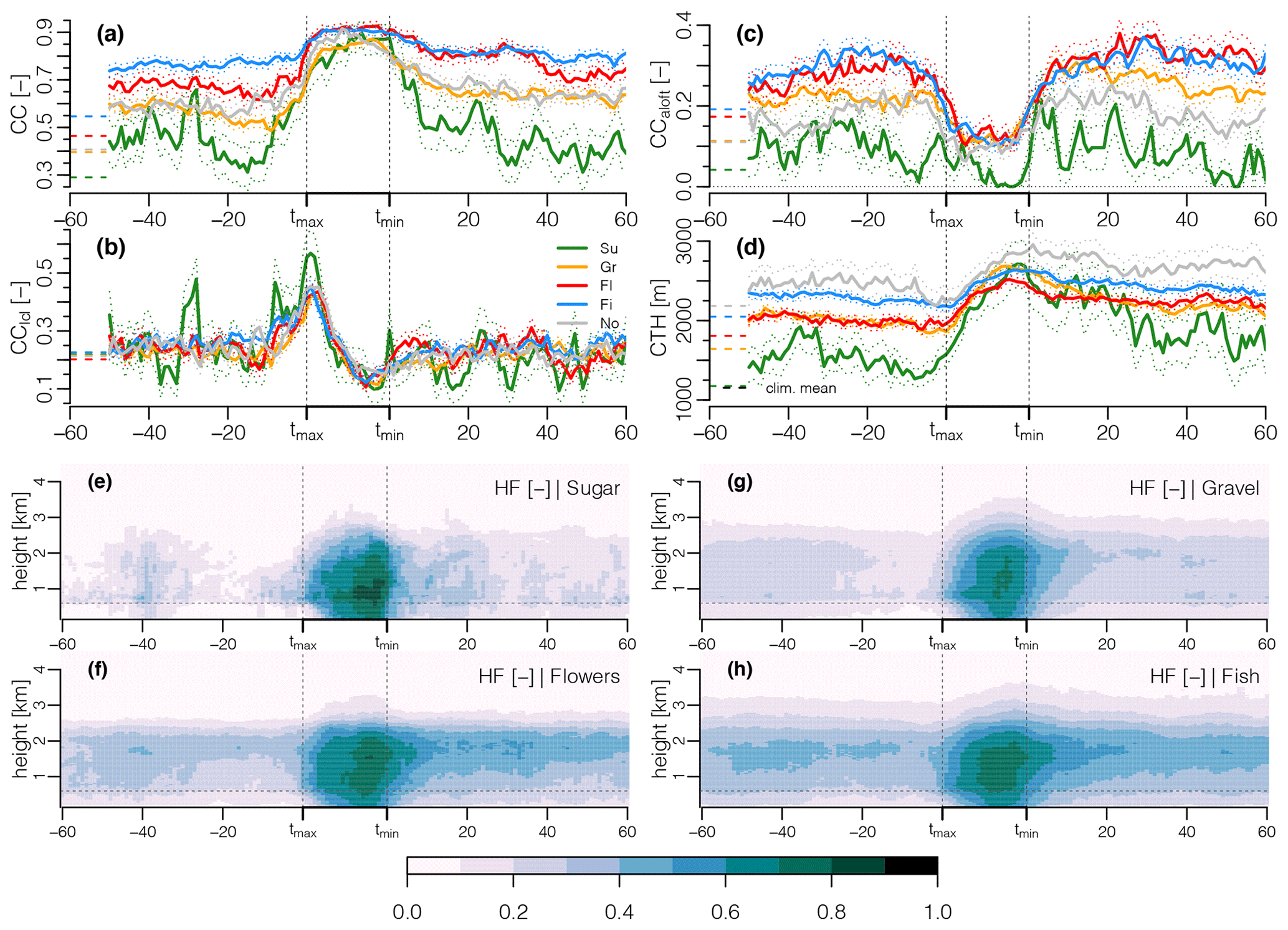
Figure 8 Composite mean temporal structure of the four organization patterns and the No category. Shown are (a) total CC, the contribution to total CC from (b) CC_lcl and (c) CC_aloft, and (d) the CTH. The dotted lines show the mean ± 1 SE. Also indicated on the far left of panels (a)–(d) are the climatological mean values per pattern for the corresponding winter periods of 2018–2021. Panels (e)–(h) show the mean temporal structure of the vertical hydrometeor fraction profiles for the four patterns.

Figure 8 shows the differences in the temporal structures of cloud properties associated with the cold-pool passages for the four patterns. Fish and Flowers have the largest CC (Fig. 8a) due to larger contributions of CC_aloft (Fig. 8c), which are associated with frequent stratiform layers near 1.5–2 km (Fig. 8f, h). CC_lcl (Fig. 8b) and CC_prcp (not shown) instead are fairly similar among the patterns. The CC of Fish cold pools hardly changes across the cold-pool passage, whereas the onset of the cold-pool front is much more clearly evident for the Gravel and even more for the Sugar CC (see also the time–height composites in Fig. 8e–h). The CC in the wake of Sugar cold pools also decreases most rapidly back to its pre-front value. Fish tends to have the deepest mean CTH associated with the cold-pool periods, closely followed by Gravel and Flowers. Again, the mean CTH of Gravel and Sugar cold pools increase most rapidly in the front compared to the other patterns.

For all patterns, the cold-pool periods are characterized by significantly deeper clouds and larger CC compared to the pattern average (indicated by the dashed lines on the far left of Fig. 8a–d). Nevertheless, the climatological differences in CC, CC_aloft, and CTH among the different patterns (Schulz et al., 2021; Vial et al., 2021; Bony et al., 2020) also remain during cold-pool periods, indicating the robustness of the pattern-specific cloud macrophysical properties. The climatological differences in CTH of the patterns correspond very well to their differences in the cold-pool fraction (Fig. 7b), with Sugar having clearly the shallowest mean CTH and the lowest cold-pool fraction, separated by a step change from Gravel, followed closely by Flowers and Fish. The two patterns with the largest cold-pool fraction, Fish and Flowers, also have the largest mean cloud object sizes (Bony et al., 2020), suggesting that cloud size and cold-pool occurrence are positively correlated (Schlemmer and Hohenegger, 2014).

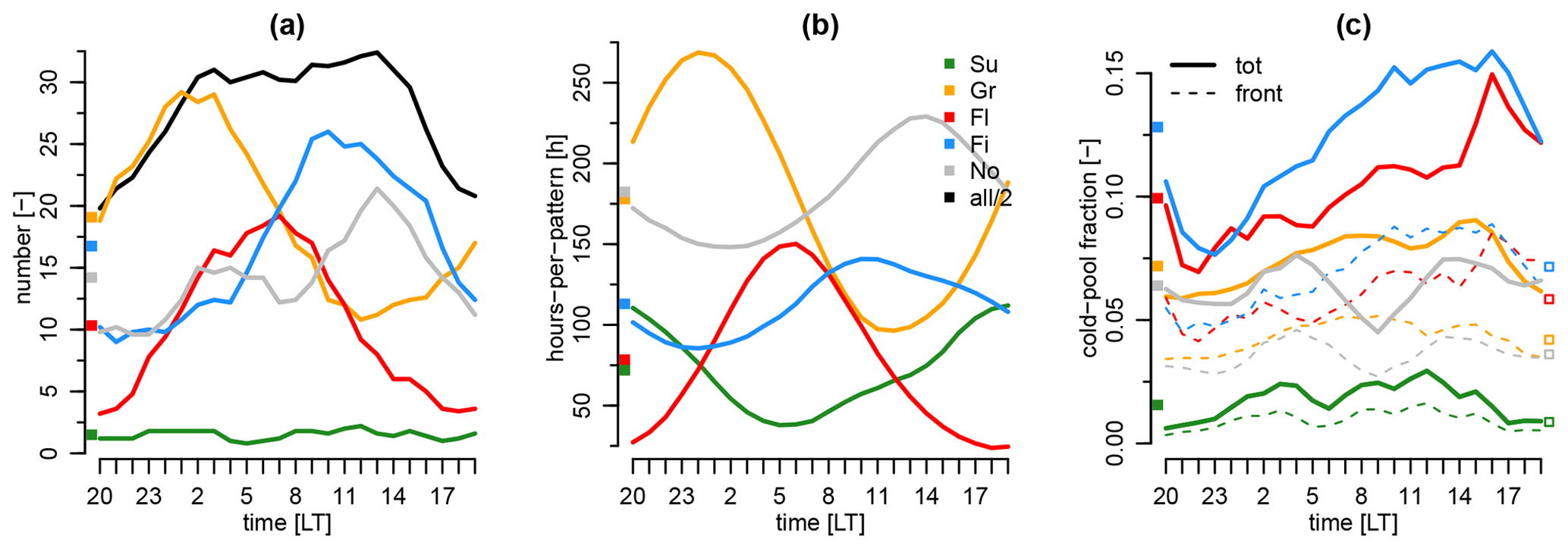
Figure 9 Daily cycles of (a) number of cold pools, (b) hours of data for the different organization patterns, and (c) hourly fraction in cold pool (solid) and in cold-pool front (dashed). A 5-hourly running mean is applied to smooth the data. The diel means are indicated on the left-hand side of each panel.

As mentioned before, Vial et al. (2021) find the diel cycle of trade cumuli to be strongly linked to the diel cycle in the occurrence frequency of the mesoscale organization patterns. Figure 9a shows strong diel variations of the number of cold pools associated with the different patterns. These variations are strongly connected to the diel cycles in the occurrence frequency of the patterns (Fig. 9b and Vial et al., 2021). The maximum number of Gravel cold pools occurs just after midnight, followed by Flowers around 07:00 LT and Fish cold pools at 10:00 LT. The number of Sugar cold pools is very low throughout the day.

Figure 9a suggests that the extension of the diel cycle of convection into the early afternoon due to cold pools may largely be explained by the Fish pattern, together with a substantial contribution of the No category to the peak at 14:00 LT. Despite the strong connection between the diel phasings of Fig. 9a–b, especially the Fish pattern also shows a diel cycle of the cold-pool fraction with a peak in the afternoon (Fig. 9c), which is broadly in phase with the occurrence frequency. The diel cycle in the cold-pool fraction might be due to cold pools lasting a while once they are formed, which is supported by the much weaker diel cycles of the cold-pool front fraction (dashed lines in Fig. 9c). Once present, cold pools often trigger new cold pools, as suggested by the 33 % shorter interval between subsequent fronts during daytime compared to nighttime (see discussion in Sect. 3.3). From the present analyses, it is difficult to disentangle causal relationships between the pattern occurrence, cold pools, and the diel cycle. It is also difficult to pin down the evolution from one pattern to another and the role of cold pools therein. As the number of cold pools per pattern and hour is quite low (especially in the case of Flowers), more data are needed to draw robust conclusions on this.

The pattern-associated diel phasing of the cold-pool number might give a clue about why ΔT varies little on the daily timescale (Fig. 6c), although the diel cycle of most cold-pool properties would suggest that ΔT should be stronger at night compared to day. The daytime Fish pattern has significantly stronger ΔT compared to the nighttime Gravel pattern (Fig. 7e), which might compensate for the opposite expectation due to the diel phasing of CTH_max and w_minSCL.

5 Conclusions

This paper presents a long-term climatology of trade cumulus cold pools based on more than 10 years of in situ and ground-based remote sensing data from the Barbados Cloud Observatory (BCO; Stevens et al., 2016). Cold pools are detected by abrupt drops in low-pass-filtered temperature time series, and their associated changes in surface meteorology, cloudiness, and sub-cloud layer dynamics are extracted. The cold-pool climatology is combined with a neural network classification of the four mesoscale organization patterns Sugar, Gravel, Flowers, and Fish (Stevens et al., 2020) based on GOES-16 ABI infrared images (Schulz et al., 2021). To focus on trade cumulus cold pools, most analyses are restricted to the set of 3889 cold pools detected in the dry winter regime from December to April that have no non-recovered cold pool in the hour prior to their onset.

We find cold pools to be ubiquitous in the winter trades – they are present about 7.8 % of the time, and on more than 73 % of days at least one cold pool is detected. The average cold-pool passage is characterized by a 0.9 K temperature drop, a 0.2 g kg⁻¹ humidity increase just before and another 0.2 g kg⁻¹ humidity increase right after the front onset, followed by a −0.4 g kg⁻¹ humidity decrease at the end of the front, wind speed and pressure increases of 1.15 m s⁻¹ and 9 Pa, and rain intensities of 0.9 mm h⁻¹. The vertical velocity at the sub-cloud layer top shows pronounced maxima of 1 m s⁻¹ near the cold-pool onset, which lies in the upper tail of cloud-base averaged updraft velocities at the BCO (Sakradzija and Klingebiel, 2020) and thus is very relevant for triggering new convection. The second half of the front is marked by sub-cloud layer averaged downdrafts of −0.55 m s⁻¹. Strong signals of cold-pool passages are also found for all cloud macrophysical properties analysed: cloud-top height increases, cloud-base height decreases (due to the very frequent precipitation), and cloud cover increases with the cold-pool onset. Cloudiness at the gust front is mostly due to cloud segments near the lifting-condensation level that pertain to larger precipitating cloud objects. Similarly, cloud segments with bases above 1 km in the cold-pool wake are mostly part of large precipitating clouds and are not from detached stratiform layers.

The strength of the cold-pool signature depends strongly on the intensity of the temperature drops (ΔT). The rain duration in the front is the best predictor of ΔT and explains 36 % of its variability. We find that the minimum vertical velocity averaged over the sub-cloud layer and the maximum cloud-top height also distinguish stronger and weaker cold pools very well. Cold pools with stronger ΔT are associated with deeper clouds, stronger precipitation, downdrafts, and humidity drops, stronger wind gusts and updrafts at the edge of the front, and larger cloud cover compared to cold pools with weaker ΔT. Stronger cold pools also last significantly longer and follow each other more quickly than weaker cold pools, indicating that they are likely more successful in triggering new convection than weaker cold pools. We find clouds and rain to be nearer to the temperature minimum in the strongest cold pools, whereas they tend to be nearer the onset of the front in weaker cold pools. This suggests that stronger cold pools are running further ahead of their stronger parent convection, while the clouds forming the weaker cold pools might have already dissipated.

The cold-pool frequency and characteristics show pronounced diel variability. There are significantly fewer cold pools and a lower cold-pool frequency between 16:00 and 22:00 LT compared to the rest of the day. We find that cold pools extend the diel cycle of convection into the early afternoon, with a peak in both the cold-pool number and fraction at 14:00 LT. Also, most cold-pool diagnostics show a pronounced diel cycle, with significantly deeper clouds, stronger mean rain rates, stronger downdrafts and updrafts, larger cloud cover, slightly stronger humidity drops, and weaker wind gusts associated with nighttime compared to daytime cold pools. The phase of these diel signatures is consistent with their background climatological diel cycle but shifted to much larger values. The diel amplitude of the vertical velocity maxima and minima is also greater during cold-pool periods.

In the wet summer regime, cold pools are about 30 % more frequent relative to the average winter regime. Summer cold pools are also associated with significantly stronger temperature and humidity drops, deeper clouds, and stronger downdrafts – consistent with the frequent deep convection and stronger precipitation of this season (Brueck et al., 2015). On the other hand, the summer cold pools have weaker updrafts and humidity maxima at the beginning of the front, suggesting that they might be less effective in triggering new convection. While the temporal structures of cold-pool passages for most meteorological variables in both seasons resemble those of previous observations of tropical deep convective cold pools (de Szoeke et al., 2017; Chandra et al., 2018; Zuidema et al., 2017), especially the humidity structure and also the generally larger anomalies render the summer cold pools more similar to the deep convective cold pools from previous studies.

We also analysed whether the cold-pool frequency and characteristics depend on the pattern of mesoscale cloud organization. The most pronounced difference among the patterns lies in the occurrence frequency of cold pools, with Fish having the largest cold-pool fraction (12.8 % of the time), followed by Flowers and Gravel (9.9 % and 7.2 %, respectively). As expected, the cold-pool fraction of Sugar is negligible (1.6 %). Fish cold pools last significantly longer than cold pools from all the other patterns, and they are also associated with the strongest temperature drops and downdrafts. Gravel cold pools are associated with the strongest updrafts at the cold-pool onset and the deepest cloud-top height maxima.

Given the distinct diel cycle in the occurrence frequency of the four patterns found in Vial et al. (2021), it is not surprising that we find strong diel variations of the number of cold pools associated with the different patterns. The maximum number of Gravel cold pools occurs around midnight, followed by Flowers around 07:00 LT and Fish cold pools around 10:00 LT, in line with the diel cycles in the occurrence frequency of the patterns. The Gravel, Flowers, and Fish cold pools can thus explain a large fraction of the diel cycle in the cold-pool occurrence as well as their extension into the early afternoon. Note also that the unclassified cold pools have a non-negligible contribution to the peak at 14:00 LT. Interestingly, the climatological differences in the cloud cover and cloud-top height among the different patterns are also present during cold-pool periods – the overall cloud cover and cloud-top height for all patterns are just enhanced compared to their respective climatological values.

This study paves the way for more in-depth analyses of the cold-pool properties and their relation to the environment in the trades. Especially the complex humidity signals deserve a more detailed investigation, also using data from the recent EUREC⁴A field campaign (Stevens et al., 2021) and from realistic large-eddy simulations. Together with the vertical velocity statistics, the humidity anomalies can help shed light on the triggering of new convection at the cold-pool front. Additional measurements of the mixed-layer depth from radiosondes and the Raman or Doppler lidar could help refine the cold-pool end definition, which is only poorly constrained by the surface temperature data. Such additional data could also provide interesting insight into the cold-pool recovery process. A systematic matching with satellite imagery would also help collocate the clouds sampled at the BCO with the broader view of the entire cold pool seen from space.

Overall, we find that the cold-pool periods are about 90 % cloudier relative to the average winter trades. The larger cloudiness is mostly due to larger cloud cover from precipitating and stratiform cloud segments. Also, the wake of cold pools is characterized by above-average cloudiness, indicating that the classical image of trade cumulus cold pools as mesoscale arcs enclosing broad clear-sky areas is rather the exception than the rule. Our study suggests that a better understanding of how trade cumulus cold pools interact with and shape their environment is important for understanding the variability in cloud cover and cloud organization in the trade-wind regime.

Appendix A: Cloud cover contributions from different types of cloud objects

The contributions to total cloud cover from clouds at different height levels can either be computed by classifying every radar profile independently based on its CBH (see Fig. 4d–f) or – if a cloud segmentation mask is available – by classifying the entire cloud objects according to their CBH_ID (i.e. their overall lowest CBH). As both approaches can provide valuable insights, Fig. A1 also shows the temporal structure of the cold-pool signatures for the latter classification method. For this, the cloud cover is again split up into contributions from precipitating clouds with CBH_ID ≤ 300 m (CC_ID.prcp), LCL clouds (CC_ID.lcl; 300 m < CBH_ID ≤ 1 km), and stratiform clouds (CC_ID.aloft; 1 km < CBH_ID ≤ 4 km). The difference between CC_ID.prcp and CC_prcp is that edges or slanted sides of precipitating clouds that have a CBH > 300 m are counted in their entirety to the CC_ID.prcp category, while they would be counted in the CC_lcl or CC_aloft category if the cloud ID was not considered. Due to the potential presence of cloud objects at different heights, the sum of the three height categories (CC_ID.tot) can be larger than 1.

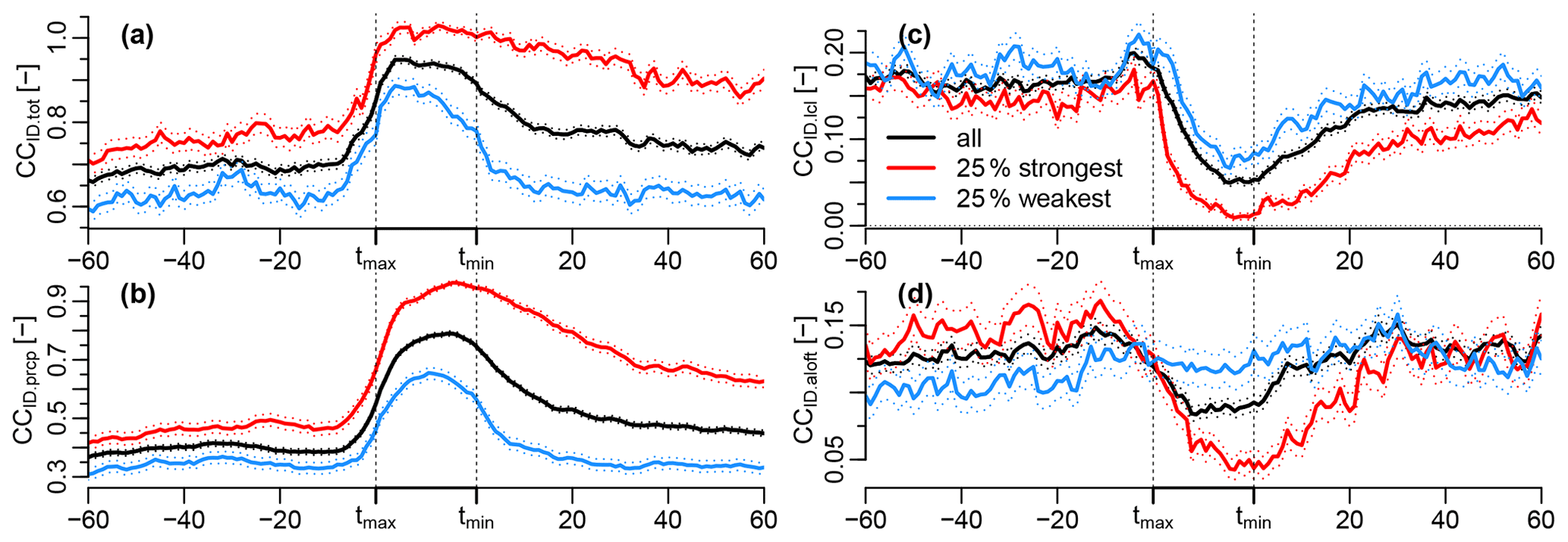
Figure A1 Same as Fig. 3 but for (a) CC_ID.tot, (b) CC_ID.prcp, (c) CC_ID.lcl, and (d) CC_ID.aloft for all cold pools of noprevWI and the 25 % strongest and weakest cold pools.

CC_ID.prcp already starts to increase before t_max and continues to increase until the middle of the front for all the cold-pool sets shown. For the 25 % strongest cold pools, the end of the front is entirely covered by precipitating clouds. CC_ID.lcl in Fig. A1c for all sets is relatively stable at about 17.5 % before the cold-pool onset, decreases abruptly after t_max to a minimum near t_min, and then slowly recovers back to the pre-front value. CC_ID.lcl shows the strongest impact when the cloud objects are considered through the CBH_ID and thus the strongest difference to the structure of CC_lcl (Fig. 4e). The absence of a peak in CC_ID.lcl near t_max indicates that the CC_lcl peak there is almost entirely due to edges of precipitating clouds with a CBH > 300 m and not due to (not-yet or) non-precipitating trade cumuli.

The temporal structure of CC_ID.aloft resembles the structure of CC_aloft (Fig. 4f) yet with substantially lower coverage, as most cloud segments with CBH > 1 km are connected to a precipitating core. This shows that nearly half of the CC_aloft in the cold-pool wake is part of large precipitating clouds and not from detached stratiform layers.

Appendix B: Seasonal cycle of cold-pool characteristics

While this study focuses on the cold-pool climatology of the winter regime, it is also interesting to look at the seasonal cycle of the cold-pool characteristics at the BCO. Using all cold pools of the noprev category, we find the largest median daily cold-pool frequency in the summer months from July to November and another peak in January (Fig. B1a). Only 13 % of days have no cold pool at all in summer, compared to 27 % in winter. The same monthly variability is found for the cold-pool front frequency but with 45 % lower values due to the shorter duration of the front compared to the entire cold pool (not shown).

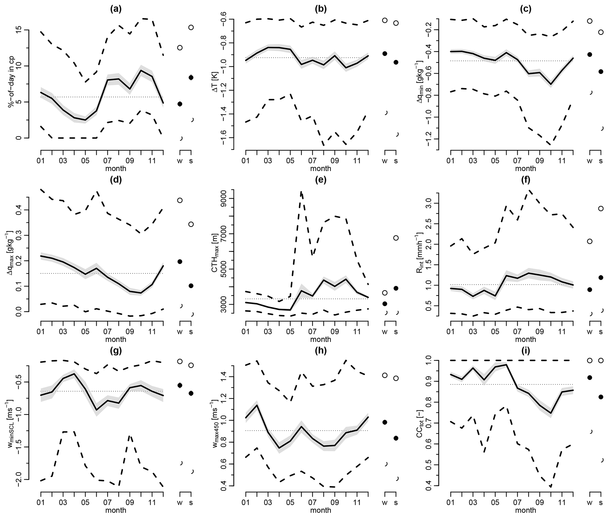
Figure B1 Monthly and seasonal distribution of important cold-pool diagnostics. (a) Daily cold-pool frequency, (b) ΔT, (c) Δq_min, (d) Δq_max, (e) CTH_max, (f) MRR R_int, (g) w_minSCL and (h) w_max450, and (i) CC_tot. The lines represent the 25 %, 50 %, and 75 % quartiles of the respective variables, the shading represents the median ± 1 SE, and the points show the average distribution for the 5 winter (w; December–April) and summer months (s; July–November).

Figure B1b–i show the monthly distributions of various cold-pool properties as well as averages over the 5 winter and summer months, respectively. They show that the summer cold pools are on average characterized by significantly stronger Δq_min, CTH_max, and R_int as well as slightly stronger ΔT and w_minSCL, consistent with the relationships discussed in Sect. 3. However, w_max450 is significantly lower by 0.2 m s⁻¹ and Δq_max by 0.1 g kg⁻¹ in summer compared to winter, indicating that cold pools in summer might be less successful in triggering new convection. Furthermore, CC_tot of summer cold pools is also significantly smaller compared to winter cold pools by about 10 %. The differences in the cold-pool characteristics between the summer and winter regimes are not surprising, as the summer regime is referred to as the wet season in Barbados and characterized by frequent deep convection and much larger precipitation (Brueck et al., 2015). When excluding periods of deep convection (defined by the presence of a radar signal between 4.5 and 8 km), the number of cold pools detected in summer strongly decreases compared to winter, and the median summer cold pool also becomes weaker compared to the median winter cold pool (not shown).