Spatially and temporally resolved measurements of NO_x fluxes by airborne eddy covariance over Greater London

Flux measurements of nitrogen oxides (NO_x) were made over London using airborne eddy covariance from a low-flying aircraft. Seven low-altitude flights were conducted over Greater London, performing multiple overpasses across the city during eight days in July 2014. NO_x fluxes across the Greater London region (GLR) exhibited high heterogeneity and strong diurnal variability, with central areas responsible for the highest emission rates (20–30 mg m⁻² h⁻¹). Other high-emission areas included the M25 orbital motorway. The complexity of London's emission characteristics makes it challenging to pinpoint single emissions sources definitively using airborne measurements. Multiple sources, including road transport and residential, commercial and industrial combustion sources, are all likely to contribute to measured fluxes. Measured flux estimates were compared to scaled National Atmospheric Emissions Inventory (NAEI) estimates, accounting for monthly, daily and hourly variability. Significant differences were found between the flux-driven emissions and the NAEI estimates across Greater London, with measured values up to 2 times higher in Central London than those predicted by the inventory. To overcome the limitations of using the national inventory to contextualise measured fluxes, we used physics-guided flux data fusion to train environmental response functions (ERFs) between measured flux and environmental drivers (meteorological and surface). The aim was to generate time-of-day emission surfaces using calculated ERF relationships for the entire GLR; 98 % spatial coverage was achieved across the GLR at 400 m² spatial resolution. All flight leg projections showed substantial heterogeneity across the domain, with high emissions emanating from Central London and major road infrastructure. The diurnal emission structure of the GLR was also investigated, through ERF, with the morning rush hour distinguished from lower emissions during the early afternoon. Overall, the integration of airborne fluxes with an ERF-driven strategy enabled the first independent generation of surface NO_x emissions, at high resolution using an eddy-covariance approach, for an entire city region.

1 Introduction

Anthropogenic emissions of NO_x (NO  + NO₂ = NO_x) occur over large areas of Europe and the United Kingdom, with atmospheric concentrations in many urban areas exceeding the recommended World Health Organisation (WHO) 40 µg m⁻³ annual health limit value (Brookes et al., 2013). Of all the common gaseous air pollutants, nitrogen dioxide (NO₂) is particularly problematic as it promotes respiratory diseases, such as lung inflammation, bronchial reactivity and a significant reduction in lung capacity (Foster et al., 2000; Kelly and Fussell, 2017; Shao et al., 2019). NO₂ also plays a central role in the production of ground-level ozone at the regional scale. London has operated a low-emission zone (LEZ) since 2008, with the aim of reducing air pollution through vehicle-specific restrictions. The effectiveness of the current LEZ on respiratory health is still unclear, with some studies highlighting the need further to reduce NO₂ concentrations before improvements in public health are achieved (Mudway et al., 2019). Analysis of UK and European road-side NO_x annual trends have shown a downward trend in NO₂ concentrations, however; road-side concentrations in regions such as Greater London remain well above WHO guidelines as of 2020 (Grange et al., 2017; Lang et al., 2019).

In order to bring atmospheric concentrations of air pollutants into alignment with air quality standards, it is first necessary to understand where the pollutant originates from so that effective legislative controls can be introduced. The National Atmospheric Emissions Inventory (NAEI) is the primary tool used by the UK Government for this purpose. A growing body of work has been conducted to evaluate the NAEI, by comparing inventory estimates with real-time flux measurements from towers and airborne platforms (Björkegren and Grimmond, 2018; Famulari et al., 2010; Font et al., 2015; Langford et al., 2009, 2010; Lee et al., 2015; Pitt et al., 2019; Vaughan et al., 2016, 2017).

Inventory validation is a vital component towards reducing urban pollutant concentrations, requiring a continued understanding of significant emissions sources and spatial distributions. Eddy covariance (EC) is a well-documented technique for quantifying atmospheric emission rates within the atmospheric boundary layer (Aubinet et al., 2012). Initially, EC studies focused on greenhouse gas emission assessment (Baldocchi, 2003), but these have now been extended to include reactive atmospheric compounds such as volatile organic carbon compounds (VOCs) and NO_x (Baldocchi, 2003; Karl et al., 2001, 2017, 2002; Langford et al., 2009, 2010; Lee et al., 2015; Marr et al., 2013; Squires et al., 2020; Vaughan et al., 2016).

The number of studies assessing NO_x emissions in urban environments is small, and they have focused mainly on point source analysis and emission inventory validation, highlighting often significant underestimation of emissions by inventories (Karl et al., 2017; Lee et al., 2015; Squires et al., 2020; Vaughan et al., 2016). The next stage in understanding complex urban emission topographies is to directly employ measured fluxes to calculate independent emissions grids. Here we present a new methodology for calculating high spatial resolution NO_x fluxes by airborne eddy covariance and use these with other techniques to generate real-time emission grids over complex urban terrain. The method is demonstrated for the GLR but will be applicable to other metropolitan areas worldwide.

2 Methods

2.1 Measurement campaign

Airborne eddy-covariance measurements were made during seven research flights as part of the Ozone Precurers Fluxes in an Urban Environment (OPFUE) project in July 2014 (Shaw et al., 2015; Vaughan et al., 2016, 2017). The project involved multiple low-altitude flights over the GLR using the Natural Environment Research Council's (NERC's) Dornier-228 aircraft, based at Gloucestershire Airport's Airborne Research and Survey Facility (ARSF). The aircraft has a maximum flight range of 2600 km, a science ceiling altitude of 4500 m and a typical science flight speed of 74.5 ± 10 m s⁻¹.

Table 1 (a) Individual flight transect information. (b) Flight information outlining the time each flight occurred, the number of complete London overpasses and the altitude range.

Each research flight consisted of the following structure. An initial profile to 2600 m was carried out at the beginning of each flight, allowing for calibrations in lower-NO_x air during the transit towards London. After transiting, a spiral descent over Goodwood (south-eastern England) gave an estimation of boundary layer height. Straight level transects at 300–400 m were then flown across Greater London, starting at the south-western corner of the M25 orbital motorway and finishing at the opposite north-eastern edge of the GLR. A sharp right turn was then made towards the industrial areas of eastern London and over the Dartford Thames River crossing. The final transect ran perpendicular to the original, ending at the north-western corner of London, completing an open figure-of-eight design. The loop was not completed around the west of London due to Heathrow Airport. Each flight contained three repeat passes. Figure 1 shows the flight path, with each transect type labelled. Table 1 summarises each transect type and the typical flight distance, location and number of completed replicates. Only data collected during flights 3–7 will be presented due to instrument issues during flights 1–2.

Figure 1 OPFUE 2014 flight path over Greater London, highlighting the incomplete figure-of-eight structure. Each transect type has been labelled. Plotted in ArcGIS^® (Esri, 2021a).

2.2 Instrumentation

Eddy-covariance flux measurements of NO_x were made using an Air Quality Design Inc. (Golden, Colorado, USA) NO_x chemiluminescence analyser (Fast-AQD-NO_x). The instrument has a dual-channel architecture capable of quantifying ambient mixing ratios of NO and NO₂ sequentially (Squires et al., 2020). NO is quantified by the ozone-chemiluminescence reaction and NO₂ via the same detection method with an additional conversion of NO₂ to NO first (Drummond et al., 1985; Kley and McFarland, 1980; Lee et al., 2009; Reed et al., 2016). Ambient NO₂ is first photolytically converted to NO using a blue-light converter. After conversion, detection is achieved using the same ozone-chemiluminescence reaction as NO. Chemiluminescence detection is achieved using dry-ice-cooled (−60 ^∘C) photomultiplier tubes (PMTs) (Hamamatsu Photonics K. K.) with a red-window filter. As the resonance time within the NO₂ converter was found to be 0.11 s, NO and NO₂ mixing ratios were measured at a 9 Hz acquisition rate.

Instrument precision was quantified by assessing the dark count noise on each PMT through frequency instrument zeros (Supplement, Sect. S1.1) or by sampling NO_x free air (Lee et al., 2009). Photon counting is a well-established technique, with rates following a Poisson distribution (Ingle and Crouch, 1972; Williamson et al., 1988). Instrument zeros were performed every 5 min during flight, except over the GLR, where zeros were performed during turns only. Figure S2 shows for each flight the dark count distribution as a density area and the calculated Gaussian distribution. A Gaussian distribution was used over a Poisson one, as the count rate (> 3000 counts s⁻¹) was high enough to ensure both distributions become identical (Lee et al., 2009; Silvia and Skilling, 2006). Across the campaign, the average 2σ precision using in-flight zeros was calculated to be 153 and 249 pptv for NO and NO₂.

Instrument accuracy was assessed for systematic uncertainties. Sources of instrument inaccuracy were mass-flow controllers, calibration standards, the blue-light converter and channel artefacts. Instrument mass-flow controllers are accurate to ±1 % (manufacturer quoted). The NO $/$ N₂ calibration standard has a quoted accuracy of ±1 % (supplied by BOC Group plc). The blue-light converter gives consistent, stable calibrations with an accuracy of ±10 % derived from signal stability of the CE calculation. By taking the individual uncertainties and propagating them, the overall uncertainty was calculated. Total uncertainty for a 1 ppb measurement of NO and NO₂ is 142.3 % and 143.9 % (at a 9 Hz acquisition rate).

In addition to the Fast-AQD-NO_x, on-board instrumentation also included a Proton-Transfer-Reaction Mass-Spectrometer (PTR-MS; Ionicon GmbH), an Inertial-Position and Altitude System (IPAS 20) and an Aircraft Integrated Meteorological Measurement System (AIMMS-20; Aventech Research Inc.). The AIMMS-20 system delivers 20 Hz measurements of u, v, w wind vectors, temperature, pressure and relative humidity. The probe consists of five pitot-static pressure ports, configured in a cruciform array, giving horizontal and vertical wind speed measurements. The temperature and humidity sensors are located at the back of the probe in a reverse-flow housing to reduce particulate contamination (Beswick et al., 2008). The probe was calibrated for static and dynamic upwash (Vaughan et al., 2016, 2017). Only data collected from the Fast-AQD-NO_x, IPAS 20 and AIMMs-20 will be discussed in the study. VOC concentration and flux data from the PTR-MS have been discussed already elsewhere (Shaw et al., 2015; Vaughan et al., 2017).

2.3 Eddy covariance with environmental response functions

An environmental response function (ERF) is a physics-guided flux data fusion designed to create a bridge from EC measurements to model grid-scale flux estimates (Metzger, 2018; Metzger et al., 2013; Xu et al., 2017, 2018). In an ERF, high-rate time-frequency wavelet decomposition and flux footprint modelling are used to create a time-aligned dataset between response (flux) and driver (e.g. concentration, building height) observations. From this time-aligned dataset, machine learning extracts a driver–response process model – outputting a multi-dimensional surface that connects flux to process. The ERF then uses this driver–response process model to project flux maps with hourly and sub-kilometre resolution, extending the areal representation of the airborne NO_x fluxes from a few square kilometres around the flight tracks to the GLR. The following subsections detail the software used for ERF EC data processing and the principal processing steps.

2.3.1 Flux processing overview

NO_x fluxes were calculated using the wavelet EC approach discussed by Metzger et al. (2013), which has been described in detail elsewhere (Karl et al., 2013; Misztal et al., 2014; Thomas and Foken, 2007; Torrence and Compo, 1998; Wolfe et al., 2015; Yuan et al., 2015). Flux processing was achieved in R using eddy4R, as discussed by Metzger et al. (2017).

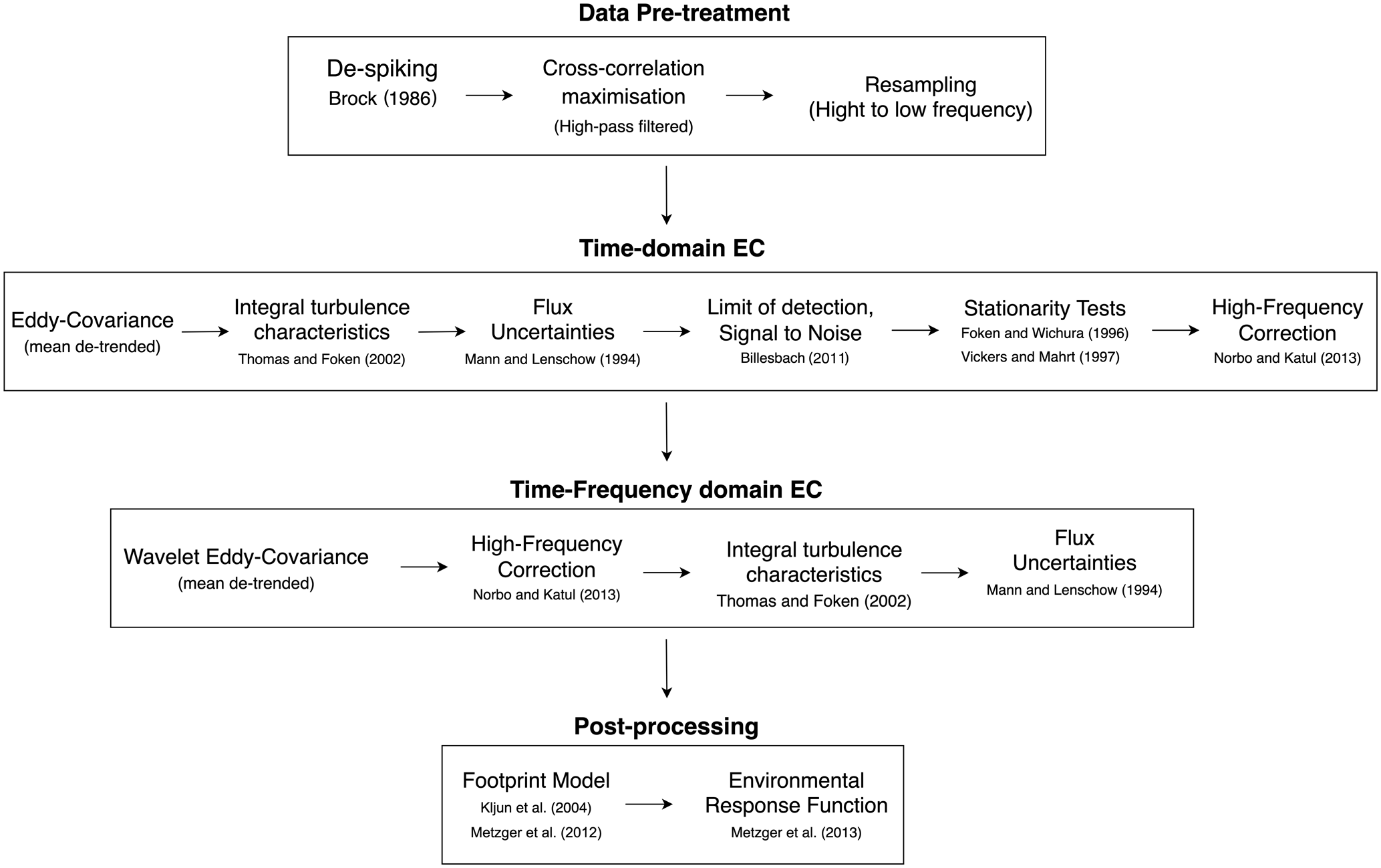
Figure 2 Modular eddy4R workflow giving four processing steps: raw data pre-treatment, time-domain EC, time-frequency-domain EC, and post-processing analysis (footprint and ERF).

The eddy4R flux processing followed the workflow shown in Fig. 2. Individual transects were processed separately, with a minimum flight distance of 15 km, ensuring large atmospheric transport scales were captured. Data periods containing sharp turns or orbital loops were omitted. Meteorology, position and concentration data were merged for each transect, giving a regularised data frame at 20 Hz. Each transect was screened for data outside of defined thresholds and omitted. The overall data pass rate was set to ≥ 90 %. Successful transects underwent de-spiking using the method outlined by Brock (1986) in the form of Starkenburg et al. (2016) for wind vectors ($u,v,w$), temperature and NO and NO₂ mixing ratios. The technique is sensitive to up to four consecutive data spikes. High-pass filtered cross-covariance maximisation (Hartmann et al., 2018) was applied to correct NO $/$ NO₂ mixing ratios and air temperature for differences in sampling time compared to the vertical wind (w). Once lag-time corrected, data were resampled from 20 to 9 Hz using mean rolling averaging (Zeileis and Grothendieck, 2005).

Table 2 List of eddy-covariance parameters for quantifying airborne NO_x fluxes.

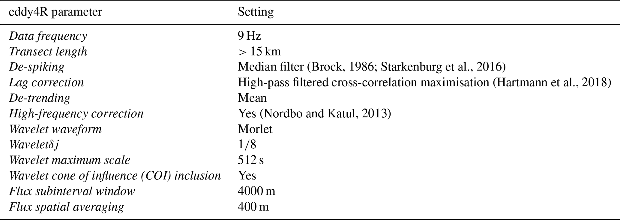
After data pre-treatment, time-domain (classical) and time-frequency-domain (wavelet) fluxes were calculated as outlined in Fig. 2. Time-domain EC gives a single flux estimate per transect, whereas time-frequency EC gives a flux measurement every 400 m along the transect using an overlapping 4000 m moving window. Time-frequency EC uses CWT for flux analyses. A minimum wavelet scale of 4.5 Hz (Nyquist frequency) and a maximum scale of 512 s were chosen for the wavelet calculations; 512 s was chosen to ensure all long-scale transport processes were accounted for, as shown in Fig. S4, whereby scales above this point do not show significant emission structure. Wavelet cone of influence was not removed in accordance with Metzger et al. (2013). Table 2 outlines eddy4R processing parameters.

Each flight leg underwent the following QA/QC steps. Each flight transect was screened for the presence of clear cross-covariance peaks for NO, NO₂ and temperature (Fig. S3). Limit of detection (LOD) (Billesbach, 2011) and signal-to-noise (S $/$ N) statistics (Foken and Wichura, 1996; Vickers and Mahrt, 1997) were calculated and median flux LODs were found to be 0.19 mg m⁻² h⁻¹ for NO and 0.57 mg m⁻² h⁻¹ for NO₂. Fluxes below these thresholds were flagged. Median S $/$ N statistics for NO and NO₂ fluxes were found to be 14.54 and 17.26. Stationarity tests were calculated for each flight transect, with a flag threshold of 100 % used (Foken and Wichura, 1996; Vickers and Mahrt, 1997). Nine out of 42 transects failed the stationarity criteria and so were omitted. NO and NO₂ fluxes were assessed for high-frequency spectral loss using a wavelet-based correction methodology (Nordbo and Katul, 2013). Average high-frequency loss factors for NO and NO₂ were found to be 1.014 and 1.015. As these corrections increased fluxes by only 1.4 %–1.5 %, they were not applied. A detailed overview of chemical and meteorological NO_x flux losses can be found in Vaughan et al. (2016). As a final QA/QC filter, friction velocity (u*) was chosen as a metric of developed turbulence. A u* threshold of 0.15 m s⁻¹ was chosen in line with other urban EC studies (Langford et al., 2010; Squires et al., 2020), with data falling below this value being filtered out.

2.3.2 Footprint model

To assess the spatial influence of each flux, we used a footprint model. The model calculates a spatial representative weighting matrix for each measurement along the flight track. In this study, we apply a model capable of assessing influence from prevailing wind and crosswind (Metzger et al., 2012). The model uses a parameterised version of the Kljun (KL04) backwards Lagrangian model (Kljun et al., 2002, 2004), capable of calculating footprint estimates under stable and strongly convective conditions. Parameterisation was achieved using measurement height (Z_m), u*, standard deviations of vertical and horizontal wind speeds, the planetary boundary layer height (Z_i) and aerodynamic roughness length (Z₀). We used previously published Z₀ values for the GLR, accounting for westerly and easterly wind influences, at 1 km² resolution (Drew et al., 2013). The model generates a weighting matrix across the same domain as the spatial dataset of interest, summing up to 1, and is centred on the aircraft's location. The footprint matrix can then be used to weight and cumulatively sum the spatial dataset, giving a representative value along the flight leg. Figure 3 shows the average calculated footprint across the campaign at 30 %, 60 %, and 90 % influence contours. On average, the 90 % influence distance ranged from 3 to 12 km.

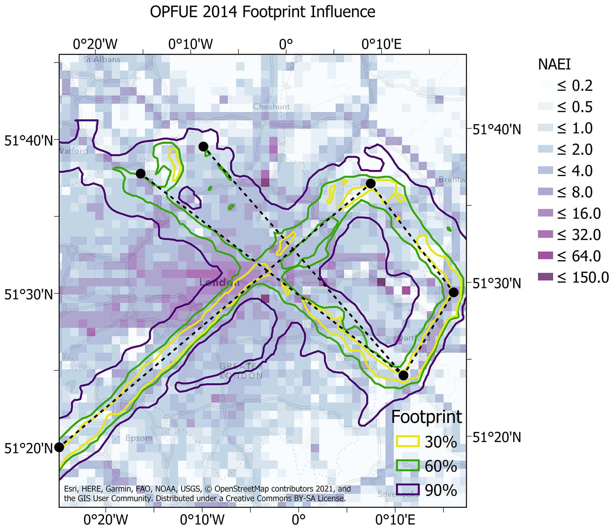
Figure 3 Footprint climatology of all aircraft transects, indicated by the 30 %, 60 % and 90 % contour lines of the cumulative surface influence superimposed over the 2014 NAEI for NO_x emissions in tons km⁻² yr⁻¹. Plotted in ArcGIS^® (Esri, 2021b).

2.3.3 Boosted regression tree machine learning

Linking time-of-day measured fluxes at the aircraft transect height to the surface can be challenging and is driven mainly by their spatio-temporal variability. The application of an ERF, in contrast, can bridge this gap by building relationships between measured flux (spatial and temporal) and environmental drivers. We used boosted regression trees (BRTs) (Elith et al., 2008; Metzger et al., 2013; Serafimovich et al., 2018) to calculate ERF relationships between measured airborne fluxes (spatial and temporal) and multiple environmental drivers. BRT is a non-parametric machine learning technique that combines regression trees and boosting to formulate ERF relationships (Serafimovich et al., 2018). BRT parameters were determined using the same strategy as Metzger et al. (2013) through the cross-validation procedure described in Elith et al. (2008). We found by using a learning rate of 0.1, tree complexity of 6, bag fraction of 0.75, absolute (Laplace) error structure and 3.7 × 10⁴ trees overall that we were able to minimise the predicted deviance whilst achieving the optimum model fit. The BRT approach used an initial 500 trees, with 500 trees added at each step. The training dataset consisted of 1751 airborne flux observations after QA/QC filtering.

3 Results and discussion

3.1 Airborne NO_x fluxes

NO_x fluxes were calculated during four flights, giving 11 complete transects across the GLR and 2884 individual 400 m flux averages. Measurements were made at a relatively constant altitude above the surface (340 ± 40 m), corrected for both terrain elevation and building height. Building height data for the entire Greater London region were obtained from the Digimap Ordnance Survey Web Map Service (Digimap) (Ordnance Survey, 2020). To account for changing boundary layer heights, we used hourly 0.25^∘ estimates from the ERA5 fifth-generation ECMWF reanalysis for global climate data (Hersbach et al., 2018). The calculated depth of the boundary layer ($Z_{\mathrm{m}}/Z_i$) ranged from 0.150 to 0.770, with a median $Z_{\mathrm{m}}/Z_i$ of 0.255. Atmospheric stratification was found to be mostly unstable throughout the campaign, with a median Obukhov length (L) of −182 m and a dimensionless Monin–Obukhov stability parameter ($Z_{\mathrm{m}}/L$) of −1.98. Friction velocities ranged from 0.06 to 1.09 m s⁻¹, with an average of 0.56 m s⁻¹.

EC measurements are affected by random and systematic uncertainties. Random error accounts for uncertainty due to an insufficient averaging period, resulting in the inadequate sampling of primary contributing eddies (Lenschow et al., 1994; Mann and Lenschow, 1994). A detailed review of random error estimation approaches for EC can be found in Salesky et al. (2012). Systematic error accounts for undersampling of the largest atmospheric scales responsible for turbulent flux (Lenschow et al., 1994; Mann and Lenschow, 1994). At a 400 m averaging interval, the median random error (± median absolute deviation) for the NO flux was 126.6 ± 80.6 % and 108.3 ± 58.5 % for NO₂. The median systematic errors for NO and NO₂ flux were 14.7 ± 4.7 % and 14.3 ± 4.5 %. Chemical loss of NO_x to OH was not corrected for in this study, which is in line with the discussion in Vaughan et al. (2016), with such losses being small (1 %–2 %).

As the Fast-AQD-NO_x quantifies mixing ratios of NO_x in wet air, the effect of density fluctuations (WPL) on calculated NO_x flux was assessed using the method described by Hartmann et al. (2018, Eq. 21). Fast (20 Hz) mixing ratios of water vapour were calculated from relative humidity, pressure, and temperature data and corrected for lag-time differences to the vertical wind. The water vapour mixing ratio was used to convert NO $/$ NO₂ mixing ratios to dry mole before performing EC calculations. Figure S6a shows the linear regression between uncorrected and corrected NO_x flux for the influence of WPL. Correcting for WPL increased measured NO_x flux on average by 1.35 %. In addition to WPL corrections, the effect of vertical flux divergence was also investigated. Vertical divergence can account for significant flux losses due to weakening vertical momentum at increased altitudes below the planetary boundary layer (Deardorff, 1974; Sorbjan, 2006). Figure S6b shows corrected vs. uncorrected NO_x flux using the method outlined by Sorbjan (2006), showing a potential 50 % flux increase. Due to the coarseness of the ERA5 PLB data at 0.25^∘ resolution and the complexity of London's surface structure, a more detailed assessment is needed to understand what potential effects vertical flux divergence may have on urban emission estimates. Due to strict air traffic control restrictions, vertical profiles were not possible during the campaign, which would have allowed for a more detailed assessment of divergence influences. The NO_x fluxes reported in this study are not corrected for vertical flux divergence and so will be considered conservative due to the listed processes having the potential to further increase measured rates.

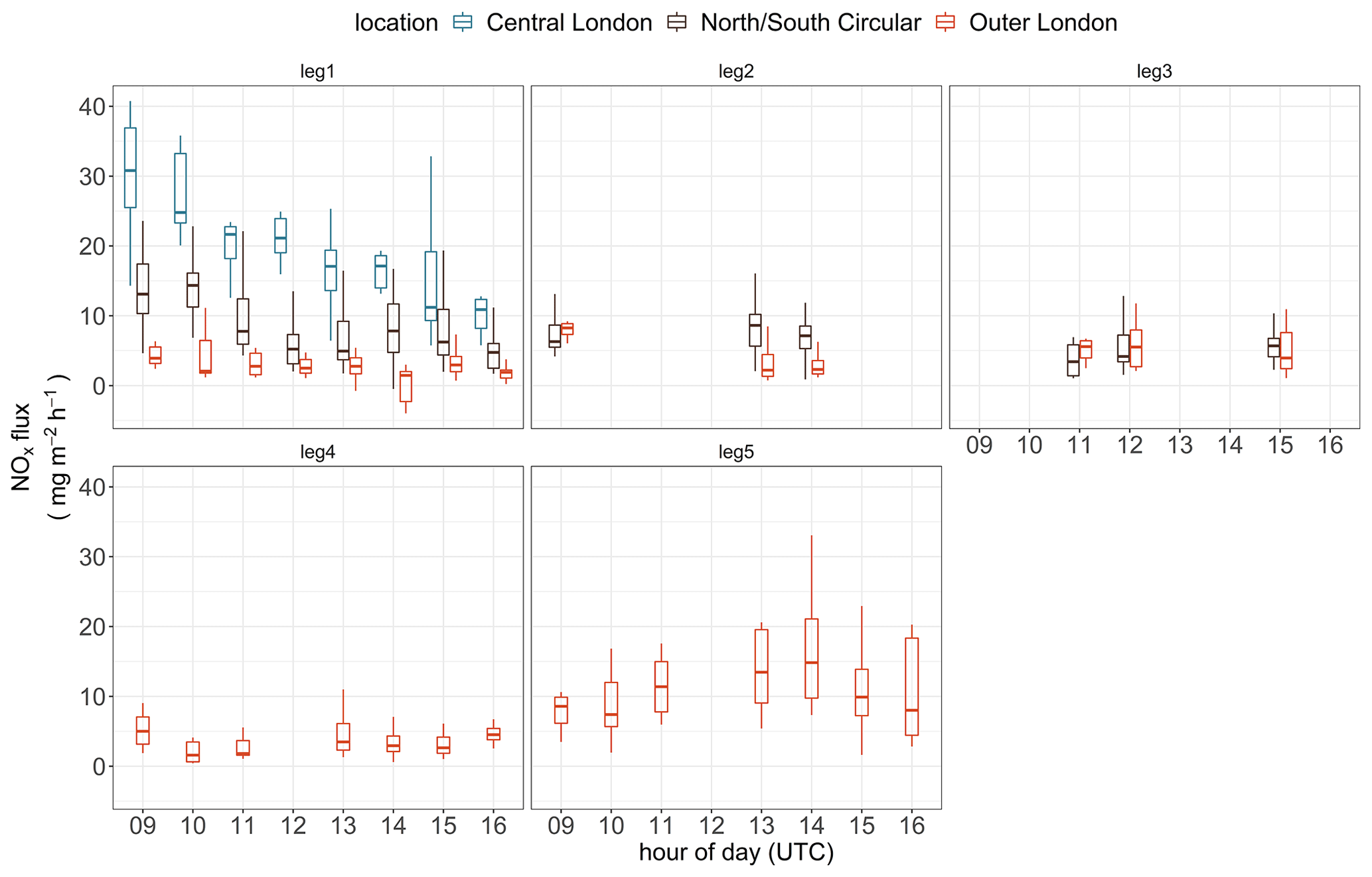
Figure 4 Hourly boxplot analysis of measured NO_x fluxes, grouped by flight leg type and location within London. Groupings have been defined as the following. Central London (51.48–51.52^∘ N, 0.17–0.07^∘ W). North/South Circular (51.44–51.6^∘ N, 0.29^∘ W–0.07^∘ E), excluding the Central London area within. Outer London (51.25–51.7^∘ N, 0.54^∘ W–0.29^∘ E), excluding both the Central London and North/South Circular areas within.

Flux measurements were made across a 5 d period, giving three weekdays (Monday–Wednesday) and one weekend day (Saturday). The temporal distribution of measurements is well distributed, ranging from 08:00 to 16:00 UTC. Hourly averaging across the entire dataset shows a partial diurnal profile, with the maximum hourly mean NO_x flux for the GLR occurring at 10:00 UTC (8.95 mg m⁻² h⁻¹). The diurnal profile does not extend past 16:00 UTC, due to encountered air traffic control time restrictions. The present diurnal is complex due to limited flight hours and the spatial variation of measured fluxes. Focus on the temporal component: fluxes were hourly bin averaged and grouped according to the flight leg type (Fig. 1) and measurement location with three defined areas: Central London, the North/South Circular area and Outer London. Figure 4 shows hourly boxplot flux averages for each flight leg type vs. location in London. Leg 1 showed a strong morning diurnal for the Central and North/South Circular areas of London, compared to legs 2 and 3, which typically showed consistent NO_x emission rates across the different hours sampled. Emissions measured during the hours of 08:00-10:00 UTC in Central London are above 20 mg m⁻² h⁻¹, which is consistent with other London studies assessing London emissions (Lee et al., 2015). The temporal variability of leg 5 was contrastingly different to the other four legs and is heavily influenced by road transport emissions (M25 orbital motorway).

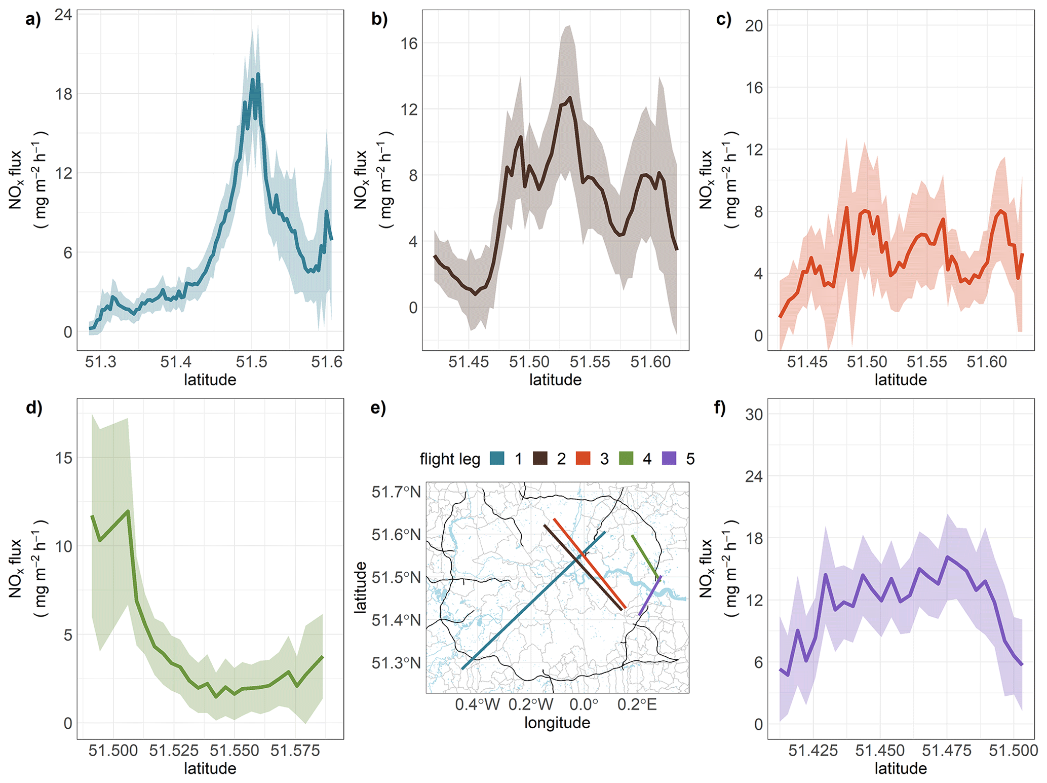
Figure 5 Ensemble NO_x flux flight track averages (400 m) across the campaign, with the shaded area representing the average random error divided by the square root of the number of sample points which went into each mean (error $/$ $\sqrt{n}$). The top row (a, b c) shows flight transects 1, 2 and 3, which ran over central areas of London such as the City of London borough. The bottom row (d, f) transects 4 and 5 ran over eastern regions of Greater London, home to industry and a major road network. Panel (e) shows each individual track transect overlaid onto OpenStreetMap's; major road infrastructure, local boundaries, and rivers around the GLR (© OpenStreetMap contributors, 2021. Distributed under the Open Data Commons Open Database License (ODbL) v1.0.; Padgham et al., 2020).

By aggregating and averaging across multiple transects, the temporal variability can be better accounted for, giving a clearer picture of the spatial component. Figure 5 shows mean 400 m latitude flux averages for each of the five transect types. The shaded area shows the average flux random error divided by the square root of the number of sample points which went into each mean. Averaging reduces the individual flux uncertainty (> 100 %), with the average flux uncertainty (average error $/$ $\sqrt{n}$) being 48.7 ± 20.7 %. Transect 1 follows an identical path to that of similar measurements made previously in 2013 and shows comparable NO_x fluxes (Vaughan et al., 2016). The highest observed fluxes (> 20 mg m⁻² h⁻¹) were measured over the London borough of Southwark and the City of London. Both areas include major roads, national rail stations and densely packed high-rise buildings, giving profoundly heterogeneous emissions sources of NO_x. Transects 2 and 3 (Fig. 5) ran perpendicularly to transect 1, giving emission information over the south-eastern and north-western areas of Greater London. The emission structure of transect 2 shows similarities to that of transect 1, with fluxes in the central area above 10 mg m⁻² h⁻¹. Transect 3, in comparison, showed 50 % lower emissions (5 mg m⁻² h⁻¹). This transect was over more suburban areas compared to transects 1 and 2. The final transects (4 and 5) ran over eastern parts of the GLR, extending out to the M25 orbital motorway and industrial infrastructure. The Dartford Crossing (A282) area showed elevated NO_x emissions (> 10 mg m⁻² h⁻¹). It was evident during most flights that this area was prone to congestion, suggesting vehicles as the primary source. The design capacity of the bridge is 135 000 vehicles d⁻¹, but vehicle flows now routinely exceed 160 000 d⁻¹.

3.2 Comparison to the emission inventory

Measured fluxes are a powerful tool for evaluating bottom-up emission estimates, such as the NAEI. The NAEI is vital for assessing UK air quality, providing annual emissions estimates for a range of pollutants at 1 km² resolution for the UK region. Each pollutant has an individual bottom-up inventory, covering hundreds of different emissions categories, which, when summed together, give an annual national estimate. These sources include road transport, domestic and industrial combustion, rail, aviation, energy generation, waste, fossil fuel extraction and agricultural production. The NAEI's road transport sector is based on UK road traffic statistics and the COPERT (Calculation of Emissions from Road Transport) 4 emission factor model, which is part of the European Monitoring and Evaluation Programme/European Economic Area (EMEP/EEA) air pollutant emission inventory guidebook (Bush et al., 2008; EEA, 2013). For each airborne flux, a footprint matrix was generated at the same spatial extent and resolution (1 km²) as the NAEI, using the described footprint model. Each footprint equates to a value of 1 and weights each grid cell of the NAEI individually. Once weighted, all cells are summarised, giving a spatially representative emission estimate. We corrected for time-of-day emission variations by scaling each source sector individually for monthly, daily and hourly influences using factors unique to each sector. Once scaled, all sources are summed to produce a time-of-day estimate, comparable to the location and time-of-day each flux measurement was made.

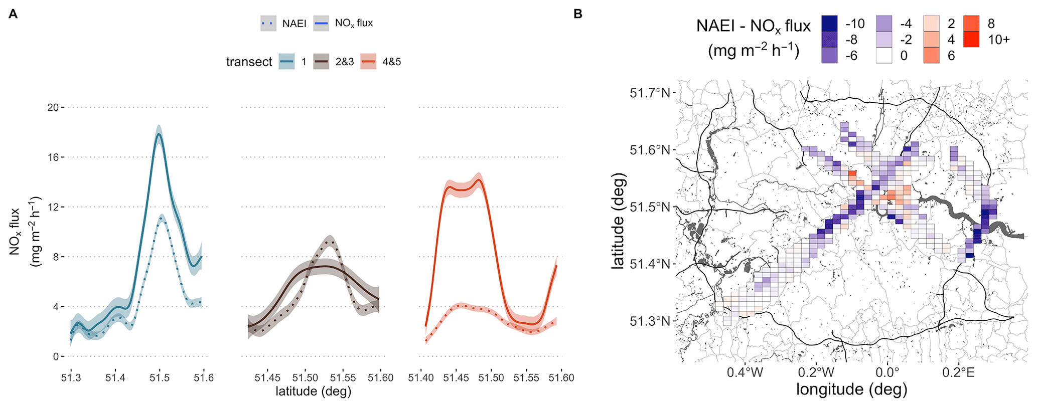
Figure 6 (a) Transect-grouped NO_x flux and NAEI emission estimates as a function of latitude. A generalised additive model (GAM) has been fitted to each transect grouping using a k value of 10. The 95 % confidence interval of the GAM is shown as the light shaded area. (b) Spatially median binned 1 km² difference between predicted NO_x emissions (NAEI) and measured NO_x fluxes, mapped onto OpenStreetMap's; major road infrastructure, local boundaries, and rivers around the GLR (© OpenStreetMap contributors, 2021. Distributed under the Open Data Commons Open Database License (ODbL) v1.0.; Padgham et al., 2020).

Table 3 Predicted NAEI emissions sources grouped by transect time and the median ratio of measurement to NAEI estimate (± median absolute deviation). These sources are road transport, other transport such as rail and shipping, domestic combustion (combustion in commercial, institutional, residential and agriculture), industrial combustion (combustion in industry) and energy production (combustion in energy production and transformation).

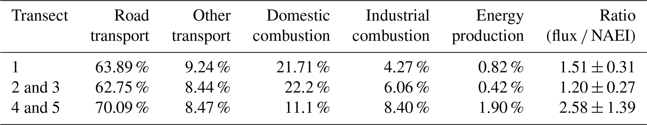
To compare measured fluxes against footprint-calculated time-of-day NAEI estimates, each transect type was 1 km mean binned as a function of latitude. Transects 2 and 3 were grouped to produce a perpendicular comparison to transect 1. Transects 4 and 5 were grouped to give a comparison in an area more representative of industrial/road transport-dominated emissions sources. Figure 6a shows the measured flux (solid) and time-of-day scales' NAEI estimates (dotted) as a function of latitude for each of the three groupings using a generalised additive model (GAM) fit (Hastie and Tibshirani, 1990). The GAM fits a non-linear distribution to the data, being either the measured flux or time-of-day inventory estimate as a function of latitude. The shaded area shows the 95 % confidence interval of the GAM fit. Measured fluxes along transect 1 consistently showed higher NO_x emissions than estimated by the NAEI (mean of 1.5 times higher). The greatest divergence ratio between the measured and inventory-estimate fluxes was 1.98, which is broadly consistent with previous studies (Lee et al., 2015). The divergence for transect 1 was most substantial when a mix of different emissions sources were encountered, such as other transport mediums (rail and shipping) and domestic and industrial combustion settings (see Table 3). Comparison for grouped transects 2 and 3 showed improved agreement with the inventory, with measured fluxes on average 1.21 times higher. The percentage contribution of emissions sources was similar to transect 1, with only a slightly lower average road transport contribution (63 %). The stronger agreement between transects 2 and 3 suggests the high emissions observed during transect 1 are dependent on either a missing or under-represented source in the inventory. Grouped transects 4 and 5 also displayed a high degree of divergence from the inventory. On average, the ratio between measurement and inventory was 2.57, with a peak value of 4.45. The primary sources for this area include a greater contribution from energy production and industrial combustion. Table 3 summarises the three different groups, with average NAEI sector contributions and the ratio between flux measurement and inventory.

Spatially, the disagreement between measurement and inventory is uneven, as shown by Fig. 6b, whether, for each 1 km along the flight track, the median inventory minus measurement value has been calculated. South-western areas of the GLR agree better than the central and north-eastern areas. Greater underestimation by the inventory compared with measurements was predominantly observed in regions of complex source distribution and where no single primary source dominated. The extent of disagreement highlights the challenges and consequent drawbacks of using the NAEI as a predictive tool for estimating NO_x emissions or as a time-of-day diagnostic for measured NO_x fluxes. Several vital processes may likely contribute to the observed differences, in addition to NO_x emissions being higher than in the NAEI. The first is inventory scaling from annual to time-of-day. As each source sector undergoes individual scaling, these factors play a significant role in predicting time-of-day influences. Currently, these factors lack spatial disaggregation and do not account for the unique temporal profiles present per area. In contrast to the NAEI, the London Atmospheric Emissions Inventory (LAEI) uses emissions data from individual vehicle classes, obtained by on-the-road `remote sensing', to constrain its predicted emissions from the road transport sector, giving a more realistic comparison to “real-life” emissions and hence to eddy-covariance measurements (Lee et al., 2015; Vaughan et al., 2016).

3.3 Spatio-temporal emissions

To overcome the limitation of using time-of-day representative NAEI estimates to explain measured fluxes, a more pragmatic approach was chosen. Using the outlined ERF methodology, we attempted to generate representative emission grids for each flight transect. To train the BRT technique, NO_x flux data were filtered to include 0.5 % to 99.5 % quantile values and positive fluxes only. We found excellent agreement between measured and ERF-reproduced NO_x fluxes in the range of 0–37 mg m⁻² h⁻¹. The two datasets agreed close to a 1 : 1 trend (0.96), with an R² coefficient of correlation of > 0.99 and a residual standard deviation of 0.01. Figure S7a shows the linear regression between median-averaged measured flux vs. BRT model prediction for each flight transect.

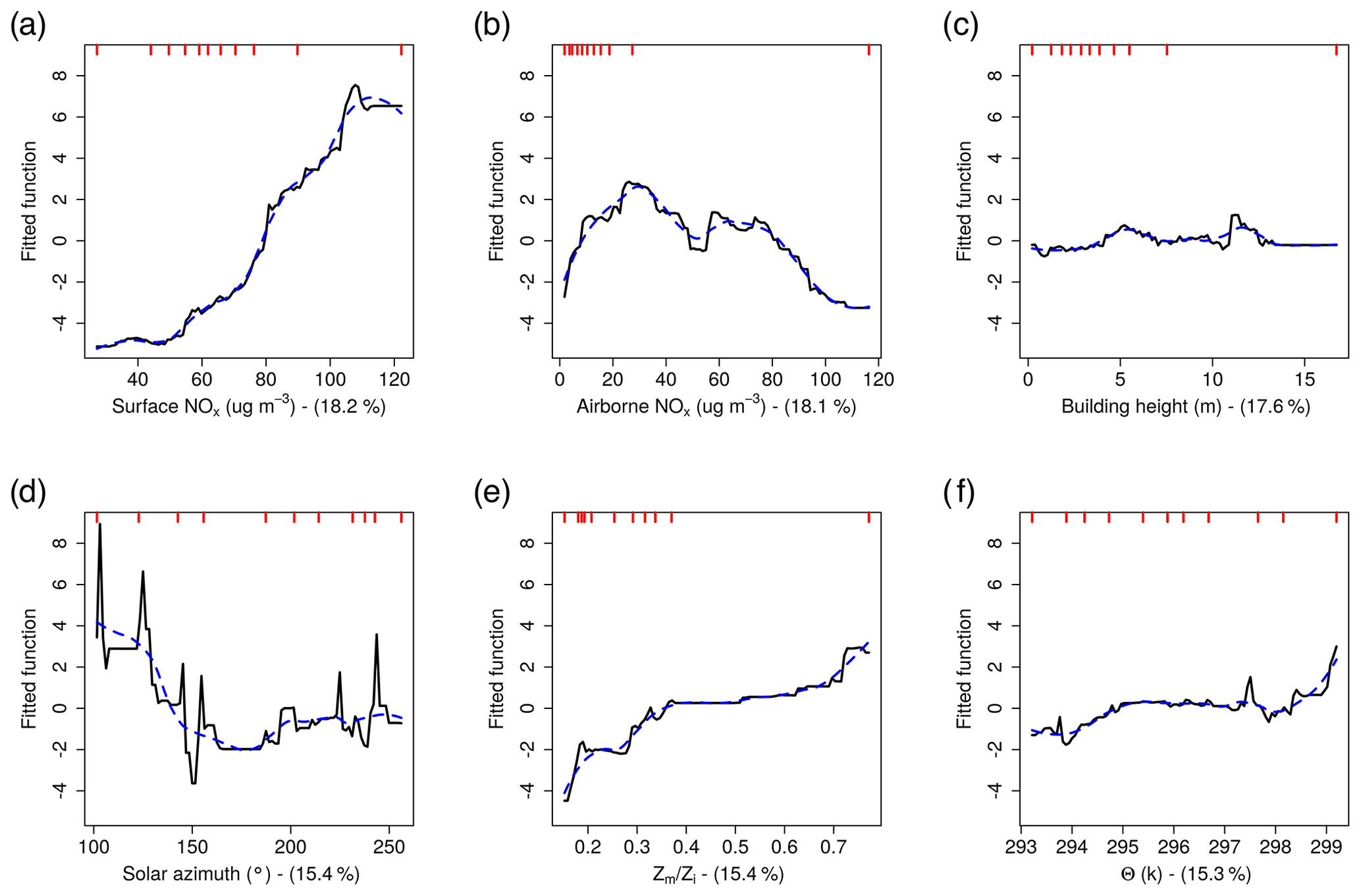
Figure 7 Partial dependency plots for six environmental drivers, showing BRT-fitted ERFs (black line) for each driver as a function of flux dependency from the mean, ranked in terms of percentage contribution (%) towards accounting for NO_x flux distribution. The red degree marks on the top x axis show the data distribution from 0 % to 100 % in 10 % bins. The blue line shows the smoothed trend for each dependency plot.

Six environmental drivers were used in the ERF process to describe the spatio-temporal nature of the measured NO_x fluxes. Figure 7 shows the partial response functions calculated for each driver against difference from the mean flux and ranked in terms of percentage contribution to the flux distribution. Two different spatial datasets were used to account for the complex heterogeneity of the Greater London region (Fig. 7a and c). Using the described footprint methodology, spatially representative surface NO_x concentrations and building heights were calculated for each flux from the LAEI and Ordnance Survey datasets (Greater London Authority, 2013; Ordnance Survey, 2020). Preliminary analyses using surface NO_x concentration as the only spatial driver appeared to overweight suburban areas and underweight central areas of the GLR. The combination of the two datasets helps to reinforce the significant spatial differences between outer and inner London. To account for meteorological differences, NO_x concentration at altitude (Fig. 7b), relative measurement height in the boundary layer ($Z_{\mathrm{m}}/Z_i$) and potential temperature were chosen as ERF drivers (Fig. 7e and f). As shown in Fig. 7e, 90 % of flight data occur below a $Z_{\mathrm{m}}/Z_i$ value of 0.4, with the function above 0.4 being mainly linear. Solar azimuth angle (Fig. 7d) was chosen to account for temporal variations in the measured flux. Flight data are well distributed across the solar azimuth angle domain from 100 to 260^o, corresponding to 08:00–16:00 UTC.

Figure 8 The median average projection of NO_x emissions (mg m⁻² h⁻¹) at 400 m² resolution from all flight transect data. The standard deviation (b) and relative standard deviation (c) show the variability between individual flight transect projects. Missing areas outside of the ERF training dataset are shown in grey.

For each flight leg, surface-layer NO_x fluxes were projected using median calculated statistics. Median values were chosen to account for the high heterogeneity across the length of a flight leg. $Z_{\mathrm{m}}/Z_i$ values for each ERF flux projection were kept constant to enable comparison between legs. Overall, 20 unique transects were projected onto an aggregated 400 m² LAEI grid, marrying to the spatial resolution of measured flux. Figure 8 shows the median average of all ERF flux projections across the field campaign. Overall, ERF flux projection was possible across 98 % of the GLR domain. Strong NO_x emission rates are exhibited in Central London, with lower emissions in Outer London. The standard deviation between individual flight transects is low, showing ±2.45 mg m⁻² h⁻¹. The calculated relative standard deviation (RSD) shows a more complex picture, with predicted emissions in outer regions of London having a high RSD (> 40 %) compared to Central London (> 35 %). Figure 8c shows the calculated RSD across the GLR domain, suggesting central areas showed a more consistent emission profile during the campaign, highlighting the need for further refinement of how the ERF predicted emissions in outer areas of London. ERF did not extrapolate onto areas of much higher or lower surface NO_x concentrations (shown as grey), which exceeded the ranges observed in the training dataset. These areas included parts of the M25 orbital motorway due to limited data airborne over the region and where footprints extended beyond the confines of the LAEI grid. Areas of Central London are also left blank due to footprints not encountering surface concentrations above 122 µg m⁻³.

To assess the performance of the BRT model, one flight transect was omitted at a time, and the incomplete model was then used to predict the omitted dataset. Figure S7b shows the comparison between the predicted median flight emission average using the incomplete model vs. the complete one. Linear regression gives a slope of 0.867, with the incomplete model, on average, overpredicting fluxes by 13.8 % (0.74 mg m⁻² h⁻¹), which is taken as the prediction uncertainty of the complete BRT model. The difference between the two models is comparable to the finding of Metzger et al. (2013), which found model differences for sensible and latent heat flux to be between 11 % and 18 % using the same technique. The spatial uncertainty distribution across the GLR is complex, as shown in Fig. S7c. The incomplete model generally overestimates NO_x emissions in Outer London more significantly than in Central London, where the models align more strongly. The prediction performance of the BRT model varied from flight transect to transect, as shown in Fig. S8. The majority of flight leg projects successfully scaled Central London emissions comparably to that of measured fluxes. The projects also successfully captured key features in the flux observation, such as major road networks and densely populated areas.

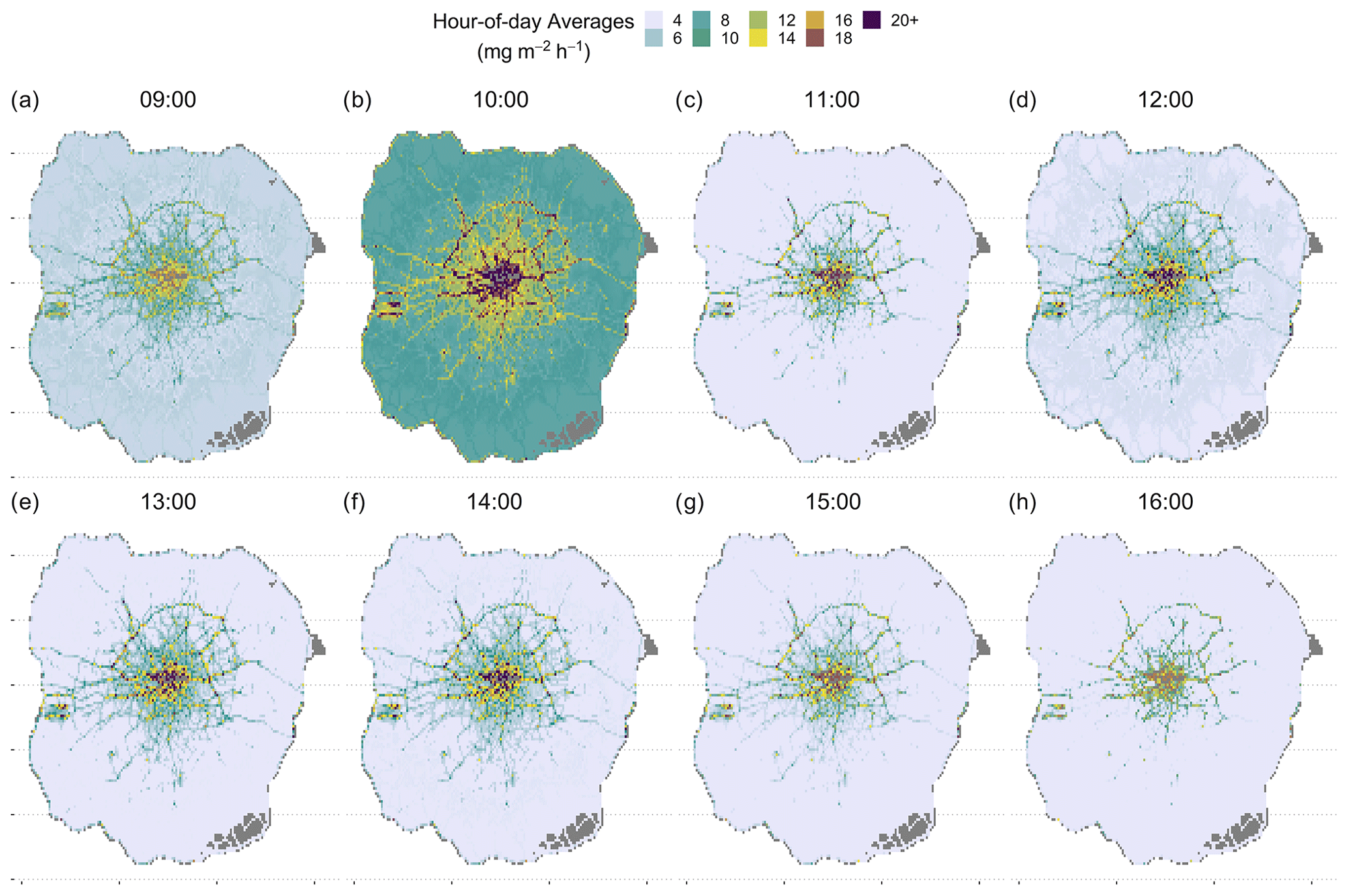
Figure 9 Hour-of-day ERF flux projections from 09:00 to 16:00 UTC. Grey colour highlights areas outside of the ERF training dataset. The strong presence of the morning rush-hour period is observed from 09:00 to 10:00 UTC (a–b).

The diurnal variability was also investigated during the campaign by grouping flight data into hourly bins and using the median hourly statistics to drive each ERF flux projection. Again, $Z_{\mathrm{m}}/Z_i$ was kept constant for all projections. Figure 9 shows the average hourly ERF projections, spanning an 8 h period from 09:00 to 16:00 UTC. All projections retain a strong heterogeneous profile. The most substantial emission rates were observed during 09:00–10:00 UTC (Fig. 9a–b), aligning with the morning rush hour. The emission rates rise across the GLR, in unison, until 10:00 UTC, when emissions stabilise into the afternoon period. Projected Central London emissions during this period agree well with measured fluxes, whilst more suburban areas are potentially scaled too high, suggesting further temporal refinement across the domain is required. The evening rush hour, previously observed in NO_x emissions in London after 16:00 UTC (Lee et al., 2015), is not captured in these predictions.

4 Conclusions

The assessment of NO_x emissions in urban areas remains an important area for research due to the critical impacts that high NO_x concentrations have on local public health and the attainment of national transboundary emissions commitments. In this study, we used airborne measurements over the Greater London area to upscale airborne NO_x flux observations to high-resolution emission projections across the region via environmental response function (ERF) physics-guided flux data fusion. The work presented here presents a method which can quantify and spatially disaggregate NO_x fluxes over challenging urban terrain and has the potential to be applied to other metropolitan areas worldwide.

Seven low-altitude research flights were made over the Greater London region (GLR) in July 2014, performing multiple overpasses across the city. From these flights, 2715 individual NO_x fluxes at 400 m spatial resolution were measured and processed in R using the eddy4R software. Measured NO_x fluxes across the Greater London region exhibited high heterogeneity and substantial diurnal variability. Central areas of London showed the highest emission rates quantified during the campaign. Other high-emission source areas included the M25 orbital motorway. The complexity of London's emission characteristics makes it challenging to pinpoint single emissions sources definitively. In practice, multiple sources are likely to contribute to measured fluxes at the spatial scale used here, including road transport and residential, commercial and industrial combustion (mainly for space heating). To give a time-of-day reference, we compared measured fluxes to the UK's National Atmospheric Emissions Inventory, scaled to account for monthly, daily and hourly differences from the annual values. We found that for central areas of London, the inventory underestimated emissions by up to a factor of 2, which is consistent with other published studies. Measured fluxes were consistently higher than inventory estimates across most of Greater London.

To overcome the limitations of comparing to the national inventory, we trained ERFs between measured spatial–temporal NO_x fluxes and environmental drivers (meteorological and surface) to generate time-of-day emission surfaces. ERF successfully reproduced aircraft-measured NO_x fluxes, with a coefficient of determination (R²) of 0.99. We used the calculated ERF relationships to project the NO_x flux for the time of each flight transect across the GLR domain at 400 m² resolution. We were able to achieve a 98 % spatial coverage and a highly heterogeneous emission surface. The overall variability between ERF flux projections was low, with an average relative standard deviation of 40 %. All ERF flux projections showed high emissions emanating from central areas of London and the major road network. Hour of day projections highlighted a strong morning rush hour, peaking at 10:00 UTC and remaining elevated into the afternoon. Overall, the integration of high-resolution spatio-temporal fluxes with an ERF-driven strategy has enabled the generation of spatial NO_x emissions at high resolution over Greater London.

This work demonstrates the power of airborne eddy-covariance-based measurements of air pollutant fluxes as a tool for evaluating emission inventories or as a method of independently obtaining spatially disaggregated city-wide emission rates of pollutants. The method is applicable to other metropolitan areas or any other heterogeneous landscape. It should also help legislating authorities better understand air pollution sources and the effectiveness of control measures.