the Creative Commons Attribution 4.0 License.
the Creative Commons Attribution 4.0 License.
 | 13 Oct 2021
Aerosol–cloud interactions: the representation of heterogeneous ice activation in cloud models
Claudia Marcolli
The homogeneous nucleation of ice in supercooled liquid-water clouds is characterized by time-dependent freezing rates. By contrast, water phase transitions induced heterogeneously by ice-nucleating particles (INPs) are described by time-independent ice-active fractions depending on ice supersaturation (s). Laboratory studies report ice-active particle number fractions (AFs) that are cumulative in s. Cloud models budget INP and ice crystal numbers to conserve total particle number during water phase transitions. Here, we show that ice formation from INPs with time-independent nucleation behavior is overpredicted when models budget particle numbers and at the same time derive ice crystal numbers from s-cumulative AFs. This causes a bias towards heterogeneous ice formation in situations where INPs compete with homogeneous droplet freezing during cloud formation. We resolve this issue by introducing differential AFs, thereby moving us one step closer to more robust simulations of aerosol–cloud interactions.
- Article
(909 KB) - Full-text XML
- BibTeX
- EndNote


A wide variety of macromolecular or proteinaceous, crystalline, glassy, and solid aerosol particles act as INPs in the atmosphere and participate in the formation of cirrus or in the glaciation of supercooled liquid-water clouds (Kanji et al., 2017). Among the various modes of heterogeneous ice formation, immersion freezing caused by INPs present within a volume of supercooled liquid water is considered the most relevant mode in mixed-phase clouds (Vali et al., 2015). Alternative freezing modes include contact freezing, where ice forms upon the collision of an INP with a cloud droplet, and condensation freezing, where ice nucleates while the cloud forms through cloud droplet activation. In conditions below liquid-water saturation, deposition nucleation occurring in the absence of liquid water has traditionally been considered the most relevant heterogeneous ice formation mode (Vali et al., 2015). Yet, there is increasing evidence that the loci for ice nucleation on INP surfaces are pores in which water gathers below water saturation through capillary condensation (Marcolli, 2014; Kiselev et al., 2017; Holden et al., 2019). Pore condensation and freezing (PCF) involves homogeneous ice nucleation within pores under cirrus conditions (air temperature T<233 K) and may occur heterogeneously through immersion freezing in mixed-phase clouds at higher temperatures (David et al., 2019; Marcolli, 2020).
In laboratory experiments, phase transitions from supercooled liquid water to ice are observed under controlled temperature and relative humidity conditions during set observational times for ice detection (Cziczo et al., 2017). In experiments employing droplet freezing techniques, ice nucleation is detected in arrays of droplets deposited on a substrate. Results are normalized based on total droplet number, surface area, or volume to obtain freezing spectra that are usually reported in terms of cumulative ice-active fractions (Vali, 2019). Laboratory experiments using cloud or continuous-flow chambers directly provide number fractions, ϕ, of ice-activated or frozen particles from a sample of size N0 as a function of ice supersaturation, s. These fractions vary between 0 at s=0 (ice saturation) and 1 at sufficiently large s and are cumulative, reflecting measurements in which the ice nucleation ability of a given sample is probed at successively increasing s values. The total number of ice crystals formed up to a value of s is then determined via N0ϕ(s). In the case of immersion freezing experiments, where an ensemble of water droplets with immersed INPs is cooled, frozen fractions are parameterized as a function of supercooling (temperature, T) instead of supersaturation such that differential and cumulative AFs are functions of T instead of s.
During immersion freezing, ice nucleates over a wider temperature range compared with homogeneous freezing of pure water droplets (Peckhaus et al., 2016; Tarn et al., 2018). Heterogeneous freezing curves become even broader when a mixture of different INP types is investigated. Yet, when one and the same droplet is repeatedly probed in freezing–thawing cycles during refreeze experiments, freezing occurs in a temperature range that is similarly narrow to that for homogeneous freezing (Kaufmann et al., 2017).
While the broad range of freezing temperatures observed for an ensemble of droplets with immersed INPs can be ascribed to the deterministic (time-independent) component of freezing given by the characteristic freezing temperature of nucleation sites, the much narrower spread of freezing temperatures observed in refreeze experiments evidences the stochastic (time-dependent) component on specific nucleation sites. Therefore, purely deterministic formulations correctly encompass the broad variability of nucleation sites evidenced in the freezing of particle/droplet ensembles, while neglecting the variability due to stochastic nucleation on specific sites evidenced in refreeze experiments. Thus, applying a deterministic description of immersion freezing in cloud models is justified, as the stochastic component just induces a minor modulation of the characteristic freezing temperatures.
PCF is described by a deterministic parameterization as well, as ice formation in this mode is determined by the relative humidities required either for pore water condensation or ice growth with no stochastic component involved when temperatures are well below the threshold for homogeneous freezing of supercooled solution droplets, which is the case at cirrus temperatures (Marcolli, 2020; Marcolli et al., 2021). At warmer temperatures, PCF is basically immersion freezing in pores: both the pore filling and immersion freezing process are described deterministically. For the contact and condensation freezing modes, a deterministic description is also appropriate. As the collision with INPs triggers the glaciation of cloud droplets during contact freezing, the time dependence of ice nucleation can be neglected. Similarly, the time dependence of condensation freezing is determined by the process of cloud droplet activation, and ice nucleation can be considered immediate once the INP is immersed in water.
For these reasons, a formulation of AFs as ϕ(s) without explicit time dependence is recommended for all modes of ice formation initiated by INPs.
Treating ice formation as a deterministic process has implications for the use of s-cumulative AFs, ϕ, from laboratory experiments in cloud models.
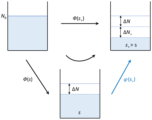
Figure 1In a pool of N0 ice-nucleating particles, ΔN ice crystals form at ice supersaturation s, and ΔN+ additional ice crystals form at a higher value, s+. The resulting ice crystal numbers can be directly predicted from time-independent, cumulative ice-active fractions, ϕ, based on the original INP sample of size N0 (“no budget” approach, black arrows labeled with ϕ). When already activated INPs are removed at s (“budget” approach, curved arrow), ϕ can no longer be used at s+ because of the reduced sample size, (N0−ΔN). This study derives differential ice-active fractions, φ, that can be applied to derive ΔN+ from the smaller sample (blue arrow).
The following issue arises, as illustrated in Fig. 1: after ice has formed on INPs at a given value of s>0, the latter are budgeted (removed) to ensure that the same INPs are no longer available for nucleation. With ΔN newly formed ice crystals, only (N0−ΔN) INPs are available for further nucleation. The number of crystals formed in a succeeding nucleation event at must not be diagnosed from , as the s-cumulative ice-active fraction is based on a sample of N0 particles.
We may estimate the differential AF associated with the step process (Fig. 1). By definition, the number of INPs activating between s and s+ is given by . Therefore, the number of unactivated INPs at s+ is given by the following rate equation:
yielding
The cumulative AF leads to and correspondingly, N0ϕ(s)=ΔN. Therefore, ΔN+ is given by
and the differential AF belonging to the blue arrow in Fig. 1 is expressed solely in terms of the cumulative AF:
In the initial step of ice activation, where s increases from a value ≤0 to s>0 for the first time, Eq. (4) simplifies to φ(s)=ϕ(s), because .
As we show in Sect. 3, using cumulative instead of differential AFs in the “budget” approach shifts the outcome of the competition between homogeneous droplet freezing and heterogeneous ice nucleation on INPs artificially towards the latter. This competition is an important topic in cloud research (Lohmann, 2017; Kärcher, 2017).
We derive differential ice-active fractions (Sect. 3.1) and corresponding particle number budget equations (Sect. 3.2) for phase transitions involving INPs with time-independent nucleation behavior and the ice crystals formed from them. The use of differential spectra derived from immersion freezing experiments is discussed by Vali (2019).
3.1 Differential ice-active fractions
We define a sequence of ice supersaturation values, {sj} (henceforth s-grid), with grid spacings and index , starting at s0=0 with ϕ(s0)=0. To derive differential AFs, it suffices to assume that sj values increase.
We view ϕj≡ϕ(sj) as the statistical outcome of many identically prepared laboratory measurements. While ϕj describes the fraction of INPs that are ice-active within the interval [0,sj], the associated differential AF, φj, shall describe only those INPs that are ice-active within . Therefore, the probability that INPs remain unactivated at sj, (1−ϕj), is given by the product of the probabilities for particles not activating in all intervals Δsℓ prior to sj, (1−φℓ):
φj (j>1) is obtained by recursion (by definition, φ1=ϕ1) from the above equation as follows:
generalizing Eq. (4). Note that differential AFs depend on the type of s-grid. Equation (6) tells us that φj equals the fraction of INPs activated within Δsj in the “no budget” approach, , corrected by a factor accounting for the removal of INPs that are ice-active below sj−1.
Depleting INPs from their reservoir after ice activation as done in cloud models is equivalent to using smaller and smaller samples in laboratory experiments. As a result, the correct AFs to be used in such models, φ, are smaller than ϕ, because the number of unactivated INPs remaining decreases with increasing s. Using ϕ instead increases and biases the number of INP-derived ice crystals. This unphysical effect is to be avoided in models that budget INP and associated ice crystal numbers.
We model cumulative AFs analytically using
with the 50 % activation point, s∗ (), and the slope parameter, δs. Equation (7) allows us to conveniently fit measured cumulative AFs. For instance, Ullrich et al. (2017) provide ϕ for desert dust using an empirical parameterization for the active site density, ns(s,T): . Evaluating this expression at T=220 K and for a surface area, A, of a spherical particle with 1 µm diameter, Eq. (7) provides a reasonable fit with and δs=0.0175 (Appendix A). A more realistic representation of ice activity integrates ϕdust over a surface area distribution of dust particles, which would cause ice to form across a wider range of s values, corresponding to a larger δs value. For illustration, we apply Eq. (7) with and δs=0.05.
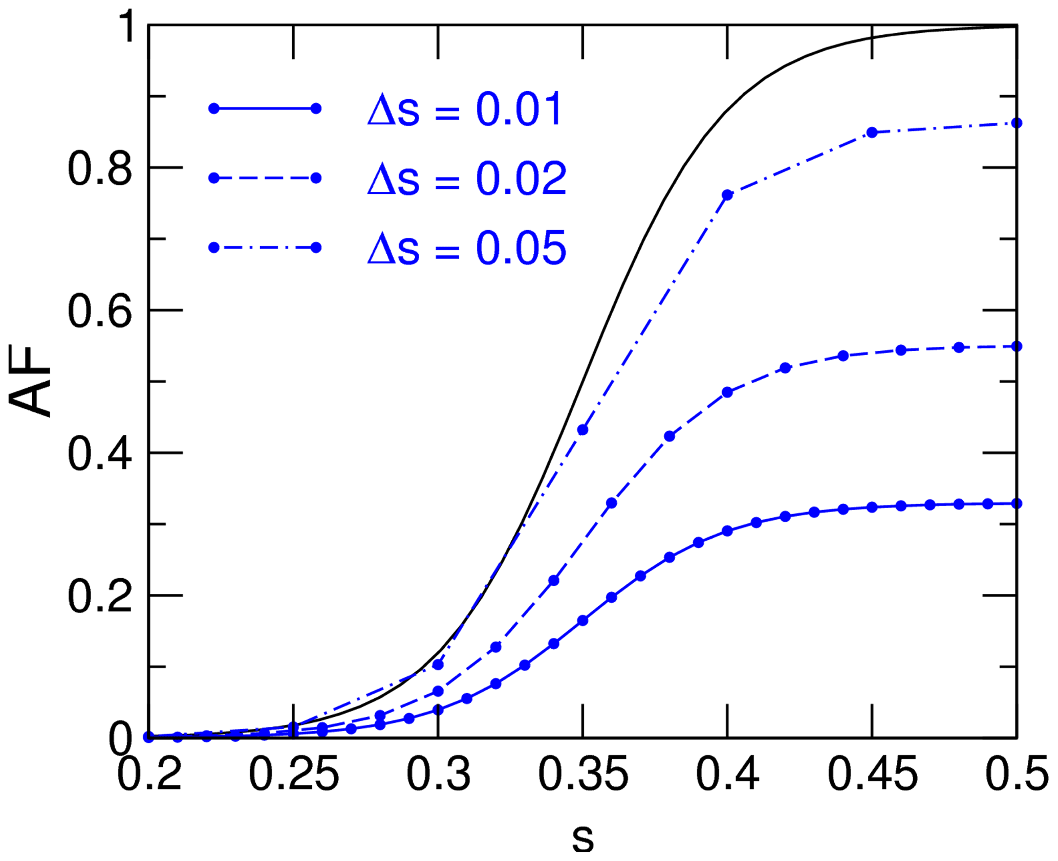
Figure 2The cumulative AF (ϕ, black curve) and associated differential AFs (φ, blue curves) evaluated across three s-grids with constant spacings: Δs=0.01 (solid), Δs=0.02 (dashed), and Δs=0.05 (dot-dashed).
Figure 2 depicts AFs based on Eqs. (6) and (7), evaluated for a linear s-grid with various constant grid spacings, Δs: . Consistent with Eq. (6), φ approaches ϕ for , and φ is significantly lower than ϕ for s≳s∗. As Δs increases and comprises a greater range of s values, differences between cumulative and differential AFs diminish, although at the cost of resolution.
3.2 Particle budgets
In this section, we employ both a linear and sinusoidal s-grid defined by
respectively, where Δs is a constant grid spacing. The linear grid (Eq. 8) describes a monotonically increasing supersaturation history representing a single ice formation event (s increases linearly due to adiabatic cooling for sufficiently small, constant cooling rates). The wavy grid (Eq. 9) illustrates an idealized, non-monotonically rising supersaturation history with rising amplitude envelope (set by Aj), such as encountered during gravity wave activity with alternating cooling and heating cycles (controlled by αj). Both trajectories are shown in Fig. 3a and d.
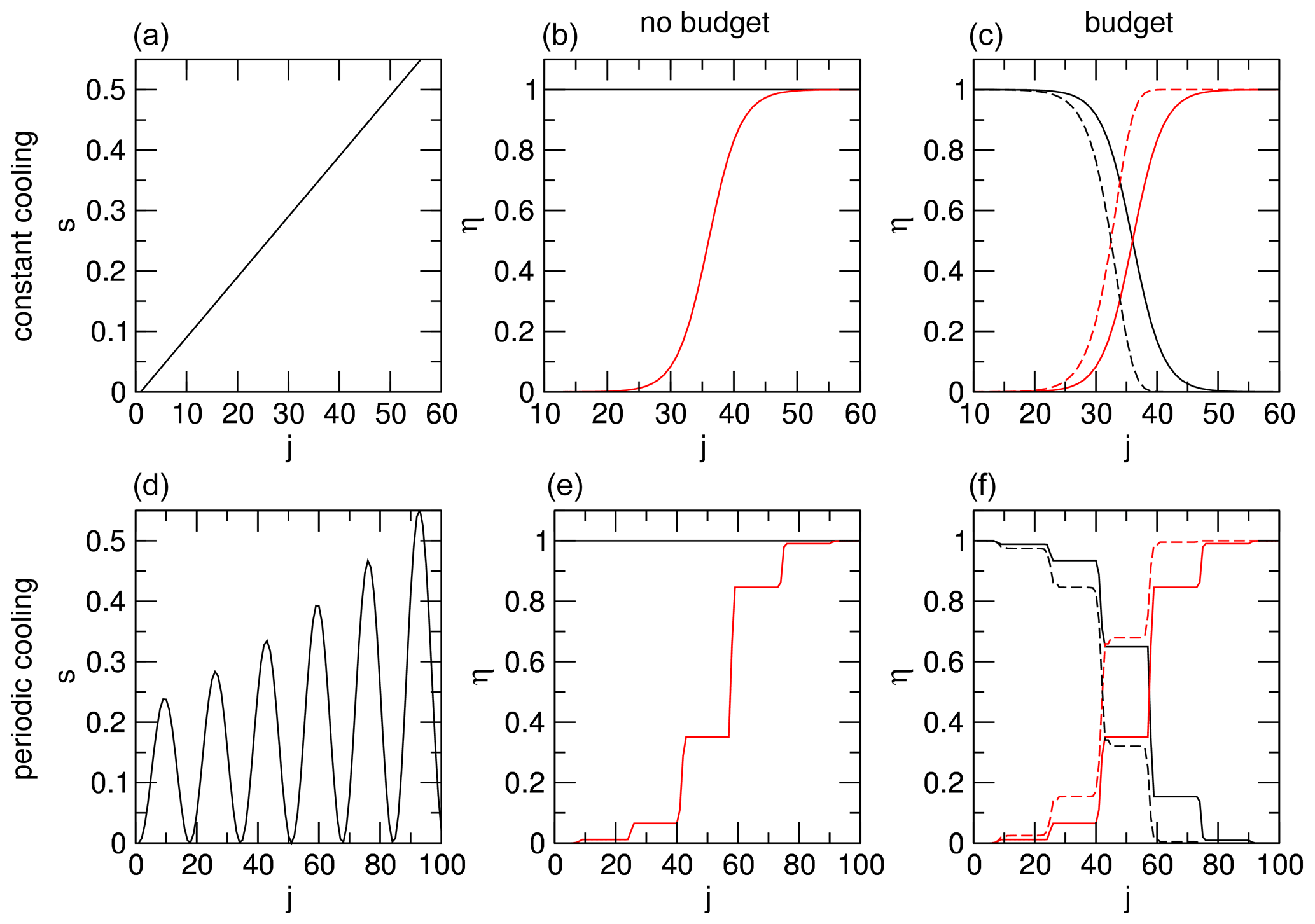
Figure 3Evolution of deterministic ice formation events driven by (a–c) constant cooling and (d–f) periodically oscillating cooling and heating, as indicated by panels (a) and (d), which show ice supersaturation versus dimensionless time. Panels (b), (c), (e), and (f) show the resulting evolution of (black) INP and (red) cumulated ice crystal numbers in a model without and with the budgeting of particle numbers based on the cumulative AF from Eq. (7) with and δs=0.05 and the associated differential AFs, respectively. The dashed curves in the “budget” approach were obtained by wrongly using the cumulative AF so that the difference from the solid curves indicates the error in simulated particle numbers.
To simplify the notation, j shall represent a dimensionless time variable. We note that, in general, each grid representation, {sj}, is subject to its own temporal development. For example, s might additionally be affected by latent heat release or ice crystal growth. In cloud models, where grid spacing and temporal evolution cannot be separated, {sj} is determined by the time steps needed to simulate ice formation. The time steps may vary during the simulation depending on accuracy requirements. The differential AFs from Eq. (6) are then computed based on a variable s-grid.
We denote the number of ice crystals forming from INPs that are ice-active at sj as Ni,j and the corresponding number of remaining (unactivated) INP as Na,j. We normalize both variables by the initial number of INPs (at s=0), N0: , so that they are bounded by zero and one. The equations governing the evolution (j≥1) in the time-independent (deterministic) nucleation framework for both linear and wavy supersaturation histories without budgeting particle numbers are given by
with ϕj taken from Eq. (7) and . By definition, ηi,j values denote cumulative number concentrations. The fact that ηa,j stays constant is consistent with the “no budget” approach. For non-monotonically increasing supersaturation, Δsj take zero or negative values. The function ensures that ice crystal numbers do not decrease when INPs encounter a supersaturation lower than the highest previous value. This reflects the deterministic nature of nucleation on INPs and is in contrast with stochastic homogeneous ice nucleation, where all particles of a given size nucleate ice with the same probability determined by the freezing rate, irrespective of the supersaturation history.
When considering particle number budgets (see Sect. 2), we use differential AFs:
with . The ηa,j values diminish as ice formation progresses while the total particle number, , is conserved (i.e., independent of j). For non-monotonically increasing supersaturation, we modify cumulative AFs by to evaluate φj. This ensures that stays constant, and φj=0 when s values descend from (j−1) to j, as motivated above.
Results for both types of s-grids are presented in Fig. 3, assuming either Δs=0.01 in Eq. (8) or variable grid spacing with jmax=101 in Eq. (9). For constant cooling (Fig. 3a–c), s-cumulative, normalized ice crystal numbers ηi rise continuously and INP numbers ηa stay constant in the “no budget” approach. When ice crystals are budgeted, using the cumulative AF overpredicts ηi, although INPs are removed (ηa decreases). When cooling and heating periods alternate (Fig. 3d–f), ηi again increases at the expense of ηa, but using the cumulative AF together with budgeting ice crystals again leads to an overprediction of ice crystal numbers.
The impact on cloud properties of wrongly using cumulative AFs in specific simulations cannot be judged based on the results shown in Fig. 3 alone. For example, in cirrus simulations, the change in total nucleated ice crystal numbers is likely small in situations with efficient INPs (with large near s∗) and high cooling rates, as most INPs will activate straightaway and the time needed for s to increase above the 50% activation level is short.
A number of models exist to study clouds. Specific cloud processes such as nucleation are simulated in air parcel models on the process level. Cloud-resolving models simulate formation and evolution of clouds with high resolution. Cloud system-resolving models track the life cycles of clouds on regional scales, better accounting for large-scale controls but with poorer resolution and increased need for parameterizations of small-scale processes. Global models with coarse resolution represent much of the atmospheric complexity, but they represent clouds only by way of parameterization. In all types of models, ice-forming aerosol particles and cloud ice crystals may be represented by size-integrated properties, such as total particle number, or contain explicit size information via particle size distributions (PSDs). We compare cumulative and differential AFs with size-resolved or size-integrated INP representation using the example of soot particles as INPs.
Soot particles nucleate ice after processing in mixed-phase clouds and aircraft contrails via PCF (Mahrt et al., 2020). Based on laboratory measurements, soot PCF predicts cumulative AFs of soot aggregates as a function of s and mobility diameter, D (Marcolli et al., 2021). We apply the soot PCF framework to soot particles emitted by aircraft jet engines. We model their PSD, F(D), using a lognormal function (normalized to unity) with an average modal mobility diameter of 32 nm and geometric standard deviation of 1.82, representing average cruise conditions (Zhang et al., 2019). Defining the size distribution of ice-active particles as , size-integrated ice-active fractions (INP spectra, for short) follow from
with ϕ(s,D) taken from Marcolli et al. (2021).
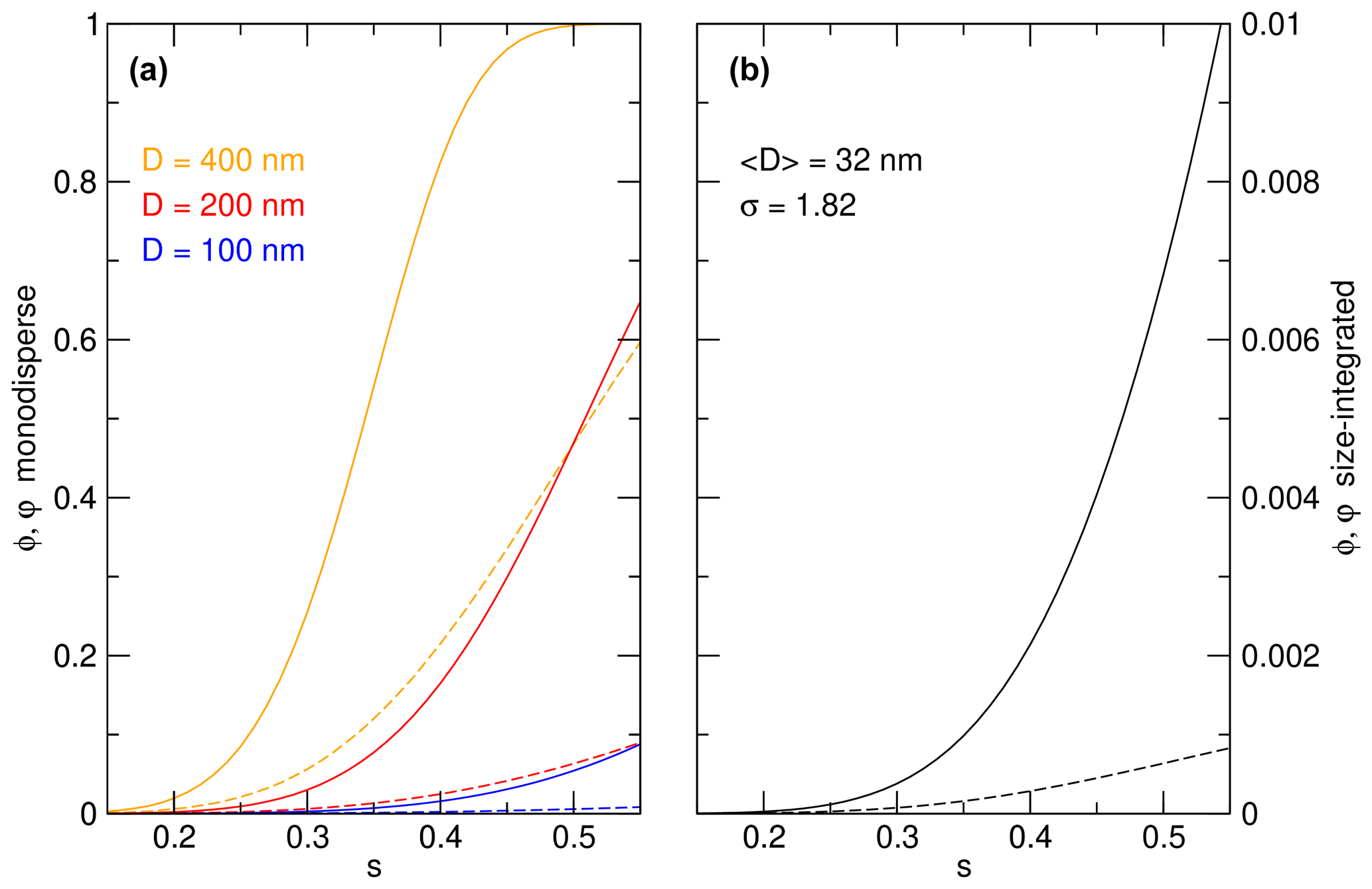
Figure 4(a) The cumulative (solid curves) and differential AFs (dashed curves) for contrail-processed aircraft soot particles with mobility diameters of (orange) 400, (red) 200, and (blue) 100 nm. (b) The cumulative (solid) and differential (dashed) AFs integrated over a population of contrail-processed aircraft soot particles with lognormal number size distribution parameters indicated in the legend. Differential AFs are computed based on an s-grid with constant spacing Δs=0.01.
Figure 4 shows size-resolved and size-integrated cumulative and differential AFs of aircraft soot particles processed in contrails (Kärcher et al., 2021). Size-resolved cumulative AFs decrease strongly with mobility diameter from 400 to 100 nm and reduce to zero for D<40 nm (not shown). As the soot PSD peaks in the Aitken size range, size-integrated ice activity is low (<0.01) even at high ice supersaturation (s=0.5).
A general recommendation on how to include differential AFs in models cannot be given, as this depends on details of the numerical implementation of aerosol–cloud interactions, especially in global models with long time steps where INP budgets are affected by both microphysics and transport. However, differential AFs are straightforward to implement in cloud models when making use of the budget Eqs. (12) and (13) in combination with Eq. (6). Cumulative AFs may be used only in studies of single ice formation events, which do not require the removal of INPs after nucleation, e.g., in parameterizations and underlying parcel simulations.
Water phase transitions in clouds induced by INPs with deterministic ice nucleation behavior are described by time-independent AFs that are cumulative in ice supersaturation. In prognostic cloud models, care must be taken to avoid the simulation of multiple ice formation events from the same particles. This is accomplished by the introduction of budget equations for INPs and the ice crystals deriving from them. While straightforward in the case of time-dependent budget equations (suitable for stochastic freezing) containing source and sink terms for the number of aerosol particles (or cloud droplets) and ice crystals, a similar approach is not feasible in the case of INPs with singular ice nucleation behavior. We formulated differential AFs consistent with the removal of such INPs after activation and introduced modifications that are necessary when ice supersaturation evolves non-monotonically over time. We discussed the representation of ice activation in cloud models and showed that using differential AFs prevents the overestimation of INP effects. Finally, we demonstrated the importance of including INP size information in estimations of AFs.
Our insights help improve cloud simulations and better understand the relative roles of natural and anthropogenic INPs in determining coverage, lifetime, and radiative response of mid- and high-level clouds.
The hyperbolic tangent chosen to represent ϕ allows one to easily compare measured and parameterized s-cumulative ice-active fractions and perform sensitivity studies. It is based on only two parameters, s∗ and δs, with clear physical significance (Sect. 3.1). Here, we apply this function to fit the activation curve from Ullrich et al. (2017) for monodisperse (1 µm) spherical dust particles using and δs=0.0175.
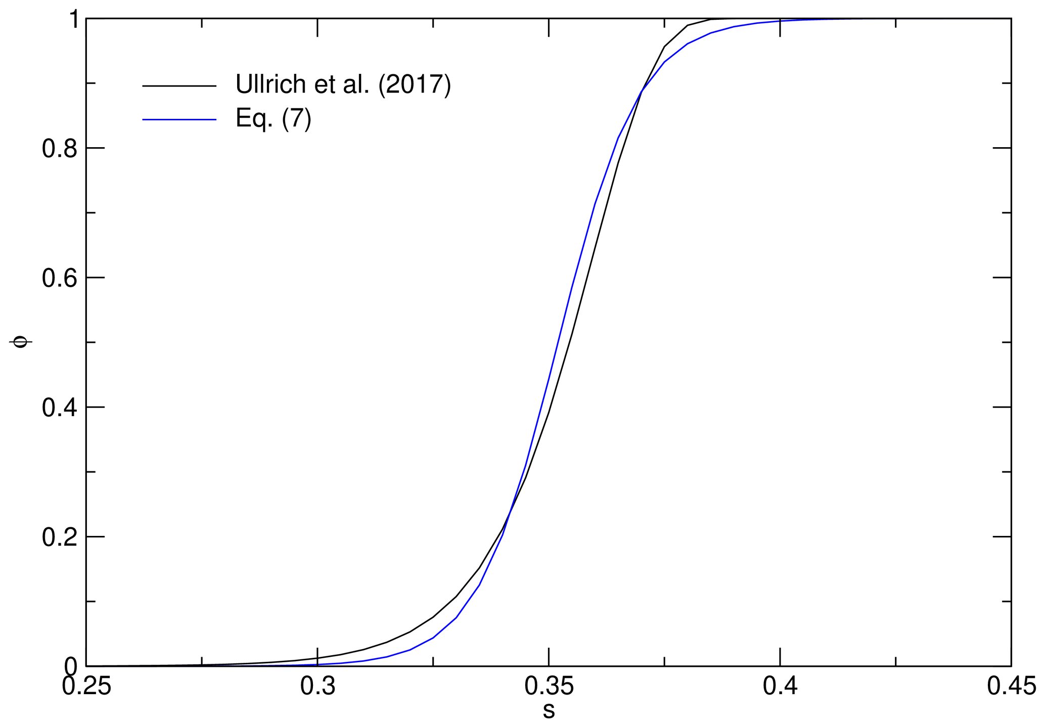
Figure A1Comparison of an ice activation parameterization for 1 µm dust particles (black curve) with an analytical approximation (blue).
Figure A1 shows that Eq. (7) approximates the parameterization very well, especially in the crucial part around s∗, where ϕ rises steeply from low to significant values. We presume that the hyperbolic tangent provides reasonable fits to activation curves of other INP types as well, which show a similar s dependence. We note that the parameter values suitable for monodisperse particles change when size-dependent cumulative ice-active fractions are integrated over a particle size distribution.
In discussing deterministic ice formation (Sect. 3), we have chosen a larger slope parameter, δs=0.05. This spreads ice activation over a larger range of s values (compare the black curve from Fig. 2 with the blue curve from Fig. A1) and helps illustrate the ice activation events shown in Fig. 3 more clearly.
The data that support the findings of this study are available on Zenodo: https://doi.org/10.5281/zenodo.5560883 (Kärcher and Marcolli, 2021).
BK conceived of the study, performed the calculations, and drafted the manuscript. CM developed the concept of differential ice-active fractions, discussed ice nucleation measurements, and contributed to writing the final paper.
The contact author has declared that neither they nor their co-author has any competing interests.
Publisher's note: Copernicus Publications remains neutral with regard to jurisdictional claims in published maps and institutional affiliations.
The article processing charges for this open-access publication were covered by the German Aerospace Center (DLR).
This paper was edited by Susannah Burrows and reviewed by two anonymous referees.
Cziczo, D. J., Ladino, L., Boose, Y., Kanji, Z. A., Kupiszweski, P., Lance, S., Mertes, S., and Wex, H.: Measurements of ice nucleating particles and ice residuals, Meteor. Mon., 58, 8.1–8.13, https://doi.org/10.1175/AMSMONOGRAPHS-D-16-0008.1, 2017. a
David, R. O., Marcolli, C., Fahrni, J., Qiu, Y., Sirkin, Y. A. P., Molinero, V., Mahrt, F., Brühwiler, D., Lohmann, U., and Kanji, Z. A.: Pore condensation and freezing is responsible for ice formation below water saturation for porous particles, P. Natl. Acad. Sci. USA, 116, 8184–8189, https://doi.org/10.1073/pnas.1813647116, 2019. a
Holden, M. A., Whale, T. F., Tarn, M. D., O'Sullivan, D., Walshaw, R. D., Murray, B. J., Meldrum, F. C., and Christenson, H. K.: High-speed imaging of ice nucleation in water proves the existence of active sites, Sci. Adv., 5, 2, https://doi.org/10.1126/sciadv.aav4316, 2019. a
Kanji, Z. A., Ladino, L. A., Wex, H., Boose, Y., Burkert-Kohn, M., Cziczo, D. J., and Krämer, M.: Overview of ice nucleating particles, Meteor. Mon., 58, 1.1–1.33, https://doi.org/10.1175/AMSMONOGRAPHS-D-16-0006.1, 2017. a
Kärcher, B.: Cirrus clouds and their response to anthropogenic activities, Current Climate Change Reports, 3, 45–57, https://doi.org/10.1007/s40641-017-0060-3, 2017. a
Kärcher, B. and Marcolli, C.: Aerosol–cloud interactions: the representation of heterogeneous ice activation in cloud models, Zenodo [data set], https://doi.org/10.5281/zenodo.5560883, 2021. a
Kärcher, B., Mahrt, F., and Marcolli, C.: Process-oriented analysis of aircraft soot-cirrus interactions constrains the climate impact of aviation, Communications Earth & Environment, 2, 113, https://doi.org/10.1038/s43247-021-00175-x, 2021. a
Kaufmann, L., Marcolli, C., Luo, B., and Peter, T.: Refreeze experiments with water droplets containing different types of ice nuclei interpreted by classical nucleation theory, Atmos. Chem. Phys., 17, 3525–3552, https://doi.org/10.5194/acp-17-3525-2017, 2017. a
Kiselev, A., Bachmann, F., Pedevilla, P., Cox, S. J., Michaelides, A., Gerthsen, D., and Leisner, T.: Active sites in heterogeneous ice nucleation – the example of K-rich feldspars, Science, 355, 367–371, https://doi.org/10.1126/science.aai8034, 2017. a
Lohmann, U.: Anthropogenic aerosol influences on mixed-phase clouds, Current Climate Change Reports, 3, 32–44, https://doi.org/10.1007/s40641-017-0059-9, 2017. a
Mahrt, F., Kilchhofer, K., Marcolli, C., Grönquist, P., David, R. O., Rösch, M., Lohmann, U., and Kanji, Z. A.: The impact of cloud processing on the ice nucleation abilities of soot particles at cirrus temperatures, J. Geophys. Res., 125, e2019JD030922, https://doi.org/10.1029/2019JD030922, 2020. a
Marcolli, C.: Deposition nucleation viewed as homogeneous or immersion freezing in pores and cavities, Atmos. Chem. Phys., 14, 2071–2104, https://doi.org/10.5194/acp-14-2071-2014, 2014. a
Marcolli, C.: Technical note: Fundamental aspects of ice nucleation via pore condensation and freezing including Laplace pressure and growth into macroscopic ice, Atmos. Chem. Phys., 20, 3209–3230, https://doi.org/10.5194/acp-20-3209-2020, 2020. a, b
Marcolli, C., Mahrt, F., and Kärcher, B.: Soot PCF: pore condensation and freezing framework for soot aggregates, Atmos. Chem. Phys., 21, 7791–7843, https://doi.org/10.5194/acp-21-7791-2021, 2021. a, b, c
Peckhaus, A., Kiselev, A., Hiron, T., Ebert, M., and Leisner, T.: A comparative study of K-rich and Na/Ca-rich feldspar ice-nucleating particles in a nanoliter droplet freezing assay, Atmos. Chem. Phys., 16, 11477–11496, https://doi.org/10.5194/acp-16-11477-2016, 2016. a
Tarn, M. D., Sikora, S. N. F., Porter, G. C. E., O'Sullivan, D., Adams, M., Whale, T. F., Harrison, A. D., Temprado, J. V., Wilson, T. W., Shim, J., and Murray, B. J.: The study of atmospheric ice-nucleating particles via microfluidically generated droplets, Microfluid. Nanofluid., 22, 52, https://doi.org/10.1007/s10404-018-2069-x, 2018. a
Ullrich, R., Hoose, C., Möhler, O., Niemand, M., Wagner, R., Höhler, K., Hiranuma, N., Saathoff, H., and Leisner, T.: A new ice nucleation active site parameterization for desert dust and soot, J. Atmos. Sci., 74, 699–717, https://doi.org/10.1175/JAS-D-16-0074.1, 2017. a, b
Vali, G.: Revisiting the differential freezing nucleus spectra derived from drop-freezing experiments: methods of calculation, applications, and confidence limits, Atmos. Meas. Tech., 12, 1219–1231, https://doi.org/10.5194/amt-12-1219-2019, 2019. a, b
Vali, G., DeMott, P. J., Möhler, O., and Whale, T. F.: Technical Note: A proposal for ice nucleation terminology, Atmos. Chem. Phys., 15, 10263–10270, https://doi.org/10.5194/acp-15-10263-2015, 2015. a, b
Zhang, X., Chen, X., and Wang, J.: A number-based inventory of size-resolved black carbon particle emissions by global civil aviation, Nat. Commun., 10, 534, https://doi.org/10.1038/s41467-019-08491-9, 2019. a
- Abstract
- Introduction
- Stating the issue
- Solving the issue
- Applying ice-active fractions in models across scales
- Concluding remark
- Appendix A: Analytical representation of ice-active fractions
- Data availability
- Author contributions
- Competing interests
- Disclaimer
- Financial support
- Review statement
- References