Mass and density of individual frozen hydrometeors

A new precipitation sensor, the Differential Emissivity Imaging Disdrometer (DEID), is used to provide the first continuous measurements of the mass, diameter, and density of individual hydrometeors. The DEID consists of an infrared camera pointed at a heated aluminum plate. It exploits the contrasting thermal emissivity of water and metal to determine individual particle mass by assuming that energy is conserved during the transfer of heat from the plate to the particle during evaporation. Particle density is determined from a combination of particle mass and morphology. A Multi-Angle Snowflake Camera (MASC) was deployed alongside the DEID to provide refined imagery of particle size and shape. Broad consistency is found between derived mass–diameter and density–diameter relationships and those obtained in prior studies. However, DEID measurements show a generally weaker dependence with size for hydrometeor density and a stronger dependence for aggregate snowflake mass.

1 Introduction

Predictions of precipitation amount, location, and duration have been shown to be especially sensitive to parameterized expressions for how fast a hydrometeor falls (Rutledge and Hobbs, 1984; Reisner et al., 1998; Hong et al., 2004; Fovell and Su, 2007; Lin et al., 2010; Liu et al., 2011; Iguchi et al., 2012; Thériault et al., 2012), affecting forecasts of hurricane trajectories (Fovell and Su, 2007) and storm lifetimes (Garvert et al., 2005; Colle et al., 2005; Milbrandt et al., 2010). From the perspective of fluid dynamics, fall speed can be related to the mass and density of precipitation particles (Böhm, 1989). Observationally, one of the most frequently cited datasets that lies at the heart of current bulk microphysical parameterizations (e.g. Reisner et al., 1998; Hong et al., 2004; Tao et al., 2003) comprises just 376 snowflakes captured and photographed in the Cascade mountain range. Individual hydrometeors were melted on a sheet of plastic film, from which relationships were obtained between hydrometeor mass, fall speed, and diameter as a function of particle habit and, in the case of graupel, density (Locatelli and Hobbs, 1974). Despite its limited scope, later numerical studies (Böhm, 1989; Khvorostyanov and Curry, 2002; Heymsfield and Westbrook, 2010; Kubicek and Wang, 2012) and ground-based disdrometer measurements (Kruger and Krajewski, 2002; Barthazy et al., 2004; Yuter et al., 2006; Newman et al., 2009) have lent general support to this reference dataset, although concerns remain about geographic and temporal specificity, measurement limitations (Yuter et al., 2006; Battaglia et al., 2010), and the ability to quantify the extent of riming (Barthazy and Schefold, 2006; Brandes et al., 2008).

Particle density measurements have proven more difficult to ascertain as they require, in addition to mass, an estimate of particle volume. This may be reasonably obtained for quasi-spherical particles such as lump graupel (Locatelli and Hobbs, 1974), but the task is considerably more challenging when snow particles are formed from ice crystal aggregation. A possible approach is to infer density from fallen snow using column measurements (Conger and McClung, 2009), capacitance probes (Dent et al., 1998), or a combination of a camera for snow depth and an electric scale for snow mass (Muramoto et al., 1995). Muramoto et al. (1995) and Brandes et al. (2007) measured the bulk mass of snowflakes using a weighing gauge, from which the bulk volume was determined with 2D camera imagery of individual snowflakes. Tiira et al. (2016) determined a volume flux weighted snow density for a population of snowflakes using particle size distribution, fall speed, and a weighing gauge to estimate the mass, as well as 2D camera imagery to determine effective diameter and volume. However, snow undergoes compaction and melting on the ground; thus, the relationship to individual particle density in the air is approximate (Brun et al., 1992). To obtain individual snowflake particle density, Magono and Nakamura (1965) collected individual wet and dry snowflakes on a piece of dyed filter paper, from which the outline of the flake was manually measured. Individual volume was inferred from the major and minor axes of the outline of snow and the mass from the outline of the melted snowflake. Holroyd (1971) also made measurements of the major and minor axes of powder snow and dendrites from (Magono and Nakamura, 1965). A limitation of these datasets is that they were necessarily small given the manual nature of the effort.

Here, we present continuous measurements of individual masses of frozen hydrometeors using a new instrument, the Differential Emissivity Imaging Disdrometer (DEID). DEID data (Rees et al., 2021) are combined with photographic imagery obtained using a Multi-Angle Snowflake Camera (MASC) (Garrett et al., 2012) to obtain estimates of particle density.

2 Methods

All measurements described in this study were acquired at a meteorological measurement tower placed at the mouth of Red Butte Canyon (40.76857, −111.82614) in Salt Lake City, Utah, at 1547 m elevation in January and February 2020. More details about the site and measurement campaign are provided by Singh et al. (2021).

2.1 Particle mass from thermal imaging

The Differential Emissivity Imaging Disdrometer (DEID) (Singh et al., 2021) consists of a thermal camera operating at a frequency between 2 and 12 Hz pointed at an aluminum plate placed atop a hotplate maintained at a self-sustained temperature of 85 ^∘C. The camera distinguishes hydrometeors as they melt and evaporate as white regions on a black background (Fig. 1) due to the contrasting infrared emissivities of water (ϵ≈0.96) and aluminum (ϵ≈0.03). A small strip of polyimide tape (ϵ≈0.95) is applied to the aluminum plate to provide a reference temperature, as well as a pixel-to-length dimension conversion based on the tape's known width. The effective collection area of the DEID was A ≈ 7 cm × 5 cm, and the per pixel resolution of imaged particles p was 190 µm. Processing of the thermal camera imagery yields the hydrometeor area on the plate, the temperature difference between the water and the plate, and the evaporation time.

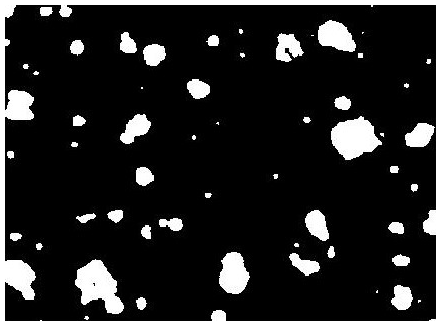
Figure 1 Thermal camera imagery from the DEID, showing regions of high-emissivity water (white) on a low-emissivity aluminum plate (black).

Individual particle mass is determined using the DEID by employing the assumption that the heat gained by a hydrometeor is equivalent to the heat lost by the plate during the process of melting and evaporation. The heat balance equation is

$$\begin{array}{}\text{(1)}& c_p\mathrm{\Delta }T\int \mathrm{d}M+L_{\mathrm{eqv}}\int \mathrm{d}M=\underset{\mathrm{0}}{\overset{t}{\int }}{\displaystyle \frac{K}{H}}A\left(t\right)(T_{\mathrm{p}}-T_{\mathrm{w}}(t\left)\right)\mathrm{d}t,\end{array}$$

where c_p is the specific heat capacity of water at constant pressure, ΔT is the difference in temperature between 0 and time (t), M is the mass of the hydrometeor, and L_eqv is the equivalent latent heat required for the conversion of the hydrometeor to gas. For liquid precipitation, L_eqv=L_v, where L_v is the latent heat of vaporization of water. For solid precipitation, $L_{\mathrm{eqv}}=L_{\mathrm{v}}+L_{\mathrm{f}}$, where L_f is the latent heat fusion for water. K is the thermal conductivity of the aluminum plate, H is the plate thickness, A(t) is the cross-sectional area of the water droplet at time t, T_p is the temperature of the hotplate, and T_w(t) is the temperature of the water at time t. Taking

$$\int \mathrm{d}M=K_{\mathrm{d}}\underset{\mathrm{0}}{\overset{t}{\int }}A\left(t\right)(T_{\mathrm{p}}-T_{\mathrm{w}}(t\left)\right)\mathrm{d}t,$$

a single calibrated constant K_d for the plate was determined experimentally by applying known masses of water from a micropipette to the plate (see Appendix A for the derivation of K_d). The heat balance equation was found in a laboratory setting to be highly insensitive to ambient winds, temperature, and humidity (Singh et al., 2021).

The temperature difference between the plate and water on the plate ($\mathrm{\Delta }T=T_{\mathrm{p}}-T_{\mathrm{w}}\left(t\right)$) can be determined using the mean pixel intensity of the particle in the thermal camera imagery (see Appendix B). The mass calculation then simplifies to

$$\begin{array}{}\text{(2)}& M=K_d\mathrm{\Delta }T\int A\left(t\right)\mathrm{d}t.\end{array}$$

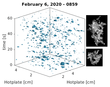
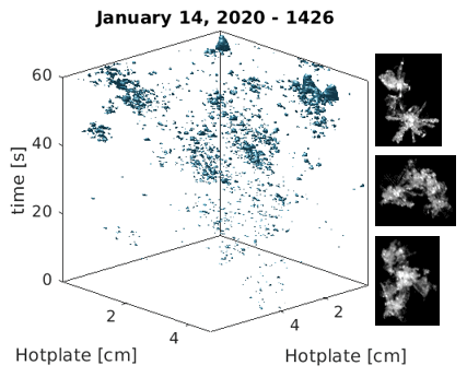
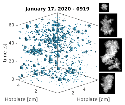
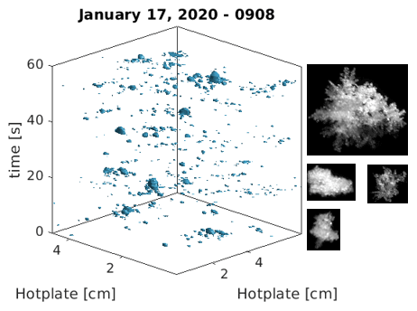
Three-dimensional regions integrated over particle area and evaporation time were constructed for each particle during the melting process defined by $V_t=\int A\left(t\right)\mathrm{d}t$ so that from Eq. (2), M=K_dV_tΔT. An example of a 1 min time interval with 3D volumetric regions representing each individual particle is shown in Fig. 2 for graupel. Additional 3D representations for other snowflake types are shown in Appendix B.

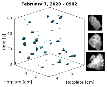
Figure 2 Evaporation volumetric profiles on the DEID plate in a space of imaged area and time $V_t=\int A\left(t\right)\mathrm{d}t$ for graupel.

2.2 Hydrometeor photography

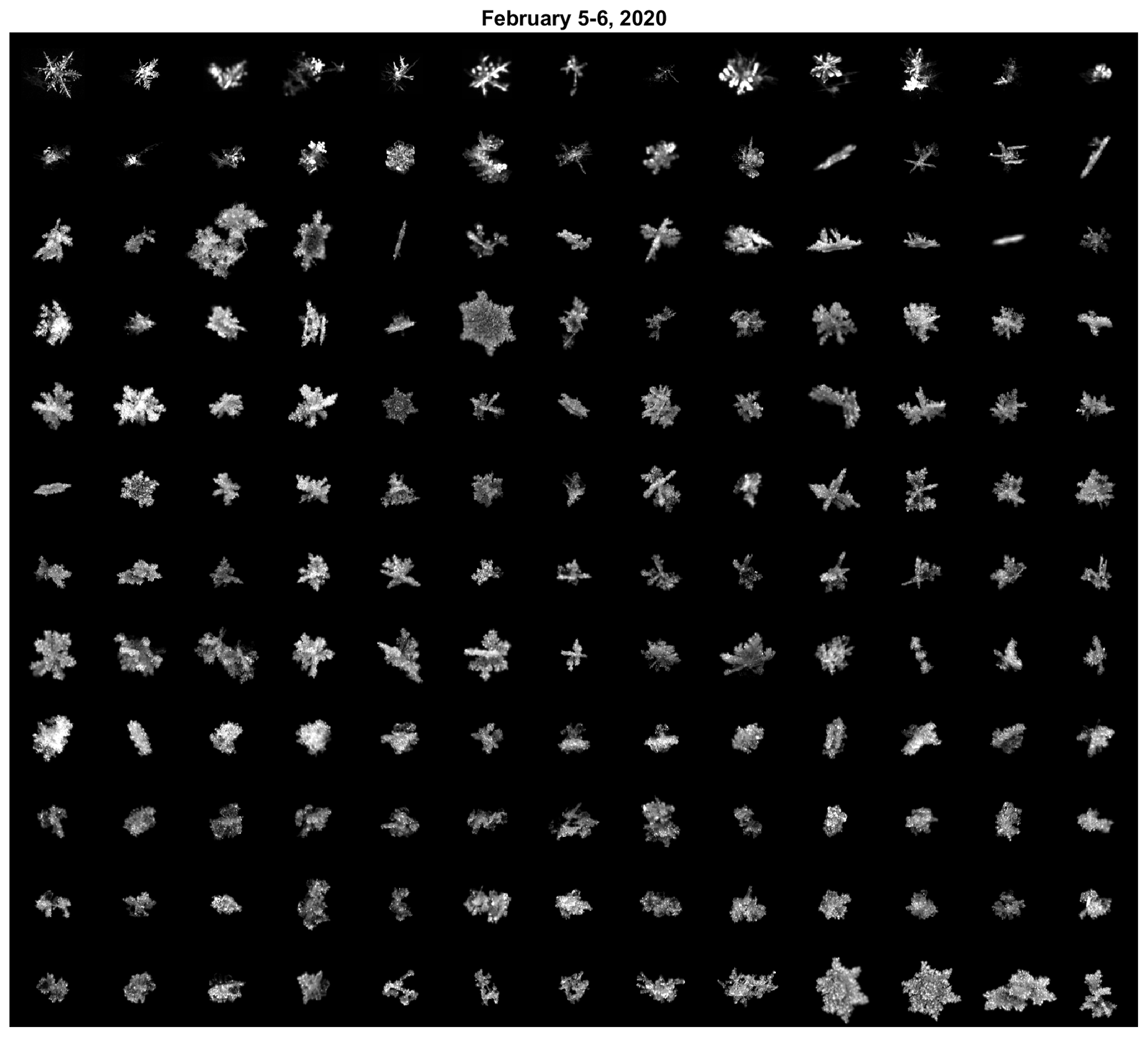
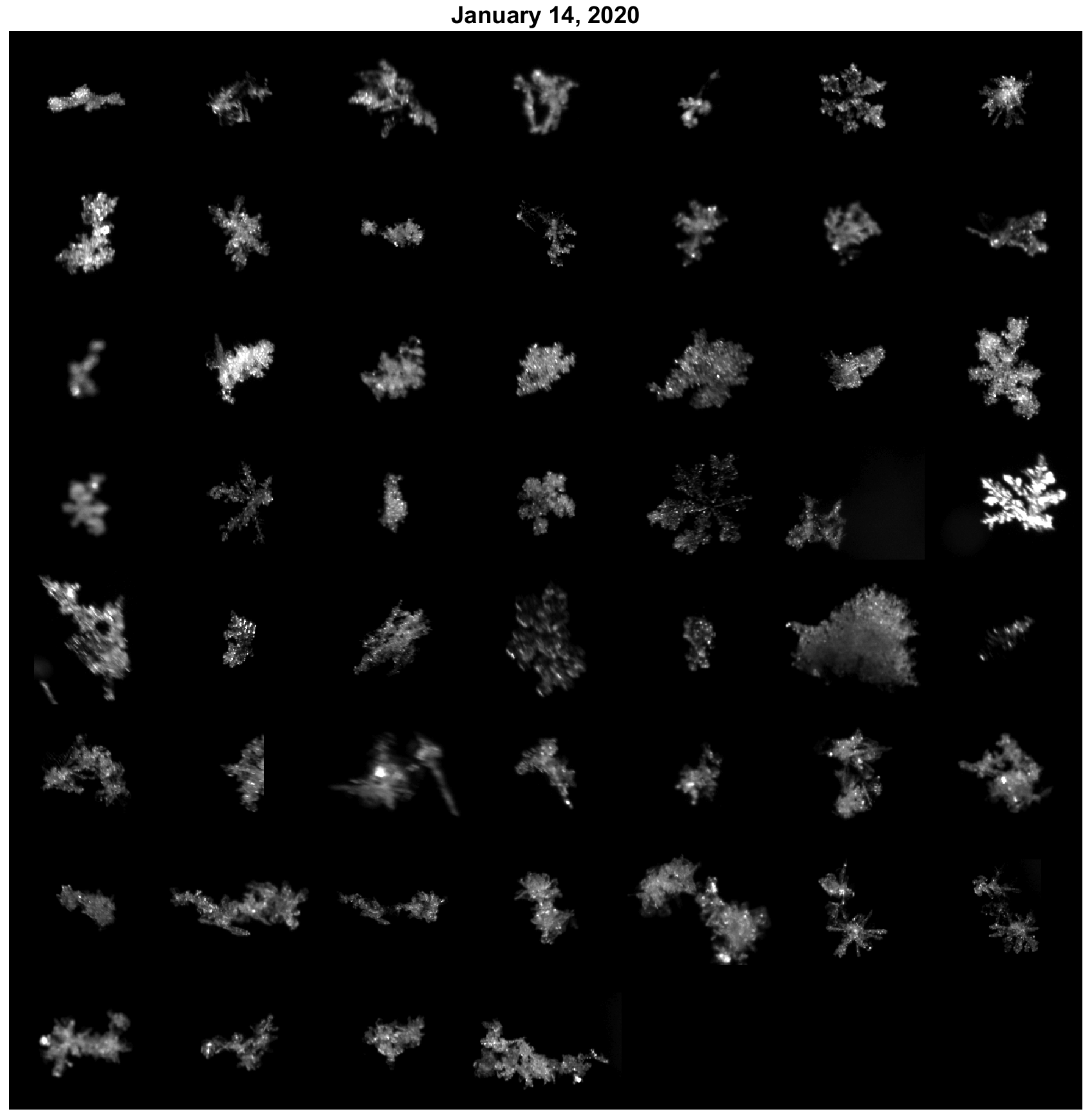
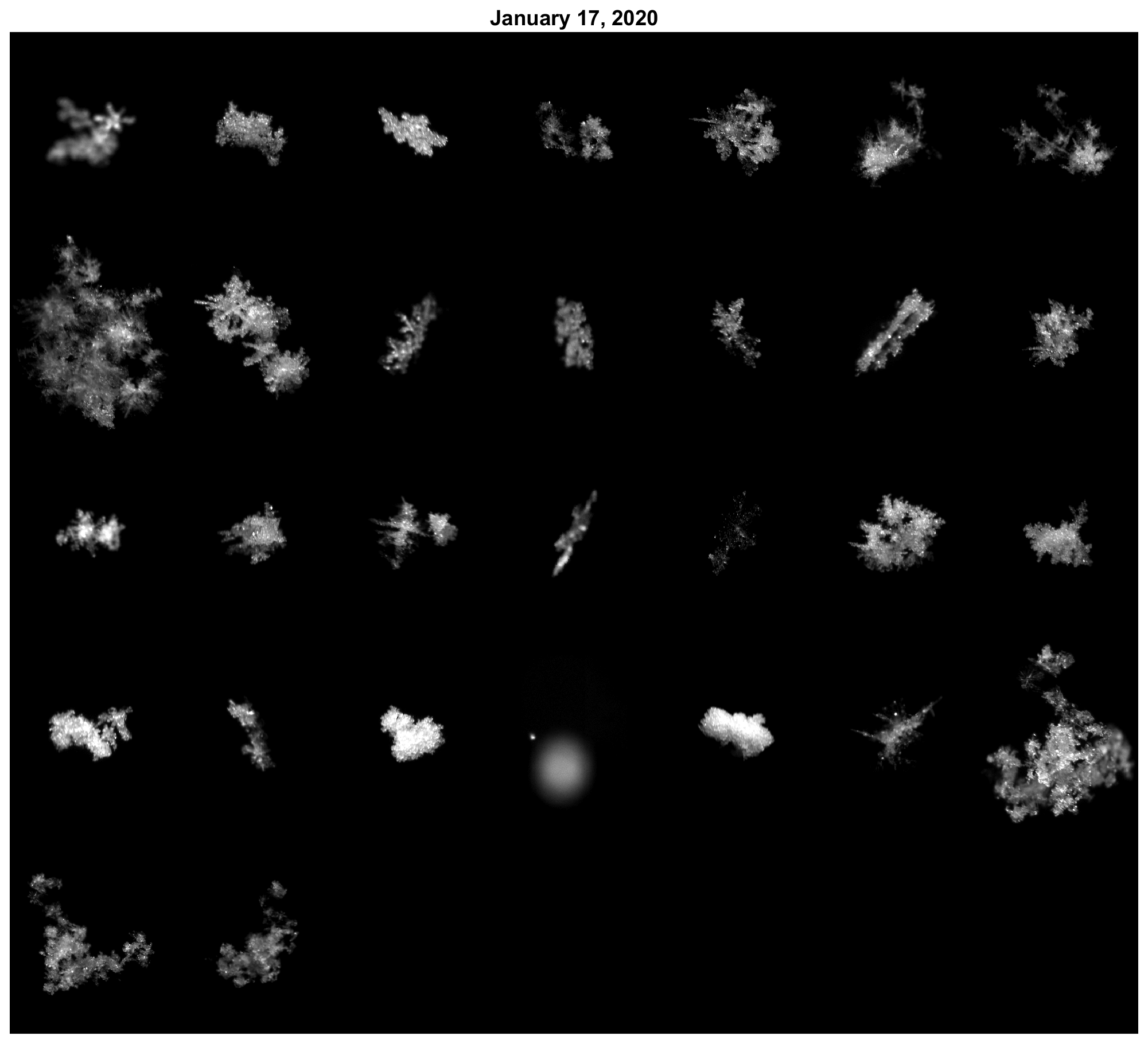
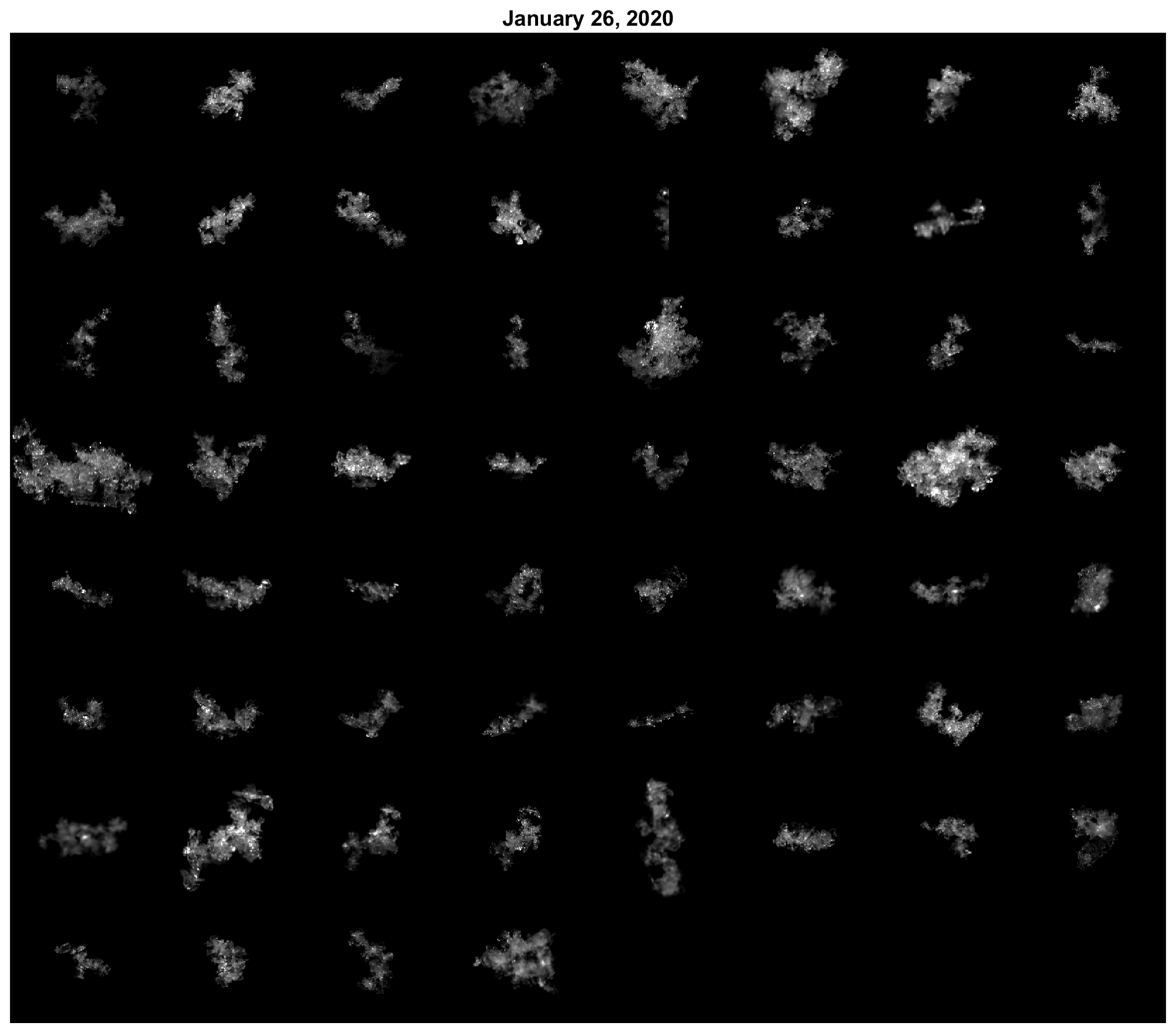
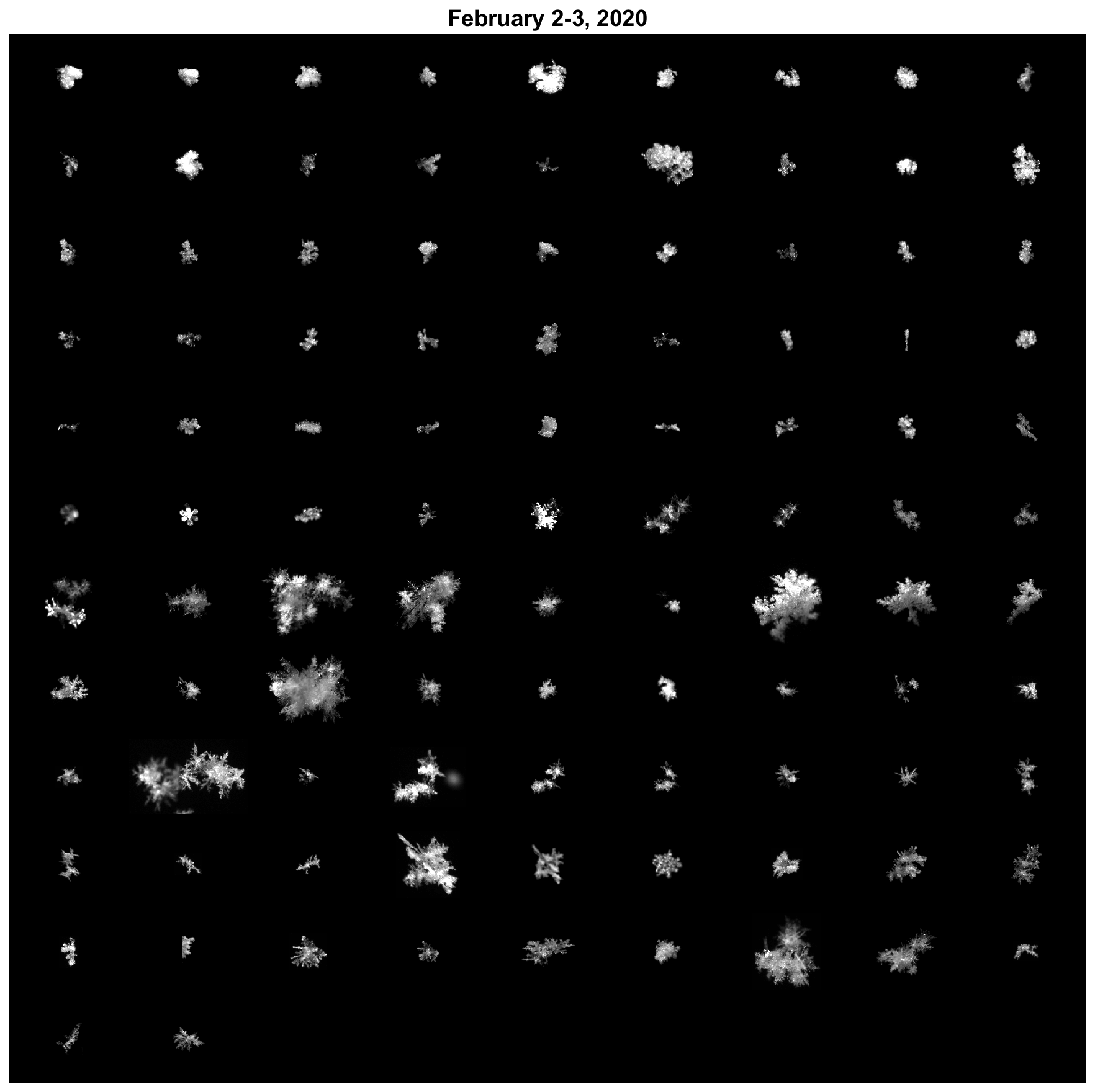
The Multi-Angle Snowflake Camera (MASC) (Garrett et al., 2012) houses three high-speed visible-spectrum cameras arranged concentrically with a separation angle of 36^∘. As a particle falls through the instrument collection aperture, two vertically spaced infrared detectors simultaneously trigger the cameras to take three simultaneous photographs of the particle from the side and to measure the fall speed between the two detectors. The MASC software processes the imagery to calculate the surface area, geometric cross section, perimeter, orientation, aspect ratio, complexity, flatness, and whether the particle is a raindrop (Shkurko et al., 2016). Images taken by the Multi-Angle Snowflake Camera (MASC) are used in conjunction with the DEID to confirm precipitation type and refine density measurements. A mosaic of MASC images from 5 and 6 February 2020 is shown in Fig. 3. Additional snowflake imagery catalogued from each storm is shown in Appendix C.

Figure 3 A selection of MASC snowflake images obtained between 5 and 6 February 2020.

2.3 Particle volume and density

Immediately following the arrival of a hydrometeor on the plate, the particle cross-sectional area increases rapidly as the hydrometeor adjusts from the ambient air temperature to the temperature of the plate, melting in the process. It reaches a maximum cross-sectional area A_max before shrinking during evaporation. A particle may be melted at the moment that it reaches A_max. Nonetheless, due to surface tension, particles that are initially frozen tend to maintain their shape following melting so that A_max is approximately representative of the frozen cross-sectional area in air. In calibration, Singh et al. (2021) found that snowflakes undergo only a 5 % change in D_eff during the melting process.

To obtain an estimate of particle density from particle mass, a spherical volume V_S for each hydrometeor can be estimated from an effective diameter D_eff derived from the A_max. $V_{\mathrm{S}}=\frac{\mathit{\pi }}{\mathrm{6}}{D}_{\mathrm{eff}}^{\mathrm{3}}$, where $D_{\mathrm{eff}}=\sqrt{\frac{\mathrm{4}}{\mathit{\pi }}{A}_{\max }}$ (Fig. 4, left). This geometric definition is consistent with that taken by Locatelli and Hobbs (1974), who prescribed D_eff as “the diameter of the smallest circle into which the aggregate as photographed will fit without changing its density”. Unless otherwise specified, all instances of “diameter” in the text refer to D_eff. An alternative diameter metric is D_max as defined by the circumscribed diameter from the maximum horizontal dimension of the hydrometeor as it lies on the hotplate. The measured relationship between these two metrics is described in Sect. 3.2.

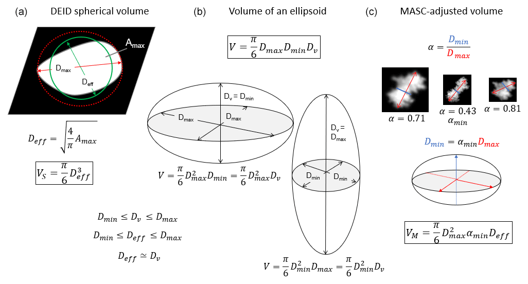
Figure 4 Illustration of the diameter and volume calculations by the DEID (a), maximum and minimum theoretical bounds of volume calculations of spheroids (b), and the corresponding volume adjustment using MASC-derived aspect ratio measurements (c).

For a more precise estimate of particle volume, side-viewing MASC imagery of hydrometeors can be used to determine the average aspect ratios of hydrometeors measured over a 1 min time interval. In general, by approximating hydrometeors as an ellipsoid, the volume of a snowflake is $V_M=\frac{\mathit{\pi }}{\mathrm{6}}{D}_{\max }{D}_{\min }{D}_{\mathrm{v}}$, where D_max is the longest dimension as seen by the DEID, D_min is the shortest, and D_v is bounded by the two. For example, if the hydrometeor shape is an oblate spheroid, then D_v = D_max, and if it is a prolate spheroid, then D_v = D_min (Fig. 4, middle). As a snowflake falls onto the plate, the maximum dimension is expected to lie flat with respect to the plate. D_eff is expected to lie between the maximum and minimum dimensions of the snowflake; thus, for the more general case of an ellipsoid, a reasonable assumption is that D_v≃D_eff.

The issue here is that the DEID is unlikely to provide a measure of the minimum dimension. However, it can be reasonably inferred from side views of hydrometeors provided by the multiple concentric images captured by the MASC. For a given snowflake, the minimum of the aspect ratios for each hydrometeor seen by the multiple MASC cameras as captured within a 1 min interval and subsequently averaged α_min can reveal a characteristic minimum dimension in the vertical direction for the time period that is otherwise invisible to the DEID (Fig. 4, right). Taking D_min=α_minD_max, the MASC-adjusted volume is then

$$\begin{array}{}\text{(3)}& V_M={\displaystyle \frac{\mathit{\pi }}{\mathrm{6}}}{D}_{\max }^{\mathrm{2}}{D}_{\mathrm{eff}}{\mathit{\alpha }}_{\min }.\end{array}$$

The spherical and mass-adjusted density of individual hydrometeors can then be calculated from the mass M and volume as ${\mathit{\rho }}_{\mathrm{S}}=M/V_S$ and ${\mathit{\rho }}_M=M/V_M$ respectively.

3 Results

Over the course of five storms that took place in Salt Lake City, Utah, on 14, 17, and 26 January as well as 2–3 and 5–6 February 2020, the DEID detected 132 459 individual hydrometeors. Of those hydrometeors, 104 812 were snowflakes, and the remainder were either rain or a rain–snow mix. A filtering algorithm rejected small hydrometeors with fewer than three contiguous pixels of data in all three dimensions (see Appendix B), leaving a total dataset (Rees et al., 2021) of 109 316 hydrometeors, of which 86 285 were snowflakes and the remainder rain. Of those snowflakes, density estimates for 43 649 were obtained using corresponding MASC imagery. The density of rain of course is known to be 1000 kg m⁻³ and would provide a valuable reference point for this study. Unfortunately, its measurements cannot be addressed using the techniques described here as raindrops do not preserve their area after impaction on the plate.

3.1 Time series

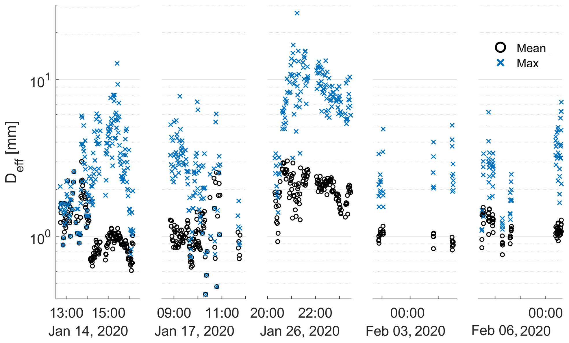
Figure 5 shows the mean and the maximum effective diameters of the hydrometeors considered for each 1 min sampling interval. The largest observed maximum diameters occurred during 14 and 26 January, when large aggregates were the primary snow type (see Appendix C for corresponding snowflake imagery). During such periods characterized primarily by aggregate snowflakes, a larger difference was observed between the mean and maximum diameter observed. Periods characterized primarily by graupel, including early 14 and late 17 January, exhibited smaller differences.

Figure 5 One-minute averaged maximum and mean effective diameters of measured hydrometeors.

Adopting either the spherical volume or the MASC-adjusted volume, the probability density functions for ρ_S and ρ_M separated by storm and combined for all storms are shown in Fig. 6. Derived density values are approximately log-normally distributed largely ranging between 10 and 100 kg m⁻³. The calculated densities differ by approximately a factor of 2 depending on the calculation method used. For all storms, the mean spherical density was 38 kg m⁻³, and the logarithmically weighted mean was 35 kg m⁻³, while the respective MASC-adjusted density values were 90 and 70 kg m⁻³. The relative absence in the distribution of high-density values derived using the spherical approximation suggests an underestimate given that Locatelli and Hobbs (1974) found lump graupel to have densities ranging as high as 450 kg m⁻³ and dense graupel has also been described by others (Magono and Nakamura, 1965; Holroyd, 1971; Muramoto et al., 1995; Fabry and Szyrmer, 1999; Brandes et al., 2007; Tiira et al., 2016). For example, for the period 14 January 12:43–12:59 MST when MASC imagery showed graupel predominated during a period with temperatures near the melting point, the spherical calculation yielded an average density of 88 kg m⁻³ versus 131 kg m⁻³ for the MASC-related estimates. The respective logarithmically weighted mean values were 87 and 121 kg m⁻³.

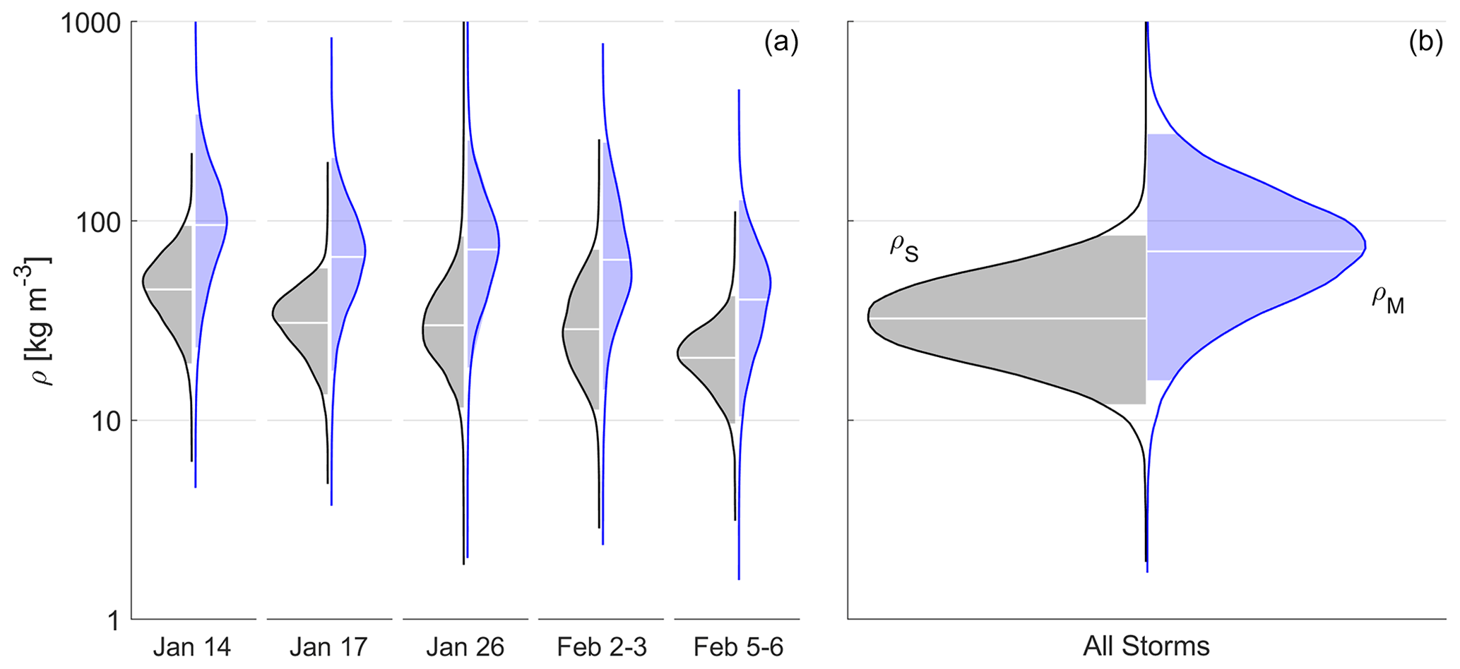
Figure 6 Linear probability density functions of snow density measurements using the spherical volume assumption (gray) and the MASC-adjusted volume (blue) separated into individual storms (a) and for all snowflakes (b). Mean values and ±2σ values are represented by white horizontal lines and the boundary between shading and white space under the tails of the curves.

3.2 Diameter and aspect ratio

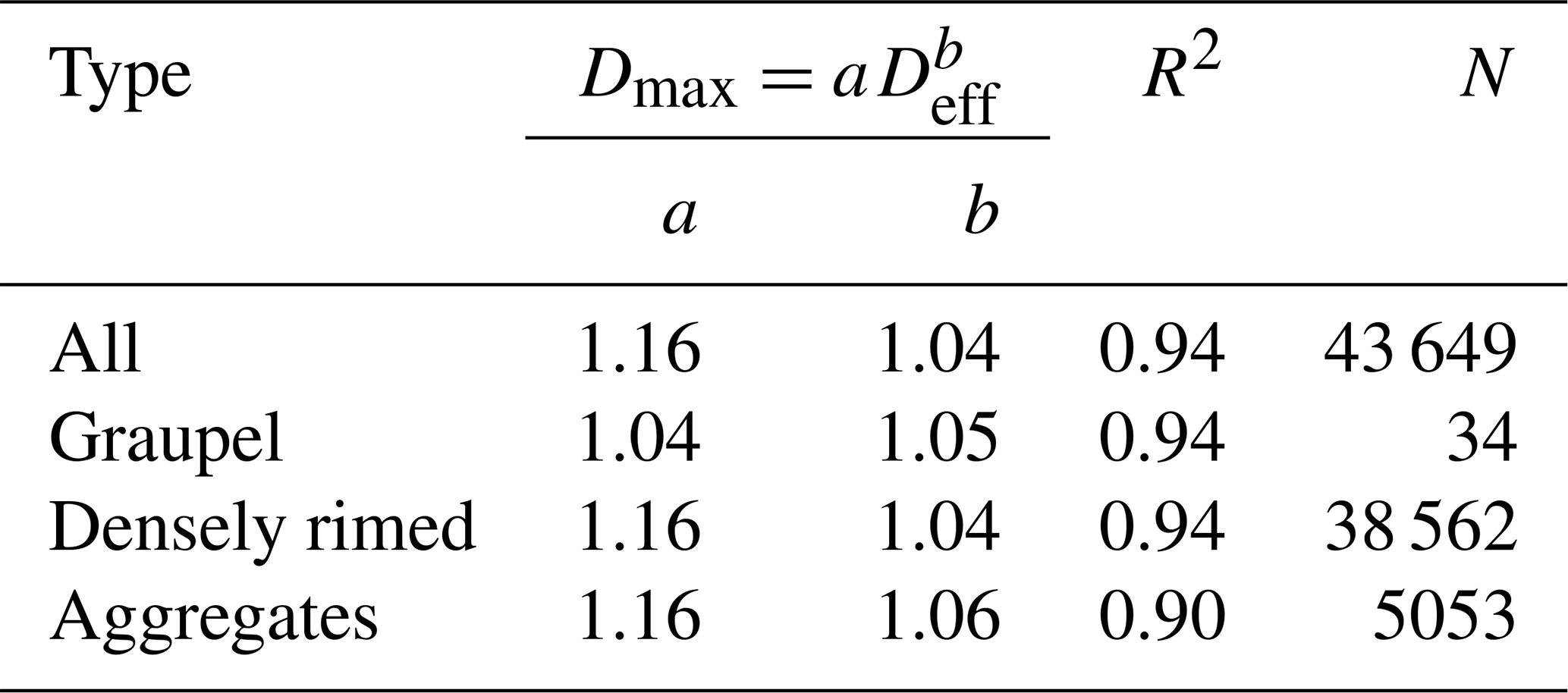
In the following sections, mass–diameter and density–diameter relationships are expressed with respect to D_eff. By way of reference, for the 43 649 snowflakes included in this study that are categorized by type, D_max can be correlated with D_eff through the power-law relationship $D_{\max }=a{D}_{\mathrm{eff}}^b$, with values for a and b summarized in Table 1. In general, the two quantities are highly correlated, and the relationship is nearly linear. For the ensemble taken as a whole, the relationship is $D_{\max }=\mathrm{1.16}{D}_{\mathrm{eff}}^{\mathrm{1.04}}$, with a square correlation coefficient of R²=0.94. The average measured aspect ratios seen by the MASC for aggregates, densely rimed particles, and graupel were 0.64, 0.65, and 0.82 respectively.

Table 1 Relationships between hydrometeor circumscribed and effective diameter.

3.3 Mass–diameter relationships

The mass–diameter relationship for all snowflakes is shown in Fig. 7. The prefactor observed in the mass–diameter relationship is 0.018, which is approximately consistent with the range of values described by Locatelli and Hobbs (1974) for the densely rimed snowflakes (Table 2), comprising 88 % of the snowflakes observed in our study. The exponent 2.52, however, generally exceeds those values obtained by Locatelli and Hobbs (1974) for graupel-like (2.1 to 2.4), densely rimed (2.1 to 2.3), and aggregated (1.4 to 1.9) snow.

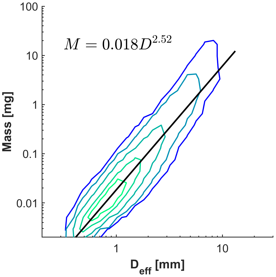
Figure 7 Mass–diameter relationship for all 86 285 snowflakes. Contours shown are for the 25th, 50th, 75th, 90th, and 95th percentiles.

Figure 8 Mass–diameter relationships from the DEID (solid lines) sorted by type according to MASC imagery and compared with fits from Locatelli and Hobbs (1974), dashed lines. Contours are for 50th, 75th, 90th, and 95th percentile bounds.

Snowflakes were selected manually through visual classification using MASC imagery for time periods at least 3 min long where no other snow types were present, defined as aggregates (N=5053), graupel (N=34), and densely rimed (N=38 562). The densely rimed category includes all snowflakes not categorized as graupel or aggregates following Garrett and Yuter (2014). It also includes densely rimed aggregates and partially melted aggregates. Figures 3 and C1–C4 show mostly planar type crystals present, but aggregated needles are frequently seen as well. Graupel occurred frequently, although there was only one 16 min long period that did not exhibit any other type of snow. Mass–diameter relationships $M=a{D}_{\mathrm{eff}}^b$ for graupel, densely rimed snow, and aggregates are compared with those found by (Locatelli and Hobbs, 1974) in Fig. 8 and Table 2. Values of a and b for graupel determined by the DEID (a=0.047 and b=2.73) lie within the ranges observed by Locatelli and Hobbs (1974): $\mathrm{0.042}<a<\mathrm{0.140}$ and $\mathrm{2.6}<b<\mathrm{3.0}$. The quantity of densely rimed and aggregate snowflakes collected by the DEID was roughly 5 orders more numerous than those described by Locatelli and Hobbs (1974). For densely rimed snowflakes, the prefactor a lies within the range observed by Locatelli and Hobbs (1974), and the exponent b is within 11 %. Aggregate snowflakes differ by 12 % in the exponent and by 38 % in the prefactor. In contrast to the findings of Erfani and Mitchell (2017), which state that particle riming changes the prefactor a but not b, here both a and b decrease with increased riming.

Figure 9 illustrates the sensitivity of mass–diameter relationship parameters to particle type and ambient air temperature. Garrett and Yuter (2014) employed the MASC-derived complexity parameter, $\mathit{\chi }=P(\mathrm{1}+<\mathit{\sigma }>)/\left(\mathrm{2}r\right)$, where P is the snowflake perimeter, r is the snowflake radius, and $<\mathit{\sigma }>$ is the intensity variability, to classify snowflakes into three categories: graupel (χ<1.35), densely rimed ($\mathrm{1.35}\le \mathit{\chi }\le \mathrm{1.75}$), and aggregates (χ>1.75). Threshold values of 1.3 and 1.8 have also been previously used (Garrett et al., 2015). Here we adopt threshold values of 1.3 and 1.7. Graupel-like snow is included in the graupel category; the two data points with χ<1.3 include 9506 snowflakes, which are unlikely to be solely graupel due to 1 min averaging of χ and the presence of other snow types observed during graupel events. This category has values of b consistent with the exponent values between 2.1 and 2.4 found by Locatelli and Hobbs (1974). The densely rimed category, however, has exponent values between 2.5 and 2.7, which are higher than those seen by Locatelli and Hobbs (1974), although the difference may be influenced by presence of a large number of partially melted snowflakes that bring the exponent closer to 3. Overall, smaller values of b are obtained as χ exceeds 1.7 and snowflakes transition into aggregates. Notably, the value of b is never lower than 2.

Partially melted snowflakes are excluded favoring more aggregate type snowflakes by restricting analysis to particles that fell when the ambient air temperature was $<-\mathrm{3}$ ^∘C, as represented by blue lines in Fig. 9. There is a clear sensitivity in the mass–diameter relationships to ambient air temperature. For all snowflakes that occurred when the ambient air temperature was <0 ^∘C (N=30 651), the values of a and b are 0.017 and 2.33, respectively, with R²=0.85. For all snowflakes that fell when the ambient air temperature was $<-\mathrm{3}$ ^∘C (N=4630), the corresponding values are 0.015 and 2.12, with R²=0.84.

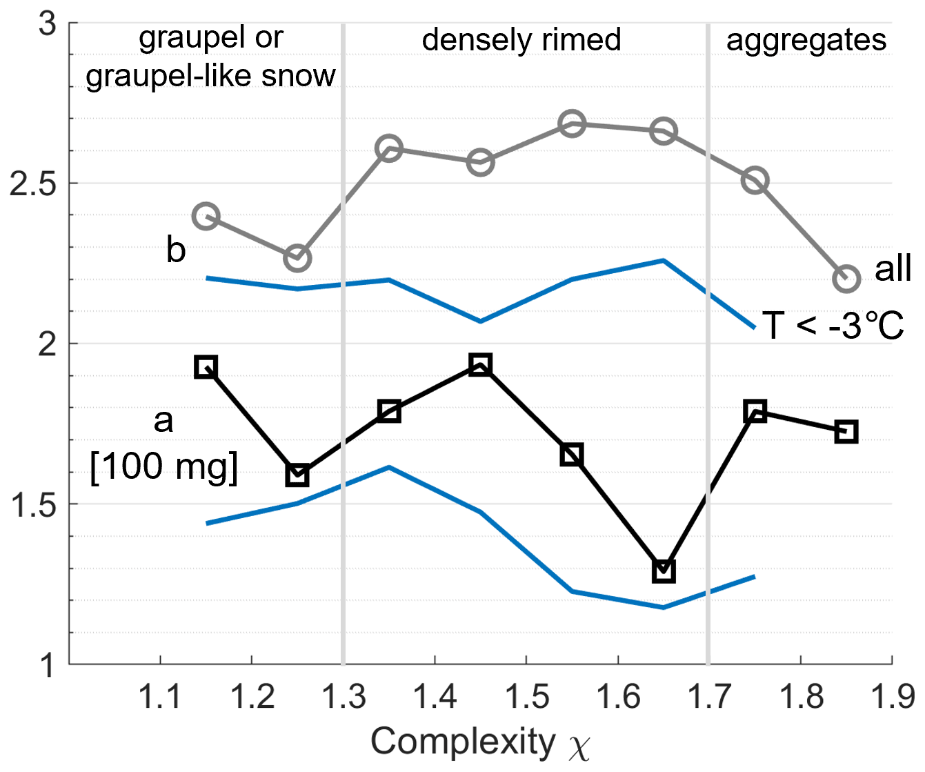
Figure 9 Exponent (gray) and prefactor (black) values in the mass–diameter relationship as binned by 1 min average particle complexity and filtered by ambient temperature (blue line).

Table 2 Mass–diameter relationship comparison by type.

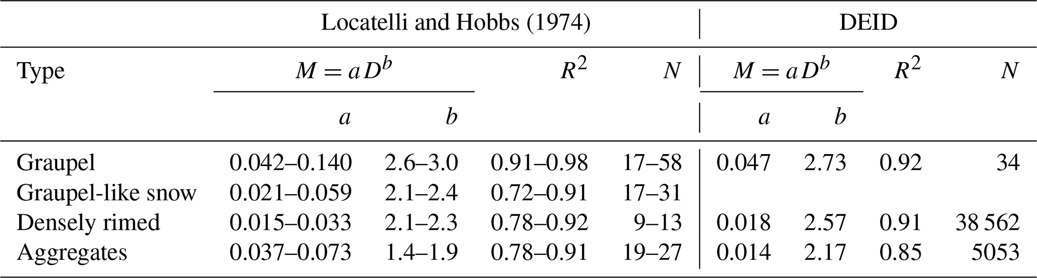
Mass–diameter relationship M=aD^b, where mass is in milligrams and diameter is in millimeters.

3.4 Density–diameter relationship

Density–diameter relationships for all snowflakes in this study are shown in Fig. 10, and a comparison of density–diameter relationships from this work and prior studies is shown in Fig. 11. Using the spherical volume approximation (Fig. 10, left), the measured values for density are rarely greater than 100 kg m⁻³, suggesting a possible underestimate. Using a similar assumption, Muramoto et al. (1995) observed similarly low values of density (Fig. 11). The density–diameter relationships from other studies shown in Fig. 11 include both dry and wet snowflakes and ice particles with densities extending into the 200–300 kg m⁻³ range for the lowest diameters observed.

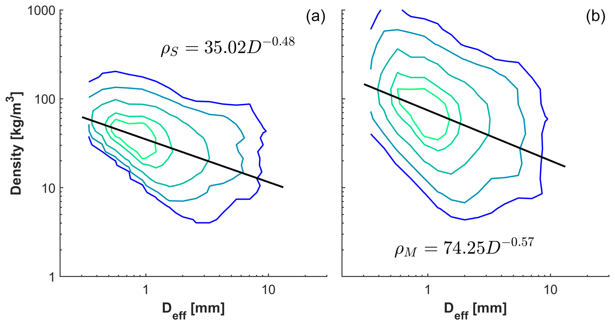
Figure 10 Density–diameter relationships for spherical (a) and MASC-adjusted (b) volume for all snowflakes. Contours shown are for the 25th, 50th, 75th, 90th, and 95th percentiles.

More refined density calculations supplemented by MASC data are shown in Fig. 10, right, and include high values near the density of bulk water, as would be expected for wet snowflakes that have partially melted before reaching the hotplate. The prefactors a are 35.02 and 74.25 for the spherical and MASC-adjusted density respectively, and the exponents b are −0.48 and −0.57. The values of a and b were also obtained when filtering snowflakes by temperature to exclude partially melted snowflakes (T<0 ^∘C) and to reflect primarily aggregate snowflakes ($T<-$3 ^∘C), and they are shown in Table 3.

Table 3 Density–diameter relationship comparison by ambient air temperature.

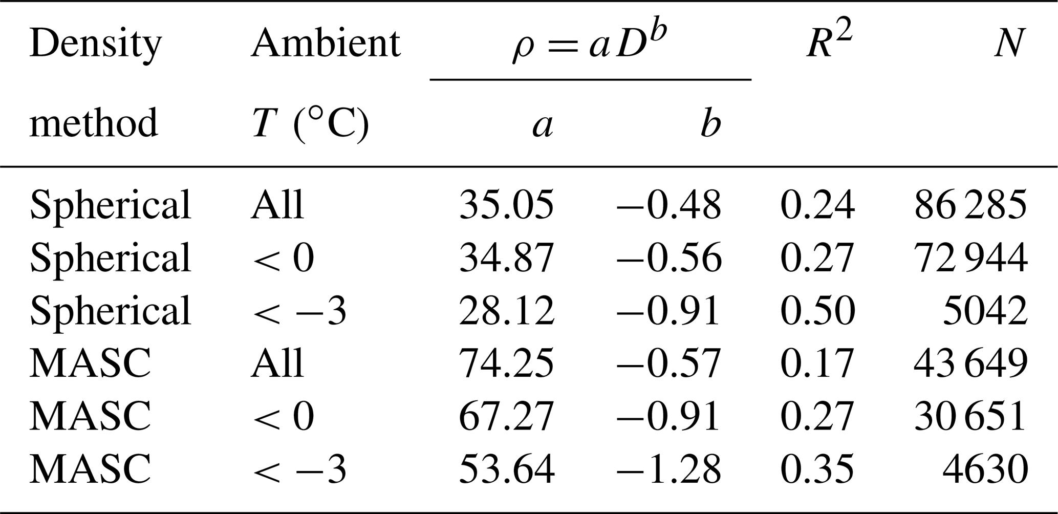
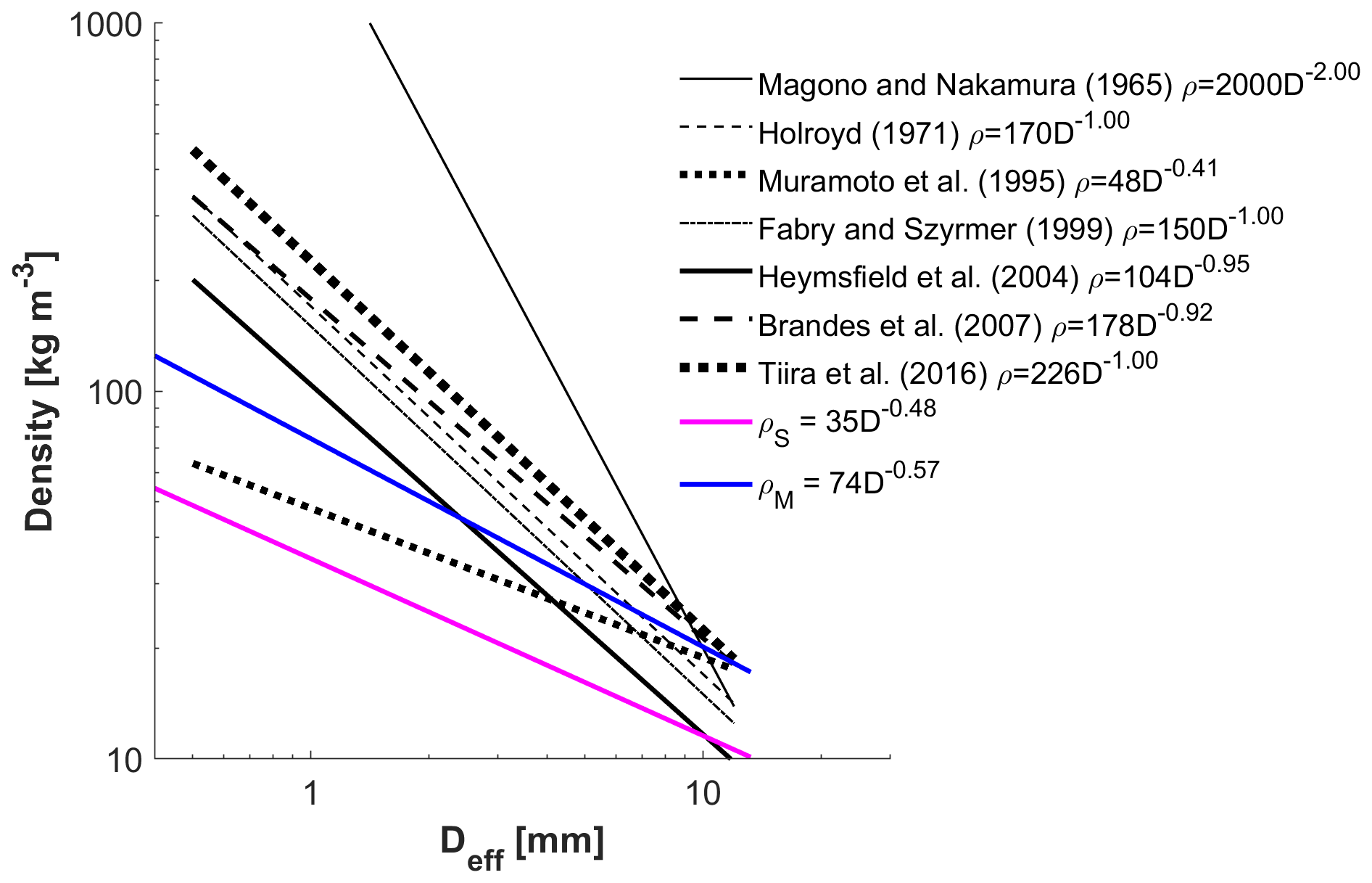
Figure 11 Density–diameter relationships from previous studies and those obtained here using the spherical density method (magenta) and MASC-adjusted density method (blue).

4 Discussion

A notable difference between the mass–diameter relationships from our study versus those described previously by Locatelli and Hobbs (1974) lies in fitted exponents for both densely rimed and aggregate type snowflakes. In the earlier study these ranged from 2.1 to 2.3 for densely rimed and 1.4 to 1.9 for aggregates, while our results point to exponents of 2.57 and 2.17. An added implication of the larger exponents is that the masses of very small aggregates with diameters less than 1 mm are generally smaller than have previously been reported (Fig. 8). While the MASC-adjusted density–diameter relationships align closely with several previous studies (Fig. 11) for particle sizes larger than approximately 5 mm diameter, much lower values of density tend to be observed at smaller particle sizes. Where the exponents described in previous studies (Holroyd, 1971; Fabry and Szyrmer, 1999; Heymsfield, 2003; Brandes et al., 2007; Tiira et al., 2016) are close to −1, those from our study are approximately −0.5, suggesting a weaker dependence of density on particle size than is generally assumed, especially at ambient air temperatures near 0 ^∘C. However, by excluding higher temperatures near freezing to omit partially melted snowflakes, the exponents more closely approach −1. The average density of all hydrometeors using the spherical volume assumption is 38 and 90 kg m⁻³ using the MASC-adjusted volume. For comparison, the density of snowfall on the ground at a high-elevation location in the Wasatch Mountains in Utah is typically less than 100 kg m⁻³ (Alcott and Steenburgh, 2010), a location where mode snowflake diameters lie between 1 and 2 mm (Garrett and Yuter, 2014).

5 Summary

We describe measurements of the mass and density of individual frozen hydrometeors obtained using a new instrument, the Differential Emissivity Imaging Disdrometer. Power-law mass–diameter relationships obtained by the DEID derived from 86 285 measured particles agree well with widely used relationships published by Locatelli and Hobbs (1974), which were based on a much more limited dataset. The exception is that snowflakes measured by the DEID have exponents higher by between 12 % and 38 %. To obtain hydrometeor density from the measured mass, estimates of volume are required. Here, a simple spherical approximation for particle volume based on the particle equivalent diameter seen by a thermal camera viewing the heated plate led to density estimates approximately a factor of 2 lower than those using a more refined calculation that incorporated concurrent MASC measurements of the particle aspect ratio. For the subset of DEID measurements that included coincident MASC imagery totaling 43 649 hydrometeors, the resulting density–diameter relationships suggest substantially lower densities of particles smaller than 5 mm than has been observed in most prior studies. It may be that existing bulk microphysical parameterizations in numerical weather models tend to underestimate the masses of large frozen hydrometeors while overestimating those of smaller hydrometeors. If true, any revision could have possible implications for forecasts of snow water deposition in mountain reservoirs. Future anticipated refinements to the DEID particle volume algorithm at a wider range of locations may help further refine estimates of hydrometeor density.

Appendix A: Hotplate calibration

The constant K_d, which includes the specific heat capacity, equivalent latent heat, and the plate's thickness and thermal conductivity, was calibrated experimentally for the DEID aluminum plate (Singh et al., 2021). The plate was roughened with 600-grit (P1200) sandpaper to allow for droplet spreading and more rapid evaporation of water during calibration experiments. Water drops of known masses were evaporated on the plate to determine the calibrated coefficient. Combining the constants in Eq. (1) yields

$$\begin{array}{}\text{(A1)}& (c_p\mathrm{\Delta }{T}_{\mathrm{ev}}+L_{\mathrm{v}})M={\displaystyle \frac{K}{H}}\underset{\mathrm{0}}{\overset{t}{\int }}A\left(t\right)(T_{\mathrm{p}}-T_{\mathrm{w}}(t\left)\right)\mathrm{d}t,\end{array}$$

where M is a known mass of water. A constant is determined that includes the thermal conductivity and the thickness of the hotplate using droplets of known mass $M=\mathrm{2}\pm \mathrm{0.2}\times {\mathrm{10}}^{-\mathrm{5}}$ kg:

$$\begin{array}{}\text{(A2)}& {\displaystyle \frac{K}{H}}={\displaystyle \frac{M(c_{p,\mathrm{w}}\mathrm{\Delta }{T}_{\mathrm{ev}}+L_{\mathrm{v}})}{{\int }_{\mathrm{0}}^{t}A\left(t\right)T_{\mathrm{p}}-T_{\mathrm{w}}\left(t\right)\mathrm{d}t}},\end{array}$$

where ${\int }_{\mathrm{0}}^t{T}_{\mathrm{p}}-T_{\mathrm{w}}\left(t\right)A\left(t\right)\mathrm{d}t$ was determined from DEID measurements, $c_{p,\mathrm{w}}=\mathrm{4.28}\times {\mathrm{10}}^{\mathrm{3}}$ J K⁻¹ kg⁻¹ is the specific heat of water at constant pressure, ΔT_ev=100 K, and $L_{\mathrm{v}}=\mathrm{2.26}\times {\mathrm{10}}^{\mathrm{6}}$ J kg⁻¹ is the latent heat of vaporization. Determined through 10 trials, $K/H=\mathrm{4.1}\pm \mathrm{0.1603}\times {\mathrm{10}}^{\mathrm{3}}$ kg s⁻³ K⁻¹.

Including the latent and specific heat required to evaporate liquid water and ice, respectively, the derived values of K_d for liquid and ice are then

$$\begin{array}{ll}{\displaystyle }{K}_{\mathrm{d},\mathrm{l}}=& {\displaystyle \frac{K/H}{(c_{p,\mathrm{w}}\mathrm{\Delta }{T}_{\mathrm{ev}}+L_{\mathrm{v}})}}={\displaystyle \frac{\mathrm{4.1}\times {\mathrm{10}}^{\mathrm{3}}}{\mathrm{2.67}\times {\mathrm{10}}^{\mathrm{6}}}}=\\ \text{(A3)}& {\displaystyle }& {\displaystyle }\mathrm{1.54}\times {\mathrm{10}}^{-\mathrm{3}}\left[{\displaystyle \frac{\text{kg}}{{\text{s\hspace{0.17em}K\hspace{0.17em}m}}^{\mathrm{2}}}}\right],{\displaystyle }{K}_{\mathrm{d},\mathrm{i}}=& {\displaystyle \frac{K/H}{(c_{p,\mathrm{w}}\mathrm{\Delta }{T}_{\mathrm{ev}}+L_{\mathrm{v}}+c_{p,\mathrm{i}}\mathrm{\Delta }{T}_m+L_{\mathrm{f}})}}=\\ \text{(A4)}& {\displaystyle }& {\displaystyle \frac{\mathrm{4.1}\times {\mathrm{10}}^{\mathrm{3}}}{\mathrm{3.03}\times {\mathrm{10}}^{\mathrm{6}}}}=\mathrm{1.35}\times {\mathrm{10}}^{-\mathrm{3}}\left[{\displaystyle \frac{\text{kg}}{{\text{s\hspace{0.17em}K\hspace{0.17em}m}}^{\mathrm{2}}}}\right],\end{array}$$

where $c_{p,\mathrm{i}}=\mathrm{2.10}\times {\mathrm{10}}^{\mathrm{3}}$ J K⁻¹ kg⁻¹ is the specific heat of ice at constant pressure and the latent heat of fusion $L_{\mathrm{f}}=\mathrm{3.34}\times {\mathrm{10}}^{\mathrm{5}}$ J kg⁻¹. The equation for mass becomes $M=K_{\mathrm{d}}{\int }_{\mathrm{0}}^{t}A\left(t\right)(T_{\mathrm{p}}-T_{\mathrm{w}}(t\left)\right)\mathrm{d}t$.

Experiments comparing mass calculations using ${\int }_{\mathrm{0}}^{t}A\left(t\right)T_{\mathrm{p}}-T_{\mathrm{w}}\left(t\right)\mathrm{d}t$ and $\mathrm{\Delta }T{\int }_{\mathrm{0}}^{t}A\mathrm{d}t$, where $\mathrm{\Delta }T=T_{\mathrm{p}}-T_{\mathrm{w}}\left(t\right)$ is the mean value per particle, showed that the latter is a sufficient approximation and the equation for mass may then be expressed as

$$\begin{array}{}\text{(A5)}& M=K_{\mathrm{d}}\mathrm{\Delta }T\underset{\mathrm{0}}{\overset{t}{\int }}A\left(t\right)\mathrm{d}t.\end{array}$$

Appendix B: Image processing

The MATLAB Image Processing Toolbox was used to extract data from the thermal camera to determine the physical properties of individual melted hydrometeors. Experimentally relevant parameters include the hotplate temperature T_p, the sampling frequency of the thermal camera f_s, the physical width of each pixel in the camera imagery p, and the sampling area of the hotplate A_hot. Each thermal camera image was converted to both grayscale and binary format. Three-dimensional volumetric regions, “voxels”, in a product space of hydrometeor area on the DEID plate and time during the duration of the melting of each particle were evaluated to yield the particle mass through Eq. (A5), as illustrated in Figs. B1–B5.

For the sake of processing, all partial voxel objects that bordered the edge of the 3D sampling area were removed for individual particle calculations. A filtering threshold was used to remove small particles with fewer than three pixel data points in any dimension.

The temperature difference between the hotplate and water ($\mathrm{\Delta }T=T_{\mathrm{p}}-T_{\mathrm{w}}\left(t\right)$) is based on the mean pixel intensity of the particle during its lifetime on the hotplate. The mean pixel intensity I_mean is converted to ΔT through the linear transformation ($(T_{\mathrm{p}}-T_{\mathrm{w}}(t\left)\right)\approx \mathrm{\Delta }T=T_{\mathrm{p}}(\mathrm{255}-I_{\mathrm{mean}})/\mathrm{256}$).

The integrated cross-sectional area of the particle during its evaporation time on the hotplate is given by $V_t=\int A\left(t\right)\mathrm{d}t$. The effective diameter D_eff is calculated from the point in time associated with the maximum recorded cross-sectional area of the particle A_max according to $D_{\mathrm{eff}}=\sqrt{\frac{\mathrm{4}}{\mathit{\pi }}{A}_{\max }}$. The evaporation time of each particle is calculated by generating a bounding box, or the smallest box that contains the 3D region containing V_t, where the circumscribed diameter D_max is the maximum in the area dimension and the evaporation time t_evap is the maximum in the time dimension.

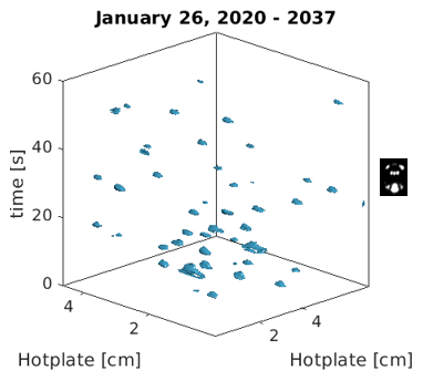
Figure B1 Volumetric rendering of melting rain hydrometeors in area on the DEID plate and in time such that each isosurface represents a rain drop frozen at a point in time.

Figure B2 As for Fig. B1 but for partly melted hydrometeors.

Figure B3 As for Fig. B1 but for aggregate snow.

Figure B4 As for Fig. B1 but for densely rimed aggregate snow.

Figure B5 As for Fig. B1 but for a mixture of densely rimed and aggregate snow.

Appendix C: MASC snowflake imagery

MASC imagery of frozen hydrometeors was catalogued for each snow event described in this article with representative particles shown in Figs. C1 to C4.

Figure C1 MASC snowflake imagery for 14 January 2020.

Figure C2 MASC snowflake imagery for 17 January 2020.

Figure C3 MASC snowflake imagery for 26 January 2020.

Figure C4 MASC imagery for 2 to 3 February 2020.