Supersaturation, buoyancy, and deep convection dynamics

Motivated by recent discussions concerning differences of convective dynamics in polluted and pristine environments, the so-called convective invigoration in particular, this paper provides an analysis of factors affecting convective updraft buoyancy, such as the in-cloud supersaturation, condensate and precipitation loading, and entrainment. We use the deep convective period from simulations of daytime convection development over land discussed in our previous publications. An entraining parcel framework is used in the theoretical analysis. We show that for the specific case considered here, finite (positive) supersaturation noticeably reduces pseudo-adiabatic parcel buoyancy and cumulative convective available potential energy (cCAPE) in the lower troposphere. This comes from keeping a small fraction of the water vapor in a supersaturated state and thus reducing the latent heating. Such a lower-tropospheric impact is comparable to the effects of condensate loading and entrainment in the idealized parcel framework. For the entire tropospheric depth, loading and entrainment have a much more significant impact on the total CAPE. For the cloud model results, we compare ensemble simulations applying either a bulk microphysics scheme with saturation adjustment or a more comprehensive double-moment scheme with supersaturation prediction. We compare deep convective updraft velocities, buoyancies, and supersaturations from all ensembles. In agreement with the parcel analysis, the saturation-adjustment scheme provides noticeably stronger updrafts in the lower troposphere. For the simulations predicting supersaturation, there are small differences between pristine and polluted conditions below the freezing level that are difficult to explain by standard analysis of the in-cloud buoyancy components. By applying the piggybacking technique, we show that the lower-tropospheric buoyancy differences between pristine and polluted simulations come from a combination of temperature (i.e., latent heating) and condensate loading differences that work together to make polluted buoyancies and updraft velocities slightly larger when compared to their pristine analogues. Overall, the effects are rather small and contradict previous claims of a significant invigoration of deep convection in polluted environments.

1 Introduction

In the presence of gravity, density differences within a fluid give rise to the Archimedean buoyancy force that drives fluid vertical motions. The magnitude of the buoyancy force per unit mass – the buoyancy for short – is expressed as $g(\mathit{\rho }-{\mathit{\rho }}_{\mathrm{o}})/{\mathit{\rho }}_{\mathrm{o}}$, where g is the acceleration of gravity, and ρ and ρ_o are the densities of the volume of fluid under consideration and the reference (environmental) fluid density, respectively. The buoyancy of cloudy air depends on the air temperature and pressure, water vapor content, and mass of all cloud and precipitation particles within the volume. It is typically expressed through the so-called density temperature or density potential temperature (see Sect. 4.3 in Emanuel, 1994). For the case of the anelastic model applied in numerical simulations discussed in this paper¹, the buoyancy B is defined as follows (see Eq. 5 in Grabowski and Smolarkiewicz, 2002):

$$\begin{array}{}\text{(1)}& B=g\left[(\mathrm{\Theta }-{\mathrm{\Theta }}^{\mathrm{e}})/{\mathrm{\Theta }}_{\mathrm{0}}+\mathit{\epsilon }\left(q_{\mathrm{v}}-q_{\mathrm{v}}^{\mathrm{e}}\right)-q\right],\end{array}$$

where Θ and q_v are the potential temperature and water vapor mixing ratios, Θ^e is the hydrostatically balanced environmental potential temperature profile, $q_{\mathrm{v}}^{\mathrm{e}}$ is the corresponding environmental water vapor mixing ratio profile, Θ₀ is the base state anelastic potential temperature profile, q is the sum of all condensate and precipitation liquid and ice mixing ratios, and $\mathit{\epsilon }=R_{\mathrm{v}}/R_{\mathrm{d}}-\mathrm{1}\approx \mathrm{0.6}$ (R_v and R_d are the gas constants for water vapor and dry air, respectively). The base-state and environmental profiles are typically derived from the initial sounding used in the simulations. The three terms in the square bracket on the right-hand side of Eq. (1) are referred to as the temperature, virtual, and mass-loading terms.

There are two key processes that affect cloudy air buoyancy. The first is the phase change in the water substance that modifies the air temperature and can alter the virtual and mass-loading terms. For instance, the condensation of Δ = 1 g kg⁻¹ of water vapor mixing ratio changes the air temperature by ∼ $L_{\mathrm{v}}/c_{\mathrm{p}}\mathrm{\Delta }$ or about 2.5 K and contributes ∼ 0.01g to the cloud buoyancy (L_v≈ 2.5 × 10⁶ J kg⁻¹ is the latent heat of condensation, c_p≈ 1005 $\mathrm{J}{\mathrm{kg}}^{-\mathrm{1}}{\mathrm{K}}^{-\mathrm{1}}$ is the specific heat of air at constant pressure). Condensation reduces the virtual term by about 0.0006g and increases the loading term by 0.001g. Hence, the buoyancy increase due to temperature change is about an order of magnitude larger than the other terms. For the liquid to ice phase change, the freezing of Δ = 1 g kg⁻¹ of liquid water mixing ratio changes the air temperature by $L_{\mathrm{f}}/c_{\mathrm{p}}\mathrm{\Delta }$ or about 0.3 K and contributes ∼ 0.001g to the buoyancy with no effect on virtual and mass-loading terms (L_f≈ 3 × 10⁵ J kg⁻¹ is the latent heat of freezing). The second key process affecting cloudy air buoyancy concerns precipitation. Precipitation allows the condensate q in Eq. (1) to leave the volume (the condensate off-loading) and thus increases the volume buoyancy. For instance, the converting of Δ = 1 g kg⁻¹ of cloud condensate (cloud water or ice) into precipitation (rain or snow) and off-loading it increases the volume buoyancy by ∼ 0.001g, that is, similar to the impact of freezing it. The similar contributions to the buoyancy of the latent heat of freezing and of the mass loading are the crux of the argument against the hypothesized convection invigoration in polluted environments. The invigoration argument alleges that carrying the liquid water across the 0 ^∘C level (rather than converting it to rain and off-loading below the freezing level) and freezing it aloft leads to stronger upper-tropospheric updrafts in the polluted environments; see the discussion in Sect. 2a of Grabowski and Morrison (2020, GM20 hereafter, and references therein) and the exchange between Fan and Khain (2021) and Grabowski and Morrison (2021). Precipitation can also fall from above into the volume under consideration and reduce its buoyancy.

There is also a more subtle effect related to the presence of the supersaturation in natural clouds.² Positive supersaturation reduces the latent heating when compared to the situation with no supersaturation because some water vapor is left in the supersaturated state. This leads to a decrease in the cloud buoyancy because latent heating dominates the impact on the buoyancy as illustrated above. The impact of the latent heating difference between pristine and polluted clouds is referred to in Fan et al. (2018) as “warm-phase invigoration”. Grabowski and Jarecka (2015) derived the density potential temperature difference between situations with finite and zero supersaturations. The difference is approximately a linear function of the supersaturation and depends on the temperature and pressure. In the lower troposphere, supersaturation of 0.01 (i.e., 1 %) reduces the density temperature by about 0.1 K (see Fig. 1 in Grabowski and Jarecka, 2015), that is, by ∼ 0.0003g. However, if the supersaturation ratio is much larger, say 0.1 (i.e., 10 %), the impact becomes comparable to the loading of a few grams per kilogram of the cloud or precipitation mixing ratio. The impact gets smaller in the middle and upper troposphere because the same supersaturation as in the lower troposphere translates into a smaller absolute difference in the condensation rate between the finite and zero supersaturation with lower temperature (cf. Fig. 2 in Grabowski and Morrison, 2017).

Finally, buoyancy is strongly affected by entrainment of environmental air and cloud dilution. Entrainment has been argued to affect mean cloud properties from the early days of cloud dynamics based on theory and observation (e.g., Stommel, 1947; Warner, 1955). For shallow convection, entrainment typically leads to buoyancy reversal, that is, replacing the positive buoyancy from condensation inside an undiluted updraft with a negative buoyancy resulting from the cloud water evaporation as a result of entrainment (see Grabowski, 1993, and references therein). For deep-scattered (unorganized) convection, high-resolution (large eddy simulation (LES)-type) simulations have shown considerable dilution of updraft core properties (e.g., Kuang and Bretherton, 2006; del Genio and Wu, 2010; Peters et al., 2020) despite having generally smaller fractional entrainment rates than shallow cumulus (de Rooy et al., 2013). Fractional entrainment rates (as well as environmental relative humidity) control the dilution of core buoyancy and hence strongly influence updraft velocities (de Rooy and Siebesma, 2010; Morrison, 2017; Peters et al., 2020). In this way, entrainment rate also has a dominant influence on the shallow-to-deep transition and ultimately the height attained by moist updrafts (e.g., Khairoutdinov and Randall, 2006; Kuang and Bretherton, 2006; Morrison et al., 2021). Although the critical impact of entrainment on cumulus updraft properties is well accepted, to our knowledge there has been no work analyzing how entrainment impacts the buoyancy changes driven by finite supersaturations.

A traditional cloud physics view is that supersaturations in natural clouds are small, say a fraction of 1 %, except near the cloud base when activation of cloud condensation nuclei (CCN) takes place (e.g., Pruppacher and Klett, 1997). Supersaturations cannot be measured directly but can be estimated by assuming a balance between supersaturation source due to local updraft and supersaturation sink due to growth of cloud droplets. The supersaturation estimated in this way is referred to as the quasi-equilibrium supersaturation (Squires, 1952). The quasi-equilibrium supersaturation provides an accurate estimate of the in-cloud supersaturation as long as the phase relaxation time of the droplet population (that depends on the droplet mean radius and concentration) is short compared to the timescales characterizing changes in the droplet population and the cloud updraft (see, for instance, the appendix in Grabowski and Morrison, 2021). Estimation of the quasi-equilibrium supersaturation in relatively weak convective clouds featuring gentle updrafts and insignificant precipitation agrees with the traditional view (e.g., Politovich and Cooper, 1988). Measurements of the local updraft strength and droplet spectral characteristics in deep convective clouds with strong updrafts and significant precipitation are difficult using an instrumented aircraft because of flight safety. Prabha et al. (2011, Fig. 9 therein) document observations from pre-monsoon and monsoon deep convective clouds over the Indian subcontinent with updrafts up to about 10 m s⁻¹ and corresponding quasi-equilibrium supersaturations up to several percent. The condensation rate inside a rising adiabatic parcel featuring the quasi-equilibrium supersaturation depends on the vertical velocity alone and is independent of the droplet concentration and radius (see Sect. 2a in GM20). Thus, differences in the condensation rate between polluted and pristine clouds can only occur by an updraft change (resulting from a difference in the cloud buoyancy), a change in entrainment and mixing, or by supersaturation being different from its quasi-equilibrium value.

From the early days of warm (ice-free) cloud modeling, a typical approach has been to assume that clouds always maintain saturation (e.g., Morton, 1957; Ogura, 1963; Orville, 1965; Soong and Ogura, 1973). For dynamic cloud models, such a computationally efficient approach for calculating cloud condensation and evaporation is referred to as saturation adjustment and has been applied in both compressible (e.g., Klemp and Wilhelmson, 1978) and anelastic (e.g., Clark, 1979; Lipps and Hemler, 1982) models. With the advent of more complicated warm-rain microphysics schemes, such as the double-moment (Morrison and Grabowski, 2007, and references therein) and spectral (bin) microphysics (e.g., Kogan, 1991; Feingold et al., 1996) that allow estimation of the droplet concentration and mean radius, such schemes began predicting in-cloud supersaturation. Khain and Lynn (2009), Lebo and Seinfeld (2011), and Lebo et al. (2012) compared supercell splitting simulations applying bulk saturation-adjustment schemes and saturation-prediction bin microphysics. Khain and Lynn (2009) applied the bin microphysics together with the Thompson scheme (Thompson et al., 2004) and showed almost a doubling of the maximum vertical velocity for the bulk scheme (35 for bin versus 65 m s⁻¹ for bulk; see Fig. 2 there) and doubling of the surface rain accumulation (see Fig. 5 there). Such differences are unlikely because of the simulated supersaturation alone and require different explanations, for instance, different organization of deep convective cells simulated by the two schemes as suggested by maps of the surface rain accumulations. Lebo and Seinfeld (2011) applied a similar simulation framework to compare supercell simulations using their bin microphysics scheme with those using the Morrison double-moment bulk scheme employing saturation adjustment (Morrison et al., 2005). Rainfall accumulations over the simulated 6 h period were about twice as large in the bulk scheme as in the bin scheme, and there were significant differences in the surface rain accumulation maps (e.g., see Figs. 3, 4, and 5). These seem to agree with the Khain and Lynn (2009) differences. Profiles of the mean convective core updrafts in Lebo and Seinfeld (2011) differ significantly as well, with stronger updrafts in the bulk scheme (see Figs. 7 and 13 there). Using the same framework and different modifications of the Morrison bulk scheme, Lebo et al. (2012) show values of the supersaturations in their simulations in excess of 10 % (see Fig. 13 there). Simulations of shallow to deep convection transition based on observations over the Amazon discussed in Grabowski and Morrison (2016, see Figs. 9 and 13 there; and 2020, see Fig. 10 there) also show that the supersaturations in deep convective cores below the freezing level can reach up to 10 % with several percent supersaturation differences between pristine and polluted conditions. Zhang et al. (2021) discuss simulations of deep convection over the Houston area by applying the Morrison scheme as in Lebo and Seinfeld (2011), together with Khain et al. (2004) bin microphysics. They show similar convective organization in simulations applying the two schemes and argue that bin results are in a better agreement with observations. Although the differences between results from simulations applying the two schemes are relatively small, there is some convective invigoration as represented by stronger updraft velocities and larger surface precipitation in the polluted case.

The purpose of the current study is to analyze contributions to the updraft buoyancy by applying theory (Sect. 3) and results of numerical simulations (Sect. 4). The impact of finite supersaturation on general aspects of convective dynamics (e.g., on convective available potential energy – CAPE) has not been investigated previously. Grabowski and Morrison (2016, 2020) argue that the impact of pollution on convective dynamics as simulated by a double-moment microphysics scheme predicting in-cloud supersaturation comes from the supersaturation differences between pristine and polluted conditions. This is because the impact is limited to the lower troposphere (i.e., below the melting level) and it is absent in simulations applying saturation adjustment (Grabowski, 2015; see also Grabowski and Morrison, 2021). However, the buoyancy differences have not been discussed in detail, for instance, contributions from the entrainment to pristine–polluted differences and the impact of condensate loading. Theoretical analysis and additional analysis of simulations presented in our previous papers is the focus of the current paper.

2 Cloud model simulations

2.1 The model setup and microphysics schemes

Model simulations analyzed here were previously discussed in Grabowski (2015; G15 hereinafter), Grabowski and Morrison (2020; GM20), and Grabowski and Morrison (2021). A short description of the simulations is given below, with details provided in the above publications.

G15 and GM20 apply a daytime convective development modeling case from Grabowski et al. (2006). The 12 h long simulations, an extension of 6 h simulations in Grabowski et al. (2006), start with the observed morning sounding and are driven by the surface sensible and latent heat fluxes. The fluxes strongly increase with the daytime surface insolation, reach a mid-day maximum, and decrease to zero during the 10th hour of the simulation (see Fig. 1 in G15). The morning increase in the surface fluxes leads to the development of a well-mixed convective boundary layer, followed by the formation of shallow convective clouds, transition from shallow to deep convection around local noon, and only remnants of upper-tropospheric anvils present at the end of the simulations. Because convective development is forced only by prescribed surface heat fluxes, the same in all simulations, the differences in simulated convection come from different microphysics representations. The simulations feature a doubly periodic 50 km by 50 km horizontal domain with 400 m horizontal grid length. In the vertical, a stretched grid with 81 levels is used with about 10 (20) levels in the lowest 1 (4) km, reaching up to 24 km height. Overall, the horizontal resolution is relatively low, making the simulations only marginally LESs, especially early in the simulations when the boundary layer is relatively shallow. However, as mentioned in G15 (Sect. 2a therein) applying such a grid provides results broadly consistent with the high-resolution benchmark simulations reported in Grabowski et al. (2006). Results reported here seem also consistent with truly LESs reported in Kurowski et al. (2018) and in Grabowski and Prein (2019). A small ensemble of simulations (see details below) is run for each case, with ensemble members generated by different sets of random numbers applied during the initialization and during model run as detailed in Grabowski et al. (2006).

G15 applied a relatively simple single-moment bulk microphysics scheme, referred to as IAB (ice A and B; Grabowski, 1999). IAB includes a simple warm-rain parameterization with a prescribed droplet concentration, 100 versus 1000 per cc to mimic pristine (PRI) versus polluted (POL) conditions. The assumed droplet concentration affects conversion from cloud water to rain. IAB uses saturation adjustment to calculate cloud water condensation and evaporation. The ice parameterization is simple and is linked only indirectly to the assumed droplet concentration. Two classes of the ice mixing ratio are considered: slowly falling ice A and fast-falling ice B. Ice A represents unrimed or lightly rimed ice particles whose spectral characteristics are assumed to follow aircraft observations in tropical upper-tropospheric anvil clouds. Ice B, on the other hand, represents heavily rimed ice particles (e.g., graupel) which occur in the vicinity of convective towers. Besides G15, the IAB scheme was successfully applied in deep convection simulations described in Varble et al. (2014), Fridlind et al. (2012), and Mrowiec et al. (2012). For more details, see the brief discussion in Sect. 2b of G15 or a full description in Grabowski (1999).

The GM20 double-moment (2MOM) bulk microphysics scheme is more comprehensive. Droplet concentration is predicted together with the in-cloud supersaturation. CCN activation together with cloud droplet growth and evaporation are calculated explicitly from the predicted supersaturation instead of relying on saturation adjustment (Morrison and Grabowski, 2007, 2008a). The warm-rain component predicts both number and mass mixing ratios for cloud water and rain (i.e., four Eulerian variables). The double-moment three-variable ice microphysics of Morrison and Grabowski (2008b) predicts the number mixing ratio of ice particles and two mass mixing ratios that represent the ice mass grown by the diffusion of water vapor and by riming. This allows for a smooth transition from unrimed ice particles to heavily rimed particles (i.e., graupel) instead of artificially dividing ice particles into cloud ice, snow, and graupel categories that requires the introduction of unphysical conversion rates. Primary ice initiation occurs through several processes, including deposition/condensation freezing, heterogeneous freezing of cloud droplets and rain drops, contact freezing of cloud droplets, and homogeneous freezing of all droplets and drops for temperatures below −40 ^∘C. The key feature of the scheme is the close link between ice and warm-rain processes and the connection between droplet and ice number mixing ratios in particular. See Sect. 2a in Grabowski and Morrison (2016) for a more extensive discussion or a full description of the scheme in Morrison and Grabowski (2007, 2008a, b). The simulations discussed in GM20 include a pristine case (PRIS) that features a single CCN mode with the number mixing ratio of 100 mg⁻¹ and a polluted case with an additional mode of smaller CCN with 500 mg⁻¹ number mixing ratio, referred to as ADCN. Overall, having two different microphysics parameterizations allows results to be compared with not only saturation adjustment and supersaturation prediction but also significantly different microphysics parameterizations.

Table 1 Ensembles of the dynamic model simulations discussed in this paper. All simulations apply the same computational domain, horizontal grid length, and vertical grid structure. G06 is Grabowski et al. (2006). IAB is the microphysics scheme discussed in Grabowski (1999) that features single-moment warm-rain and ice microphysics with prescribed cloud droplet concentrations and excludes water supersaturation by applying saturation adjustment. 2MOM is the double-moment microphysics described in Morrison and Grabowski (2007, 2008a, b) with mass and number mixing ratios for liquid condensate (i.e., four variables) and three ice variables (one number mixing ratio and two mass mixing ratios). The 2MOM scheme predicts in-cloud supersaturation and allows water supersaturation. See text for more details.

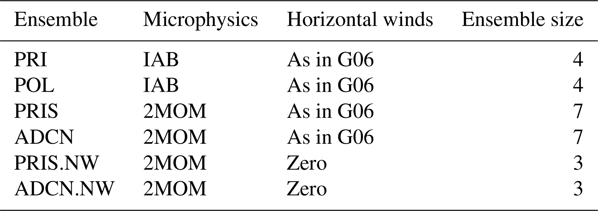
Results from the following ensemble simulations will be discussed. Four ensembles, two for IAB (PRI and POL) and two for 2MOM (PRIS and ADCN) relax the simulated mean horizontal winds to prescribed profiles as in Grabowski et al. (2006), with four ensemble members for IAB's PRI and four for IAB's POL, as well as seven ensemble members for 2MOM's PRIS and seven for 2MOM's ADCN. Horizontal winds in Grabowski et al. (2006) feature significant shear (cf. Fig. 9 in GM20), and because of that we also consider the 2MOM no-horizontal-wind simulations in GM20 as in Wu et al. (2009) and Böing et al. (2012). These two three-member ensembles are referred to as PRIS.NW and ADCN.NW (NW for “no wind”). The reason for different numbers of ensemble members will become apparent in the discussion of model results (see Fig. 2). The simulations are summarized in Table 1.

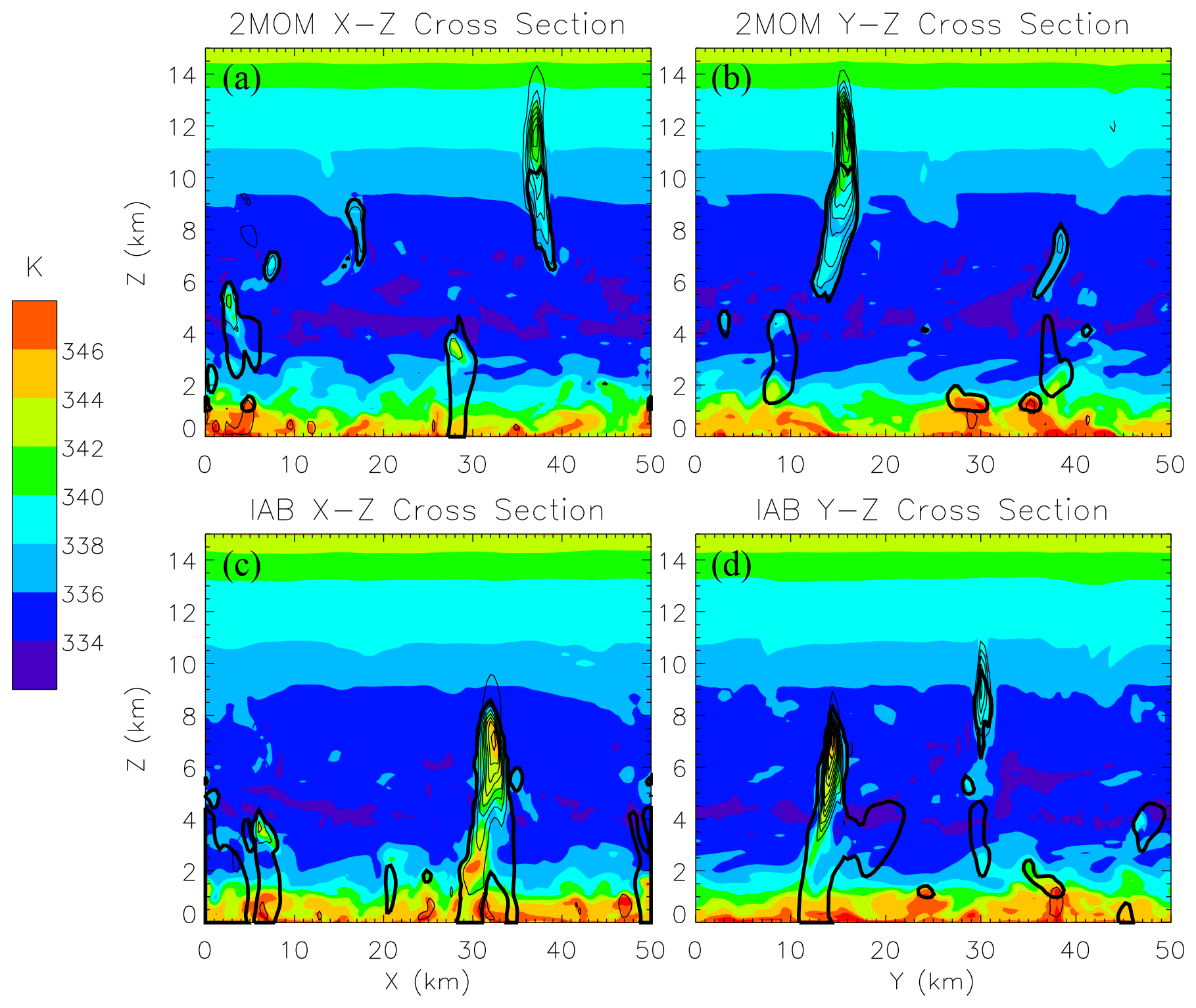
Figure 1 Cross sections (x–z in a and c; y–z in b and d) though cloud simulations at 360 min from (a, b) 2MOM and (c, d) IAB randomly selected ensemble members. Colors represent the equivalent potential temperature, calculated here as the moist static energy divided by c_p. The thick contour shows total condensate (cloud and precipitation) of 0.1 g kg⁻¹. Sold thin contours show vertical velocity starting with 1 m s⁻¹ and contour interval of 3 m s⁻¹.

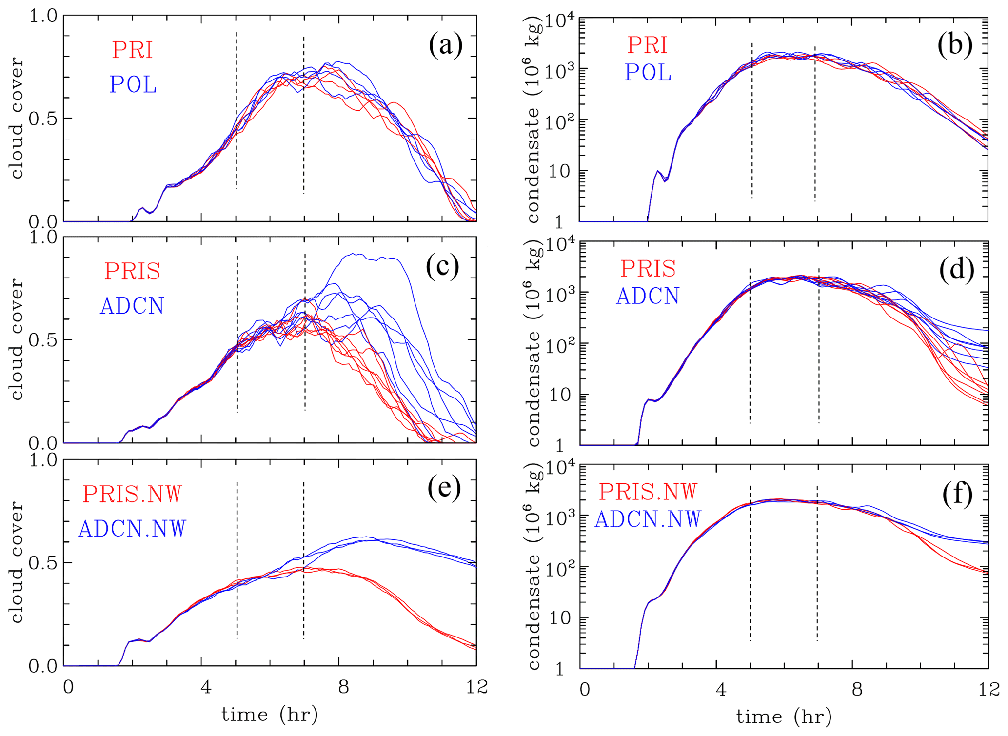
Figure 2 Evolution of (a, c, e) cloud cover and (b, d, f) total mass of cloud and precipitation inside the computational domain in (a, b) PRI and POL IAB ensembles, (c, d) PRIS and ADCN 2MOM ensembles, and (e, f) PRIS.NW and ADCN.NW 2MOM ensembles. Dashed vertical lines show the 6th and 7th hour period for which analyses are completed.

2.2 Illustration of macroscopic cloud field characteristics

To highlight key similarities and differences between the IAB and 2MOM simulations, Figs. 1 and 2 show vertical cross-section snapshots from randomly selected ensemble members at hour 6 (i.e., 360 min) and evolutions of the cloud cover and total condensed water mass for the entire simulation length. The vertical cross sections in the X (east–west) and Y (north–south) directions are taken at the location of domain-maximum vertical velocity. At 360 min, the 2MOM simulation in Fig. 1 features a very deep convective tower that seems detached from the lower levels in the east–west and north–south cross sections, but this simply reflects the effects of shear causing the cloud to “lean” along the diagonal. There are also a few shallow clouds. In the IAB simulation snapshot, the cloud containing the domain-maximum vertical velocity at hour 6 is shallower but growing rapidly. The cloud still has traces of lower-tropospheric moist static energy as shown by orange and red colors. The mean pattern of the moist static energy is similar between the two simulations. In Fig. 2, the cloud cover in the left panels is defined as the fraction of columns with at least one grid volume featuring total condensate larger than 0.1 g kg⁻¹, with the total condensate including all cloud and precipitation mixing ratios. Figure 2b, d, and f show the evolution of the total condensate mass inside the computational domain. Total condensate increases due to the condensation and deposition and decreases due to evaporation, sublimation, and precipitation reaching the surface. Overall, Fig. 2 shows that IAB and 2MOM ensembles feature similar cloud field evolutions despite significant differences in the microphysics parameterizations. The figure documents small differences in IAB's PRI and POL simulations, as already discussed in G15. In contrast, the 2MOM simulations show large differences between PRIS and ADCN in the second half of the simulations. These differences are argued in GM20 (and also in Grabowski and Morrison, 2016) to come from the microphysical impact of pristine versus polluted CCN conditions on the upper-tropospheric anvils. In a nutshell, higher cloud droplet concentrations in the polluted case result in higher ice crystal concentrations aloft, and this leads to smaller mean ice crystal sizes, lower sedimentation velocities, and thus longer residence times. Figure 2 also illustrates different variability between ensemble members depending on the presence or absence of the mean large-scale flow, which informed our ensemble size selection. The vertical dotted lines in Fig. 2 mark the period of hours 6 and 7 (300 to 420 min), with the strongest deep convection that is used for the analyses presented in subsequent sections.

3 Theoretical considerations: idealized parcel calculations

We use domain-averaged temperature and water vapor mixing ratio profiles for the 6th and 7th simulation hours (i.e., averaged between 300 to 420 min and over all ensemble members) in a rising parcel analysis. The change in a generic thermodynamic quantity Φ with height for a rising parcel is given by (similar to Betts, 1973, neglecting detrainment)

$$\begin{array}{}\text{(2)}& \mathrm{d}\mathrm{\Phi }/\mathrm{d}z=-\mathit{\epsilon }(\mathrm{\Phi }-{\mathrm{\Phi }}^{\mathrm{e}})+S_{\mathrm{\Phi }},\end{array}$$

where ε is the fractional entrainment rate, S_Φ is the source/sink of Φ owing to cooling by expansion and water phase changes, and Φ^e is the corresponding environmental value taken from the thermodynamic profile used in the analysis (i.e., the domain average potential temperature and water vapor for the 6th and 7th hour; the environment cloud water mixing ratio is assumed zero). Considering Φ as a moist conserved or nearly conserved quantity such as total water mixing ratio q_t (water vapor plus condensed water, neglecting removal by sedimentation) or equivalent potential temperature Θ_e, the source/sink term S_Φ is (or is close to) zero. Using the base state pressure profile and the simplified form of Θ_e used for the analysis later (see Sect. 4b), which is analogous to moist static energy, it is equivalent to solve Eq. (2) for Θ_e and q_t and diagnose Θ, water vapor mixing ratio q_v, and condensate mixing ratio q needed for the buoyancy from Θ_e and q_t, or solve Eq. (2) directly for Θ, q_v, and q. We chose the latter approach.³ As shown in Sect. 4b, solving Eq. (2) assuming a constant ε can reproduce reasonably well updraft Θ_e profiles from the simulations. Thus, the simple parcel approach given by Eq. (2) can capture bulk behavior of the simulated updrafts.

The derived parcel Θ, q_v, and q are subsequently applied to obtain the buoyancy profile using Eq. (1) and then to calculate the cumulative convective available potential energy (cCAPE) at height z defined as

$$\begin{array}{}\text{(3)}& \text{cCAPE}\left(z\right)=\underset{\mathrm{0}}{\overset{z}{\int }}max(\mathrm{0},B)\mathrm{d}z.\end{array}$$

Buoyancy is calculated assuming an air parcel with the initial temperature and water vapor values taken as the mean in the lowest 500 m of the atmosphere and starting at 500 m height. The mean low-level temperature and moisture values change little between the IAB and 2MOM ensembles (less than 0.1 K for the temperature and less than 0.1 g kg⁻¹ for the water vapor); such changes have a small impact on the results (e.g., ∼ 100 J kg⁻¹ or less than 5 % for the pseudo-adiabatic CAPE). Starting parcel calculations with the surface temperature and water vapor values changes specific results documented in this section, but the relative impacts of the finite supersaturation, loading, and entrainment remain similar (not shown). Profiles from the 2MOM PRIS ensemble are used in the analysis presented below. The total CAPE is equal to cCAPE at the updraft equilibrium level, that is, at the level where the updraft buoyancy changes aloft from positive into negative.

The pseudo-adiabatic parcel analysis excludes the condensate term q in Eq. (1); that is, the analysis assumes that the condensate is converted to precipitation and falls out with no impact on the parcel buoyancy. In the traditional parcel analysis, the rising parcel is assumed to maintain water saturation at all heights above the lifting condensation level (LCL), in other words, applying saturation adjustment. However, one can assume non-vanishing supersaturation S, say assuming S=0, 0.05, and 0.1 throughout the entire troposphere (i.e., 0, 5, and 10 % supersaturation). For comparison, we also include parcel analysis with the buoyancy that includes a fraction of the condensate loading f of $\mathrm{1}/\mathrm{3}$, $\mathrm{2}/\mathrm{3}$, and all condensate (f=1) in Eq. (1) at each level; thus, we implicitly assume a fraction 1−f of the condensate is removed by conversion to precipitation followed by sedimentation. Finally, we also consider the impact of parcel dilution assuming three different fractional entrainment rates: ε = 0.05, 0.1, and 0.3 km⁻¹. This range of ε is broadly consistent with bulk fractional entrainment rates derived from previous modeling studies for deep convection (e.g., Kuang and Bretherton, 2006; Del Genio and Wu, 2010; De Rooy et al., 2013) and derived from the simulations in Sect. 4b. Assuming a classical entrainment formulation of ε $\sim \mathrm{0.2}/R$, where R is the parcel radius (e.g., de Rooy et al., 2013), gives R = 4, 2, and 0.6 km for the three ε values selected.

Figure 3 Profiles of (a, c, e) cumulative CAPE (cCAPE) and (b, d, f) buoyancy from parcel analysis using mean temperature and humidity profiles from the lowest 500 m of 2MOM PRIS simulation averaged over the 6th and 7th hours. (a, b) Pseudo-adiabatic parcel calculations with different supersaturations. (c, d) Parcel calculations with different fractions of the condensate included in parcel buoyancy. (e, f) Entraining parcel calculations with different fractional entrainment rates.

Table 2 Results from parcel simulations. The table shows CAPE together with cCAPE and buoyancy at 4 and 9 km height. The first three rows show results from the pseudo-adiabatic parcel analysis assuming saturation adjustments of S=0 %, 5 %, and 10 % throughout the atmosphere. The middle three rows show results from parcel calculations that assume saturation adjustment and include $\mathrm{1}/\mathrm{3}$, $\mathrm{2}/\mathrm{3}$, and full condensate loading. The bottom three rows show results of entraining parcel calculations assuming saturation adjustment and no loading with three entrainment rates: 0.05, 0.1, and 0.3 km⁻¹. The initial temperature and water vapor values in the parcel are taken as averages in the lowest 500 m and over hours 6 and 7 from the 2MOM PRIS ensemble.

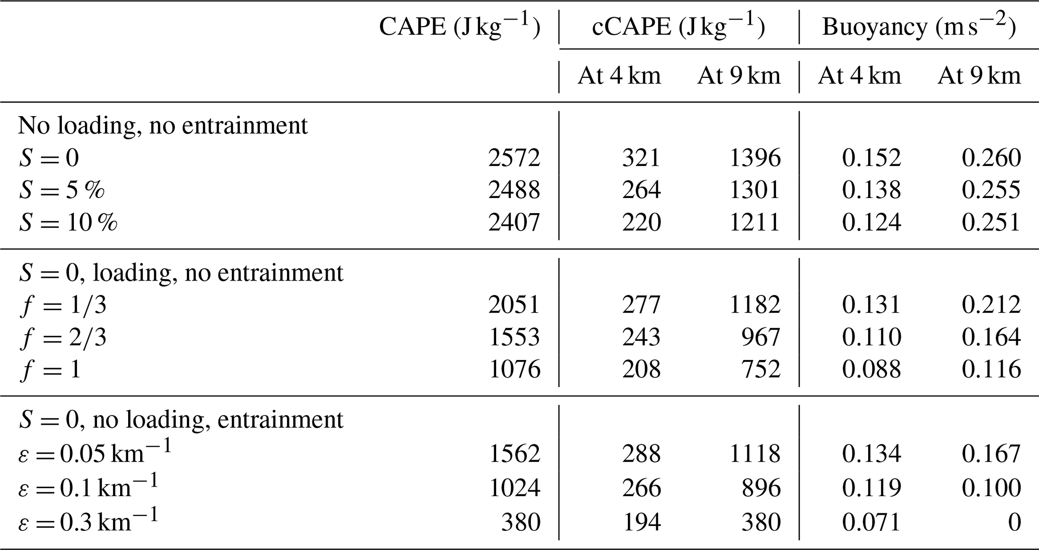
Figure 3 shows profiles of cCAPE and buoyancy for the parcel analysis with numerical values at heights of 4 and 9 km presented in Table 2. For the pseudo-adiabatic parcel (Fig. 3a and b), limiting the parcel to water saturation (S = 0) provides the largest buoyancy, at least in the lower and middle troposphere, which is consistent with the theoretical analysis and simulations of Grabowski and Jarecka (2015) and Grabowski and Morrison (2017). Retaining supersaturated conditions in the finite-supersaturation pseudo-adiabatic parcel leads to a small but noticeable reduction in buoyancy, cCAPE, and CAPE (see Table 2). It also allows for additional latent heating above 11 km, but the upper-tropospheric buoyancy difference has little impact on the total CAPE because CAPE is dominated by the lower- and middle-tropospheric buoyancy differences. The pseudo-adiabatic buoyancy increases up to about 8 km height and decreases in the upper troposphere, with the total CAPE reaching values around 2500 J kg⁻¹. Calculating a theoretical updraft vertical velocity as $w=\sqrt{\mathrm{2}\text{cCAPE}}$, obtained by vertically integrating the parcel vertical velocity equation neglecting perturbation pressure forcing and momentum mixing, gives values around 25 m s⁻¹ for S=0 and around 21 m s⁻¹ for S = 10 % at 4 km. At 9 km, these values are around 53 m s⁻¹ for S=0 and around 49 m s⁻¹ for S = 10 %. These differences are relatively small but non-negligible. Updraft vertical velocities simulated by the dynamic model (see the next section) are 2 to 3 times smaller presumably because of entrainment, the missing loading term in the pseudo-adiabatic parcel analysis, and excluding perturbation pressure forcing in the parcel model, which all (in general) limit the theoretical updraft strength below its equilibrium level.

Including condensate loading in the parcel buoyancy has a significant impact. Using all condensate in the parcel buoyancy is arguably appropriate just above the cloud base before the condensate is reduced by precipitation fallout. However, it is questionable in the middle and upper troposphere because it implies over 10 g kg⁻¹ of cloud condensate, a clearly unrealistic value (this will be illustrated by the analysis later in the paper). Nevertheless, even a third of the cloud condensate notably reduces parcel buoyancy, cCAPE, and CAPE. The theoretical updraft strength at 4 km changes from about 24 m s⁻¹ for $f=\mathrm{1}/\mathrm{3}$ to about 20 m s⁻¹ for f=1; at 9 km these values are 49 and about 39 m s⁻¹, respectively. Entrainment has a large impact as well, with the smallest fractional entrainment rate tested (0.05 km⁻¹) reducing cCAPE by about 10 % at 4 km and 20 % at 9 km compared to an undilute parcel and the total CAPE by about 25 %. The theoretical updraft w at 4 km changes from about 25 m s⁻¹ for ε = 0.05 km⁻¹ to about 20 m s⁻¹ for ε = 0.3 km⁻¹, similar to the impact of including condensate loading. At 9 km these values for ε of 0.05 and 0.3 km⁻¹ are 47 and 39 m s⁻¹, respectively. The largest fractional entrainment rate tested, ε = 0.3 km⁻¹, gives an equilibrium level in the mid-troposphere (∼ 8 km) compared to > 12 km in the other tests (Fig. 3f). The lower equilibrium height with greater ε is expected and is consistent with previous theoretical (Morrison et al., 2021) and cloud modeling (e.g., Kuang and Bretherton, 2006) studies. Finally, we point out that there is almost no impact of entrainment or loading on absolute differences in cCAPE resulting from changes in S between 0 % and 10 % (not shown). This can be understood by the fact that changes in parcel temperature from entrainment are small relative to the parcel temperature itself (∼ 1 % or less). Thus, changes in parcel temperature owing to changes in S can be well approximated as being independent of entrainment. Because the magnitude of cCAPE decreases from entrainment, the relative change in cCAPE from finite S increases with greater entrainment. Similarly, changes in q owing to finite S (up to 10 %) are small relative to q itself. Thus, including loading has little impact on absolute changes to cCAPE from finite S, although relative changes to cCAPE increase.

In summary, the theoretical analysis presented in this section shows that finite supersaturation (up to 10 %) has a non-negligible impact on convective dynamics. However, the impact is relatively small overall when compared to the effects of condensate loading and entrainment. Moreover, including loading or entrainment has almost no impact on absolute differences in cCAPE resulting from changes in S (but relative differences in cCAPE increase since both entrainment and loading act to decrease cCAPE). Larger changes in cCAPE and w might be possible if ε or f are different in polluted compared to pristine conditions. These factors are considered further in dynamic model simulations discussed in the next section.

4 Results of dynamic simulations

4.1 Entrainment and its impact on updraft velocity

To characterize the impact of entrainment on the buoyancy and updraft velocity, we apply an equivalent potential temperature Θ_e defined here as the moist static energy divided by c_p​​​​​​​:

$$\begin{array}{}\text{(4)}& {\mathrm{\Theta }}_{\mathrm{e}}=T+g/c_{\mathrm{p}}z+L_{\mathrm{v}}/c_{\mathrm{p}}{q}_{\mathrm{v}},\end{array}$$

where T, z, and q_v are the temperature, height, and water vapor mixing ratio, and L_v and c_p are the latent heat of condensation and air-specific heat at constant pressure. For a rising adiabatic or pseudo-adiabatic parcel with no ice processes, the equivalent potential temperature Θ_e defined in Eq. (4) is an invariant for the anelastic model and the moist precipitating thermodynamics applied in both saturation adjustment (IAB) and saturation prediction (2MOM) ensembles. Moreover, regardless of the condensate amount carried by the cloudy air, mixing between the cloudy air parcel and subsaturated cloud-free environmental parcel results in the equivalent potential temperature which is a linear combination of the relative mass contributions of the two parcels Θ_e.

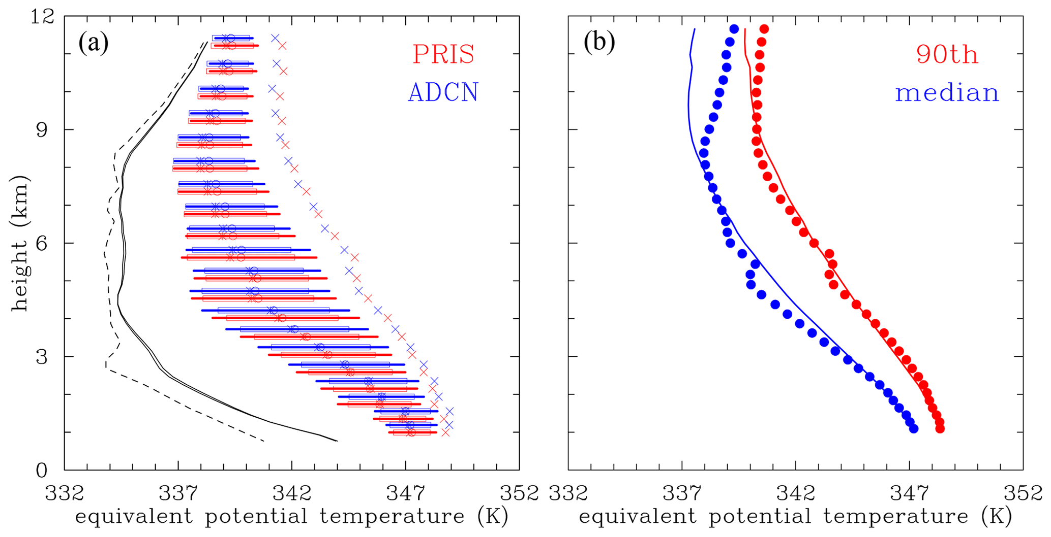
Figure 4 (a) Comparison of equivalent potential temperature statistics during the 6th and 7th hours from GM20 PRIS (red) and ADCN (blue) simulations. Asterisks represent median values, thick lines mark the range between the 10th and 90th percentiles, circles show the mean values, and “x” symbols to the right of the boxes represent means of the range between the 90th percentile and the maximum. Boxes represent the range between the mean and plus and minus 1 standard deviation. Only in-cloud points with vertical velocity larger than 1 m s⁻¹ and total condensate larger than 1 g kg⁻¹ are included in the statistics. The dashed black line is the equivalent potential temperature profile calculated from the initial sounding. The two solid lines are the equivalent potential temperature profiles calculated from the mean temperature and moisture profiles averaged over the 6th and 7th hours from PRIS and ADCN ensemble simulations. (b) Comparison between model and entraining parcel results. Dots are median (blue) and 90th percentile (red) values from the PRIS results in (a). Lines are profiles of the equivalent potential temperature derived from the entraining parcel with the constant entrainment rate that minimizes the difference between the parcel and either the median or the 90th percentile profile from the model between 1 and 10 km. See text for more details.

Figure 4a shows the equivalent potential temperature Θ_e statistics for in-cloud points with updraft velocity larger than 1 m s⁻¹ and total condensate larger than 1 g kg⁻¹ for all members of GM20's PRIS and ADCN ensembles during the 6th and 7th simulation hours. The dashed line shows the Θ_e profile of the initial sounding, and solid lines show Θ_e profiles of the mean (domain- and time-averaged) temperature and moisture during hours 6 and 7. The difference between the dashed and solid lines represents the impact of surface latent and sensible heat fluxes combined with the vertical transport throughout the column. Arguably, radiative cooling during the day and especially throughout the night, not considered in the simulations, would be needed to bring the dashed and solid lines closer to each other if the simulations were extended to several diurnal cycles (i.e., approaching convective–radiative quasi-equilibrium).

Undiluted ascent from the cloud base would correspond to a vertical line in Fig. 4a, so there is almost always some cloud dilution by entrainment of environmental air. The figure is similar to higher-resolution simulations of this case in Khairoutdinov and Randall (2006); see Figs. 11 and 12 there. This is in contrast to results presented in Varble et al. (2014, see Fig. 16 there) that show very little dilution across the entire troposphere for an ensemble of mesoscale convective system simulations possibly because of the organized nature of convection in their simulations compared to the scattered convection here and in Khairoutdinov and Randall (2006). Dilution corresponding to the mean Θ_e and the minimum dilution (i.e., the mean of the 90th percentile to the maximum range of Θ_e) increases with height as expected; that is, the deviation from the cloud-base Θ_e increases as one moves away from the cloud base. There seems to be a small impact of the microphysics on entrainment dynamics between 3 and 5 km, with slightly smaller mean values of Θ_e for ADCN compared to PRIS. Such a difference may come from small but systematic differences in the mixing proportions between cloud and environmental air in ADCN and PRIS. Plots for the no-wind GM20 ensembles (PRIS.NW and ADCN.NW) are similar, including the small difference between PRIS.NW and ADCN.NW (not shown). Plots for IAB are also similar, although there is no difference between PRI and POL, arguably because saturation adjustment limits differences in latent heating and cooling that impact entrainment dynamics. The latter is consistent with high-resolution simulations in Grabowski and Jarecka (2015). Finally, a kink of the mean and median values (better seen in Fig. 4b discussed below) near 5 km likely comes from Θ_e changes due to ice processes, particularly melting.

Linking directly to the theoretical analysis in Sect. 3, we use profiles of updraft Θ_e from the simulations to estimate constant-in-height fractional entrainment rate ε using our entraining parcel model. This is done by vertically integrating Eq. (2) for Φ=Θ_e between about 1 km (near the level of free convection) and 10 km, using Θ_e from the simulations as a lower boundary condition. ε is estimated by finding the value that minimizes the root-mean-square difference between profiles of Θ_e obtained by solving Eq. (2) and from the simulations. Note that this simple approach estimates a bulk ε value obtained by assuming that entrained properties of air are equal to those of the average environment for hours 6 and 7. This is different from direct entrainment calculations based on the mass fluxes across cloud updraft boundaries (e.g., Romps, 2010; Dawe and Austin, 2013). Direct calculations of ε are generally larger than bulk estimates by up to about a factor of 2 (Romps, 2010). For simplicity, and because we are concerned primarily with updraft dilution as opposed to entrainment per se, we use the bulk approach. Two different Θ_e profiles from the simulations are used to estimate ε: the median and 90th percentile Θ_e. This gives ε for “typical” updrafts, as well as relatively undiluted updrafts (or updraft regions). The best fit ε are ∼ 0.20 km⁻¹ for median Θ_e and 0.13 km⁻¹ for 90th percentile Θ_e. These are similar to previous bulk estimates for deep convection (e.g., Kuang and Bretherton, 2006; Del Genio and Wu, 2010; De Rooy et al., 2013). Figure 4b compares the median and 90th percentile of the dynamic model Θ_e distributions with entraining parcel calculations assuming those best fits. In general, the Θ_e profiles from solving Eq. (2) with these ε values reasonably reproduce the simulated profiles with root-mean-square differences of ∼ 0.8 and 0.4 K for median and 90th percentile Θ_e, respectively. Larger differences in the upper troposphere can be explained by a smaller entrainment rate that allows those cloudy volumes to be present there in the first place, as well as the impact of ice microphysics on Θ_e which is neglected in the parcel calculations. A key result is that best-fit ε values are almost the same for pristine and polluted simulations: 0.203 and 0.206 km⁻¹ for PRIS and ADCN for median Θ_e and 0.131 and 0.127 km⁻¹ for PRIS and ADCN for 90th percentile Θ_e. Thus, in these simulations microphysical differences from polluted versus pristine conditions appear to have little impact on overall entrainment behavior. The small differences in Θ_e between ADCN and PRIS seen in Fig. 4 at mid-levels (∼ 3 to 5 km) evidently have little impact on bulk entrainment differences considering the entire profile between 1 and 10 km.

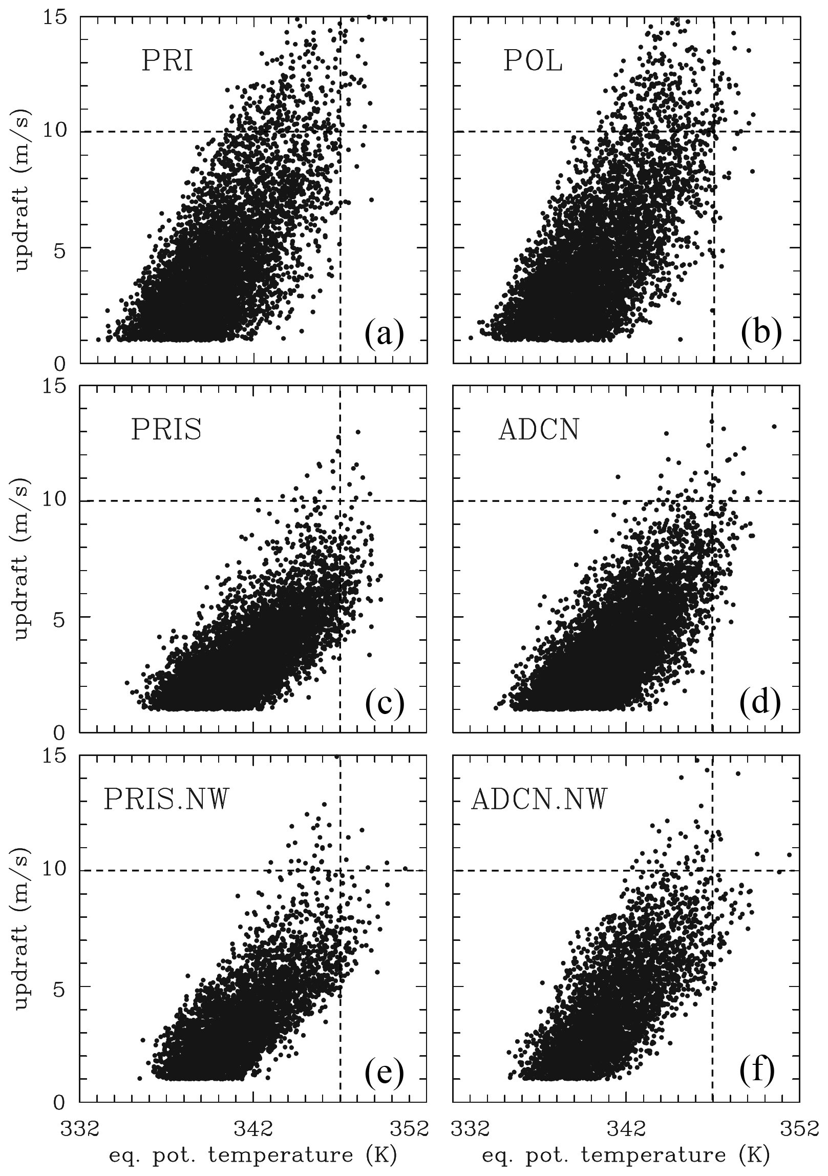
Figure 5 Updraft versus Θ_e for four IAB simulations (PRI and POL; a and b), three 2MOM simulations (randomly selected from seven members for PRIS and ADCN ensembles; c and d), and three 2MOM simulations (from PRIS.NW and ADCN.NW ensembles; e and f). Data at 4 km height for hours 6 and 7 in grid volumes with updraft larger than 1 m s⁻¹ and total condensate larger than 1 g kg⁻¹. Dashed horizontal and vertical lines show values of 10 m s⁻¹ and 347 K to better expose differences discussed in the text.

Figure 5 shows scatterplots of the equivalent potential temperature versus vertical air velocity at a height of 4 km during hours 6 and 7 for all IAB and 2MOM ensemble members and for grid volumes with w larger than 1 m s⁻¹ and total condensate larger than 1 g kg⁻¹. On average, updraft strength increases with Θ_e, but there is a significant scatter. The highest Θ_e for all ensembles is close to the cloud base Θ_e (∼ 250 K as shown in Fig. 4). The saturation-adjustment simulations using IAB, PRI, and POL feature the strongest updrafts, and there is no difference between them except for different flow realizations. In contrast, ADCN and ADCN.NW have stronger updrafts when compared to PRIS and PRIS.NW, but the differences are relatively small, most evident in the difference in the number of points in the range of 5 to 10 m s⁻¹. For that range, the mean updraft in IAB ensembles is 6.87 m s⁻¹ for PRI and 6.91 m s⁻¹ for POL, arguably a statistically insignificant difference. For 2MOM ensembles, the differences are larger, $\mathrm{6.26}/\mathrm{6.53}$ m s⁻¹ for PRIS/ADCN and $\mathrm{6.25}/\mathrm{6.62}$ m s⁻¹ for PRIS.NW/ADCN.NW.

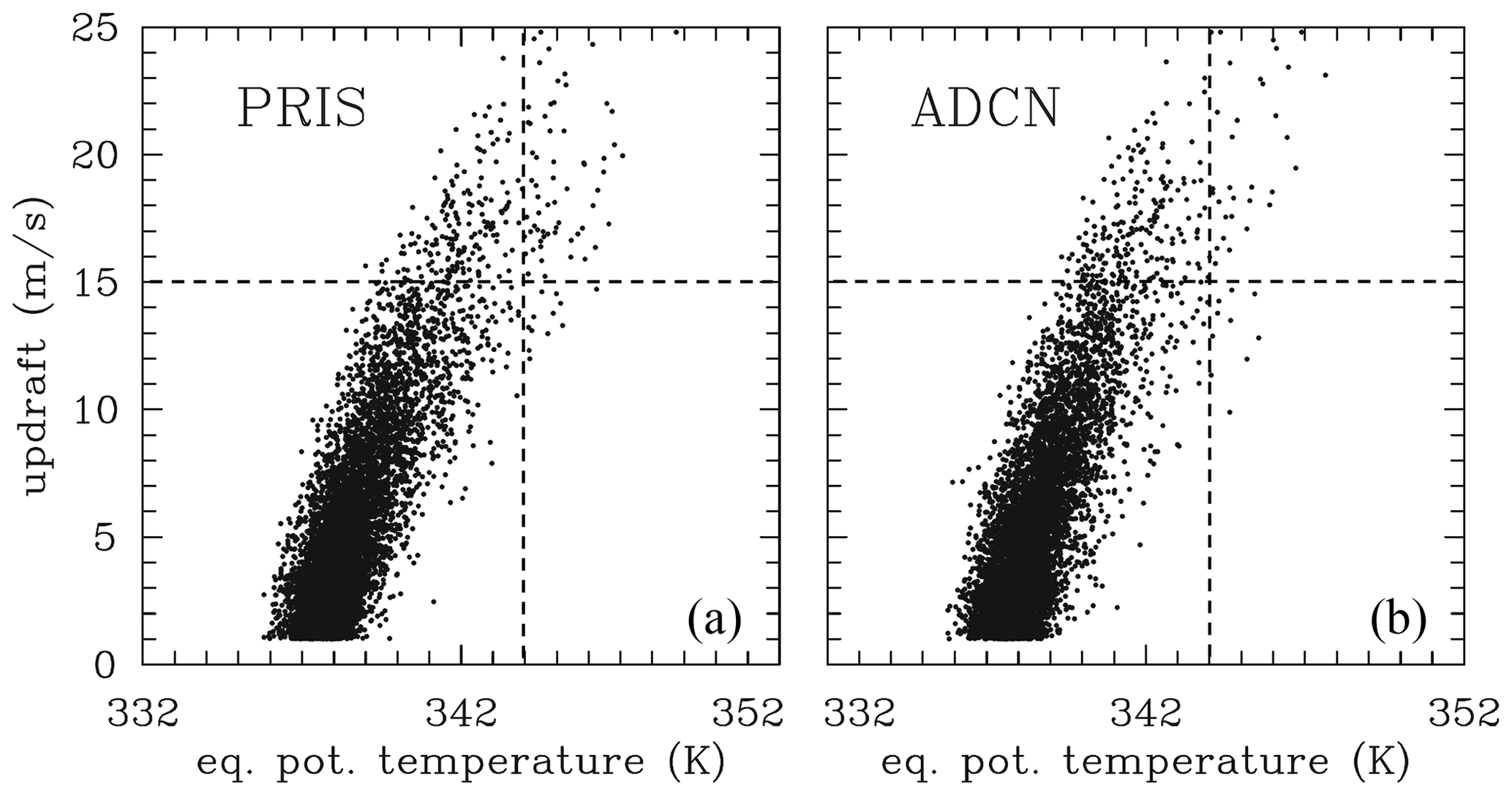
Figure 6 Like Fig. 5, but at 9 km for 2MOM (a) PRIS and (b) ADCN. Dashed horizontal and vertical lines show values of 15 m s⁻¹ and 344 K.

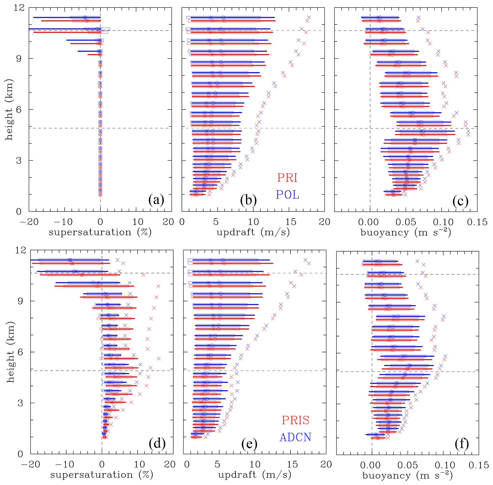
Figure 7 Statistics of (a, d) supersaturation, (b, e) vertical velocity, and (c, f) buoyancy in grid volumes with updraft larger than 1 m s⁻¹ and total condensate larger than 1 g kg⁻¹. (a–c) Data for all ensemble members for the 6th and 7th hours of the simulations from PRI (red color) and POL (blue color) IAB ensembles. (d–f) Data for all ensemble members for PRIS (red color) and ADCN (blue color) for 2MOM ensembles. The star/circle symbols are for median/mean values, horizontal lines show the 10th to 90th percentile range, and the boxes show the range between the mean and plus and minus 1 standard deviation. The × symbols to the right of color lines and boxes are means of the data from the range between the 90th percentile and the maximum. The data are only shown every second model level with color lines and symbols shifted above (for ADCN) and below (for PRIS) that level. Dashed horizontal lines show approximate height of the 0 and −40 ^∘C level. Dashed vertical lines in (a) and (c) show zero values.

Figure 6 shows similar results as Fig. 5 but at 9 km height and only for PRIS and ADCN ensembles. Compared to Fig. 5, updrafts are stronger than at 4 km (consistent with higher buoyancy and the increase in cCAPE with height; see Fig. 1), the equivalent potential temperature maxima are lower (i.e., more dilution), and there is less scatter. The difference between PRIS and ADCN seems to be absent (the latter is also true for IAB ensembles and no-wind 2MOM ensembles; not shown). The mean updraft for the 5 to 10 m s⁻¹ range is 7.06/7.08 m s⁻¹ for 2MOM's PRIS/ADCN and 7.13/7.11 m s⁻¹ for IAB's PRI/POL, that is, only slightly larger for the saturation-adjustment IAB simulations. The latter is not surprising as ice microphysics takes over at that height, as illustrated in Fig. 7, to be discussed shortly. For the 10 to 20 m s⁻¹ range, the mean values are 12.1 m s⁻¹ for both PRIS and ADCN from 2MOM ensembles and 13.1/12.9 m s⁻¹ for PRI/POL from IAB.

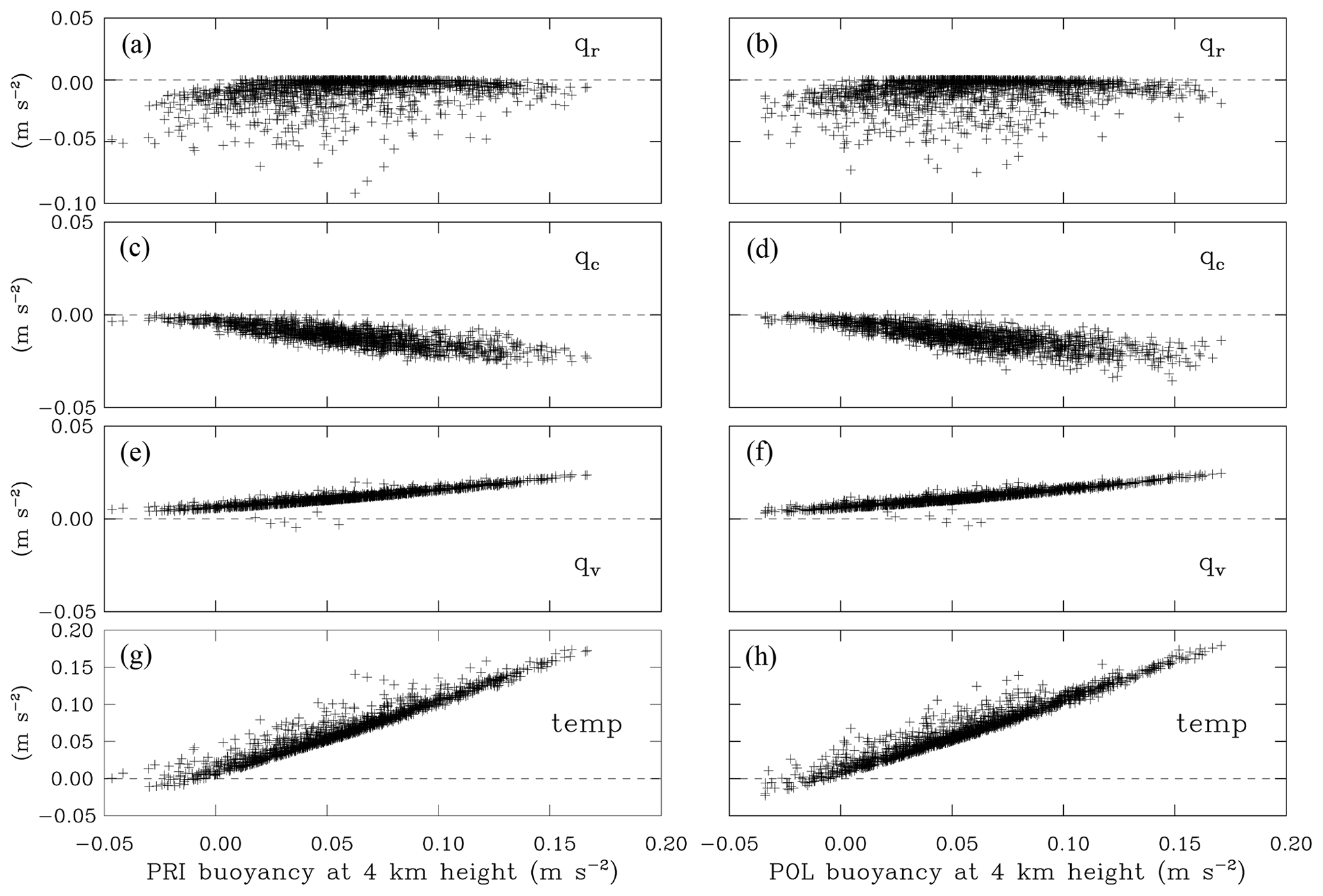
Figure 8 Scatterplots of buoyancy components at 4 km as a function of the total buoyancy in (a, c, e, g) PRI and (b, d, f, h) POL of all four ensemble members of IAB simulations at hours 6 and 7. The horizontal axes in both columns represent the total buoyancy. Panels (g) and (h) show the temperature buoyancy component. Panels (e) and (f) show the water vapor contribution. Panels (a)–(d) are the loading buoyancy components, separated into (c, d) cloud water and (a, b) rain components. Points with updraft larger than 1 m s⁻¹ and total condensate larger than 1 g kg⁻¹ are included. Only about 8 % of data points are shown.

4.2 Supersaturation, buoyancy, and updraft statistics

Figure 7 shows profiles of the supersaturation, updraft, and buoyancy statistics for rising (updraft larger than 1 m s⁻¹) cloudy (total condensate larger than 1 g kg⁻¹) volumes for ensemble members during hours 6 and 7 from IAB and 2MOM (PRIS and ADCN only for the latter). The overall impression is that the statistics look fairly similar between the two figures with the exception of the supersaturation. The supersaturation statistics for IAB show that the model's saturation adjustment works correctly in the lower and middle troposphere. Only above 9 km do ice processes allow supersaturation in ascending cloudy volumes to become subsaturated with respect to liquid water, resulting in a range of subsaturation values. The range of subsaturation above 9 km seems similar between IAB and 2MOM ensembles. For 2MOM, supersaturations can be significant (several percent), with the mean values (slightly lower for ADCN) ranging from 1 % to 5 % below the freezing level. The mean of the 90th percentile to the maximum range in Fig. 8 increases with height and reaches values close to $\mathrm{10}\mathit{\%}/\mathrm{15}\mathit{\%}$ in the middle troposphere for ADCN/PRIS ensembles.

Large supersaturation differences between IAB and 2MOM ensembles and differences between PRIS and ADCN lead to noticeable differences in the buoyancy statistics, in agreement with the discussion in Grabowski and Jarecka (2015) and Grabowski and Morrison (2017). In the lower and middle troposphere, buoyancies are significantly larger in IAB ensembles when compared to 2MOM and slightly larger in ADCN when compared to PRIS. The mean and the maximum buoyancies increase with height below the melting level in all ensembles (in agreement with the parcel analysis; Fig. 1), reach maximum values near the melting level, and then level off. Although the buoyancies do include all terms shown in Eq. (1), the maxima near the melting level are only slightly smaller than the values predicted by the adiabatic parcel, that is, around 0.15 and 0.13 m s⁻² for S = 0 % and S = 10 %, respectively, at 4 km in Table 2.

Despite the differences in the supersaturation and buoyancy, overall updraft statistics are similar. Maximum updraft vertical velocities increase with height in agreement with the parcel analysis (Fig. 1) and buoyancy statistics in the cloud model simulations. Below the freezing level, updrafts are stronger in IAB than in 2MOM, especially at the maximum end. At the freezing level, the mean updraft values of the 90th percentile to the maximum range are around 11 m s⁻¹ in IAB ensembles and around 7 and 8 m s⁻¹ in PRIS and ADCN, respectively. Above the 0 ^∘C level, the mean updraft values of the 90th percentile to the maximum range increase with height similarly between all ensembles, and they reach 15 to 20 m s⁻¹ in the upper troposphere. Results for the no-wind 2MOM ensembles (PRIS.NW and ADCN.NW) are similar to those shown in Fig. 7 and thus are not shown.

Although not directly relevant to the main thrust of this paper, it is worthwhile to mention that the convective mass flux is also insignificantly affected by small differences in the convective dynamics documented in Fig. 7. This is because cloud fraction profiles are only weakly affected by microphysical processes (at least before significant anvils develop in 2MOM simulations) as shown in G15 (Fig. 4 therein), Grabowski and Morrison (2016; Fig. 1 therein), and GM20 (Fig. 1 therein). Arguably, Fig. 2 herein documents that as well.

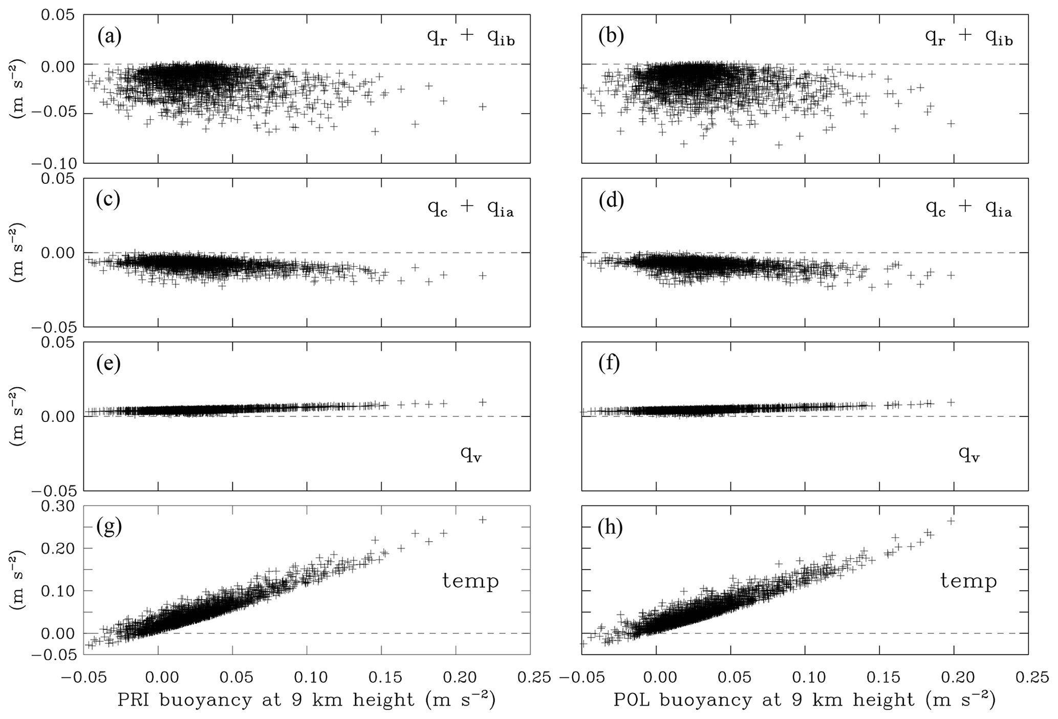
Figure 9 Like Fig. 8, but at 9 km. Panels (a, b) include rain combined with ice B mixing ratios; panels (c, d) include cloud water combined with ice A mixing ratio.

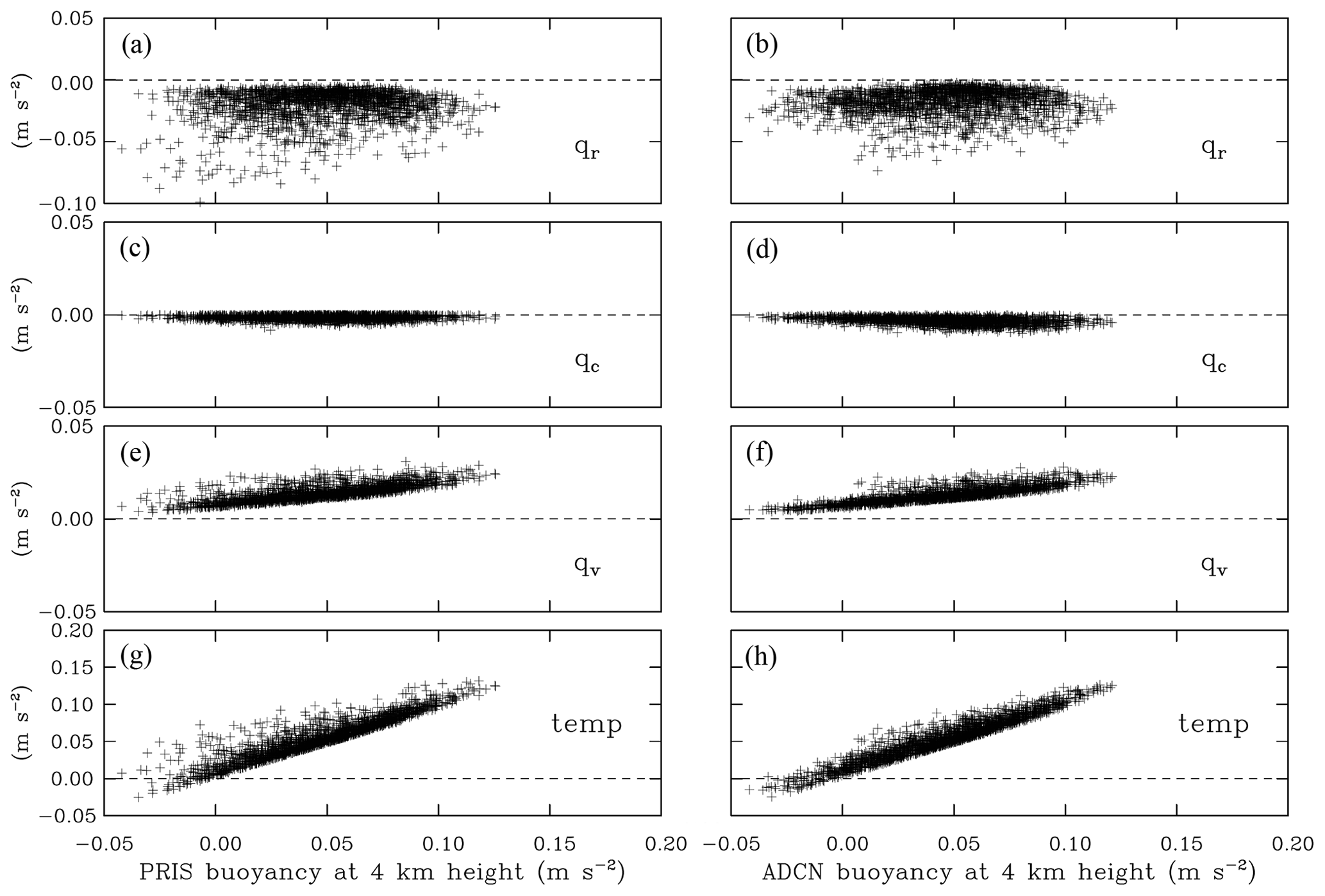
Figure 10 Like Fig. 8, but for all seven simulations of (a, c, e, g) PRIS and (b, d, f, h) ADCN from 2MOM ensemble. Only 5 % of data points are shown.

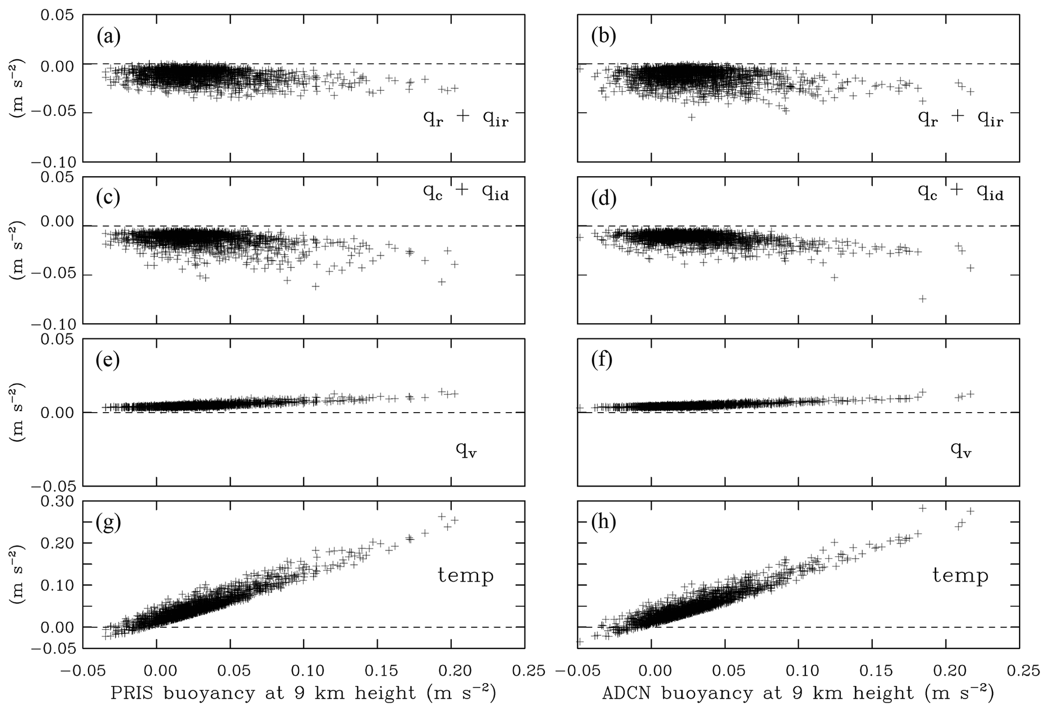
Figure 11 Like Fig. 10, but at 9 km. Panels (a, b) include rain mixing ratio combined with ice mixing ratio grown by diffusion of water vapor; panels (c, d) include cloud water combined with ice mixing ratio grown by riming.

4.3 Buoyancy analysis

To understand buoyancy differences better in 2MOM simulations and the lack thereof in IAB, Figs. 8 to 11 show contributions of buoyancy components as a function of the total buoyancy at 4 and 9 km for the IAB ensembles (Figs. 8 and 9) and 2MOM ensembles (Figs. 10 and 11) for grid volumes with updraft velocities larger than 1 m s⁻¹ and total condensate (cloud plus precipitation) larger than 1 g kg⁻¹. Buoyancy components represent the three terms in Eq. (1): the temperature, virtual, and loading components. In addition, the loading component is split into cloud and precipitation contributions (e.g., cloud water and rain at 4 km) as discussed below. Overall, the four figures show a coherent picture of the buoyancy contributions, with only small differences between the four ensembles. In agreement with the discussion above, IAB ensembles reach larger buoyancy values (note different buoyancy ranges on the horizontal axes in Figs. 8–11). In all four ensembles, the temperature term (i.e., the latent heating) provides the largest contribution. The temperature contribution increases linearly with the total buoyancy, with some scatter. The temperature contribution is aided by water vapor (i.e., the virtual temperature effect, especially at 4 km) and offset by the loading. For IAB at 4 km (Fig. 8), the loading includes only cloud water and rain, but at 9 km in Fig. 9 cloud liquid and ice A are merged together to represent “cloud condensate”, and rain and ice B are combined as “precipitation”. There are almost no differences between PRI and POL (i.e., left and right panels) in Figs. 8 and 9, consistent with saturation adjustment and just different flow realizations. The largest buoyancies are in volumes with relatively small contributions from the loading (especially at 9 km; Fig. 9), and the maximum buoyancies are not far from the pseudo-adiabatic parcel analysis values shown in Table 2, which excludes the loading.

For the 2MOM ensembles (Figs. 10 and 11), the maximum buoyancies are smaller than for IAB, but the patterns are similar. For the loading at 9 km (Fig. 11), the ice mass mixing ratio grown by diffusion of water vapor (q_id) is included in the “cloud condensate” contribution and the ice mass mixing ratio grown by riming (q_ir) in the “precipitation condensate”. Although there are small differences between PRIS and ADCN in total buoyancy as seen in Fig. 8, mainly below 5 km, these differences are not readily apparent in Figs. 10 and 11 when partitioned into the various contributions.

In the following analysis, we focus on the 2MOM simulations to better understand the buoyancy differences in PRIS and ADCN ensembles. We take advantage of the piggybacking technique that was used in G15, Grabowski and Morrison (2016, 2017), and in GM20.⁴ Piggybacking applies two sets of thermodynamic variables (the temperature, water vapor, and all aerosol, cloud, and precipitation variables) in a single cloud field simulation. The first set is coupled to the dynamics and drives the simulation; hence the driver. The second set, the piggybacker, is carried by the simulated flow and is modified by the same physical processes as the driver (e.g., surface fluxes, latent heating, precipitation fallout, etc.), but it does not affect the flow (see Grabowski, 2019, for the discussion and examples of application). Because every grid volume features two sets of cloud and thermodynamic variables (i.e., from the driver and from the piggybacker), these variables can be directly compared grid point by grid point instead of using conditional sampling. As a result, piggybacking allows one to separate the impact of a physical process (e.g., diffusional growth of cloud droplets or conversion from cloud water to rain) from the effects of different flow realizations.

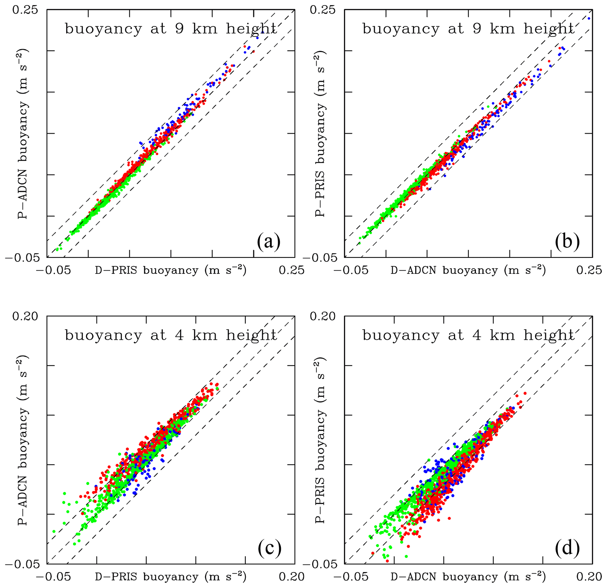
Figure 12 Driver versus piggybacker buoyancy at (a, b) 9 km and (c, d) 4 km height and hours 6 and 7 for all members of PRIS and ADCN ensembles. Driver buoyancy is shown on the horizontal axes (D-PRIS in a and c and D-ADCN in b and d). Piggybacker buoyancy is on the vertical axes. Symbol colors represent vertical velocity at the location from which driver and piggybacker buoyancies are taken. At 4 km, green, red, and blue represent updrafts between 1 and 5, 5 to 10, and above 10 m s⁻¹, respectively, with only 2 % of all points shown for green, 10 % for red, and all for blue. At 9 km, green, red, and blue colors represent updrafts between 1 and 10, 10 to 20, and above 20 m s⁻¹, with 4 % of all points shown for green, 20 % for red, and all for blue. Middle dashed lines show equal buoyancies, and the lines above and below show buoyancies offset by 0.02 m s⁻². Only points with vertical velocity larger than 1 m s⁻¹ and total condensate mixing ratio larger than 1 g kg⁻¹ are included in the plot.

Figure 12 shows scatterplots of the driver versus piggybacker buoyancies for the PRIS and ADCN ensembles at 4 and 9 km during the 6th and 7th hours of the simulations with colors indicating the updraft velocity. The same dataset (although only for hour 6 and without colors) was used to show similar scatterplots at 3 and 7 km in Fig. 5 of GM20. At 4 km, ADCN buoyancies are larger than for PRIS (with a few exceptions) regardless if ADCN drives (Fig. 12d) or piggybacks (Fig. 12c) the simulation. The larger buoyancies correspond to larger vertical velocities (i.e., red and blue symbols), but the scatter is significant perhaps because the local updraft magnitude represents the time-integrated buoyancy, not the current location value (as well as integrated impacts of perturbation pressure forcing). The differences at 4 km are relatively small, typically below 0.02 m s⁻², especially when comparing the magnitude of extreme buoyancies shown in Fig. 10. Only a small fraction of points shows larger differences, especially in the 0 to 0.05 m s⁻² range. Red points (updrafts in 5 to 10 m s⁻¹ range) typically show larger buoyancies for the ADCN ensemble (consistent with the supersaturation differences), whereas blue points (updrafts above 10 m s⁻¹) are scattered both above and below the 1:1 line, showing contrasting impacts of the temperature and loading contributions (increasing/reducing buoyancy for the former/latter in the ADCN ensemble as shown in Fig. 14 below). A combination of the temperature and loading terms arguably explains the small differences in the largest updraft velocities between PRIS and ADCN as shown in Figs. 5 and 7. Driver–piggybacker differences at 9 km are smaller, with ADCN buoyancies typically slightly larger regardless if ADCN drives or piggybacks the flow. The scatter is smaller than at 4 km, perhaps in agreement with smaller scatter of the equivalent potential temperature at 9 km (see Fig. 4a). In contrast to the 4 km plots, a clear trend of larger driver–piggybacker differences for larger buoyancies is evident. In addition, the strongest updrafts tend to correspond to the largest buoyancies, also in some contrast to the 4 km statistics.

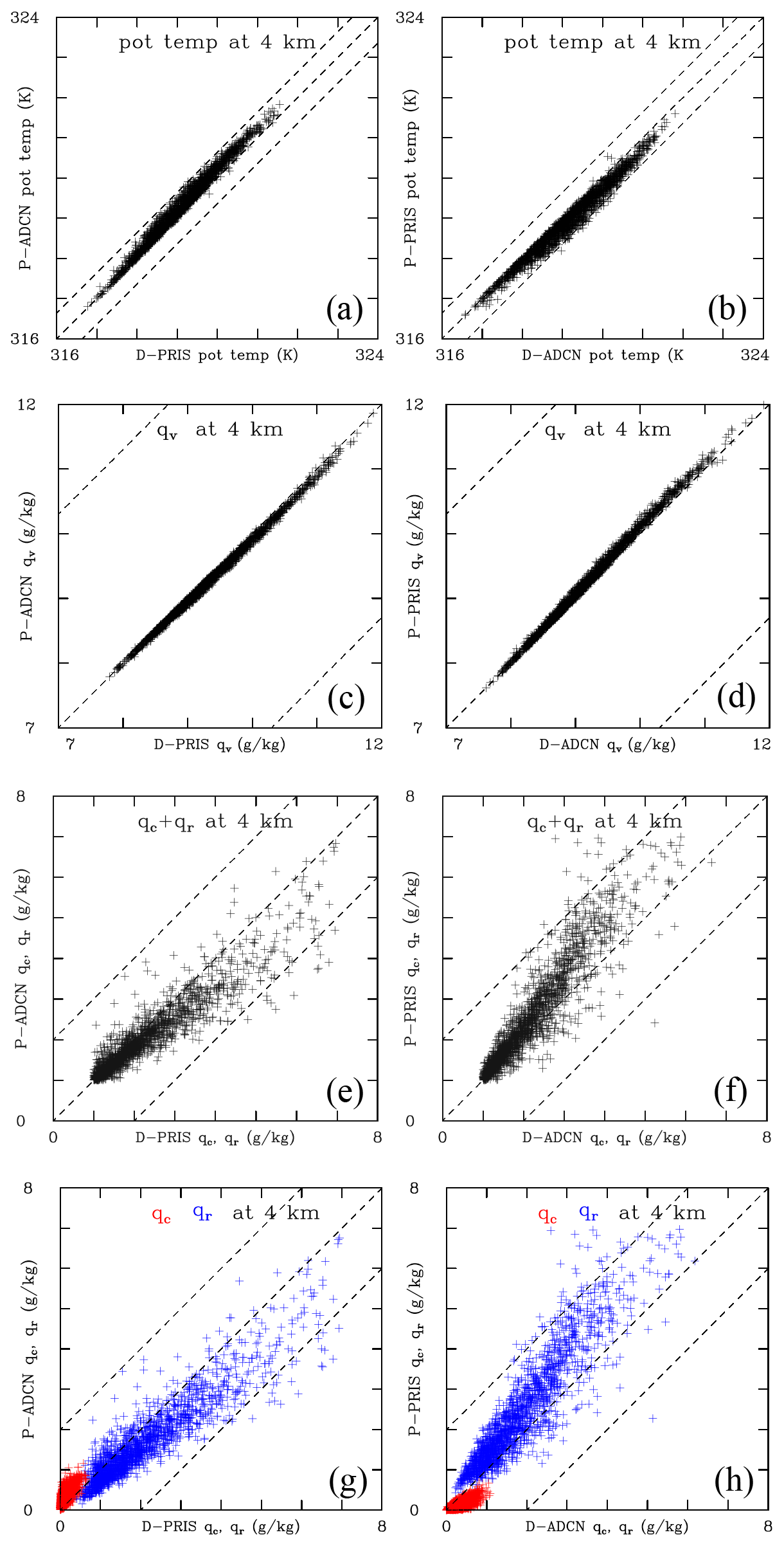
Figure 13 Driver versus piggybacker for components of the buoyancy at 4 km shown in the lower panels of Fig. 12. (a, b) Temperature, (c, d) water vapor, (e, f) total loading, and (g, h) loading split into cloud water (red) and rain (blue). Dashed lines below and above the 1:1 dashed line in all panels correspond to the buoyancy impact as shown by dashed lines in Fig. 12. Only 5 % of data points with the vertical velocity larger than 1 m s⁻¹ and the total condensate larger than 1 g kg⁻¹ are used.

Figure 14 Like in Fig. 13, but for the upper panels of Fig. 13, that is, at 9 km height. Dashed lines for q_v (middle panels) are outside the range of q_v values shown in the figure. The total loading component in (e, f) is split in (g, h) between cloud water (red), ice mixing ratio grown by diffusion of water vapor (black), and ice mixing ratio grown by riming (blue).

Figures 13 and 14 show scatterplots in a similar format as Fig. 12 but contrasting buoyancy components between PRIS and ADCN ensembles at 4 km (Fig. 13) and 9 km (Fig. 14). The figures show buoyancy components for the temperature (Fig. 13a, b and Fig. 14a, b), water vapor (Fig. 13c, d and Fig. 14c, d), and condensate (Fig. 13e–h and Fig. 14e–h), the latter showing total condensate and cloud and rain water separately in Fig. 13 with ice components added in Fig. 14. Upper and lower dashed lines in the panels correspond to approximately the same impact of the perturbations on the buoyancy as dashed lines above and below the 1:1 line in Fig. 12 (i.e., around 0.02 m s⁻²). At 4 km (Fig. 13), the temperature and condensed water (cloud water and rain) differences are the largest contributors to the PRIS–ADCN buoyancy differences. The water vapor PRIS–ADCN difference adds little; even a 10 % difference in supersaturation and hence water vapor mixing ratio has little impact on buoyancy because the virtual temperature effect on buoyancy is already relatively small (see Fig. 10). The potential temperature is typically larger in ADCN than in PRIS regardless of whether it drives or piggybacks the simulation. One can argue (e.g., Fan et al., 2018) that this is consistent with smaller supersaturations and larger condensational growth in ADCN. However, since the driver and piggybacker experience the same updraft, the temperature difference has to come from the supersaturation being different from the quasi-equilibrium supersaturation. This is because, as mentioned in the “Introduction” and discussed in detail in Sect. 2b of GM20, the condensation rate (and thus the latent heating) for a given updraft is the same as long as the supersaturation is equal to the quasi-equilibrium supersaturation. In other words, for condensational growth, the driver and piggybacker temperatures would be the same if the supersaturation was equal to the quasi-equilibrium supersaturation. Another possibility is that the difference comes from entrainment, but this is unlikely as illustrated in Fig. 4 and its discussion.

Figure 13g and h show that cloud and rain water also contribute significantly to the buoyancy differences, aiding the temperature differences seen in Fig. 13a and b. Note that the analysis includes only points with the total condensate larger that 1 g kg⁻¹, and this explains why there are no points with total condensate smaller than that threshold in Fig. 13e and f. In Fig. 13g and h, the red symbols for cloud water in the lower Fig. 13g are above the 1:1 line which implies that ADCN has more cloud water, in agreement with the suppressed conversion from cloud water to rain in polluted conditions. (Note that these points have to come from volumes with rain because, to be included in the plot, the total condensate has to be larger than 1 g kg⁻¹.) As a result, the cloud water opposes the temperature ADCN–PRIS difference, but this is counterbalanced by the rain contribution that helps the temperature impact. Points for the D-PRIS versus P-ADCN rainwater in Fig. 13g (blue symbols) are below the 1:1 line. This implies that there is more rain water in the D-PRIS, again consistent with suppressed conversion of cloud water to rain in ADCN. At the same time, rain falls from above and also contributes negatively to the buoyancy at 4 km in D-PRIS. There is a significant scatter in the rain points, and there are some points at which rain is higher in ADCN, no doubt from the impact of rain sedimentation from higher levels in some grid volumes. The right panels (Fig. 13b, d, f, h) are close to mirror images of those in the left column (Fig. 13a, c, e, g). In summary, both the temperature difference (warmer in ADCN) and the loading difference (on average smaller in ADCN) contribute to the larger buoyancy in ADCN below the freezing level. However, the overall difference is small, as shown in Fig. 11. An important point is that the temperature and loading differences between PRIS and ADCN results can only be seen in the comparison applying piggybacking because they are not seen in Fig. 10 buoyancy analysis.

Figure 14 shows analogous results at 9 km. For the temperature, the outcome is similar to that at 4 km (Fig. 13), with ADCN being slightly warmer compared to PRIS, especially at the highest temperature end. Contributions from water vapor are even smaller than in Fig. 13, as expected, and this is why Fig. 14c and d do not show dashed lines (these are outside the range shown on the axes). For the cloud and precipitation condensate, the total impact (Fig. 14e and f) is small with some scatter around the 1:1 line. Figure 14g and h show the contributions from the cloud water and the two ice mixing ratios. The rain water is close to zero, and thus it is not shown. The cloud water range is similar to that at 4 km (up to ∼ 1 g kg⁻¹), and it contributes negatively to the ADCN–PRIS difference. The ice mixing ratio grown by diffusion of water vapor (q_id, black symbols) shows small ADCN–PRIS differences except for large mixing ratios which are larger in ADCN than PRIS ensembles in both the left and right panels. One possibility is that the higher ice crystal concentrations resulting from higher droplet concentrations at lower levels in the ADCN ensemble leads to a more efficient growth by the diffusion of water vapor, similar to the condensational growth of cloud droplets. The blue symbols for the ice mixing ratio grown by riming (q_ir) show a similar impact as that for rain at 4 km (i.e., below/above the 1:1 line in the left/right panels). This may come from frozen rain drops carried from lower levels (more abundant in the PRIS case), together with more efficient growth by riming for larger cloud droplets in the PRIS case. Comparing Fig. 14e, f and Fig. 14g, h clearly shows that there is a significant compensation between the mixing ratios of ice grown by vapor deposition and riming that together lead to a relatively small impact on total condensate differences between PRIS and ADCN.

In summary, the temperature and loading differences in the 2MOM simulations are fairly small and result in limited differences in the buoyancy and vertical velocity in PRIS and ADCN ensembles. The buoyancy and vertical velocities in 2MOM ensembles are smaller than in IAB because the saturation adjustment in IAB ensembles is replaced by the supersaturation prediction in 2MOM.

5 Conclusions

This paper investigates factors affecting cloud buoyancy using theoretical analysis and results from numerical simulations of scattered deep convection. The motivation comes from previous discussions of the so-called convection invigoration in polluted environments, that is, the increase in updraft speed resulting from the increase in the CCN concentrations. A recent exchange between Fan and Khain (2021) and Grabowski and Morrison (2021), and references in those papers, provides the context for the invigoration conundrum. The original claim (e.g., Andreae et al., 2004; Rosenfeld et al., 2008) hypothesized that suppression of rain formation in the lower troposphere in high-CCN environments, transport of the cloud water across the melting level, and freezing it aloft results in the invigoration of the upper-tropospheric updrafts. However, as discussed in Grabowski and Morrison (2020, Sect. 2a) and mentioned in the “Introduction”, the latent heat of freezing merely compensates for the loss of buoyancy due to carrying the extra liquid into the upper troposphere. Hence, the so-called “cold-phase invigoration” is difficult to justify on theoretical grounds. Fan et al. (2018) argue that the presence of lower supersaturations in polluted convective updrafts below the freezing level provides a different kind of invigoration that indeed has been seen in previous simulations (Grabowski and Jarecka, 2015; Grabowski and Morrison, 2017, 2020; see also Cotton and Walko, 2021). This has been referred to as “warm-phase invigoration” because the argument involves differences in the condensational growth of cloud droplets below the freezing level. However, physical mechanisms behind the warm-phase invigoration are unclear, especially when considered together with other processes affecting cloud buoyancy, such as the condensate loading, precipitation fallout, and entrainment.

We analyze a 2 h period of deep convection from 12 h long simulations of daytime convection development over land. The mean sounding from this period of the simulations serves as input to the theoretical analysis applying a rising parcel framework (see Fig. 3 and Table 2). For the pseudo-adiabatic parcel, that is, excluding parcel condensate loading, we contrast results obtained with different levels of the supersaturation maintained within the parcel, from 0 % (i.e., the traditional water-saturated parcel analysis) to 10 % supersaturation (with respect to water saturation) across the entire depth the parcel rises. In agreement with the previous theoretical analysis in Grabowski and Jarecka (2015), maintaining finite supersaturations results in a reduction in pseudo-adiabatic parcel buoyancy in the lower and middle troposphere, a several-percent reduction in the total CAPE, and a fairly large reduction in the cumulative CAPE in the lower troposphere (e.g., from about 300 to about 200 J kg⁻¹ at 4 km for 10 % supersaturation). Including loading in the parcel buoyancy, relative to the pseudo-adiabatic parcel with no loading, has a similar impact in the lower troposphere as going from 0 % to 10 % supersaturation (e.g., similar cCAPE reduction at 4 km), but it is much more significant in the upper troposphere. This occurs because the supersaturation impact on parcel buoyancy decreases with height, but the condensate carried by the adiabatic parcel increases, approaching near-surface water vapor mixing ratios, over 15 g kg⁻¹, in the upper troposphere. For an adiabatic parcel with all the condensate included in the parcel buoyancy, the total CAPE is about 40 % of the pseudo-adiabatic CAPE. In agreement with numerous past observational and modeling studies of deep convection, the impact of entrainment on parcel buoyancy and cCAPE is large, with a relatively small bulk fractional entrainment rate of 0.05 km⁻¹ reducing total CAPE by about 40 %. Larger entrainment rates lower the equilibrium level of the parcel from the upper to the middle troposphere and substantially reduce cCAPE. The magnitude of cCAPE changes from finite supersaturation is not affected by condensate loading or entrainment. However, because loading and entrainment reduce cCAPE, the relative impacts of finite supersaturation increase.

The impact of the supersaturation, entrainment, and loading is further quantified in the analysis of the numerical simulations. The simulations use either a simple single-moment bulk scheme with saturation adjustment, the IAB set of simulations, or a more comprehensive double-moment bulk scheme with supersaturation prediction, the 2MOM simulation set. Overall, IAB and 2MOM ensembles feature similar convective cloud field evolutions (at least before only upper-tropospheric anvils are left in the simulations) despite significant differences in the microphysics parameterizations. The difference between pristine and polluted CCN conditions is simulated by assumed contrasting cloud droplet concentrations in the IAB simulations (Grabowski, 2015; G15) or by specifying contrasting CCN spectra in the 2MOM simulations (Grabowski and Morrison, 2020; GM20). For analyzing entrainment, we use a simplified formulation of equivalent potential temperature Θ_e equal to the moist static energy divided by c_p, a conserved variable for ice-free conditions and only slightly modified when ice is present (the latter is because the latent heat of freezing is only a small fraction of the latent heat of condensation). Profiles of cloud updraft Θ_e statistics (Fig. 4) document a significant dilution by the entrained environmental air, with small differences between pristine and polluted conditions. Profiles of the median Θ_e correspond to a bulk fractional entrainment rate of about 0.20 km⁻¹, whereas profiles of the 90th percentile can be explained by a bulk fractional entrainment rate around 0.13 km⁻¹. These values are consistent with the idealized parcel simulations and vary insignificantly between 2MOM pristine and polluted simulations. The strongest updrafts, slightly stronger in the saturation-adjustment IAB simulations (see Fig. 5), occur in the least diluted cloudy volumes, with small differences between pristine and polluted 2MOM simulations. The impact of entrainment in the theoretical analysis and in model simulations based on median updraft properties versus those of strongest updraft cores is reminiscent of the old cloud physics problem of representing convective cloud properties using one-dimensional models (e.g., Warner, 1970): a large entrainment is needed to represent overall cloud dilution, while at the same time only small entrainment rates ensure that the cloud depth (controlled by relatively less dilute parcels) is correctly represented.

For the impact of finite supersaturation, we compare profiles of supersaturation, buoyancy, and updraft statistics between IAB simulations featuring saturation adjustment with 2MOM simulations that predict the in-cloud supersaturation. Finite supersaturations indeed provide a noticeable reduction in the updraft buoyancies and vertical velocities in the lower and middle troposphere, with small differences between pristine and polluted conditions below and around the freezing level (Fig. 7). Analysis of in-cloud updraft buoyancies (Figs. 8–11) documents that the temperature term is the most significant buoyancy component (in agreement with the elementary arguments in the “Introduction”), and it is opposed by the cloud and precipitation loading, especially below the freezing level in both IAB and 2MOM simulations (Figs. 8 and 10). Aloft, the largest buoyancies typically correspond to small loading; see Figs. 9 and 11. Overall, buoyancy contributions in IAB and 2MOM simulations are similar, except for somewhat larger buoyancy maxima below the freezing level, as mentioned above.

Because these simulations apply the piggybacking technique (i.e., each simulation carries two sets of thermodynamic variables, one driving and one piggybacking the simulated flow), the impact of assumed CCN conditions on the buoyancy can be directly (i.e., point-by-point) compared between pristine and polluted conditions. The difference in the lower troposphere comes from concurring differences in the temperature (due to latent heating) and loading. Because the driver and piggybacker experience the same cloud flow, the temperature difference must be explained by either the supersaturation being different from its quasi-equilibrium value or entrainment and mixing of temperature being different. The quasi-equilibrium supersaturation represents a balance between the supersaturation sink due to droplet diffusional growth and supersaturation source due to rising air motion. The key point is that the condensation rate is independent of the droplet concentration and size, and it depends only on the vertical velocity, as long as the supersaturation is equal to its quasi-equilibrium value; see Sect. 2b in GM20. Because our entrainment analysis shows similar behavior for pristine and polluted conditions (see Sect. 4.1), the temperature difference can only be explained by the updraft supersaturations being different from their quasi-equilibrium values. At 4 km height (Fig. 13), slightly higher temperatures in the polluted case when compared to the pristine case are aided by the loading, larger in the pristine case and in agreement with suppressed rain formation in the polluted case. Temperature and loading differences at 9 km height are smaller (Fig. 14), with an intriguing compensation between loading contributions from the ice mass grown by diffusion and that grown by riming.

Overall, the analysis presented in this paper is consistent with the theoretical study of Igel and van den Heever (2021) and suggests that the impact of CCN characteristics on convective dynamics is rather subtle and requires detailed analysis (e.g., through piggybacking) to understand the physical processes involved. Perhaps the most significant difference from the modeling point of view is a contrast between the strongest updrafts when applying a microphysical scheme with saturation adjustment and one with supersaturation prediction, stronger in the former case (Grabowski and Morrison, 2017; Zhang et al., 2021). In 2MOM simulations applying a scheme that predicts the in-cloud supersaturation, the differences between pristine and polluted conditions are rather small. How the latter depends on the particular microphysical scheme and whether it changes when a more sophisticated microphysics scheme is used (e.g., bin microphysics as in Zhang et al., 2021, or Lagrangian microphysics as in Shima et al., 2020) need to be investigated in the future.