the Creative Commons Attribution 4.0 License.
the Creative Commons Attribution 4.0 License.
 | 01 Sep 2021
Development of a new emission reallocation method for industrial sources in China
Chi Chiu Cheung
Xuguo Zhang
Joshua S. Fu
Jimmy Chi Hung Fung
An accurate emission inventory is a crucial part of air pollution management and is essential for air quality modelling. One source in an emission inventory, an industrial source, has been known with high uncertainty in both location and magnitude in China. In this study, a new reallocation method based on blue-roof industrial buildings was developed to replace the conventional method of using population density for the Chinese emission development. The new method utilized the zoom level 14 satellite imagery (i.e. Google®) and processed it based on hue, saturation, and value (HSV) colour classification to derive new spatial surrogates for province-level reallocation, providing more realistic spatial patterns of industrial PM2.5 and NO2 emissions in China. The WRF-CMAQ-based PATH-2016 model system was then applied with the new processed industrial emission input in the MIX inventory to simulate air quality in the Greater Bay Area (GBA) area (formerly called Pearl River Delta, PRD). In the study, significant root mean square error (RMSE) improvement was observed in both summer and winter scenarios in 2015 when compared with the population-based approach. The average RMSE reductions (i.e. 75 stations) of PM2.5 and NO2 were found to be 11 µg m−3 and 3 ppb, respectively. Although the new method for allocating industrial sources did not perform as well as the point- and area-based industrial emissions obtained from the local bottom-up dataset, it still showed a large improvement over the existing population-based method. In conclusion, this research demonstrates that the blue-roof industrial allocation method can effectively identify scattered industrial sources in China and is capable of downscaling the industrial emissions from regional to local levels (i.e. 27 to 3 km resolution), overcoming the technical hurdle of ∼ 10 km resolution from the top-down or bottom-up emission approach under the unified framework of emission calculation.
- Article
(10127 KB) - Full-text XML
-
Supplement
(3700 KB) - BibTeX
- EndNote


The emission inventory is essential for air quality management and climate studies. Various applications, including setting up regional emission reduction targets and performing numerical air quality forecasts, rely upon an accurate inventory for sound assessment and judgement (Krzyzanowski, 2009; Zhao et al., 2015). As the purpose and type of emission inventories (e.g. point, mobile, and area) vary largely, data requirements and collection methods can be quite different (Kurokawa et al., 2013). In point source inventory, collecting large point sources (i.e. power plant) is generally straightforward, while obtaining data from scattered industrial sources often poses challenges and requires tremendous effort to collect and process. In developed countries like the USA, industrial sources are usually large, but they do not always contribute to a dominant portion in the emission inventory (e.g. 10 %–15 % in PM10 and 25 %–60 % in NMVOC), and the data collection process is commonly incorporated into routine permitting exercise, making it easy to be included in their national inventory (ECCC, 2017; Janssens-Maenhout et al., 2015; Lam et al., 2004). Unfortunately, this is not the case for developing countries like China where industrial sources are considered as a major emitter; Li et al. (2017) reported that industrial sources from non-power generation (NPG) are the largest contributors of PM10 and NMVOC in the MIX inventory. With the infinite numbers of small factories scattered across the continent and frequent changes of location caused by urban redevelopment, these industrial sources are often treated as an area or non-point source regardless of whether it is a point source (e.g. stack) or not. Hence, there are large spatial uncertainties in the inventory.
In recent years, various Asian emission inventories (e.g. REAS, MIX, and MICS-ASIA) have been developed for the purpose of air pollution modelling and have been widely used for studying transboundary air pollution among Asian countries (Chen et al., 2019; Tan et al., 2018). The top-down or semi-bottom-up approach based on the unified framework of source categories, calculating method, chemical speciation scheme, and spatial and temporal allocations was commonly used in the emission inventory development, where emissions were handled separately for different source categories (e.g. power, industry, transport, residential/domestic, and agriculture) with limited spatial resolutions ranged from 10 to 27 km (Kurokawa et al., 2013; Li et al., 2017; Ohara et al., 2007; Streets et al., 2003). In some cases, higher-resolution emission inputs were achieved via GIS spatial interpolation for subregional (i.e. 10–15 km resolution) application. Information such as stack location, road network, and population density was applied as surrogate data for spatial reallocation (Du, 2008). For the case when ultra-high resolution (i.e. 1–3 km resolution) was needed, it was often supplemented with the bottom-up approach using the detailed activity data (i.e. exact emission locations and its relevant emission amounts) in the emission inventory development (HKEPD, 2011). For the category of small to medium industrial sources where location information was frequently missing in the top-down or semi-bottom-up emission approach, the population density was used as the surrogate, given the fact that population density was considered a good proxy for accessing employment, goods, and services (Giuliano and Small, 1993). Historically, this approach seemed to be quite robust to capture the factory location due to (1) the Danwei/socialist work units which enforced jobs and residences to be close to each other to reduce travel distance (Yang, 2006), and (2) factory jobs typically included accommodation (i.e. dormitory) for attracting foreign workers. With limited transport infrastructure, dormitories were usually within a few kilometres away from the factories. However, in recent years, the land-use and housing reforms in China have led to a spatial separation of jobs and residences, and the strong factory-residence pattern has slowly diminished in Chinese cities as efficient public transportation has emerged. With the adaptation of industrial parks in the urban renewal process, the separation of industrial-related employment (on the outskirts of the city) from residential space (city centre) was further expedited (Zhao et al., 2017). As a result, there is a need to reconsider how industrial emissions are handled in the top-down or semi-bottom-up emission approach, searching for a suitable surrogate for the emission reallocation.
In this study, the concept of a blue-roof industrial surrogate was introduced for the first time for Chinese industrial emission allocation. The approach assumed the majority of industrial buildings (both factories and warehouses) in China were single-story non-concrete buildings with their rooftop made out of galvanized metal coated with blue epoxy. In this development, satellite imagery with zoom level 14 (i.e. Google®) was adopted and processed with HSV-based colour classification for generating the province-level spatial surrogate. The Community Multi-Scale Air Quality (CMAQ) PATH-2016 platform with 3km MIX inventory was then applied to evaluate the impacts of air quality predictions between population and blue-roof-based methods, and the simulated results of PM2.5, NO2, and O3 were then compared to local observation data and CMAQ results from the point- and area-based bottom-up approach (hereafter referred to as “btmUp case”) from Zhang et al. (2020) to assess its model performance (HKEPD, 2011; Li et al., 2017).
A new allocation method called “blue-roof” industrial allocation was introduced in the top-down or semi-bottom-up emission approach for better allocating the scattered NPG industrial emissions in China. In this study, the CMAQ model and the regional Asian emission inventory MIX were applied to evaluate the effectiveness of the new allocation method on the performance of air quality prediction. The target simulation year is 2015, and the details of each component are described below.
2.1 Study area, simulation domain, and observation network
The Guangdong–Hong Kong–Macao Greater Bay Area (GBA), also known as the Pearl River Delta (PRD), was adopted as the study area for the industrial allocation test. The characteristic of diverse industrial clusters (e.g. garment, electronics, and plastic factories) scattered across the area creates an ideal testbed for spatial examination. The GBA area consists of two special administrative regions (Hong Kong and Macao) and nine Chinese municipalities, including Guangzhou, Shenzhen, Zhuhai, Foshan, Huizhou, Dongguan, Zhongshan, Jiangmen, and Zhaoqing in Guangdong Province with a total area coverage of over 56 000 km2. It is classified as one of the world-class manufacturing hubs in China. In this study, the CMAQ-based PATH-2016 was adopted to evaluate the influence of air quality prediction from the new allocation method. The PATH-2016 modelling platform consists of four nested domains, including East Asia and Southeast Asia (D1), southeastern China (D2), GBA/PRD (D3), and Hong Kong (D4) with resolutions of 27, 9, 3, and 1 km, respectively. For this study, only D1–D3 was applied as it already covered the entire GBA with a reasonable spatial resolution (e.g. 3 km) for regional air quality simulation, as shown in Fig. 1. Details of PATH-2016 and its model setting are discussed in a later section. For evaluating the performance of CMAQ air quality prediction, the China National Environmental Monitoring Centre (CNEMC) and the Guangdong-Hong Kong-Macao Pearl River Delta Regional Air Quality Monitoring Network (HKEPD, 2016) with over 75 surface observation stations were adopted (available at http://www.cnemc.cn/, last access: 10 September 2020). These stations measure various air pollutants, including PM2.5, PM10, SO2, NO2, and O3.
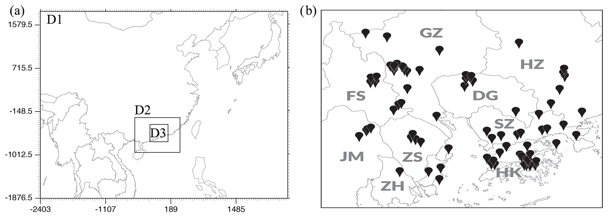
Figure 1(a) CMAQ simulation domains and (b) D3 domain with observations.
2.2 PATH-2016 and MIX inventory
The PATH-2016 is a WRF-CMAQ (Community Multi-Scale Air Quality model) Air Quality system used by the HKSAR government for air-quality-related policy. It has been validated in several studies (HKEPD, 2011, 2019; Zhang, 2020). In this study, CMAQ version 5.0.2 with an AERO5 aerosol module and CB05CL carbon bond chemical mechanism driven by WRF version 3.7.1 was adopted for air quality simulation. The model set-up for CMAQ simulation is summarized in Table 1, and WRF meteorological validation can be found in Zhang (2020) and HKEPD (2019). The initial and boundary conditions for the outermost domain, D1, were generated from the global model GEOS-Chem outputs for Asian pollution background (Lam and Fu, 2010). In terms of the model emissions, the majority of the anthropogenic emissions were adopted from the Asian emission inventory, MIX. The MIX is a regional emission inventory developed to support the Model Inter-Comparison Study for Asia (MICS-Asia) and the Task Force on Hemispheric Transport of Air Pollution (TF HTAP) (Li et al., 2017). It consists of five anthropogenic emission source categories, including point, industry, transport, residential, and agriculture (NH3 only) with a resolution of 0.25∘ (∼ 27 km), and its emission base year is 2010. In this study, the MIX inventory was first scaled to the target simulation year of 2015 based on available sector-based control technologies (Li et al., 2019; Zhang, 2020; Zheng et al., 2018). The derived emission totals from each sector, except for the industrial emissions, were then temporally and spatially interpreted into 27 km (D1), 9 km (D2), and 3 km (D3) resolutions using the top-down emission method described in Du (2008). Detailed methodology and validation of the base year 2015 emission inventory were extensively discussed and can be found in our previous publications (Zhang et al., 2021, 2020). As Hong Kong emissions were not well presented in the MIX inventory due to the limitation of spatial resolution, the bottom-up emissions from the PATH-2016 platform were adopted for Hong Kong emissions. For the remaining sectors that were not available from the MIX inventory, it was adopted from the PATH-2016 study (Zhang, 2020). These include MEGAN biogenic, GFED biomass burning, marine, and sea-salt emissions (Athanasopoulou et al., 2008; Giglio et al., 2013; HKEPD, 2019; Ng et al., 2012).

2.3 Case study for non-point source industrial allocation
The purpose of CMAQ simulation is to evaluate the performance of the new industrial allocation method on air quality prediction in China. Two CMAQ scenarios tailored for the industrial allocation methods were proposed and tested with the MIX inventory. These scenarios are (1) a population-based method and (2) a blue-roof-based method. Details of each method are described in the later section. For each scenario, two months of CMAQ air quality simulation were performed. The selection of winter (January) and summer (August) months from 2015 was to allow better reflection of air quality impacts from the change of Asian monsoon in southern China. The choice of using 2015 as the based year was to permit more local observation data to be available in the GBA area from the Chinese national observation network (operated after late 2013), moreover, to better fit with the modelling effort in 2016 Air Quality Objectives (AQOs) review that has also applied PATH-2016 model (Zhang, 2020).
2.3.1 Base case – population-based method
The population-based method (hereafter referred to as “base case”) is commonly applied in the top-down emission inventory to allocate residential (area) or NPG industrial sector, in the regional emission inventory (Du, 2008; Li et al., 2017; Ohara et al., 2007). It utilizes population or population density as a spatial proxy to distribute the sectorial emissions into the simulation grids. It assumes a strong association is present between population and industrial emissions. In this study, the Oak Ridge National Laboratory (ORNL) LandScan global population data with the resolution of ∼ 1 km () gridded spatial resolution was applied to allocate industrial emissions. To allow the separation of the urban population from the rural population in LandScan grids, a threshold value of 1500 people per square kilometre was adopted, in which any grid values that were greater than this number were considered as urban grids (Liu et al., 2003). The basic equation for estimating the gridded emissions (Em,n) using urban population is shown in Eq. (1). Em is the total emission in a province (m), and is the ratio of urban population from a grid (n) to the province total. This value is commonly referred to as the spatial allocation factor, and it is a dimensionless value ranging between 0 and 1. The collection of spatial allocation factors in the gridded matrix is called a spatial surrogate. In this study, all the calculations and the spatial interpretation were performed in ArcGIS to yield CMAQ-ready emissions.
where Em,n is the emission in the nth grid for the mth province, Em is the total emission in the mth province, U_popn is the urban population count in the nth grid, and U_popm is the total population in the mth province.
2.3.2 Blue-roof case: blue-roof-based method
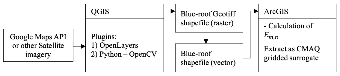
The “blue-roof-based method” (hereafter referred to as “blue-roof case”) adopted the concept of rooftop colour for associating the location of industrial buildings. In China, warehouse and industrial rooftops are commonly made out of galvanized metals with a coat of colour epoxy (i.e. light blue, green, pink, or purple). As more than 90 % (by general observation) of these industrial roofs are in light blue, this unique feature was captured and applied to develop the new allocation method. To derive the allocation factor for each grid for the modelling domain, satellite imagery was used. Among different imagery products (e.g. Google®, Bing®, Baidu®, Latsat8, and SPOT7), the Google imagery was selected for the basis of the analysis, as it provided their products with less processing effort for different zoom levels. Overall, the zoom level 14 or above (∼ 9.5 m per pixel or above) has been confirmed to be sufficient for use in the colour detection process for major industrial rooftops in China. Considering the study required a relatively large area to be processed, the lowest possible zoom level (i.e. 14) was preferred. In this development, the QGIS platform v2.16 with two plugins (i.e. OpenLayers and Python) was adopted to provide a smooth process of overlaying satellite imagery with the Google Maps API v3 and to perform a pixel-based HSV colour detection (i.e. OpenCV) in QGIS. The colour detection method utilized HSV colour space for better identifying blue colours in given images. The choice of using OpenLayers (OL) at that time was to avoid the violation of the terms of service (TOS) regarding the direct usage of Tile Map Services. As for now, this type of operation is no longer allowed under the updated TOS by Google®. To perform a similar process, one may choose to use Google Earth Engine or Bing/Baidu Maps API with OL. Figure 2 shows the basic flow chart of the process. Overall, about 2000 map tiles that contained a “blue roof” were processed using the HSV algorithm for the area of the D3 domain. Finally, the identified blue roofs were then converted into polygons and stored in a shapefile. As the HSV algorithm was unable to distinguish the blue ocean and river features from blue roofs, a removal process using the shapefiles of coastal line and inland waterbody was applied to eliminate the falsely identified waterbody using ArcGIS. The resulted blue-roof shapefile was then spatially interpreted with China administrative (i.e. province) boundaries and CMAQ raster grids to yield the information of gridded blue-roof areas (B_arean) and total blue-roof areas for each province (B_aream). This information was further applied to province total emission (Em) to calculate the gridded emissions (Em,n) using Eq. (2):
where Em,n is the emission in the nth grid for the mth province, Em is the total emission in the mth province, B_arean is the total blue-roof area in the nth grid, and B_aream is the total blue-roof area in the mth province.
3.1 HSV value selection, data training, and results of blue-roof colour identification
The satellite imagery of Google Map Tiles with zoom level 14 (which was retrieved between 2015–2016 for this study) had exhibited a colour variation due to the inconsistent environmental conditions (e.g. cloud cover, visibility, and brightness of the day) when the images were taken. As these collective images were taken from different seasons or years, the aggregated images might not reflect a single snapshot of a specific time. To determine suitable parameters for the HSV algorithm, an optimization process that iteratively searches for high hit rates, low false detection, and false alarm rates (see Eqs. S1–S3 in the Supplement for definition) was applied. Three urban areas, Jing–Jin–Ji (Baoding area with 332 km2), Yangtze River Delta (Shanghai area with 1336 km2), and GBA (Fushan area with 1194 km2), were picked as the training dataset as we recognized that cities and regions might have their own building styles and development patterns, choosing these three regions not only allowed more diverse samples to be included in the training dataset but also incorporated the potential effect of solar incident angles on image colour (i.e. different brightness) under different latitudinal positions and time of satellite passing. To obtain the “ground truth” reference for iterative comparison, manual digitization of blue roofs using the zoom level 16 data was performed for those three areas. The result of the iterative process shows that not a single set of HSV ranges was sufficient to capture the blue colour variation exhibited in the Google images. As there was a broad spectrum of blue colours (e.g. low cyan, cyan blue, low blue) found in the satellite images, four sets of HSV ranges were used for the blue roof identification algorithm, in which each set of HSV ranges was adopted to identify an independent section of “blue colour” from the HSV solid cylinder. It should be noted that as the ranges of HSV values are considered as business confidential information under the project agreement, the exact values are not disclosed here. In general, the applied HSV values ranged between 193 and 230∘ for hue (H), 17 % and 90 % for saturation (S), and 40 % and 100 % for value (V). Figure 3a–c show samples of training images (100 km2) in Baoding, Shanghai, and GBA, and Table 2 shows the summary of the training performance.
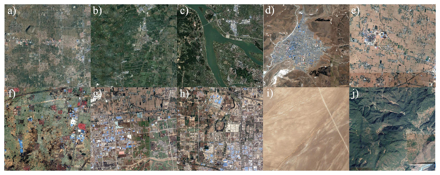
Figure 3Selected locations for data training (a–c) and data validation (d–j): (a) Baoding, (b) Shanghai, (c) GBA, and d) Nagqu, (e) Baoji, (f) Kaifeng, (g) Xi'an, (h) Zhengzhou, (i) Taklimakan Desert, and (j) Yunnan (© Google Earth).
Table 2Test results of selected locations for the blue-roof identification algorithm. NA – blue roofs are not available in the image.

∗ Training areas (only a subarea of its region).
Overall, 74 % to 88 % (hit rates) of the blue roof areas were successfully identified by the algorithm, while the false detection rates and false alarm rates ranged between 35 % and 51 % and between 0.1 % and 0.5 %, respectively. The low percentages of false alarm rates indicate only a small amount of non-blue-roof areas were included by the algorithm. A closer look at the results of false detection rates reveals that the false identification was mainly concentrated around the building boundaries because of the fuzziness of the building edges from the zoom level 14 satellite images. The percentages of false detection rates varied for images in different areas as the clearness of satellite images depended on the atmospheric conditions (e.g. cloudiness, air pollution) at the time they were taken. Compared with the images of Shanghai and GBA, the Baoding image has a relatively higher degree of blurriness which explained why the false detection rate for the Baoding was higher than those in the other two training areas. While the false selection around the building edges may incur different levels of errors to the blue-roof identification result, however, it does not generally affect the spatial distribution of the blue roof areas selected by the algorithm. It is observed that the GBA area has a low hit rate (i.e. 74 %) due to more scattered or isolated development than the other areas. In Boading and Shanghai, industrial parks are more common than in GBA. Buildings clustered together might have contributed to higher hit rates but at the same time caused high false detection rates, as the gap between buildings was also included as blue roof. To better evaluate the algorithm response to different environmental condition, another 7 areas (approximately 100 km2 each) covering a wide variety of geographical locations and features were selected to validate the blue-roof identification algorithm, as shown in Fig. 3d–j. The results in Table 2 show that the algorithm achieved 76 %–92 %, 9 %–54 %, and 0 %–0.3 % for the hit rates, false detection, and false alarm rates, respectively. These similar results found in Nagqu, Baoji, Kaifeng, Xi'an, and Zhengzhou indicate that the algorithm is relatively stable across the continent of China. For the remote areas in the Taklimakan Desert and Yunnan (Fig. 3i and j), it should be noted that the “ground truth” blue-roof areas were zero, so the hit rates were inapplicable for these two test images.
3.2 Blue-roof allocation process and CMAQ ready emission
A large amount of spatial data with various geospatial information (e.g. province shapefile) was processed through ArcGIS to create the gridded emissions for the CMAQ model. As mentioned, the selected blue-roof areas from the HSV algorithm have first undergone a spatial operation to remove the falsely identified water bodies from the blue-roof dataset. The data were then used to compute the gridded total blue-roof areas in each grid (see Fig. 4a). Furthermore, the total blue-roof areas in each province (i.e. Guangdong, Guangxi, and Jiangxi) within the domain were also generated. Figure 4b shows the province spatial surrogate (i.e. in Eq. 2) that was created for the GBA emission allocation. The values in each grid in the surrogate file should fall between 0 and 1, and the total in the province should sum up to 1.0 for data integrity. The yellow grids (values greater than 0) were clustered around the centre of PRD, reflecting that the high density of blue-roof buildings was identified along the Pearl River, and the yellow lines extended from PRD indicate that small remote industrial areas were built along the major highways in GBA. The grids with magenta (values with 0) were confirmed to be hilly areas, forests, or water reservoirs, and no blue-roof building was identified.

Figure 4(a) Snapshot of D3 (3 km) domain grids, and (b) calculated spatial surrogate.
Finally, to generate the final gridded industrial emissions, the spatial surrogate was applied to the MIX industrial emissions to spatially allocate the province-level emissions into the CMAQ grids. All sectoral emissions, including power, transportation, industrial, residential, agriculture, and others were aggregated together with the newly produced industrial emissions to generate the CMAQ ready gridded emissions for air quality simulation. Figure 5 shows the daily column total of CMAQ ready PM2.5 emissions (1 January 2015) for the base case, blue-roof case, and point- and area-based btmUp case from Zhang et al. (2020). In general, more spatial spread is observed in the blue-roof case than in the base case within the GBA area, but the spread is not as wide as in the point- and area-based btmUp case. The widespread PM2.5 emission in the btmUp case is attributed to the inclusion of both industrial point and industrial area sources, which was not applied the same way as in the base and blue-roof cases. In the base case (Fig. 5a), emission (over 200 g s−1 per grid of PM2.5) is intensely clustered around the city centres of Guangzhou (GZ) and Foshan (FZ). A circular belt of intense PM2.5 emission is observed along the coast of Zhujiang River Estuary in Shenzhen (SZ). In contrast, PM2.5 emission in the blue-roof case (Fig. 5b) is more widely spread across the region, with additional focuses in Dongguan (DG) and north of Zhongshan (ZS). The hotspots of PM2.5 exhibited in (Fig. 5b) are strongly aligned with the spatial pattern of hotspots from Cui et al. (2015), which was generated from the source apportionment method. In Shenzhen, the circular belt of high emission previously observed in the base case has disappeared. Further investigation shows that the coastal area along the Zhujiang River Estuary has already been converted into recreation and residential areas. Due to the high population density found in the area, the base case had allocated a large amount of PM2.5 emission to the area. For small industrial areas, the blue-roof case also seems to outperform the base case as it has identified more scattered industrial areas in the region. As shown in BE (Fig. 5), the blue-roof method is capable of capturing the small industrial towns (see Fig. S1 in the Supplement) along the major highways. For this particular example, the industrial area captured by the blue-roof method is located in the rural area of Qingyuan with over 20 petrochemical factories or warehouses, which were missed in the base case. When comparing the blue-roof case with the point- and area-based btmUp case (Fig. 5c), clear spots of PM2.5 underestimation were observed which are shown in the square boxes of Fig. 5b pointing at the northeastern and southwestern sides of PRD, and north of Guangzhou. The focus of the study is to investigate the improvement of the blue-roof surrogate in the MIX industrial sector, rather than the performance differences between the MIX unified emissions and local bottom-up emissions. Therefore, instead of showing the uncertainty of emission inventory, which is infeasible here, we have developed a spatial blue-roof surrogate (Fig. 4b), the comparison of the model-ready emissions (Fig. 5), and the time series plots of typical stations (Fig. 7) to illustrate the performance of the blue-roof algorithm.

Figure 5Daily column total of PM2.5 emission from D3 (3 km) domain: (a) base case, (b) blue-roof case, and (c) point- and area-based btmUp case. Note: blue arrows indicate Foshan (FS), Guangzhou (GZ), Shenzhen (SZ), Dongguan (DG), Zhongshan (ZS), and BE (blue-roof example). Boxes indicate the locations with large spatial differences between the blue-roof and the btmUp cases.
3.3 CMAQ-simulated air quality and statistical comparison
3.3.1 Performance comparison between the base case and blue-roof case
The CMAQ simulation was performed on both base case and blue-roof case to evaluate the air quality impacts of using different allocation methods for industrial emissions. In addition, to better understand how well the blue-roof method performs, the CMAQ results using the local point- and area-based btmUp emission method adopted from Zhang et al. (2020) were also included in the comparison. Figure 6 shows the simulated monthly average surface PM2.5 for the base case (panels a, d), blue-roof case (panels b, e), and point- and area-based btmUp case (panels c, f); the left (panels a–c) and right (panels d–f) panels represent the January and August cases, respectively. As expected, the base case (panels a, d) has much lower spatial spread when compared with the blue-roof (panels b, e) and the point- and area-based btmUp (panels c, f) cases illustrated in the earlier section. The wider spreading of PM2.5 in the blue-roof case (panels b, e) was attributed to the redistribution of industrial emissions from highly populated areas (i.e. Guangzhou, Foshan, and Shenzhen) found in the base case into other areas of GBA. The redistribution process has lowered the CMAQ prediction for those three urban areas, moreover, to reduce the PM2.5 prediction along the coast of Zhujiang River Estuary at the circular belt of Shenzhen, which was mentioned in Fig. 5a. As monsoon wind moves differently in summer and winter, it affects the regional pollutant transport and air quality prediction in the GBA area. For the winter case, with the effect of the northeast prevailing wind in January, the reduction of Guangzhou and Foshan emissions and pollution (See Fig. S2) has a strong positive impact on both local and downwind regions (i.e. south of Guangzhou – Zhongshan, Zhuhai, and Macau). This is illustrated by the PM2.5 time-series plot of Zhongshan station (22∘31′16.0′′ N 113∘22′36.8′′ E) shown in Fig. 7a) where the large PM25 overestimation in the base case (grey line) was significantly reduced into the more acceptable range shown in the blue-roof case (blue line). The root mean square error (RMSE) was trimmed down by nearly half to about 23.0 µg m−3 (from 49.2 µg m−3 in the base case to 26.2 µg m−3 in the blue-roof case), demonstrating the effectiveness of using the blue-roof allocation method in the top-down emission approach. This is not entirely the same case for summer (August) when the prevailing wind is from the southwest and brings a clean marine boundary to the region. Although, in some situations, due to the presence of distant typhoon (e.g. Soudelor, 4–11 August, and Goni, 21–25 August), the outermost typhoon circulation had forced the wind direction to change to northeasterly and resulted in a similar transport phenomenon that caused the PM2.5 spikes in summer (Lam et al., 2018). For the general situation during the non-typhoon conditions, stronger PM2.5 underestimation is observed in the blue-roof case than in the base case, worsening the mean bias (MB) from −7.0 in the base case to −12.4 µg m−3 in the blue-roof case. In terms of RMSE, there is nearly no difference between the base case (i.e. 20.47 µg m−3) and blue-roof case (i.e. 20.48 µg m−3), as the performance degradation observed during the non-typhoon period was compensated by the improvement during the typhoon period. Figure 8 shows the comparison of spatial performance between the base and blue-roof cases. The “RMSE improvement” means that the blue-roof case has outperformed the base case (RMSEblue-roof case − RMSEbase case < 0), while the “RMSE impact” means that the blue-roof case has worsened the CMAQ performance (RMSEblue-roof case − RMSEbase case ≥ 0). In general, the majority of stations in Guangzhou, Foshan, and Dongguan have received a substantial improvement in both January and August, as shown in yellow colour, while some outer stations in the southern and eastern parts of PRD and Hong Kong get worse (i.e. RMSE impact), shown in red colour. These stations with the “RMSE impact” designation are primarily suburban areas where a mixed land-use pattern was identified. Overall, stations with “RMSE improvement” yield an average RMSE of 45.8 and 30.6 µg m−3 for the base and blue-roof cases in January, respectively, which translates to about −12.3 µg m−3 for the RMSE improvement. This number is much larger than +0.7 µg m−3 in magnitude obtained from the group with the “RMSE impact” designation, which illustrates the improvement has outweighed the impact. For August, the differences in RMSE(blue-roof case − base case) under the “RMSE improvement” and “RMSE impact” are −4.5 and +0.73 µg m−3, respectively. Although there are quite a number of stations (∼ 25+) falling into the category of “RMSE impact”, their actual RMSE differences are relatively small (e.g. ∼ 75 % of stations with RMSE less than 1 µg m−3). Hence, it does not cause any concern for the blue-roof method. Detailed statistical results for each station have been incorporated into Tables S1 and S2, and the corresponding station locations are available in Fig. S3.

Figure 6CMAQ-predicted monthly surface PM2.5: (a) January base case, (b) January blue-roof case, (c) January point- and area-based btmUp case, (d) August base case, (e) August blue-roof case, and (f) August point- and area-based btmUp case.
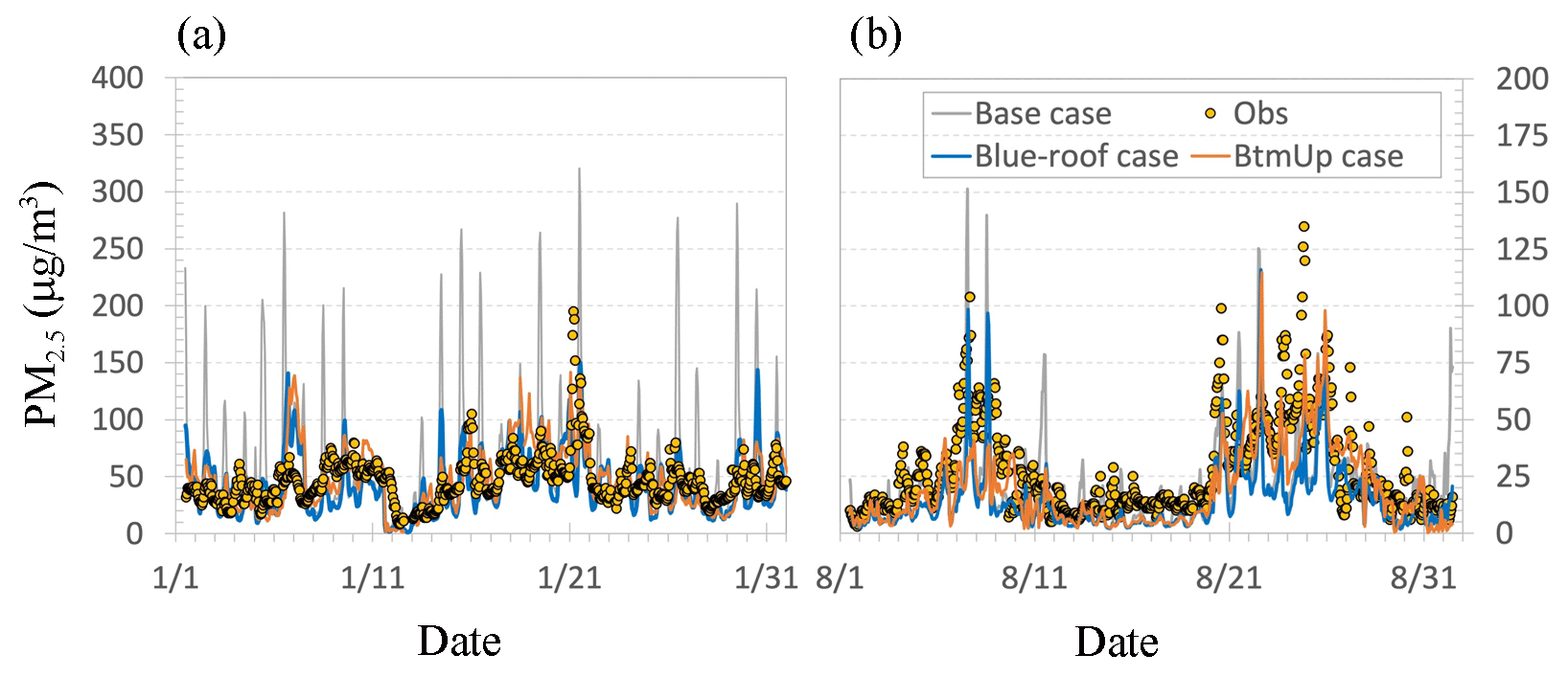
Figure 7Time series of PM2.5 at station CN_1379A (22∘31′16.0′′ N, 113∘22′36.8′′ E) – Zhongshan: (a) January and (b) August.
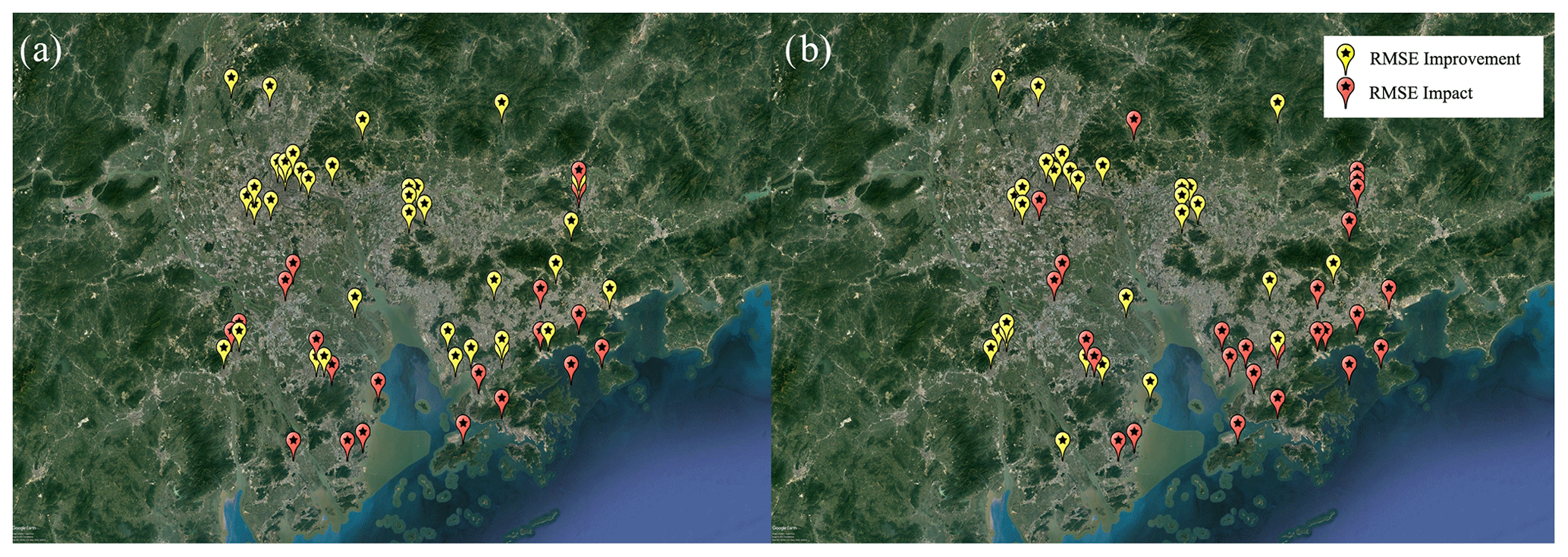
Figure 8Spatial comparison of RMSE performance between the base case and blue-roof case: (a) January and (b) August. Stations with yellow colour indicates “RMSE improvement” where the RMSE of the blue-roof case is lower than the RMSE of the base case (RMSEblue-roof case − RMSEbase case < 0). Stations with red colour refer to “RMSE impact” (RMSEblue-roof case − RMSEbase case ≥ 0), meaning that the situation gets worse after using the blue-roof algorithm (© Google Earth).
3.3.2 Performance comparison between the blue-roof case and point- and area-based btmUp case
It is essential to evaluate the performance of the blue-roof case using observations, while it is also interesting to investigate the difference between the performance of the blue-roof allocation method and the local point- and area-based bottom-up method using relatively fine resolution (i.e. 3 km). In general, the CMAQ-simulated PM2.5 using the blue-roof method (Fig. 6b and e) has shown a lower spatial spread than the one using the point- and area-based btmUp approach (bottom panel of Fig. 6). The low spread of PM2.5 in the blue-roof case may be attributed to the insufficient separation of existing industrial emissions. As the blue-roof emission approach took all industrial emissions and treated them as location-based emissions without assigning any portion of them to area source, the lack of the representation of industrial area sources (e.g. fugitives) in the inventory may have resulted in a less spatial spread, as shown in Fig. 5b. Moreover, the base unit of industrial emissions in the current approach is “province-level”, which is insufficient to distinguish the industrial speciality for different cities or counties within the domain. From the time-series analysis shown in Fig. 7a and b, the RMSE performance of the blue-roof case (blue line) is quite comparable with the point- and area-based btmUp case (orange line) and observations (yellow dots). This particular example of the blue-roof case (Fig. 7b) can even outperform the point- and area-based btmUp case in predicting PM2.5. From Tables S1 and S2, the average RMSE in January (August) for the base, blue-roof and btmUp cases are 44.8 (25.7), 33.3 (22.4), and 27.8 (18.3) µg m−3, respectively. This illustrates the blue-roof case has outperformed the base case but still is not as good as the local point- and area-based btmUp case. Figure 9 shows the PM2.5 performance of different station types (see Fig. S3). As expected, the point- and area-based btmUp case has the lowest RMSE among the cases for all station types, while there is a clear improvement of RMSE in urban stations in the blue-roof case; implementing the blue-roof method has eliminated some of the extreme outliers from the base case, forming a much more narrowed RMSE range. In terms of rural and suburban stations, minor RMSE improvements (i.e. mean values) have been observed. It should be noted that the wider RMSE range showed in the blue-roof case (as compared with the base case) for the suburban category in Fig. 9a is just a visual illusion. The maximum RMSE value of the base case in the suburban category has been plotted as an outlier (dot) instead of a regular line in the upper whisker. Hence, the RMSE range (the two-end whiskers) in the blue-roof case is visually taller than the one in the base case. Figure S4 shows the station (i.e. CN_1352A) that corresponds to the maximum RMSE in the suburban category, and better performance has been obtained from the blue-roof case (blue line). In the station, the RMSEs in January (August) for the base and blue-roof cases are 84.4 (36.0) and 50.0 (27.5) µg m−3, respectively.

Table 3Summary of performance statistics in the case study.
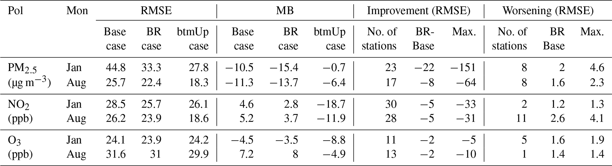
Note – Pol: pollutant; Mon: month; BR: blue-roof case; RMSE: root mean square error; MB: mean bias; Max: maximum. The RMSE sections on the right only reflect the number of stations that have RMSE changes greater than ±1.
3.3.3 Performance of other air pollutants
Finally, to better understand the overall impacts on local air quality prediction, Table 3 shows the comparison of performance statistics among the base case, blue-roof case, and point- and area-based btmUp case for PM2.5, NO2, and O3. In general, all three pollutants received some improvements when switching from the population-based method to the blue-roof allocation method. A more significant improvement of RMSE is observed in PM2.5 and NO2, which ranges from 3.3–11.5 µg m−3 for PM2.5 and 2.3–2.7 ppb for NO2. The result is somewhat expected as industrial sector is the largest contributor of PM2.5 and NO2 emissions in the MIX inventory. In terms of MB, slight degradation is observed in PM2.5, which may either be caused by the slight underestimation of total PM2.5 emission in GBA or insufficient generation of secondary organic PM2.5 from CMAQ, which is commonly observed in version 5.02. For NO2, a slight improvement is observed, which resulted from the removal of large overestimations in the city centres of GZ, FZ, and SZ. Among 75 observation stations, on average, 25 stations received an improvement in RMSE for PM2.5 and NO2. The largest RMSE improvement is observed in the Foshan area with −151 µg m−3 improvement in PM2.5 (See Fig. S2) and 33 ppb in NO2. This result clearly reflects the weakness and limitation of the population-based method for industrial allocation in the fine-resolution grid. In some stations (i.e. seven), higher RMSEs (i.e. an average of 1.8 µg m−3 for PM2.5 and 1.9 ppb for NO2) are observed. For ozone, a minor improvement (i.e. 0.2 and 0.6 ppb in RMSE) has been found which may be attributed to the improvement in NO2 prediction and consequently affect the NOx titration process in ozone chemistry. As the improvement is at a marginal level, it is concluded that the improvement is limited.
When comparing the blue-roof case with the local point- and area-based btmUp case, a lower RMSE of PM2.5 has been observed in the blue-roof case (Table 3). The difference in the RMSE reflects that there is still room for improvement in the blue-roof method. From the large negative MB observed in the MIX emission cases of PM2.5, one suggestion would be to scale up the sectorial PM2.5 totals from the MIX inventory using an inverse modelling approach (e.g. satellite inversion or source apportionment), which may lead to a better initial PM2.5 emission for CMAQ modelling. In terms of NO2 and O3, comparable results (i.e. RMSE) are obtained between the blue-roof and point- and area-based btmUp cases. Although there is slightly higher RMSE (23.9 ppb vs. 18.6 ppb in August) in one of the blue-roof cases, in general, they all fall within a similar range of values. In terms of MB, the values in the blue-roof case vary across the seasons, with positive MB of NO2 and negative MB of O3 in January, and positive MB of both NO2 and O3 in August. For the point- and area-based btmUp case, negative MB has been observed in both January and August. Among the seasons, it is noted that reducing NO2 emission in the blue-roof case in January may improve the MB of both NO2 and O3 as it reduces the NO2 titration effect in the ozone formation process and causes higher ozone. However, since the MBs (i.e. 3 to 5 ppb) of NO2 are relatively small (as compared with the MB of PM2.5, −10 to −15 µg m−3), no NO2 adjustment is recommended.
In this work, we developed a new method called the “blue-roof allocation method” for assigning industrial emissions for the gridded air quality simulation. The proposed method not only provides an alternative way of handling Chinese industrial emissions from the existing population-based method but also allows a higher resolution (up to 3 km) to be generated for local air quality study. As the rapid urban redevelopment and mature public transportation network (e.g. metro/train system) were emerging in China, the relationship of proximity between living place and the workplace was slowly diminished. Hence, the traditional method using population density as a spatial proxy for industrial emissions has become obsolete.
In the blue-roof allocation method, satellite images from zoom level 14 were applied as the basis for blue-roof extraction. An HSV colour detection algorithm was developed and trained to carry out blue-roof identification. The captured blue-roofs were then converted and stored as individual polygons for further processing. The sequence of ArcGIS subprocesses was applied to generate spatial surrogate and gridded emissions. The gridded emissions were tested with CMAQ air quality simulations for January and August of 2015. The results show that large improvements are observed in both PM2.5 and NO2 predictions when compared with the traditional method (i.e. population-based method). By using the blue-roof method, not only were the emission errors from large metropolitan areas reduced, but also the emissions from scattered industrial areas located in the rural area were accurately captured. The emission allocation using the blue-roof method has decluttered the urban emissions, allowing better spread across the region. We are confident that the new method is capable of generating high-resolution input (up to 3 km) for local air quality modelling and yielding reasonable air quality results. Please be aware that the assumption of the blue-roof method that larger blue roofs have more emissions may not always be sufficient under different resolutions. Therefore, further increasing the spatial resolution to lower than 3 km (e.g. 1 km) should be performed with caution. Before the point- and area-based bottom-up approach with the unit process data is fully available in China, this method will be a useful technique for handling industrial emissions in China.
The simulated output is available from the corresponding author on reasonable request.
The supplement related to this article is available online at: https://doi.org/10.5194/acp-21-12895-2021-supplement.
The main contributions to model simulation and data management were made by YFL, CCC, and XZ and to the data analyses by YFL, CCC, and XZ. The study was conceptualized by YFL and JSF. All co-authors prepared the original draft of the paper. Resources were organized by YFL and JCHF.
The authors declare that they have no conflict of interest.
Publisher’s note: Copernicus Publications remains neutral with regard to jurisdictional claims in published maps and institutional affiliations.
This article is part of the special issue “Regional assessment of air pollution and climate change over East and Southeast Asia: results from MICS-Asia Phase III”. It is not associated with a conference.
The authors would like to acknowledge Willy Ying, Sairy Wang, and Stephen Chan for their supports in the research and the Hong Kong Environmental Protection Department for providing emission inputs. The computations were partially performed using research computing facilities offered by Information Technology Services, the University of Hong Kong.
This research has been supported by the Innovation and Technology Fund (grant no. ITS/099/16FX) and the Research Grants Council University Grants Committee (grant no. 21300214).
This paper was edited by Qiang Zhang and reviewed by two anonymous referees.
Athanasopoulou, E., Tombrou, M., Pandis, S. N., and Russell, A. G.: The role of sea-salt emissions and heterogeneous chemistry in the air quality of polluted coastal areas, Atmos. Chem. Phys., 8, 5755–5769, https://doi.org/10.5194/acp-8-5755-2008, 2008.
Chen, L., Gao, Y., Zhang, M., Fu, J. S., Zhu, J., Liao, H., Li, J., Huang, K., Ge, B., Wang, X., Lam, Y. F., Lin, C.-Y., Itahashi, S., Nagashima, T., Kajino, M., Yamaji, K., Wang, Z., and Kurokawa, J.: MICS-Asia III: multi-model comparison and evaluation of aerosol over East Asia, Atmos. Chem. Phys., 19, 11911–11937, https://doi.org/10.5194/acp-19-11911-2019, 2019.
Cui, H., Chen, W., Dai, W., Liu, H., Wang, X., and He, K.: Source apportionment of PM2.5 in Guangzhou combining observation data analysis and chemical transport model simulation, Atmos. Environ., 116, 262–271, https://doi.org/10.1016/j.atmosenv.2015.06.054, 2015.
Du, Y.: New Consolidation of Emission and Processing for Air Quality Modeling Assessment in Asia, Master thesis, Department of Civil and Environmental Engineering, University of Tennessee, Knoxville, TN, USA, 2008.
ECCC: Canada–United States Air Quality Agreement: progress report 2016, Environment and Climate Change Canada, Gatineau, QC, Canada, 2017.
Giglio, L., Randerson, J. T., and van der Werf, G. R.: Analysis of daily, monthly, and annual burned area using the fourth-generation global fire emissions database (GFED4), J. Geophys. Res.-Biogeo., 118, 317–328, https://doi.org/10.1002/jgrg.20042, 2013.
Giuliano, G. and Small, K. A.: Is the Journey to Work Explained by Urban Structure?, Urban Studies, 30, 1485–1500, https://doi.org/10.1080/00420989320081461, 1993.
HKEPD: Regional Air Quality Modelling System (PATH) – Feasibility Study, ENVIRON Hong Kong Limited, Hong Kong SAR, China, 2011.
HKEPD: Guangdong-Hong Kong-Macao Pearl River Delta Regional Air Quality Monitoring Network: A Report of Monitoring Results in 2015, Environmental Protection Department, Hong Kong SAR, China, 2016.
HKEPD: Air Quality Objectives (AQO) Review Working Group – Annex C Air Science and Health Sub-group, Hong Kong Environmental Protection Department, Hong Kong SAR, China, 2019.
Janssens-Maenhout, G., Crippa, M., Guizzardi, D., Dentener, F., Muntean, M., Pouliot, G., Keating, T., Zhang, Q., Kurokawa, J., Wankmüller, R., Denier van der Gon, H., Kuenen, J. J. P., Klimont, Z., Frost, G., Darras, S., Koffi, B., and Li, M.: HTAP_v2.2: a mosaic of regional and global emission grid maps for 2008 and 2010 to study hemispheric transport of air pollution, Atmos. Chem. Phys., 15, 11411–11432, https://doi.org/10.5194/acp-15-11411-2015, 2015.
Krzyzanowski, J.: The Importance of Policy in Emissions Inventory Accuracy – A Lesson from British Columbia, Canada, J. Air Waste Manage. Assoc., 59, 430–439, https://doi.org/10.3155/1047-3289.59.4.430, 2009.
Kurokawa, J., Ohara, T., Morikawa, T., Hanayama, S., Janssens-Maenhout, G., Fukui, T., Kawashima, K., and Akimoto, H.: Emissions of air pollutants and greenhouse gases over Asian regions during 2000–2008: Regional Emission inventory in ASia (REAS) version 2, Atmos. Chem. Phys., 13, 11019–11058, https://doi.org/10.5194/acp-13-11019-2013, 2013.
Lam, Y. F. and Fu, J. S.: Corrigendum to “A novel downscaling technique for the linkage of global and regional air quality modeling” published in Atmos. Chem. Phys., 9, 9169–9185, 2009, Atmos. Chem. Phys., 10, 4013–4031, https://doi.org/10.5194/acp-10-4013-2010, 2010.
Lam, Y.-F., Davis, W. T., Miller, T. L., and Fu, J. S.: System enhancement of title V permit reviews and point source inventories, Proceedings of the A&WMA's 97th Annual Conference & Exhibition, 22–25 June 2004, Indianapolis, IN, USA, 1673–1679, 2004.
Lam, Y. F., Cheung, H. M., and Ying, C. C.: Impact of tropical cyclone track change on regional air quality, Sci. Total Environ., 610–611, 1347–1355, https://doi.org/10.1016/j.scitotenv.2017.08.100, 2018.
Li, M., Zhang, Q., Kurokawa, J.-I., Woo, J.-H., He, K., Lu, Z., Ohara, T., Song, Y., Streets, D. G., Carmichael, G. R., Cheng, Y., Hong, C., Huo, H., Jiang, X., Kang, S., Liu, F., Su, H., and Zheng, B.: MIX: a mosaic Asian anthropogenic emission inventory under the international collaboration framework of the MICS-Asia and HTAP, Atmos. Chem. Phys., 17, 935–963, https://doi.org/10.5194/acp-17-935-2017, 2017.
Li, M., Zhang, Q., Zheng, B., Tong, D., Lei, Y., Liu, F., Hong, C., Kang, S., Yan, L., Zhang, Y., Bo, Y., Su, H., Cheng, Y., and He, K.: Persistent growth of anthropogenic non-methane volatile organic compound (NMVOC) emissions in China during 1990–2017: drivers, speciation and ozone formation potential, Atmos. Chem. Phys., 19, 8897–8913, https://doi.org/10.5194/acp-19-8897-2019, 2019.
Liu, S. H., Li, X. B., and Zhang, M.: Scenario Analysis on Urbanization and Rural – Urban Migration in China, Institute of Geographic Sciences and Natural Resources Research, Chinese Academy of Sciences, Beijing, China, 2003.
Ng, S. K. W., Lin, C., Chan, J. W. M., Yip, A. C. K., Lau, A. K. H., and Fung, J. C. H.: Study on Marine Vessels Emission Inventory, The Environmental Protection Department The HKSAR Government, Hong Kong SAR, China, 2012.
Ohara, T., Akimoto, H., Kurokawa, J., Horii, N., Yamaji, K., Yan, X., and Hayasaka, T.: An Asian emission inventory of anthropogenic emission sources for the period 1980–2020, Atmos. Chem. Phys., 7, 4419–4444, https://doi.org/10.5194/acp-7-4419-2007, 2007.
Streets, D. G., Bond, T. C., Carmichael, G. R., Fernandes, S. D., Fu, Q., He, D., Klimont, Z., Nelson, S. M., Tsai, N. Y., Wang, M. Q., Woo, J.-H., and Yarber, K. F.: An inventory of gaseous and primary aerosol emissions in Asia in the year 2000, J. Geophys. Res.-Atmos., 108, 8809, https://doi.org/10.1029/2002jd003093, 2003.
Tan, J., Fu, J. S., Dentener, F., Sun, J., Emmons, L., Tilmes, S., Sudo, K., Flemming, J., Jonson, J. E., Gravel, S., Bian, H., Davila, Y., Henze, D. K., Lund, M. T., Kucsera, T., Takemura, T., and Keating, T.: Multi-model study of HTAP II on sulfur and nitrogen deposition, Atmos. Chem. Phys., 18, 6847–6866, https://doi.org/10.5194/acp-18-6847-2018, 2018.
Yang, J.: Transportation Implications of Land Development in a Transitional Economy: Evidence from Housing Relocation in Beijing, Transp. Res. Record, 1954, 7–14, https://doi.org/10.1177/0361198106195400102, 2006.
Zhang, X.: Numerical Model Sensitivity Analysis and the Three-dimensional Variational Data Fusion Approach for Optimizing Air Quality Modeling, PhD thesis, Division of Environment and sustainability, Hong Kong University of Science and Technology, Hong Kong SAR, China, 2020.
Zhang, X., Fung, J. C. H., Zhang, Y., Lau, A. K. H., Leung, K. K. M., and Huang, W.: Assessing PM2.5 emissions in 2020: The impacts of integrated emission control policies in China, Environ. Pollut., 263, 114575–114575, https://doi.org/10.1016/j.envpol.2020.114575, 2020.
Zhang, X., Fung, J. C. H., Lau, A. K. H., Hossain, M. S., Louie, P. K. K., and Huang, W.: Air quality and synergistic health effects of ozone and nitrogen oxides in response to China's integrated air quality control policies during 2015–2019, Chemosphere, 268, 129385, https://doi.org/10.1016/j.chemosphere.2020.129385, 2021.
Zhao, S., Bi, X., Zhong, Y., and Li, L.: Chinese Industrial Park Planning Strategies Informed by American Edge Cities' Development Path – Case Study of China (Chongzuo)-Thailand Industrial Park, Procedia Engineer., 180, 832–840, https://doi.org/10.1016/j.proeng.2017.04.244, 2017.
Zhao, Y., Qiu, L. P., Xu, R. Y., Xie, F. J., Zhang, Q., Yu, Y. Y., Nielsen, C. P., Qin, H. X., Wang, H. K., Wu, X. C., Li, W. Q., and Zhang, J.: Advantages of a city-scale emission inventory for urban air quality research and policy: the case of Nanjing, a typical industrial city in the Yangtze River Delta, China, Atmos. Chem. Phys., 15, 12623–12644, https://doi.org/10.5194/acp-15-12623-2015, 2015.
Zheng, B., Tong, D., Li, M., Liu, F., Hong, C., Geng, G., Li, H., Li, X., Peng, L., Qi, J., Yan, L., Zhang, Y., Zhao, H., Zheng, Y., He, K., and Zhang, Q.: Trends in China's anthropogenic emissions since 2010 as the consequence of clean air actions, Atmos. Chem. Phys., 18, 14095–14111, https://doi.org/10.5194/acp-18-14095-2018, 2018.