the Creative Commons Attribution 4.0 License.
the Creative Commons Attribution 4.0 License.
 | 17 Aug 2021
Understanding the model representation of clouds based on visible and infrared satellite observations
Stefan Geiss
Leonhard Scheck
Alberto de Lozar
Martin Weissmann
There is a rising interest in improving the representation of clouds in numerical weather prediction models. This will directly lead to improved radiation forecasts and, thus, to better predictions of the increasingly important production of photovoltaic power. Moreover, a more accurate representation of clouds is crucial for assimilating cloud-affected observations, in particular high-resolution observations from instruments on geostationary satellites. These observations can also be used to diagnose systematic errors in the model clouds, which are influenced by multiple parameterisations with many, often not well-constrained, parameters. In this study, the benefits of using both visible and infrared satellite channels for this purpose are demonstrated. We focus on visible and infrared Meteosat SEVIRI (Spinning Enhanced Visible InfraRed Imager) images and their model equivalents computed from the output of the ICON-D2 (ICOsahedral Non-hydrostatic, development version based on version 2.6.1; Zängl et al., 2015) convection-permitting, limited area numerical weather prediction model using efficient forward operators. We analyse systematic deviations between observed and synthetic satellite images derived from semi-free hindcast simulations for a 30 d summer period with strong convection. Both visible and infrared satellite observations reveal significant deviations between the observations and model equivalents. The combination of infrared brightness temperature and visible reflectance facilitates the attribution of individual deviations to specific model shortcomings. Furthermore, we investigate the sensitivity of model-derived visible and infrared observation equivalents to modified model and visible forward operator settings to identify dominant error sources. Estimates of the uncertainty of the visible forward operator turned out to be sufficiently low; thus, it can be used to assess the impact of model modifications. Results obtained for various changes in the model settings reveal that model assumptions on subgrid-scale water clouds are the primary source of systematic deviations in the visible satellite images. Visible observations are, therefore, well-suited to constrain subgrid cloud settings. In contrast, infrared channels are much less sensitive to the subgrid clouds, but they can provide information on errors in the cloud-top height.
- Article
(9500 KB) - Full-text XML
- BibTeX
- EndNote


As the share of renewable energy in the world's total electricity supply is rising, there is an increased need to improve cloud and radiation forecasts. Solar photovoltaic (PV) power production is one of the fastest-growing forms of renewable energy, with a global increase of 22 % in 2019 (IEA, 2020). It will soon become challenging to integrate PV power with its strong weather-related fluctuations into the electricity grid. Therefore, a more accurate prediction of renewable power generation based on numerical weather prediction (NWP) models is important to maintain network safety and allow for the efficient usage of alternative power sources (Tuohy et al., 2015). The output power of a photovoltaic power plant is mainly determined by solar irradiance, which in turn is mainly affected by cloud cover (Zack, 2011). According to Köhler et al. (2017), the main shortcomings of NWP in this context are related to the prediction of low stratus and fog, the spatial and temporal resolution of convection, shallow cumulus, and Saharan dust outbreaks. Kurzrock et al. (2018) also demonstrated that clouds, in particular the representation of low stratus in the model, dominate the uncertainty of PV power production. Advances in the prediction of clouds, radiation and PV power generation are possible by improving the representation of clouds in NWP models; this can be achieved by including more accurate physical parameterisations or tuning existing parameterisations related to clouds.
Moreover, a good representation of clouds in NWP models is also a prerequisite for assimilating cloud-related observations, which improves the initial state from which forecasts are started and, thus, also subsequent forecasts. Cloud-related observations like satellite images in the solar or thermal spectrum can only be assimilated if observed and simulated clouds exhibit a similar climatology. Unfortunately, this is not necessarily the case in current NWP systems (Gustafsson et al., 2018; Tuohy et al., 2015). Therefore, understanding and mitigating these systematic deviations will be an essential ingredient for the operational assimilation of such observations. Some studies have already shown the benefit of assimilating cloud-affected satellite radiances in the infrared (e.g. Geer et al., 2018; Honda et al., 2018) and in the visible (Scheck et al., 2020) in experimental set-ups or idealised experiments (Schröttle et al., 2020). The assimilation led to significant improvements in cloud-related quantities and dynamical variables, as clouds are often associated with meteorologically sensitive areas (atmospheric instability) (McNally, 2002). However, current convection-permitting regional NWP systems still do not assimilate cloud-affected satellite observations (Gustafsson et al., 2018), mainly due to systematic deviations.
Cloud-related observations can also be used to diagnose systematic errors in the model clouds and get information on which processes or parameterisations in the model need to be improved. Satellite images obtained by instruments on geostationary or polar-orbiting satellites are well-suited for this purpose, as they contain high-resolution information on the location and properties of clouds. As discussed in more detail in Sect. 2.2, the solar and thermal channels of these instruments provide complementary information on clouds' properties and can also depend, often in an ambiguous way, on the thermodynamic state of the atmosphere, aerosols and trace gases. In prior model evaluation studies, the satellite radiance has often not been used, with researchers instead opting for easier to interpret quantities like cloud fraction, cloud optical depth, and the cloud-top height derived from them using retrieval algorithms (e.g. Zhang et al., 2005; Otkin and Greenwald, 2008; Senf et al., 2020). These retrieved quantities correspond directly to model variables or are closely connected to them. The combination of information derived from visible and infrared satellite observations like in the ISCCP (International Satellite Cloud Climatology Project; see e.g. Rossow and Schiffer, 1991) approach that constructs cloud type histograms of retrieved cloud optical thickness and cloud-top pressure has been particularly helpful for detecting shortcomings related to model clouds (e.g. Tselioudis and Jakob, 2002; Otkin and Greenwald, 2008; Franklin et al., 2013). These studies have shown that systematic cloud biases are present in most models and that the representation of clouds depends on nearly every parameterisation in the model (Webb et al., 2001).
While quantities retrieved from satellite observations like cloud optical depth are easier to interpret than the observations themselves, they have the drawback that characterising their errors is often problematic (Errico et al., 2007). Inter alia, retrievals often incorporate model information leading to error correlations between the model and the retrieved information used for evaluation. Therefore, in data assimilation, the “direct assimilation” of observations by means of forward operators is generally preferred over the assimilation of retrievals. A reasonable characterisation of errors is crucial not only for data assimilation but also for model evaluation. Reliable conclusions can be drawn about model errors if the errors in the evaluation method are sufficiently small.
The aim of this study is to demonstrate the benefits of evaluating the representation of clouds in NWP models using a combination of visible and infrared satellite images. Our results are based on simulations with the ICON-D2 (ICOsahedral Non-hydrostatic, development version based on version 2.6.1; Zängl et al., 2015) preoperational convection-permitting model of the Deutscher Wetterdienst (DWD; German Meteorological Service) for a highly convective summer period of 30 d over Germany and neighbouring areas. We will show that better insights into the origin of the systematic cloud errors can be gained using the two different satellite channels. Moreover, it will be demonstrated that this approach is also useful for assessing the impact of model changes aimed at reducing errors in the clouds and can, thus, directly support model tuning efforts.
Given the advantages related to error characterisation, we will follow the forward operator approach in this study and compare observed and synthetic images. For the generation of synthetic infrared images, we will rely on the fast methods available in the RTTOV (Radiative Transfer for TOVS) radiative transfer package (Saunders et al., 2018), which is operationally used by many weather centres (e.g. the European Centre for Medium-Range Weather Forecasts). Several authors have examined the related uncertainties of these methods (e.g. Senf and Deneke, 2017; Saunders et al., 2017, 2018). For visible channels, we apply the newly developed VISible satellite image Forward OPerator (VISOP), which is based on the Method for Fast Satellite Image Synthesis (MFASIS) 1D radiative transfer method (Scheck et al., 2016) and an extension to account for the most important 3D radiative transfer (RT) effects (Scheck et al., 2018). The uncertainties of the visible forward operator will be discussed in this study.
The remainder of the paper is structured as follows: the experimental set-up is presented in Sect. 2. Two selected days with clouds on different levels are analysed in Sect. 3 to introduce satellite observations and their characteristics. This is followed by a discussion of the cloud statistics for a full test period and associated systematic deviations. In Sect. 4, we assess the sensitivity of synthetic satellite images to model and visible operator settings. For visible reflectances, forward operator uncertainties and model sensitivity are compared. Conclusions are provided in Sect. 5.
2.1 Model set-up and sensitivity experiments
To evaluate the cloud statistics during this period, we use the preoperational convection-permitting ICON-D2 (ICOsahedral Non-hydrostatic, development version based on version 2.6.1; Zängl et al., 2015) model configuration with prescribed lateral boundary conditions (BCs) and a one-way nesting. ICON-D2 replaced the operational COSMO-D2 (Consortium for Small scale-Modelling with a grid spacing of 2.2 km) model (Baldauf et al., 2018). Simulations over Germany (Fig. 1) with a horizontal grid spacing of 2.1 km and 65 vertical levels are initialised once on 26 May 2016 at 00:00 UTC from downscaled ICON-EU analysis initial conditions. ICON-EU analysis BCs drive this semi-free simulation with an hourly update and a forecast horizon of 30 d. The simulation period and domain size are sufficiently large for the atmospheric model to develop its own cloud distribution without perturbations from data assimilation or nudging. In our reference simulation, the operational single-moment bulk microphysical parameterisation accounting for water vapour (qv), cloud water (qc), cloud ice (qi), snow (qs), rain (qr) and graupel (qg) is used (Lin et al., 1983; Reinhardt and Seifert, 2006).

Figure 1ICON-D2 domain in the observation space (grey shading) and the reduced evaluation domain (red box). The orange x symbols indicate the DWD pyranometer stations that measure global horizontal irradiance.
The reference preoperational model configuration has been reached through extensive tuning of many parameters whose values are uncertain. As many of these parameterisations are related to clouds, it would be very beneficial if such parameterisations could be further constrained by satellite observations. For this reason, we examine the sensitivity of solar reflectances and infrared brightness temperatures (BTs) to variations in cloud-related parameterisations. We performed six additional simulations in which cloud-related parameterisations were modified within their range of uncertainty, i.e. using perturbed values that are physically plausible. For this purpose, we modified the following four parameterisations:
-
The cloud droplet number concentration in ICON is used to calculate the cloud optical properties and the onset of precipitation. ICON employs the parameterisation of Segal and Khain (2006), which determines how many droplets are in a cloud depending on an aerosol number concentration derived from the climatology and on an updraught velocity at nucleation. The determination of the updraught velocity in a 2km resolution model is not straightforward because updraughts are under-resolved. ICON assumes a constant updraught velocity, which serves as a control parameter: the number of nucleated droplets increases with the updraught velocity.
-
The turbulent subgrid-scale cloud parameterisation determines the cloud cover due to the unresolved variability in the model. The resulting turbulent cloud cover ccturb is combined with the detrainment cloud cover, which is given by a diagnostic approximation of the equivalent term in Tiedtke (1993). We focus on the turbulent parameterisation of liquid clouds, as those are the main source of subgrid-scale clouds in the summer period chosen for the experiments.
The turbulent cloud parameterisation in ICON for liquid clouds is based on the assumption of an asymmetric probability distribution function (PDF) of total water (including liquid and vapour). The cloud-cover function that is used starts from this assumption, but it has been empirically modified based on global and regional experiments (Martin Köhler, DWD, personal communication, 2020). The final function reads
where Δq is the variance of the total-water PDF and is determined by the turbulence scheme; A and B are tunable parameters that are described below; and qsat is the water vapour at saturation using the mean temperature and pressure in the grid box. Some limiters and resolution-dependent corrections are then applied to achieve the final cloud fraction, but their description is not relevant for this paper.
The parameter A determines the asymmetry of the size distribution: for larger A, clouds will be predicted at lower relative humidities, so the cloud cover will be higher. This is a common tuning parameter when changing the model configuration. For example, it is expected that the model requires less subgrid clouds as grid spacing is reduced and more clouds are resolved. The parameter B was introduced in this study, and it scales the cloud cover for a determined PDF asymmetry. Thus, it allows for the cloud cover to be changed without modifying the relative humidities at which clouds are activated. In the preoperational configuration, these parameters are set to A=3.5 and .
-
The shallow-convection parameterisation of Bechtold et al. (2014) predicts unresolved shallow convection in the model and also contributes to subgrid clouds. The model limits the parameterisation to clouds that are sufficiently thin, so that thicker clouds have to be resolved by the model. Thus, the thickness of the thickest non-resolved cloud is an uncertain parameter that limits the strength of the parameterisation.
-
The microphysical scheme describes the hydrometeors dynamics. We check the effect of using the two-moment parameterisation of Seifert and Beheng (2006), in which the number concentrations of different variables are treated as prognostic variables. This is a more complex scheme and can potentially simulate more realistic clouds. However, the two-moment scheme has never been tuned like the operational one-moment scheme.
In order to investigate the sensitivity of satellite synthetic observations to these parameterisations, we evaluated seven simulations:
- i.
First, a reference simulation with preoperational model configuration was evaluated.
- ii.
We then increased the cloud droplet number concentration by increasing the updraught velocity at activation (from 0.25 to 1 m s−1). This produces liquid clouds that are optically thicker, as the number concentration of droplets increases roughly by a factor of 3.
- iii.
Next, we modified the distribution of turbulent subgrid liquid clouds. The idea was to produce less and thicker subgrid clouds in a way that the radiative balance of the model remained unchanged. This was achieved after a few trial-and-error experiments by using the parameters A=2.5 and B=0.21.
- iv.
A stronger shallow-convection parameterisation was then evaluated by doubling the thickness of the thickest unresolved cloud (from 2×10⁴ to 4×10⁴ Pa).
- v.
We then evaluated a simulation with the two-moment scheme while all other parameterisations remained equal to the operational configuration.
- vi.
Following this, we ran a two-moment scheme in which the subgrid-cloud parameterisation for ice clouds was switched off.
- vii.
Finally, we ran evaluated a two-moment scheme with a strongly reduced asymmetry factor for subgrid-liquid clouds (A=1.5, B=2.5) and no subgrid ice clouds. This simulation was motivated by the fact that the two-moment scheme reflected too much radiation; therefore, we reduced the amount of subgrid clouds.
2.2 Satellite observations
The SEVIRI (Spinning Enhanced Visible InfraRed Imager) instrument on board the Meteosat Second Generation (MSG) has eight channels in the solar and thermal part of the atmospheric window, with a spatial resolution of 3 km × 3 km at the sub-satellite point and 6 km × 3 km in the ICON-D2 domain. The temporal resolution is 15 min for full disc scans (Schmetz et al., 2002). In the solar regime, radiances are dominated by the scattering of photons from the Sun to the satellite sensor, whereas emission from the Earth's surface and cloud top is dominant in the thermal. In this paper, we use the visible 0.6 µm channel (VIS006), which has the advantage that the surface albedo is usually relatively low (R<0.15) at this wavelength; thus, errors in the albedo at the above-mentioned wavelength are smaller than for the 0.8 µm channel (VIS008) that would also be available from SEVIRI. Additionally, we use the 10.8 µm thermal infrared window channel (IR108). At this wavelength, the signal is not strongly affected by gaseous absorption within the atmosphere and is mainly determined by emission from the ground and clouds at all heights. For a better understanding and interpretation of our results, we discuss the sensitivity of the VIS006 and IR108 signals to the liquid and ice water paths (LWP and IWP respectively), as shown in Fig. 2. The signals are computed using DISORT (DIScrete Ordinates Radiative Transfer; Stamnes et al., 1988) for idealised scenes with a single-layer water cloud at a height of 4 km or a single-layer ice cloud at a height of 10 km.
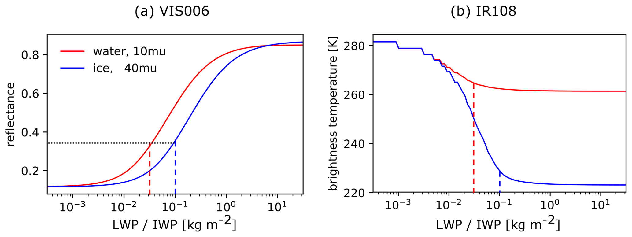
Figure 2Water and ice cloud signals with different effective particle radii from 0.6 µm SEVIRI solar reflectance (VIS006) (a) and 10.8 µm SEVIRI brightness temperature (IR108) (b), computed using DISORT. Dashed lines indicate saturation in IR108 for water (red) and ice (blue) clouds. The albedo was set to 0.1, the solar zenith angle was set to 30∘, the satellite zenith angle was set to 60∘ and the scattering angle was set to 135∘.
Both solar reflectance and infrared brightness temperature strongly depend on the LWP and IWP, although in different ranges: VIS006 is most sensitive to LWP/IWP values in the [10−2, 100] kg m−2 range, whereas the sensitivity of IR108 is limited to thinner clouds with values in the [10−2, 10−1] kg m−2 range due to fast saturation of the signal by the absorption of photons. Figure 2b implies that only cloud-top height and its corresponding temperature determines the observed BT for a single-layer water cloud with LWP > 0.03 kg m−2 or a single-layer ice cloud with IWP > 0.1 kg m−2. Hence, the IR signal can provide the cloud-top temperature but does not allow for retrieval of the LWP/IWP. In contrast, the solar reflectance is only 0.35 at these threshold values and can still provide information on the water/ice content up to LWP/IWP values of about 1 kg m−2. These different and complementary sensitivities show that model evaluation with solar and thermal channels has the potential to provide more information on the nature of the systematic errors and to possibly identify specific shortcomings that would not be visible by only examining a single channel.
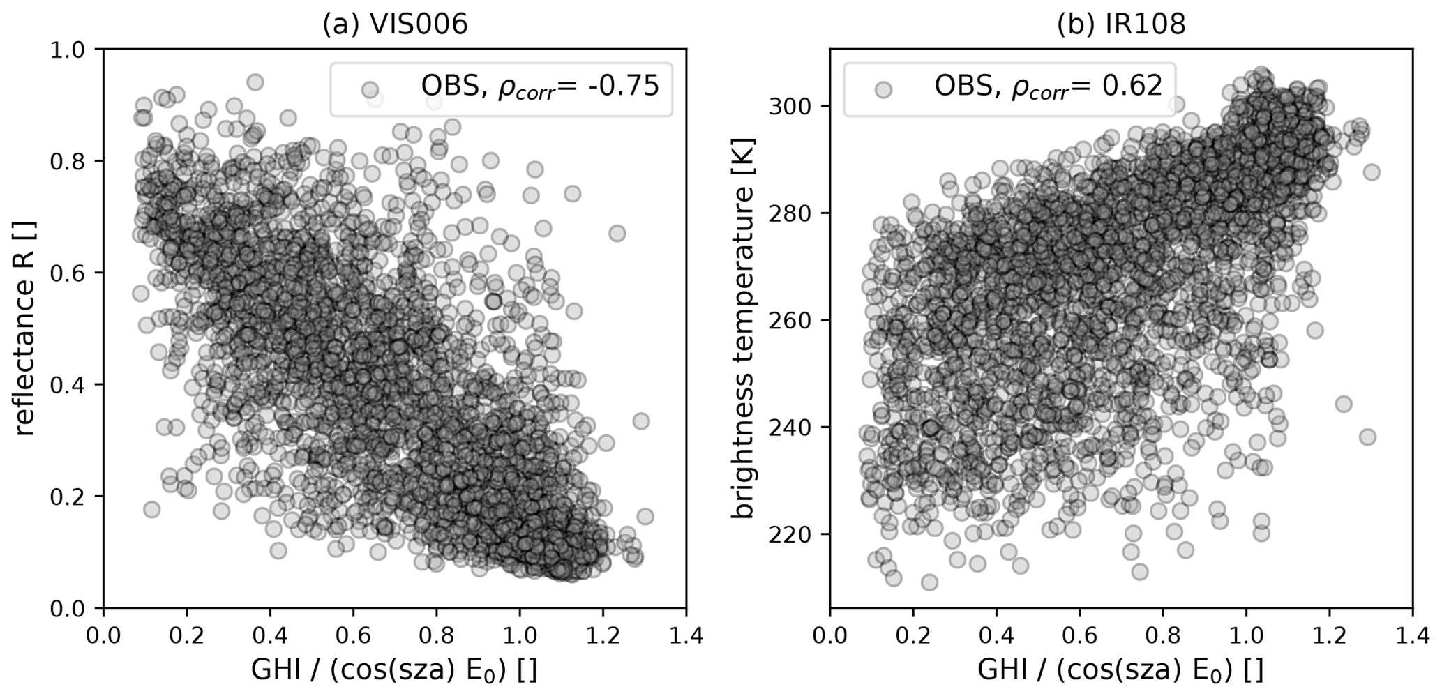
Figure 3The 0.6 µm SEVIRI solar reflectance (VIS006) (a) and 10.8 µm SEVIRI brightness temperature (IR108) (b) against the fraction of incoming global horizontal irradiance () at 12:00 UTC. Here, E0 (solar constant) is assumed to be 1367 W m−2, and the number of co-located observations at pyranometer stations is 3365.
An interesting consequence of these different sensitivities is that one would expect visible reflectance to provide more information on the transmittance of solar radiation to the surface than infrared radiances, as this process depends strongly on the water content of the clouds. Therefore, visible reflectances should be more strongly correlated with the incoming radiation at the surface than infrared brightness temperatures. This is confirmed by Fig. 3, which displays the correlations between the observed signals of the two satellite channels and normalised hourly averages of the global horizontal irradiance (GHI) measured at 122 DWD pyranometer stations (Fig. 1). There is indeed a strong negative correlation between the visible reflectance and the surface radiation, with a correlation coefficient (Fig. 3a). The anticorrelation is strong but not perfect due to the following reasons: (1) the instantaneous solar reflectance is compared to the time-averaged quantity GHI, (2) reflectance is averaged over pixels but GHI is a point measurement, and (3) 3D radiative transfer effects modify reflectance and GHI in different ways. For constant water content, surface radiation should not be strongly correlated with the cloud-top height or temperature. However, as many high clouds are caused by convection and these clouds contain large amounts of water, there is also some correlation between brightness temperature and surface radiation (Fig. 3b), but it is weaker (ρobs=0.62) than for the visible reflectances. These results indicate that by reducing the error of synthetic satellite images, in particular for visible satellite channels, it should be possible to improve radiation forecasts.
2.3 Satellite forward operators
To compute model equivalents for visible satellite images from the ICON model state, we employ the VISible satellite image Forward OPerator (VISOP) that uses the MFASIS 1D radiative transfer (RT) method (Scheck et al., 2016). MFASIS is based on a compressed lookup table (LUT), computed using the DISORT solver, where the aerosol optical depth (AOD) is assumed to be zero. However, it is possible to consider aerosols or different kinds of ice habits for the computation of the MFASIS LUT (results in Sect. 4.2). VISOP takes the slant satellite viewing angle into account (tilted independent column approximation; Wapler and Mayer, 2008) and accounts for the most important 3D RT effect by using the cloud-top inclination correction (CTI) described in Scheck et al. (2018). The surface albedo values required as input for MFASIS are taken from the RTTOV BRDF atlas (Vidot et al., 2018).
As we aim to achieve consistent assumptions in both the operator and the NWP model, we decided to use effective radii from the microphysics for water clouds directly. This is based on the consideration that radiative transfer, micro-physics and possibly operators should deal with the same optical properties.
However, some adjustments are required for the ice clouds, as will be motivated in the following. The micro-physics scheme in the simulation predicts six hydrometeor categories: cloud water, cloud ice and precipitating liquid water, snow, hail, and graupel. Rain droplets, hail and graupel particles are assumed to be much larger than cloud droplets and cloud ice particles in the model. Therefore, for the same mass, they are also much less effective at scattering radiation and are, thus, neglected in the forward operators. However, the distinction between snow and cloud ice particles in the model is rather artificial. Model snow particles can be small enough to cause non-negligible scattering effects (see discussion in Hogan et al., 2001). Hence, as a (first) approximation, we construct a frozen phase whose total mass, , is the sum of the diagnosed ice water content (grid- and subgrid-scale) and snow content (only grid scale available) and whose “effective effective radius”,
is defined using the simulated effective radii of cloud ice ri,eff and snow rs,eff. The effective radii for ice and snow are calculated under the assumption that both hydrometeors behave as randomly oriented needles, and using the mass–size relationships, size distributions and number concentrations from the microphysics (for details, see Fu et al., 1997, and Muskatel et al., 2021). This approximation assumes that the optical thickness of the frozen phase is equal to the sum of the optical thicknesses of the ice and snow phases, similar to the work of Senf and Deneke (2017). The approximation becomes exact in the case of wavelengths much smaller than the hydrometeors' size (optical limit); therefore, it is quite appropriate for visible channels.
In general, we use the diagnosed cloud water content and ice content including subgrid contributions as input for VISOP. If no subgrid-scale cloud is diagnosed in a particular grid box, , where x could be either water or ice. We assume no differences in the microphysical and optical properties of grid and subgrid clouds, so that the effective radius calculation is the same for both cases.
An accurate calibration is a prerequisite for using satellite observations, but unfortunately the calibration of SEVIRI VIS006 is uncertain. Meirink et al. (2013), for example, found a bias of −8 % for VIS006 during the period from 2004 to 2008 by comparing MSG SEVIRI and MODIS (Moderate Resolution Imaging Spectroradiometer) Aqua observations. For our purpose, we use the approach to find a suitable bias correction by minimising the average histogram difference between the observed and simulated solar reflectance distribution. Through this, we found a deviation of −13 % between observations and our reference simulation, which can be partly contributed to a calibration offset (observations too dark) and a model bias.
To derive SEVIRI infrared brightness temperature from the model state, we use the efficient methods implemented in the RTTOV 12.1 package (Saunders et al., 2018), which is used by many weather services.
For the evaluation, we applied both operators at the full model resolution and interpolated solar reflectances and the brightness temperature to the observation space afterwards to avoid additional representativeness errors (Marseille and Stoffelen, 2017).
2.4 Evaluation metrics
A combination of metrics is applied to evaluate synthetic satellite imagery at 12:00 UTC with observations. The evaluation domain (red rectangle in Fig. 1) is smaller than the ICON-D2 domain to exclude nesting effects at the domain boundaries and signals from snow-covered surfaces in the Alps that exhibit reflectances similar to clouds. We show the VIS006 and IR108 probability density functions of our simulations and observations P(R). The number of bins N of the PDFs is 50, with and K. From that, we define the cloudiness (C) as the fraction of pixels in which the solar reflectance is higher than a threshold value Rc of 0.2. This value is an upper limit for the clear-sky reflectance in the considered evaluation domain (see discussion in Scheck et al., 2018). Violin plots are used to visualise the daily bin-by-bin deviation of the PDF (deviation computed for each day d and bin n) from the reference run and model/operator sensitivity experiments: . This allows for a consistent comparison of VISOP and model uncertainty by examining the median deviation (the mean is always zero), the interquartile range (difference between 75th and 25th percentile) as a measure of variability and the range as the extent of deviations. We further analyse clouds by constructing contoured 2D PDF plots of brightness temperature and solar reflectance, comparable to the ISCCP approach (Rossow and Schiffer, 1991) or to contoured frequency by altitude diagrams (CFADs; Yuter and Houze, 1995) of radar observations. We use the US Standard Atmosphere 1962 (Sissenwine et al., 1962) to classify brightness temperatures into three cloud categories (low, middle and high clouds) as defined in the International Cloud Atlas (Cohn, 2017). In the US Standard Atmosphere, the surface temperature is 288 K and the (wet) temperature lapse rate is 0.65 K m, leading to temperature ranges of T>275 K for the surface and low clouds, 275 K ≤ T ≤ 243 K for middle clouds, and T<243 K for high clouds.
2.5 Synoptic overview and cloudiness
A 30 d period from 26 May to 24 June 2016 is analysed, which is dominated by strong summertime convection in Germany. In the beginning, large parts of Europe were affected by high-impact weather events over almost 2 weeks. Atmospheric blocking and the interaction of low thermal stability and weak mid-tropospheric winds were the ingredients for this exceptional sequence of thunderstorms and related flash floods (Piper et al., 2016). Many authors have discussed these 2 weeks (see e.g. Necker et al., 2020; Bachmann et al., 2020; Keil et al., 2019; Necker et al., 2018; Zeng et al., 2018). In the subsequent weeks (10–24 June), the wind direction changed to a south-westerly flow, advecting warm and humid air masses from the Atlantic and the Mediterranean to Germany and supporting cloud formation (Fig. 4). In general, the simulated cloudiness (defined in Sect. 2.4) is predominantly overestimated, leading to a mean observed and simulated cloudiness for the period of 0.73 and 0.76 respectively. This convective period with high cloud cover at different levels is well-suited to examine cloud statistics and its sensitivity to cloud-related parameterisations.
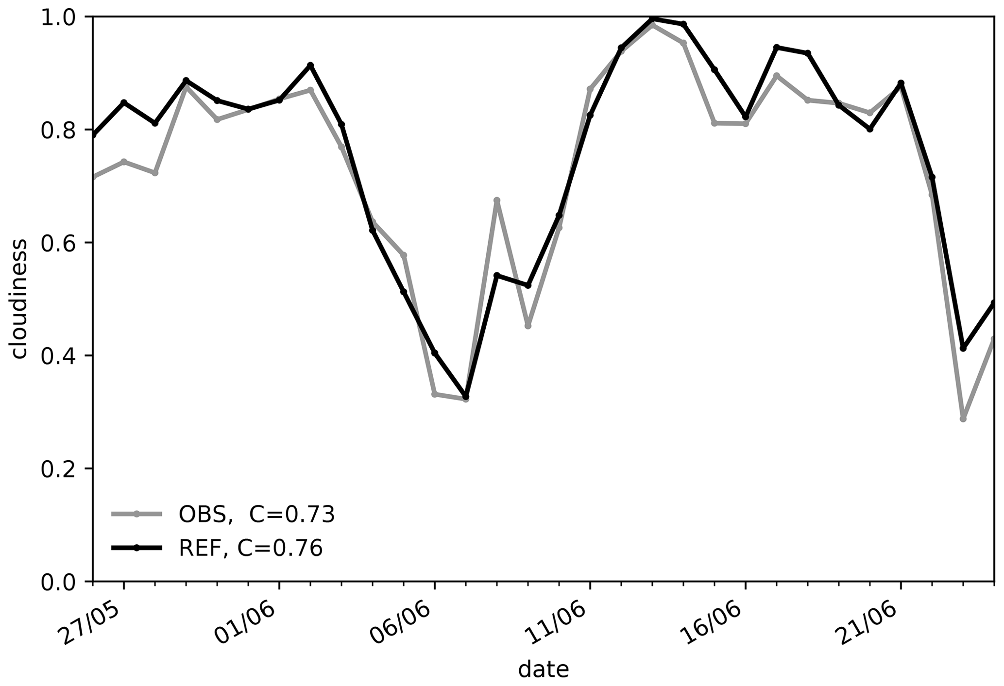
Figure 4Time series of observed and simulated cloudiness at 12:00 UTC during the period from 26 May to 24 June 2016. The cloudiness is defined as the fraction of pixels where 0.6 µm SEVIRI solar reflectance R>0.2.
3.1 Selected cases
In this section, we discuss 2 d of the period to illustrate the methodology for evaluating clouds using visible and infrared satellite channels. On the first day (29 May), deep convection and severe thunderstorms occurred, leading to a flash flood that caused severe damage in Braunsbach, a small town in the south-western part of Germany. The second day (2 June) was dominated by low-level clouds. According to Piper et al. (2016), warm, moist and unstable air masses characterised both days. However, large-scale ascent dominated on 29 May and subsidence dominated on 2 June. Figure 5 shows the VIS006 and IR108 satellite images as well as the corresponding distributions of solar reflectance and brightness temperatures on 29 May 2016. The VIS006 satellite image (Fig. 5a, c) shows the early stage of a cyclogenesis over Germany, characterised by a prominent vortex structure in both the observations and model simulation. However, the feature is shifted to the south-west in the simulation. The relatively high cloudiness of 88 % in the observations and 89 % in the simulation leads to a relatively uniform distribution of observed solar reflectances (Fig. 5e). Overall, the agreement between observed and simulated visible histograms is relatively good given that the model is forced towards the current weather only through the boundary conditions. The vortex structure of the cyclogenesis is also apparent in the IR108 observations (Fig. 5b), but the simulation shows clear systematic errors. In the simulation, the cloud pattern is dominated by relatively high ice clouds (Fig. 5d), which are less frequent in the observations. The histogram confirms this picture: the signal of high clouds is overestimated in the simulations, whereas the signal of medium clouds is underestimated by 40 %.
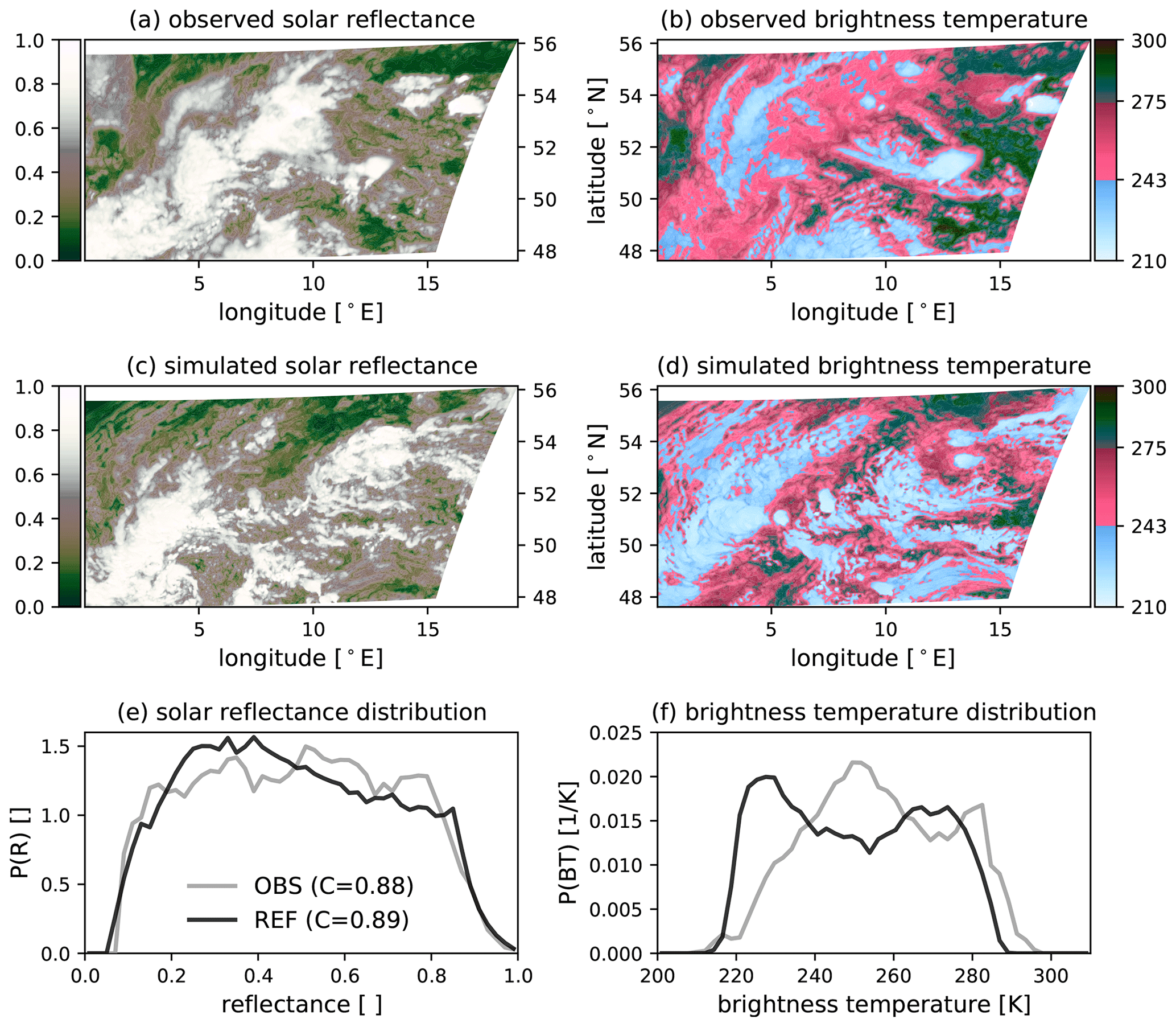
Figure 5The (regional) distribution of 0.6 µm SEVIRI solar reflectance (a, c, e) and 10.8 µm SEVIRI brightness temperature (b, d, f) as well as their corresponding distribution for 29 May at 12:00 UTC. The numbers in the legend of panel (e) indicate the cloudiness, i.e. the fraction of pixels exceeding a reflectance of 0.2 (EUMETSAT).
On 2 June 2016, boundary layer clouds dominated in both the observations and simulation (Fig. 6b, d). Additionally, superimposed ice clouds are observed in some regions. The simulated IR108 distribution fits the observed one relatively well on this day (Fig. 6f). In the visible satellite image (Fig. 6a, c), a high cloudiness is apparent, with 87 % in the observations and 91 % in the simulation. In contrast to 29 May, however, the distribution (Fig. 6e) reveals an overestimation of medium thick clouds as well as an underestimation of thick clouds (R>0.6).
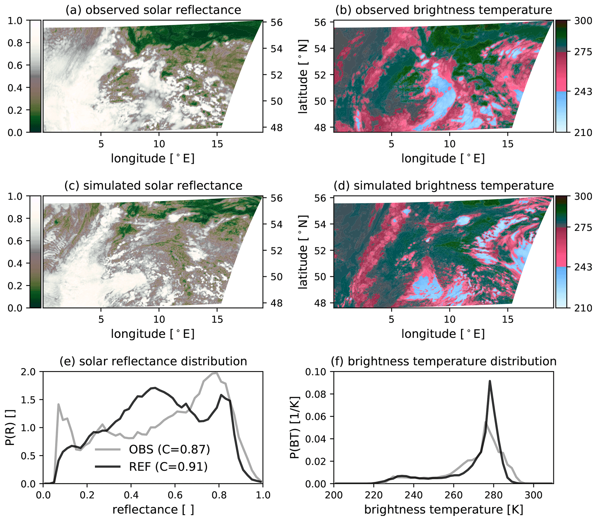
Figure 6The (regional) distribution of 0.6 µm SEVIRI solar reflectance (a, c, e) and 10.8 µm SEVIRI brightness temperature (b, d, f) as well as their corresponding distribution for 2 June 2016 at 12:00 UTC. The numbers in the legend of panel (e) indicate the cloudiness, i.e. the fraction of pixels exceeding a reflectance of 0.2 (EUMETSAT).
The examples discussed above show that the examination of a single channel (VIS or IR) can lead to opposite conclusions with respect to forecast quality. The agreement of the histograms for 29 May is good in the visible range but not in the IR; the opposite is observed for the 2 June. This shows that both channels provide complementary information. In the following, we show that further information can be obtained by using the combined information of both channels in 2D PDF plots of brightness temperature and reflectance. We have already discussed how the IR histogram shows an overestimation of high clouds on the 29 May. The combined histograms (Fig. 7a, c) provide the additional information that this overestimation of clouds mostly happens for thick clouds (R>0.6). This indicates that the model produced overly strong deep convection. On 2 June, where lower clouds dominated the scene, the observations and simulations agree on the vertical location of the shallow cumulus clouds (Fig. 7b, d). However, solar reflectances are primarily distributed around 0.7 in the observations and around 0.5 in the simulation. Compared with the 1D reflectance histogram, the 2D PDF provides the additional information that the systematic reflectance errors are related to low clouds. These 2 d with predominantly deep convective clouds (29 May) and low clouds (2 June) are for different cloud types and formation processes. Thus, their analysis illustrates the benefit of combining a visible and an infrared channel.

Figure 7Combined 0.6 µm SEVIRI solar reflectance (VIS006) and 10.8 µm SEVIRI brightness temperature (IR108) PDF of observations (a, b) and simulations (c, d) on 29 May (a, c) and 2 June 2016 (b, d) at 12:00 UTC.
3.2 VIS006 and IR108 statistics for the full period
The analysis of individual cases presented above illustrates certain characteristics, but longer periods are required to identify systematic model deficiencies. To address this, we now present results for the 30 d period. The observed mean VIS006 solar reflectance distribution at 12:00 UTC reveals a clear-sky peak at low reflectance values (), a nearly uniform distribution for higher reflectances () and a sharp decrease for reflectances higher than 0.8 (Fig. 8a). The distribution of the reference simulation overall looks similar, but it shows some deviations from the flat plateau seen for the observations, with a surplus of clouds around a reflectance of 0.5. Figure 8b presents a histogram of the 30 d mean IR108-BT at 12:00 UTC. There are generally too many clouds with low brightness temperatures (BT < 240 K). This, along with an underestimation of mid-level clouds in our ICON simulations, is a well-known issue that has been found for many global circulation or weather prediction models using forward operators or retrievals for evaluation (e.g. Illingworth et al., 2007; Pfeifer et al., 2010; Böhme et al., 2011; Franklin et al., 2013; Keller et al., 2016). Zhang et al. (2005) discussed possible reasons for the lack of mid-level clouds and concluded that physical deficiencies in the model might introduce these systematic deviations. The distribution further reveals a clear-sky bias, where the model underpredicts high BT values.
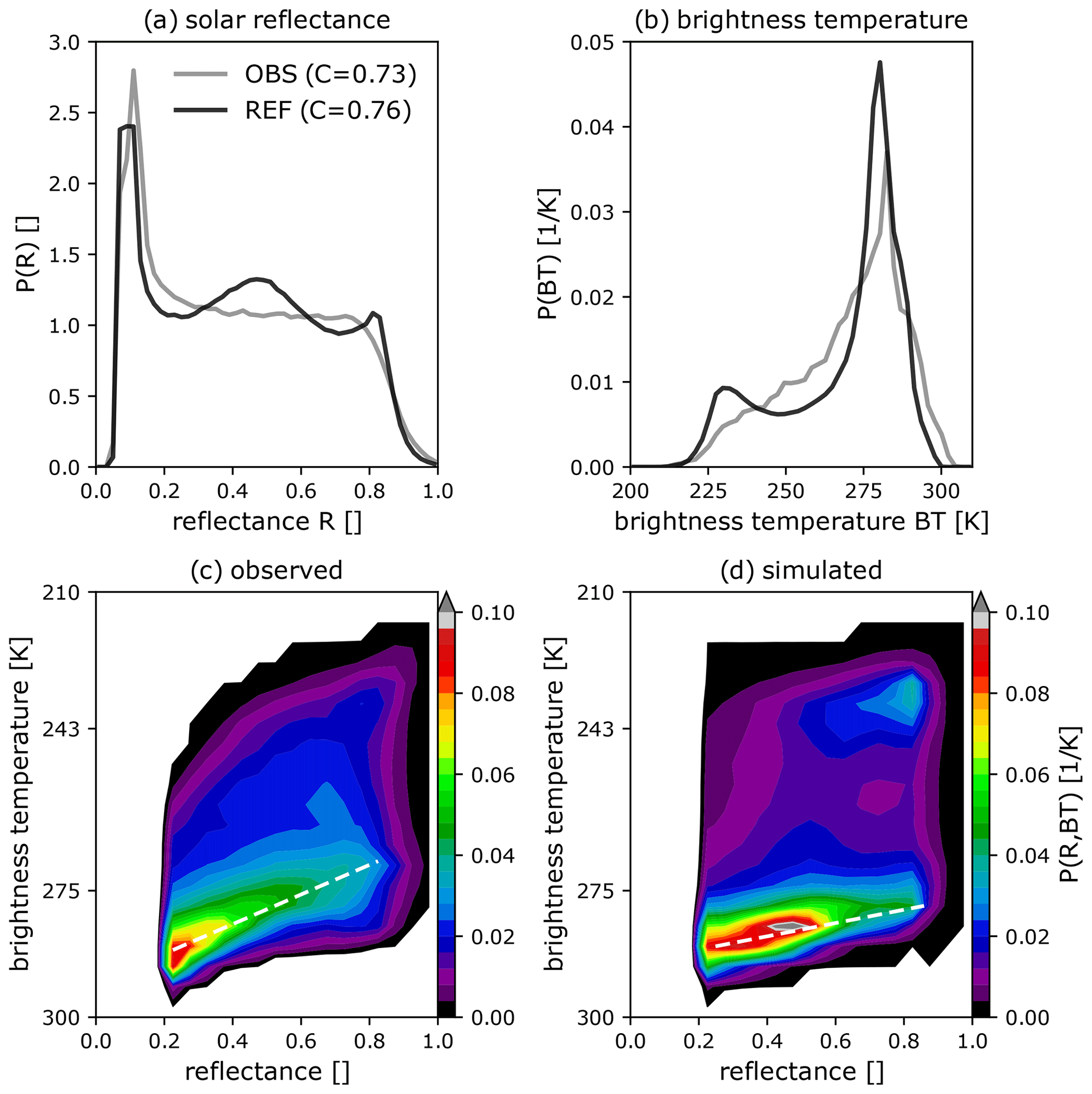
Figure 8Individual PDFs for 0.6 µm SEVIRI solar reflectance (VIS006) (a), 10.8 µm SEVIRI brightness temperature (IR108) (b) and combined VIS006–IR108 PDF (c, d) of observations (c) and simulations (d) at 12:00 UTC for the full test period. The numbers in the legend of panel (a) indicate the cloudiness, i.e. the fraction of pixels exceeding a reflectance of 0.2.
In general, the statistics for the full period, as shown by the 2D PDFs in Fig. 8c and d, indicates that the model and observation distributions have similar structures. Noticeable differences in the distribution occur in boundary layer clouds. The increase in solar reflectance with decreasing brightness temperature (increasing height) is noticeably steeper in the observations (indicated by dashed white lines in the plots). This means that thick boundary layer clouds consistently reach higher levels in the observations and suggests that shallow convection is too weak in the model. The 2D PDFs further indicate that the surplus of clouds around a reflectance of 0.5 in the model is related to boundary layer clouds, revealing a deficiency in the model representation of liquid water clouds. In addition, the simulation does not produce enough mid-level clouds at all solar reflectances. Finally, a secondary maximum at low BTs and high solar reflectance (R≈0.8) is apparent in the simulations but not in the observations. This maximum mainly corresponds to deep convective and precipitating clouds, which are either too active or produce too much ice, similar to 29 May. High-level clouds (cirrus as well as iced cloud tops) and low-level clouds are generally overestimated.
The combined histograms clearly show important shortcomings in shallow and deep convection. Thus, combined histograms can provide additional information on the nature of the systematic errors evident in the 1D histograms as well as very valuable information for model development, showing which model configuration produces more realistic clouds.
4.1 Contributions of different clouds to the reflectance distribution
To better understand the sensitivity of the synthetic visible satellite images to changes in operator settings and model modifications, it is helpful to determine the contribution of different hydrometeor types and subgrid-scale clouds to the reflectance histogram of the reference run (Fig. 8a). Figure 9 shows the observed and simulated VIS006 solar reflectance distribution (OBS and REF are the same as in Fig. 8a), the distribution that results from taking only grid-scale clouds into account (REF-grid) and several distributions obtained by using only certain types or combinations of hydrometeors. By comparing the contribution of a certain cloud type, e.g. REF − REF-grid for the subgrid clouds, to the deviation of REF from OBS, one can infer if tuning (i.e. slightly changing) parameters related to this cloud type in the model or the operator could be helpful to reduce REF − OBS. The shapes of the curves can provide further information regarding this question. Cloudiness values C are provided for each case in Fig. 9 to better quantify the relative importance of different cloud contributions.
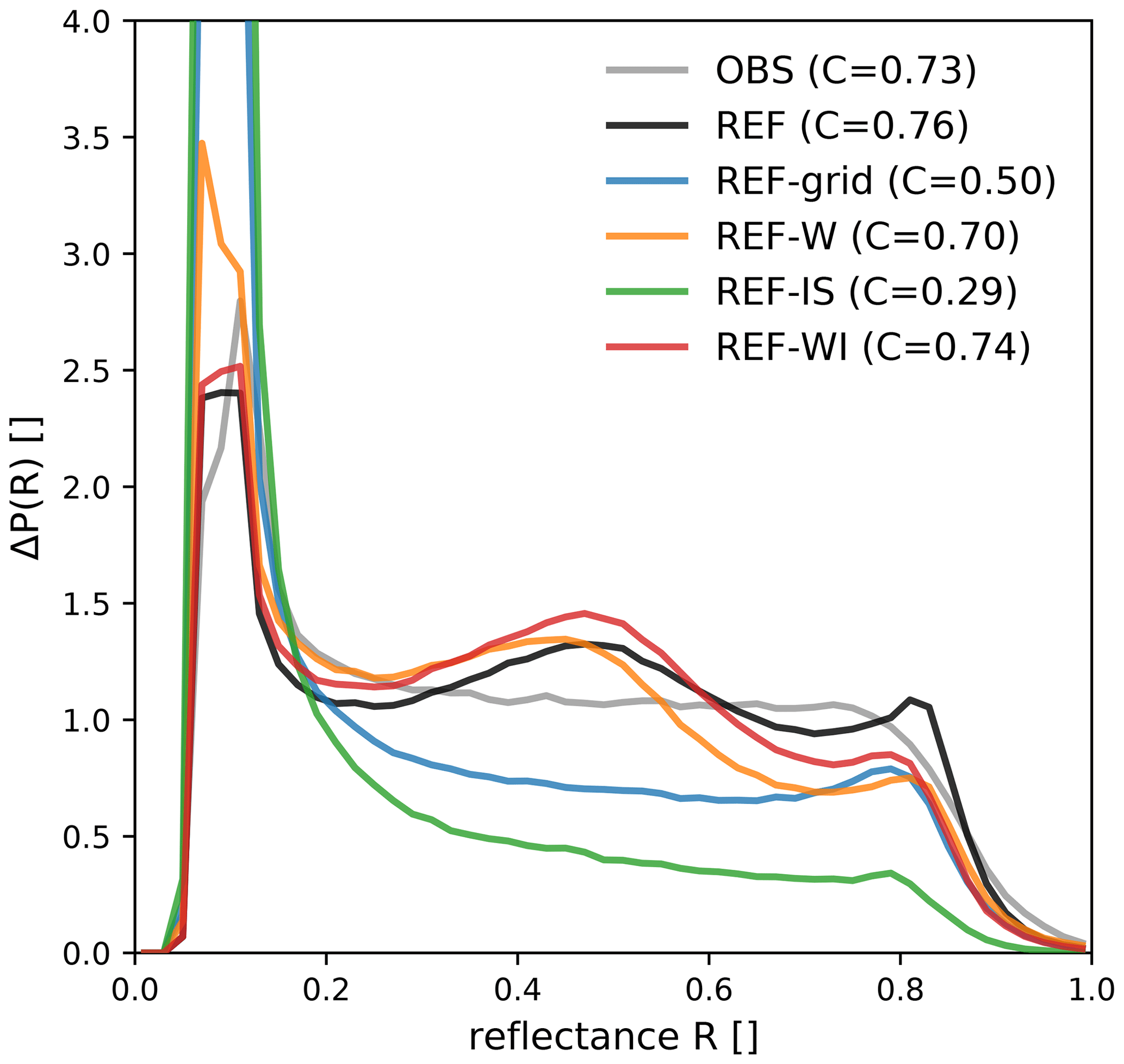
Figure 9The 0.6 µm SEVIRI solar reflectance histograms for the test period computed for the observations (OBS) and the reference experiment (REF). The additional distributions were computed using only the grid-scale clouds (REF-grid), only the water clouds (REF-W) and only the ice clouds (REF-IS) of the reference experiment respectively. For the red line (REF-WI), water and ice clouds are taken into account, and only the snow contribution to the ice clouds is omitted. The numbers in the legend indicate the cloudiness, i.e. the fraction of pixels exceeding a reflectance of 0.2.
Grid-scale clouds only lead to a distribution with a nearly flat plateau between reflectances of 0.3 and 0.7, a feature that is also found in the distribution of the observed reflectances. However, the fraction of cloud pixels would decrease from C=0.76 to 0.5 if only grid-scale clouds were present. Adding subgrid clouds results in much better agreement with the observed value of C=0.73. It is, thus, essential to take these additional subgrid clouds into account. However, the imperfect parameterisation of subgrid clouds also contributes to deviations in the shape of the distribution: while the distributions of the observations and the grid-scale-clouds-only simulation exhibit a relatively flat plateau, the addition of subgrid clouds leads to a histogram curve with a pronounced maximum at 0.5 and a minimum at 0.7.
When only water clouds are used as input to the operator (REF-W), the cloudiness falls off from C=0.76 to C=0.70. Primarily, reflectances larger than 0.5 become slightly less frequent. In contrast, taking only ice clouds (including snow) into account (REF-IS) has a more substantial impact on the histogram and results in a much smaller cloudiness of C=0.29. Thus, water clouds play a much more substantial role in the reflectance distribution than ice clouds. This result is not surprising, as the ice water path is much smaller than the liquid water path, and larger ice particles are also less effective at scattering light than smaller water droplets (Fig. 2a).
In both the water-only and the ice-only cases, the corresponding subgrid clouds are included. The water-only curve (REF-W) shows the same deviation from the plateau-like shape of the observed distribution as the curve computed for all clouds (REF), but the ice-only curve (REF-IS) does not. Thus, it seems that the subgrid water cloud parameterisation needs to be improved to get better agreement in the histogram shapes. Finally, ignoring the simulated snow content (REF-WI) has a small but detrimental effect. This emphasises the need to include snow in the computation of the RT input variables, as discussed in Sect. 2.3.
4.2 Estimated uncertainty of VISOP
Forward operators use fast, approximate RT methods and rely on the limited information that is available from the NWP model. Due to missing 3D RT effects and missing information (e.g. on unresolved cloud properties), their output is to some extent uncertain. While forward operators for thermal infrared channels have been available for some time and their uncertainties have been investigated in several studies (e.g. Senf and Deneke, 2017; Saunders et al., 2017, 2018), no such information is available for visible channels. In the following, the uncertainty related to what we regard as the most critical error sources will be estimated by varying the corresponding operator settings.
The potential sources of uncertainty to be investigated are related to missing 3D RT effects, unknown or inconsistent overlap statistics of subgrid-scale clouds, the spatial and temporal variation of aerosols, and the shape of cloud ice particles. To estimate the upper limits of the uncertainty in the reflectance distribution related to these sources, we repeated the computation of visible reflectances applying VISOP to the reference simulation with deactivated cloud-top inclination (CTI) parameterisation, random instead of random-maximum subgrid cloud overlap, and aerosols or a different kind of ice habit included in the MFASIS LUT. The deviations in the reflectance distribution for the reference run caused by changing these operator settings are shown in Fig. 10.
The subgrid cloud overlap assumptions would not be a source of operator uncertainty if the assumptions in the NWP model and the operator were entirely consistent. However, the near-operational version of ICON employed to perform the model runs for this study uses inconsistent overlap assumptions in the infrared and visible part of the spectrum. This inconsistency will likely be corrected in future versions, but at the moment, it means that the operator cannot be entirely consistent with the model. The deviation in the reflectance distribution caused by changing the assumption from maximum-random to random in the operator (orange line in Fig. 10) can be regarded as an upper limit for the impact. Changing the assumption shifts the peak around R=0.5 (which is related to subgrid clouds, as discussed in Sect. 4.1) to higher reflectances but does not have much influence on reflectances larger than 0.7.
Missing or imperfectly modelled 3D RT effects are likely the source of uncertainty that is most difficult to quantify. According to Scheck et al. (2018), the most important 3D effect is related to the inclination of the cloud-top surface, which influences the observed reflectance. The parts of the cloud-top surface tilted towards the Sun appear brighter, and those tilted away from the Sun appear darker. The cloud-top inclination correction (CTI; see Scheck et al., 2018) accounting for this effect has been shown to reduce the error with respect to full 3D RT calculations and is included in the reference run. The main effect of the CTI on the reflectance histogram is to reduce the slope at the high-reflectance end of the distribution and to bring it in better agreement with observations. Switching off the CTI leads to an overly steep decline of the distribution at high reflectances, which is visible as a double-peak structure at R>0.8 in Fig. 10. Other 3D RT effects like cloud shadows may also play a role, in particular for larger zenith angles. However, by focusing on observations near local noon, their influence should be minimised.
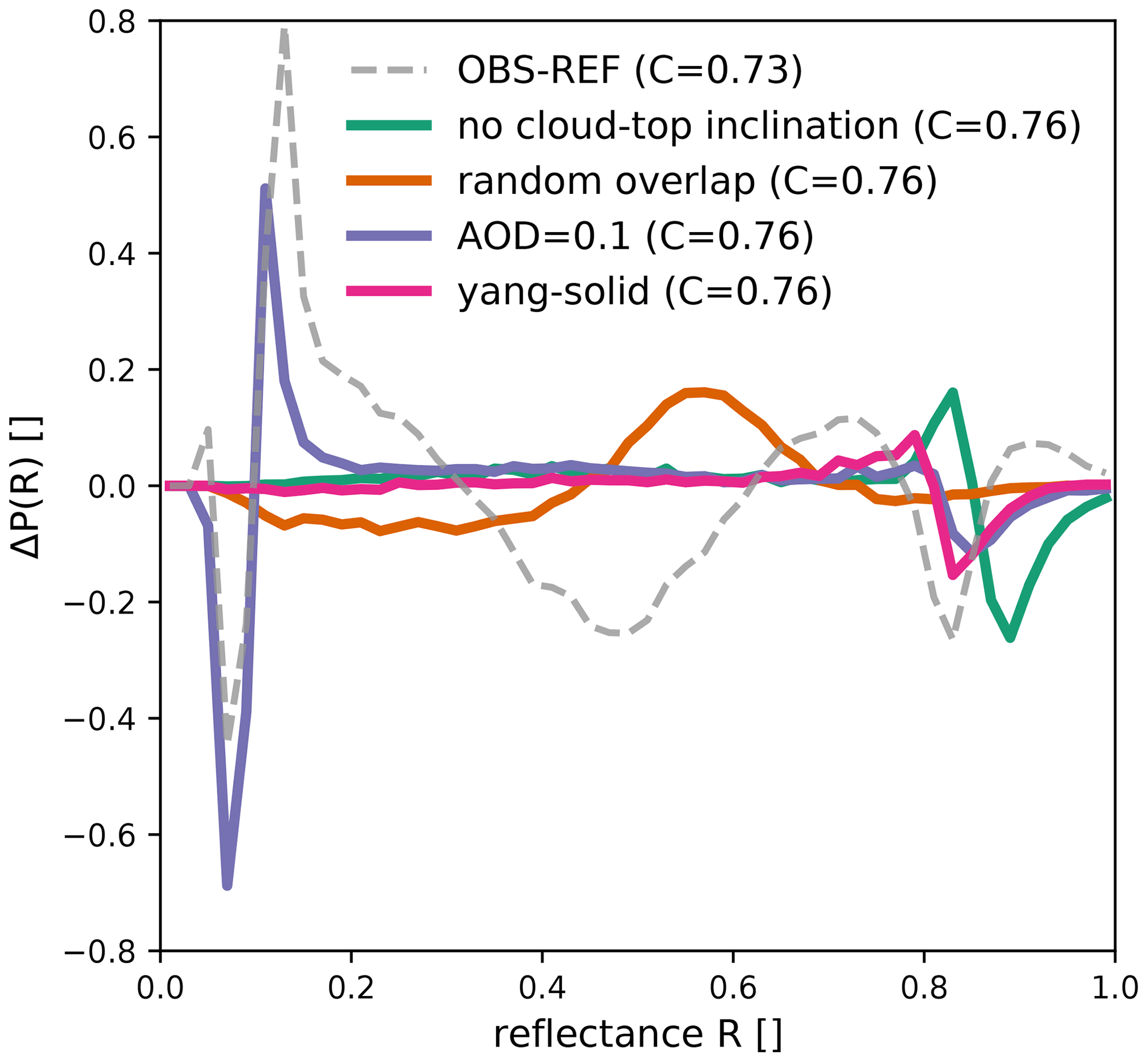
Figure 10Differences between the 0.6 µm SEVIRI solar reflectance PDFs obtained for the reference run with modified operator settings and standard settings. The modified settings are switching off the cloud-top inclination, using random instead of maximum-random subgrid cloud overlap, including aerosols with an optical depth of 0.1 and changing the cloud ice particle habit to solid columns. For comparison, the difference between the observations and the reference run histogram is also shown (dashed curve).
According to retrievals based on measurements at AERONET (AErosol RObotic NETwork) stations (see Giles et al., 2019) in Germany, the mean AOD in June 2016 was in the range of 0.06 to 0.12 at a wavelength of 675 nm, which is similar to the wavelength of the visible channel considered here. To estimate the impact of these aerosols on the reflectance histogram, an MFASIS LUT was computed that includes aerosols (the “continental clean” aerosol mixture available in libRadtran; see Emde et al., 2016) with an optical depth of 0.1. Including aerosols in the MFASIS LUT (i.e. taking direct aerosols effect into account) influences the reflectance histogram in two ways. Under clear-sky conditions, the reflectance increases because aerosols scatter photons to the satellite, whereas under cloudy conditions, aerosols scatter photons out of their path towards the satellite. Thus, in the presence of aerosols, the high-reflectance end of the distribution is shifted towards lower reflectances, and the low-reflectance end is shifted towards higher reflectances. Shifting the pronounced ground peak in the distribution causes a double-peak structure at low reflectances in Fig. 10, whereas shifting the flat high-reflectance end only causes a single negative peak. In general, the error introduced by direct aerosol effects for events like (Saharan) dust outbreaks can be higher and could potentially lead to significant errors in solar reflectances. Thus, days affected by such events, which did not occur during our test period, should be excluded from model evaluation studies.
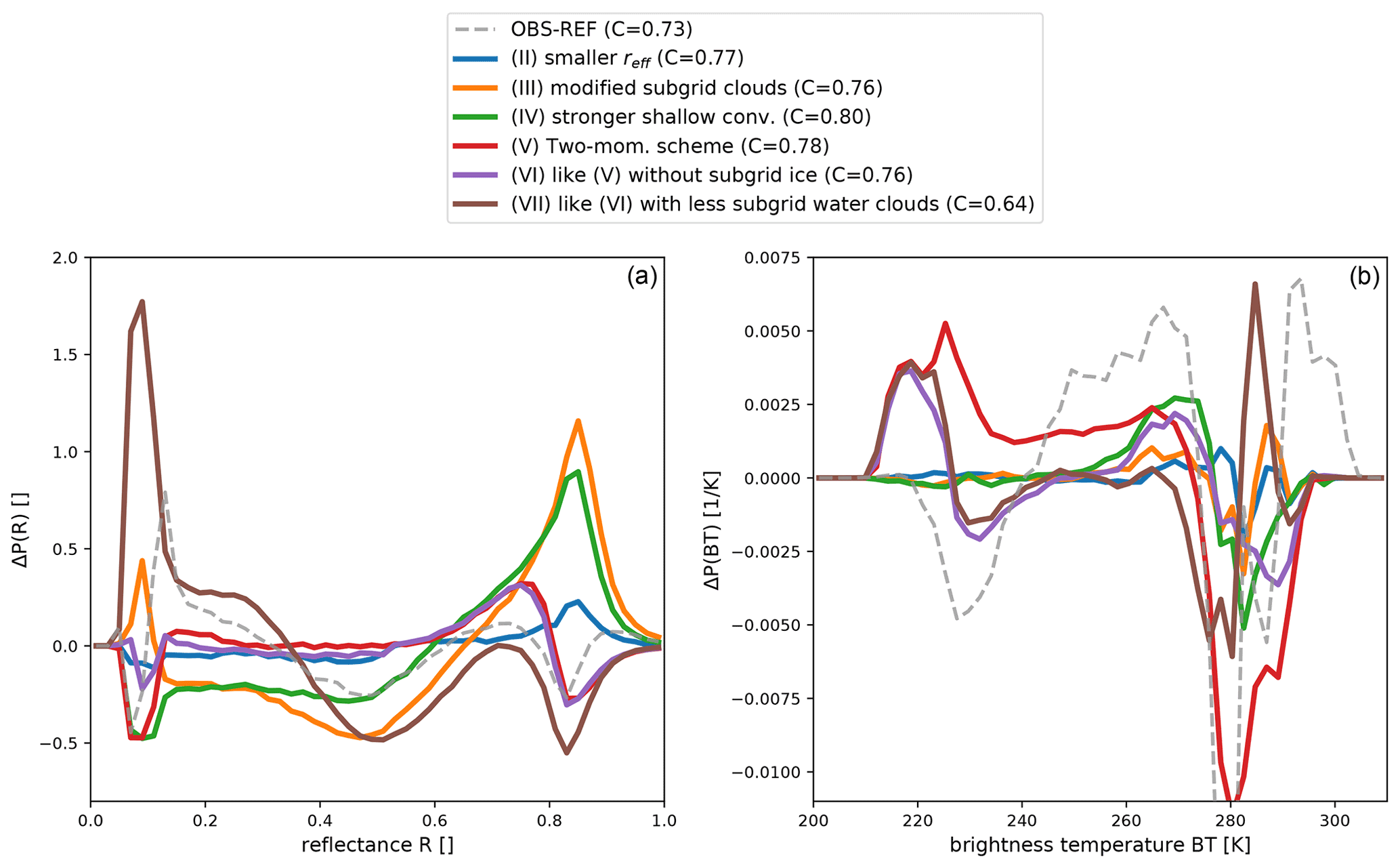
Figure 11Differences in the 0.6 µm SEVIRI solar reflectance (a) and 10.8 µm SEVIRI brightness temperature (b) PDFs between perturbed model simulations and the reference run. The perturbed model settings are (II) increased cloud droplet number concentration (smaller effective radius) due to increased updraught velocity at activation, (III) modified distribution of turbulent subgrid liquid clouds (less and thicker subgrid clouds), (IV) stronger shallow-convection parameterisation due to doubled thickness of the thickest unresolved cloud, (V) simulation with the two-moment scheme, (VI) is like (V) but without subgrid-ice clouds, and (VII) is like (VI) but with a reduced number of subgrid-scale liquid clouds. For comparison, the difference between the observations and the reference run histogram is also shown (dashed curve).
Finally, the shape of cloud ice particles is also an uncertain factor that influences the reflectances' distribution. Changing the shapes quite strongly from the baum_v36 general habit mixture (Baum et al., 2014) to solid columns (using the optical properties of Yang et al., 2005) basically only affects the highest reflectances, which are slightly reduced. Hence, the ice habit is not likely to cause large uncertainties in the reflectance distribution for our test period, which is characterised by a high low-level cloud cover and overlaying semi-transparent cirrus clouds. For periods with more and thicker ice clouds, the uncertainties could be higher.
4.3 Sensitivity to model settings
Figure 11 shows the deviations of the reflectance and BT distributions computed for model runs using modified settings (see Sect. 2.1) with respect to the reference run. In general, these deviations are of a similar magnitude to the systematic deviations between the observations and the model equivalents for the reference run discussed in Sect. 3 (see dashed curve in Fig. 11). In Sect. 3, we identified several reasons for systematic deviations between the simulations and observations: an underestimation of thick clouds (), an overly low boundary layer height, too many high clouds and an insufficient representation of low-level water clouds. As further analysed in Sect. 4.1, we found that the discrepancy in low-level clouds mainly arises from subgrid water clouds ().
Figure 11a shows the effect of model modifications on the reflectance distribution. The first modification (experiment II), reducing the effective radii by increasing the updraught velocity and, thus, also the number of cloud condensation nuclei, leads to more thick clouds with R>0.7 and less thin clouds with R<0.5. Changing the subgrid cloud parameters (experiment III) or reinforcing shallow convection (experiment IV) has a qualitatively similar but much stronger impact on the reflectance distribution. Pixels with dense clouds become more numerous, and the number of pixels with thin to medium clouds is reduced. These changes are larger than the deviations of the reference run (experiment I) from the observations (dashed line in Fig. 11a). In the case of modified shallow convection, the cloudiness increases from 0.76 to 0.8, which means that the deviation from the observed value of 0.73 is considerably larger.
Switching to the double-moment microphysics scheme (experiment V) mainly moves pixels with very high reflectances (R>0.8) to somewhat lower reflectance values between 0.6 and 0.8 and increases the cloudiness slightly. Thin to intermediate clouds () are only weakly affected. Still using the two-moment scheme but turning off subgrid-scale ice clouds (experiment VI) slightly decreases the cloudiness but basically leads to the same distribution as experiment V. Hence, ice subgrid-scale clouds cannot be responsible for the surplus of pixels with solar reflectances around R=0.5 that was attributed to subgrid clouds in Sect. 4.1. Finally, reducing the subgrid-scale water clouds (experiment VII) also leads to much larger changes, with negative peaks around R=0.5 and R=0.8 and positive values for R<0.35. These changes point in the right direction with respect to mitigating the deviations of the reference run (dashed line in Fig. 11a). However, the modification is too strong here, as cloudiness is dramatically underpredicted in this case (C=0.64). Compared with visible reflectances, the changes in the BT distribution introduced by modified model settings are more difficult to interpret because the signal depends on cloud optical depth as well as on cloud-top height. The modifications in experiments II and III only affect water clouds and, thus, only lead to changes at higher BTs. These changes are relatively small compared with those required to correct the deviations in the reference run (dashed line). Making shallow convection stronger (experiment IV) has a stronger impact and increases the number of pixels with BT values between 250 and 275 K at the expense of those with higher values. Switching to the double-moment scheme (experiment V) increases the number of middle to very high clouds for BT < 270 K and introduces a substantial reduction of the clear-sky and low-level cloud signal (BT around 280 K). These changes indicate that the two-moment scheme generates even more dense ice clouds than the one-moment scheme in the reference run, which already predicts too many of these clouds. These high clouds obscure lower clouds and the surface, which leads to less pixels with high BTs. Switching off subgrid ice clouds in the two-moment simulation (experiment VI) reveals that the peak around BT = 220 K is related to grid-scale clouds in the double-moment scheme, and the distribution of middle clouds is more like the single-moment simulation. Additionally modifying the subgrid liquid water clouds (experiment VII) again mainly affects the clear-sky and lower-level cloud signal.
Comparing the changes in the reflectance and BT distribution that were introduced by modified model settings within their estimated uncertainty leads to the following interpretation: the reflectance distribution is mainly affected by changes to water clouds and is only weakly influenced by changes to ice clouds. In contrast, the BT distribution is most strongly affected by changes in the ice clouds, but modified water clouds also have some influence on higher BTs. The distinct changes in the distributions caused by the individual model modifications allow one to assess which modification could be useful to mitigate deviations from the observed distributions.
The results shown in Fig. 11a indicate that a modified version of experiment VII with weaker modifications or a combination of II, III and IV could be able to achieve the corrections required for the reference run, i.e. to reproduce the dashed line (OBS-REF). In both cases the subgrid water clouds play an important role. Therefore, to correct systematic errors in the reflectance distributions, it seems particularly important to tune or advance the subgrid cloud scheme. While the reflectance distribution is not sensitive to changes in subgrid ice clouds, these are clearly important for the BT distribution (compare experiments V and VI in Fig. 11a and b). The combined information from the two parts of the spectrum can, thus, provide guidance on optimising the subgrid cloud scheme.
In contrast to visible reflectances, there is no obvious way to scale or combine the model modifications in order to eliminate the errors of the reference run in the IR108 channel, i.e. to reproduce the dashed line in Fig. 11b. Additional or different model modifications appear to be required for this purpose, but the results presented here already indicate that particular modifications leading to less grid-scale ice clouds are required.
It should be noted that the results presented in this study were obtained for a summer period, in which the reflectance was clearly dominated by water clouds. For situations in which ice clouds play a more important role, the visible channel should still provide better information on the total (liquid and frozen) water content than the infrared channel. However, it could be more problematic to attribute systematic deviations in the reflectance histograms to water or ice clouds, and the error related to assumptions on the ice habit may be larger. Also using the 1.6 µm channel, which allows for distinguishing water from ice clouds, may be helpful in these cases.

Figure 12Distributions of daily bin-by-bin differences from the reference run in the 0.6 µm SEVIRI solar reflectance as a measure of uncertainty in the visible forward operator (a) and the model (b). The modified forward operator settings are switching off the cloud-top inclination (3D effects), using random instead of maximum-random subgrid cloud overlap (overlap), including aerosols with an optical depth of 0.1 (aerosols) and changing the cloud ice particle habit to solid columns (ice habits). The perturbed model settings are (II) increased cloud droplet number concentration (smaller effective radius) due to increased updraught velocity at activation, (III) modified distribution of turbulent subgrid liquid clouds (less and thicker subgrid clouds), (IV) stronger shallow-convection parameterisation due to doubled thickness of the thickest unresolved cloud, (V) simulation with the two-moment scheme, (VI) is like (V) but without subgrid-ice clouds, and (VII) is like (VI) but with a reduced number of subgrid-scale liquid clouds. The horizontal dashed lines indicates 25th, 50th (median) and 75th percentiles.
4.4 Sensitivity intercomparison for visible reflectances
The comparison of Figs. 10 and 11a already indicates a considerably larger effect of model modifications compared with that of operator uncertainties on the reflectance distribution for the full test period. To provide a clearer comparison of the impact of model modifications and operator uncertainties, we computed the individual changes on each day of the test period in all of the reflectance bins (see Sect. 2.4). The violin plots in Fig. 12 show these daily bin-by-bin deviations of the reflectance distribution caused by changes in the operator settings and model modifications. Figure 12 indicates that the changes due to model modifications are also much larger for individual days of the test period than those related to operator uncertainty. The median deviation and the interquartile range (difference between the 75th and 25th percentile) are about 1 order of magnitude larger for the model uncertainty. As already mentioned, aerosols will have a much stronger impact during situations such as dust events, but such events should not be included in test periods for the evaluation of model clouds.
In general, the operator uncertainties are thus a second-order effect compared with model modifications. Visible satellite images are, therefore, well-suited to detect and overcome model deficiencies and to provide guidance for model tuning. Still, some of the deviations in the model reflectance distribution could be related to operator deficiencies. An improved cloud-top inclination or changes in the cloud ice optical properties could mitigate some of the deviations at high reflectances, and using the correct aerosol optical depth can particularly improve the low-reflectance end of the distribution (see Fig. 10). However, for a broad range of reflectances, between 0.2 and 0.8, it is only the inconsistency in the overlap assumption that makes the operator results uncertain. As discussed above, this is actually only a temporary issue related to the current versions of the ICON model. As soon as the overlap assumptions in the model are consistent, the correct choice of the overlap assumption can be regarded as a model setting, and model evaluation using visible reflectances can provide information on suitable choices.
We investigated systematic differences between satellite observations and corresponding synthetic observations from the preoperational ICON-D2 model to better understand the representation of clouds and radiation in NWP models. For this purpose, a semi-free 30 d convection-permitting hindcast simulation was conducted that is only forced by low-resolution analysis boundary conditions for a highly convective period in May/June 2016. Furthermore, additional simulations with modified model settings were conducted to identify dominant error sources and identify potential approaches for improving the representation of clouds in ICON-D2.
In contrast to previous studies, we did not compare quantities retrieved from the satellite observations to the model state; instead, we performed the comparison in observation space using synthetic satellite images generated by forward operators. The fact that the errors in the synthetic images are easier to characterise than for retrievals is considered to be an advantage of this approach. As using visible satellite images generated by a fast forward operator in this approach is not yet well established for evaluation, we conducted a number of sensitivity experiments with modified operator settings to investigate the recently developed forward operator's uncertainty transforming from model to observations space. The comparison revealed that the operator uncertainty is roughly 1 order of magnitude smaller than the sensitivity of the results to modified model settings. This further emphasises the usefulness of solar channels for model evaluation and improvement.
The combination of observations in two spectral ranges provides significantly more and complementary information than the individual channels. While infrared observations provide information on cloud-top height, their signal quickly saturates in the presence of clouds. This means that infrared observations can only distinguish a small range of cloud water contents, and information on water clouds may be obscured by cirrus clouds above. In contrast, visible channels are less sensitive to ice clouds and can distinguish a much more extensive range in the cloud water path (liquid and solid). The combined use of visible and infrared observations also allowed us to identify specific model deficiencies (e.g. too many high cirrus clouds, overly weak shallow convection, deficiencies in the model representation of subgrid clouds, overly strong deep convection or excessive production of cloud ice). Several model sensitivity experiments targeted these deficiencies and point towards potential approaches for model improvement. However, solving these challenging issues will require additional studies given the number of interacting processes that contribute to the formation, modification and dissipation of clouds. Nevertheless, it is of utmost importance to advance the representation of clouds and radiation for the use of cloud-affected satellite observations in data assimilation, the prediction of PV power production and, last but not least, accurate climate simulations.
The relevant research data (observations and model equivalents) are publicly available at https://doi.org/10.5281/zenodo.4548922 (Geiss et al., 2021). The model simulation output will be archived at the Leibniz Supercomputing Centre (LRZ) for 10 years.
AL carried out the model simulations. SG applied the operator to model output, made most of the figures and analysed the data. LS provided satellite observations and made one of the figures. SG, LS, AL and MW contributed to the writing the paper, discussions and analysis of the figures.
The authors declare that they have no conflict of interest.
Publisher's note: Copernicus Publications remains neutral with regard to jurisdictional claims in published maps and institutional affiliations.
This study was carried out in the integrated project MetPVNet, which is financed by the Federal Ministry for Economic Affairs and Energy. The authors would like to thank the Hans Ertel Centre for Weather Research (Weissmann et al., 2014; Simmer et al., 2016) for supporting this work. This German research network of universities, research institutes and the German Weather Service is funded by the BMVI (Federal Ministry of Transport and Digital Infrastructure).
This research has been supported by the Bundesministerium für Wirtschaft und Energie (grant no. 0350009A).
This paper was edited by Philip Stier and reviewed by Matthew Igel and one anonymous referee.
Bachmann, K., Keil, C., Craig, G. C., Weissmann, M., and Welzbacher, C. A.: Predictability of deep convection in idealized and operational forecasts: Effects of radar data assimilation, orography, and synoptic weather regime, Mon. Weather Rev., 148, 63–81, 2020. a
Baldauf, M., Gebhardt, C., Theis, S., Ritter, B., and Schraf, C.: Beschreibung des operationellen Kürzestfristvorhersagemodells COSMO-D2 und COSMO-D2-EPS und seiner Ausgabe in die Datenbanken des DWD (2018), available at: https://www.dwd.de/SharedDocs/downloads/DE/modelldokumentationen/nwv/cosmo_d2/cosmo_d2_dbbeschr_version_1_0_201805.pdf?__blob=publicationFile&v=3 (last access: 14 August 2021) 2018. a
Baum, B. A., Yang, P., Heymsfield, A. J., Bansemer, A., Cole, B. H., Merrelli, A., Schmitt, C., and Wang, C.: Ice cloud single-scattering property models with the full phase matrix at wavelengths from 0.2 to 100 µm, J. Quant. Spectrosc. Ra., 146, 123–139, https://doi.org/10.1016/j.jqsrt.2014.02.029, 2014. a
Bechtold, P., Semane, N., Lopez, P., Chaboureau, J.-P., Beljaars, A., and Bormann, N.: Representing Equilibrium and Nonequilibrium Convection in Large-Scale Models, J. Atmos. Sci., 71, 734–753, https://doi.org/10.1175/JAS-D-13-0163.1, 2014. a
Böhme, T., Stapelberg, S., Akkermans, T., Crewell, S., Fischer, J., Reinhardt, T., Seifert, A., Selbach, C., and Van Lipzig, N.: Long-term evaluation of COSMO forecasting using combined observational data of the GOP period, Meteorol. Z., 20, 119–132, 2011. a
Cohn, S.: A New Edition of the International Cloud Atlas, WMO Bulletin, World Meteorological Organization, Geneva, 66, 2–7, 2017. a
Emde, C., Buras-Schnell, R., Kylling, A., Mayer, B., Gasteiger, J., Hamann, U., Kylling, J., Richter, B., Pause, C., Dowling, T., and Bugliaro, L.: The libRadtran software package for radiative transfer calculations (version 2.0.1), Geosci. Model Dev., 9, 1647–1672, https://doi.org/10.5194/gmd-9-1647-2016, 2016. a
Errico, R. M., Bauer, P., and Mahfouf, J.-F.: Issues Regarding the Assimilation of Cloud and Precipitation Data, J. Atmos. Sci. 64, 3785–3798, https://doi.org/10.1175/2006JAS2044.1, 2007. a
Franklin, C. N., Sun, Z., Bi, D., Dix, M., Yan, H., and Bodas-Salcedo, A.: Evaluation of clouds in ACCESS using the satellite simulator package COSP: Global, seasonal, and regional cloud properties, J. Geophys. Res.-Atmos., 118, 732–748, 2013. a, b
Geer, A. J., Lonitz, K., Weston, P., Kazumori, M., Okamoto, K., Zhu, Y., Liu, E. H., Collard, A., Bell, W., Migliorini, S., Chambon, P., Fourrié, N., Kim, M.-J., Köpken-Watts, C., and Schraff, C.: All-sky satellite data assimilation at operational weather forecasting centres, Q. J. Roy. Meteorol. Soc., 144, 1191–1217, 2018. a
Geiss, S., Scheck, L., de Lozar, A., and Weissmann, M.: Understanding the model representation of clouds based on visible and infrared satellite observations – a data set [data set], https://doi.org/10.5281/zenodo.4548922, 2021. a
Giles, D. M., Sinyuk, A., Sorokin, M. G., Schafer, J. S., Smirnov, A., Slutsker, I., Eck, T. F., Holben, B. N., Lewis, J. R., Campbell, J. R., Welton, E. J., Korkin, S. V., and Lyapustin, A. I.: Advancements in the Aerosol Robotic Network (AERONET) Version 3 database – automated near-real-time quality control algorithm with improved cloud screening for Sun photometer aerosol optical depth (AOD) measurements, Atmos. Meas. Tech., 12, 169–209, https://doi.org/10.5194/amt-12-169-2019, 2019. a
Gustafsson, N., Janjić, T., Schraff, C., Leuenberger, D., Weissmann, M., Reich, H., Brousseau, P., Montmerle, T., Wattrelot, E., Bučánek, A., Mile, M., Hamdi, R., Lindskog, M., Barkmeijer, J., Dahlbom, M., Macpherson, B., Ballard, S., Inverarity, G., Carley, J., Alexander, C., Dowell, D., Liu, S., Ikuta, Y., and Fujita, T.: Survey of data assimilation methods for convective-scale numerical weather prediction at operational centres, Q. J. Royal Meteorol. Soc., 144, 1218–1256, https://doi.org/10.1002/qj.3179, 2018. a, b
Hogan, R. J., Jakob, C., and Illingworth, A. J.: Comparison of ECMWF winter-season cloud fraction with radar-derived values, J. Appl. Meteorol., 40, 513–525, 2001. a
Honda, T., Miyoshi, T., Lien, G.-Y., Nishizawa, S., Yoshida, R., Adachi, S. A., Terasaki, K., Okamoto, K., Tomita, H., and Bessho, K.: Assimilating all-sky Himawari-8 satellite infrared radiances: A case of Typhoon Soudelor (2015), Mon. Weather Rev., 146, 213–229, 2018. a
IEA: Solar PV, IEA, Paris, available at: https://www.iea.org/reports/solar-pv (last access: 14 August 2021), 2020. a
Illingworth, A. J., Hogan, R. J., O'connor, E. J., Bouniol, D., Brooks, M. E., Delanoë, J., Donovan, D. P., Eastment, J. D., Gaussiat, N., Goddard, J. W. F., Haeffelin, M., Klein Baltink, H., Krasnov, O. A., Pelon, J., Piriou, J.-M., Protat, A., Russchenberg, H. W. J., Seifert, A., Tompkins, A. M., van Zadelhoff, G.-J., Vinit, F., Willén, U., Wilson, D. R., and Wrench, C. L.: Cloudnet: Continuous evaluation of cloud profiles in seven operational models using ground-based observations, B. Am. Meteorol. Soc., 88, 883–898, 2007. a
Keil, C., Baur, F., Bachmann, K., Rasp, S., Schneider, L., and Barthlott, C.: Relative contribution of soil moisture, boundary-layer and microphysical perturbations on convective predictability in different weather regimes, Q. J. Roy. Meteorol. Soc., 145, 3102–3115, 2019. a
Keller, M., Fuhrer, O., Schmidli, J., Stengel, M., Stöckli, R., and Schär, C.: Evaluation of convection-resolving models using satellite data: The diurnal cycle of summer convection over the Alps, Meteorol. Z., 25, 165–179, 2016. a
Köhler, C., Steiner, A., Saint-Drenan, Y.-M., Ernst, D., Bergmann-Dick, A., Zirkelbach, M., Bouallègue, Z. B., Metzinger, I., and Ritter, B.: Critical weather situations for renewable energies – Part B: Low stratus risk for solar power, Renew. Energy, 101, 794–803, 2017. a
Kurzrock, F., Cros, S., Chane-Ming, F., Otkin, J., Hutt, A., Linguet, L., Lajoie, G., and Potthast, R.: A review of the use of geostationary satellite observations in regional-scale models for short-term cloud forecasting, Meteorol. Z., 27, 277–298, 2018. a
Lin, Y.-L., Farley, R. D., and Orville, H. D.: Bulk parameterization of the snow field in a cloud model, J. Clim. Appl. Meteorol., 22, 1065–1092, 1983. a
Marseille, G.-J. and Stoffelen, A.: Toward scatterometer winds assimilation in the mesoscale HARMONIE Model, IEEE J. Select. Top. Appl. Earth Obs. Remote Sens., 10, 2383–2393, 2017. a
McNally, A.: A note on the occurrence of cloud in meteorologically sensitive areas and the implications for advanced infrared sounders, Q. J. Roy. Meteorol. Soc., 128, 2551–2556, 2002. a
Meirink, J. F., Roebeling, R. A., and Stammes, P.: Inter-calibration of polar imager solar channels using SEVIRI, Atmos. Meas. Tech., 6, 2495–2508, https://doi.org/10.5194/amt-6-2495-2013, 2013. a
Necker, T., Weissmann, M., and Sommer, M.: The importance of appropriate verification metrics for the assessment of observation impact in a convection-permitting modelling system, Q. J. Roy. Meteorol. Soc., 144, 1667–1680, 2018. a
Necker, T., Geiss, S., Weissmann, M., Ruiz, J., Miyoshi, T., and Lien, G.-Y.: A convective-scale 1,000-member ensemble simulation and potential applications, Q. J. Roy. Meteorol. Soc., 146, 1423–1442, 2020. a
Otkin, J. A. and Greenwald, T. J.: Comparison of WRF model-simulated and MODIS-derived cloud data, Mon. Weather Rev., 136, 1957–1970, 2008. a, b
Pfeifer, M., Yen, W., Baldauf, M., Craig, G., Crewell, S., Fischer, J., Hagen, M., Hühnerbein, A., Mech, M., Reinhardt, T., Schröder, M., and Seifert, A.: Validating precipitation forecasts using remote sensor synergy: A case study approach, Meteorol. Z., 19, 601–617, https://doi.org/10.1127/0941-2948/2010/0487, 2010. a
Piper, D., Kunz, M., Ehmele, F., Mohr, S., Mühr, B., Kron, A., and Daniell, J.: Exceptional sequence of severe thunderstorms and related flash floods in May and June 2016 in Germany – Part 1: Meteorological background, Nat. Hazards Earth Syst. Sci., 16, 2835–2850, https://doi.org/10.5194/nhess-16-2835-2016, 2016. a, b
Reinhardt, T. and Seifert, A.: A three-category ice scheme for LMK, COSMO Newsletter No. 6, Deutscher Wetterdienst, Offenbach, Germany, 115–120, 2006. a
Rossow, W. B. and Schiffer, R. A.: ISCCP cloud data products, B. Am. Meteorol. Soc., 72, 2–20, 1991. a, b
Saunders, R., Hocking, J., Rundle, D., Rayer, P., Havemann, S., Matricardi, M., Geer, A., Lupu, C., Brunel, P., and Vidot, J.: RTTOV v12 science and validation report, 78 pp., available at: https://nwp-saf.eumetsat.int/site/download/documentation/rtm/docs_rttov12/rttov12_svr.pdf (last access: 14 August 2021), 2017. a, b
Saunders, R., Hocking, J., Turner, E., Rayer, P., Rundle, D., Brunel, P., Vidot, J., Roquet, P., Matricardi, M., Geer, A., Bormann, N., and Lupu, C.: An update on the RTTOV fast radiative transfer model (currently at version 12), Geosci. Model Dev., 11, 2717–2737, https://doi.org/10.5194/gmd-11-2717-2018, 2018. a, b, c, d
Scheck, L., Frèrebeau, P., Buras-Schnell, R., and Mayer, B.: A fast radiative transfer method for the simulation of visible satellite imagery, J. Quant. Spectrosc. Ra., 175, 54–67, 2016. a, b
Scheck, L., Weissmann, M., and Mayer, B.: Efficient Methods to Account for Cloud-Top Inclination and Cloud Overlap in Synthetic Visible Satellite Images, J. Atmos. Ocean. Tech., 35, 665–685, 2018. a, b, c, d, e
Scheck, L., Weissmann, M., and Bach, L.: Assimilating visible satellite images for convective-scale numerical weather prediction: A case study, Q. J. Roy. Meteorol. Soc., 146, 3165–3186, 2020. a
Schmetz, J., Pili, P., Tjemkes, S., Just, D., Kerkmann, J., Rota, S., and Ratier, A.: An introduction to Meteosat second generation (MSG), B. Am. Meteorol. Soc., 83, 977–992, 2002. a
Schröttle, J., Weissmann, M., Scheck, L., and Hutt, A.: Assimilating visible and infrared radiances in idealized simulations of deep convection, Mon. Weather Rev., 148, 4357–4375, 2020. a
Segal, Y. and Khain, A.: Dependence of droplet concentration on aerosol conditions in different cloud types: Application to droplet concentration parameterization of aerosol conditions, J. Geophys. Res.-Atmos., 111, D15204, https://doi.org/10.1029/2005JD006561, 2006. a
Seifert, A. and Beheng, K. D.: A two-moment cloud microphysics parameterization for mixed-phase clouds. Part 1: Model description, Meteorol. Atmos. Phys., 92, 45–66, 2006. a
Senf, F. and Deneke, H.: Uncertainties in synthetic Meteosat SEVIRI infrared brightness temperatures in the presence of cirrus clouds and implications for evaluation of cloud microphysics, Atmos. Res., 183, 113–129, https://doi.org/10.1016/j.atmosres.2016.08.012, 2017. a, b, c
Senf, F., Voigt, A., Clerbaux, N., Hünerbein, A., and Deneke, H.: Increasing Resolution and Resolving Convection Improve the Simulation of Cloud-Radiative Effects Over the North Atlantic, J. Geophys. Res.-Atmos., 125, e2020JD032667, https://doi.org/10.1029/2020JD032667, 2020. a
Simmer, C., Adrian, G., Jones, S., Wirth, V., Göber, M., Hohenegger, C., Janjic, T., Keller, J., Ohlwein, C., Seifert, A., Trömel, S., Ulbrich, T., Wapler, K., Weissmann, M., Keller, J., Masbou, M., Meilinger, S., Riß, N., Schomburg, A., Vormann, A., and Weingärtner, C.: Herz: The german hans-ertel centre for weather research, B. Am. Meteorol. Soc., 97, 1057–1068, 2016. a
Sissenwine, N., Dubin, M., and Wexler, H.: The US standard atmosphere, 1962, J. Geophys. Res., 67, 3627–3630, 1962. a
Stamnes, K., Tsay, S.-C., Wiscombe, W., and Laszlo, I.: Numerically stable algorithm for discrete-ordinate-method radiative transfer in multiple scattering and emitting layered media, Appl. Optics, 27, 2502–2509, 1988. a
Tiedtke, M.: Representation of clouds in large-scale models, Mon. Weather Rev., 121, 3040–3061, 1993. a
Tselioudis, G. and Jakob, C.: Evaluation of midlatitude cloud properties in a weather and a climate model: Dependence on dynamic regime and spatial resolution, J. Geophys. Res.-Atmos., 107, AAC 14-1–AAC 14-10, https://doi.org/10.1029/2002JD002259, 2002. a
Tuohy, A., Zack, J., Haupt, S. E., Sharp, J., Ahlstrom, M., Dise, S., Grimit, E., Mohrlen, C., Lange, M., Casado, M. G., Black, J., Marquis, M., and Collier, C.: Solar forecasting: Methods, challenges, and performance, IEEE Power Energ. Mag., 13, 50–59, 2015. a, b
Vidot, J., Brunel, P., Dumont, M., Carmagnola, C., and Hocking, J.: The VIS/NIR Land and Snow BRDF Atlas for RTTOV: Comparison between MODIS MCD43C1 C5 and C6, Remote Sens., 10, 21, https://doi.org/10.3390/rs10010021, 2018. a
Wapler, K. and Mayer, B.: A fast three-dimensional approximation for the calculation of surface irradiance in large-eddy simulation models, J. Appl. Meteorol. Clim., 47, 3061–3071, 2008. a
Webb, M., Senior, C., Bony, S., and Morcrette, J.-J.: Combining ERBE and ISCCP data to assess clouds in the Hadley Centre, ECMWF and LMD atmospheric climate models, Clim. Dynam., 17, 905–922, 2001. a
Weissmann, M., Gober, M., Hohenegger, C., Janjic, T., Keller, J., Ohlwein, C., Seifert, A., Tromel, S., Ulbrich, T., Wapler, K., Bollmeyer, C., and Deneke, H.: Initial phase of the Hans-Ertel Centre for Weather Research – A virtual centre at the interface of basic and applied weather and climate research, Meteorol. Z., 23, 193–208, 2014. a
Yang, P., Wei, H., Huang, H.-L., Baum, B. A., Hu, Y. X., Kattawar, G. W., Mishchenko, M. I., and Fu, Q.: Scattering and absorption property database for nonspherical ice particles in the near- through far-infrared spectral region, Appl. Optics, 44, 5512–5523, https://doi.org/10.1364/AO.44.005512, 2005. a
Yuter, S. E. and Houze Jr., R. A.: Three-dimensional kinematic and microphysical evolution of Florida cumulonimbus. Part II: Frequency distributions of vertical velocity, reflectivity, and differential reflectivity, Mon. Weather Rev., 123, 1941–1963, 1995. a
Zack, J.: Current Status and Challenges of Solar Power Production Forecasting, available at: http://www.ercot.com/gridinfo/ettsArchive/solar/04_-_AWS_John_Zack_ERCOT_workshop_25apr11.pdf (last access: May 2020), 2011. a
Zängl, G., Reinert, D., Rípodas, P., and Baldauf, M.: The ICON (ICOsahedral Non-hydrostatic) modelling framework of DWD and MPI-M: Description of the non-hydrostatic dynamical core, Q. J. Roy. Meteorol. Soc., 141, 563–579, 2015. a, b, c
Zeng, Y., Janjić, T., de Lozar, A., Blahak, U., Reich, H., Keil, C., and Seifert, A.: Representation of Model Error in Convective-Scale Data Assimilation: Additive Noise, Relaxation Methods, and Combinations, J. Adv. Model. Earth Syst., 10, 2889–2911, 2018. a
Zhang, M., Lin, W., Klein, S., Bacmeister, J., Bony, S., Cederwall, R., Del Genio, A., Hack, J., Loeb, N., Lohmann, U., Minnis, P., Musat, I., Pincus, R., Stier, P., Suarez, M. J., Webb, M. J., Wu, J. B., Xie, S. C., Yao, M.-S., and Zhang, J. H.: Comparing clouds and their seasonal variations in 10 atmospheric general circulation models with satellite measurements, J. Geophys. Res.-Atmos., 110, D15S02, https://doi.org/10.1029/2004JD005021, 2005. a, b