the Creative Commons Attribution 4.0 License.
the Creative Commons Attribution 4.0 License.
 | 27 Jul 2020
Multidecadal trend analysis of in situ aerosol radiative properties around the world
Martine Collaud Coen
Elisabeth Andrews
Andrés Alastuey
Todor Petkov Arsov
John Backman
Benjamin T. Brem
Nicolas Bukowiecki
Cédric Couret
Konstantinos Eleftheriadis
Harald Flentje
Markus Fiebig
Martin Gysel-Beer
Jenny L. Hand
András Hoffer
Rakesh Hooda
Christoph Hueglin
Warren Joubert
Melita Keywood
Jeong Eun Kim
Sang-Woo Kim
Casper Labuschagne
Neng-Huei Lin
Yong Lin
Cathrine Lund Myhre
Krista Luoma
Hassan Lyamani
Angela Marinoni
Olga L. Mayol-Bracero
Nikos Mihalopoulos
Marco Pandolfi
Natalia Prats
Anthony J. Prenni
Jean-Philippe Putaud
Ludwig Ries
Fabienne Reisen
Karine Sellegri
Sangeeta Sharma
Patrick Sheridan
James Patrick Sherman
Junying Sun
Gloria Titos
Elvis Torres
Thomas Tuch
Rolf Weller
Alfred Wiedensohler
Paul Zieger
Paolo Laj
In order to assess the evolution of aerosol parameters affecting climate change, a long-term trend analysis of aerosol optical properties was performed on time series from 52 stations situated across five continents. The time series of measured scattering, backscattering and absorption coefficients as well as the derived single scattering albedo, backscattering fraction, scattering and absorption Ångström exponents covered at least 10 years and up to 40 years for some stations. The non-parametric seasonal Mann–Kendall (MK) statistical test associated with several pre-whitening methods and with Sen's slope was used as the main trend analysis method. Comparisons with general least mean square associated with autoregressive bootstrap (GLS/ARB) and with standard least mean square analysis (LMS) enabled confirmation of the detected MK statistically significant trends and the assessment of advantages and limitations of each method. Currently, scattering and backscattering coefficient trends are mostly decreasing in Europe and North America and are not statistically significant in Asia, while polar stations exhibit a mix of increasing and decreasing trends. A few increasing trends are also found at some stations in North America and Australia. Absorption coefficient time series also exhibit primarily decreasing trends. For single scattering albedo, 52 % of the sites exhibit statistically significant positive trends, mostly in Asia, eastern/northern Europe and the Arctic, 22 % of sites exhibit statistically significant negative trends, mostly in central Europe and central North America, while the remaining 26 % of sites have trends which are not statistically significant. In addition to evaluating trends for the overall time series, the evolution of the trends in sequential 10-year segments was also analyzed. For scattering and backscattering, statistically significant increasing 10-year trends are primarily found for earlier periods (10-year trends ending in 2010–2015) for polar stations and Mauna Loa. For most of the stations, the present-day statistically significant decreasing 10-year trends of the single scattering albedo were preceded by not statistically significant and statistically significant increasing 10-year trends. The effect of air pollution abatement policies in continental North America is very obvious in the 10-year trends of the scattering coefficient – there is a shift to statistically significant negative trends in 2009–2012 for all stations in the eastern and central USA. This long-term trend analysis of aerosol radiative properties with a broad spatial coverage provides insight into potential aerosol effects on climate changes.
- Article
(1614 KB) - Full-text XML
- Companion paper 2
- Companion paper 3
-
Supplement
(771 KB) - BibTeX
- EndNote


Climate change has been considered a premier global problem in the scientific community for decades. Thirty years ago, the community organized to produce the first Intergovernmental Panel on Climate Change (IPCC) report (IPCC, 1990) about the state of scientific, technical and socio-economic knowledge on climate change, its impacts and future risks, and options for reducing the rate at which climate change was taking place. Aerosols have been recognized as an important active climate forcing agent since the 1970s and, in the last IPCC report (IPCC, 2013), the impact of aerosols on the atmosphere was still considered to be one of the most significant and uncertain aspects of climate change projections and, for the first time, decadal trend analysis of in situ aerosol optical properties around the world was reported.
Aerosol optical properties are the relevant parameters that determine the radiative forcing of particulate matter. While some of these optical properties are currently measured by satellite (Choi et al., 2019), airborne and ground-based remote sensing (REM) technologies (https://aeronet.gsfc.nasa.gov/, last access: 20 July 2020, https://www.earlinet.org/, last access: 20 July 2020), the ground-based, in situ measurements represent some of the longest time series, allowing assessment of the long-term time evolution of aerosol radiative properties in the lower troposphere.
The first in situ measurement network began in the mid 1970s at several remote locations (Bodhaine et al., 1995). Through national and international programs and/or on an individual organization's initiatives, the number of stations with systematic aerosol monitoring activities in regional background locations has continued to increase since the 1990s. As of 2017 absorption has been measured for at least 1 year (yr) at 50 sites, for 5 years at 37 sites and for 10 years at 20 sites, while scattering has been measured for at least 1 year at 56 sites, for 5 years at 45 sites and for 10 years at 30 sites. The companion paper (Laj et al., 2020) provides a historical view and a complete description of the present networks for aerosol measurements. The longest datasets cover up to 40 years of measurements, BRW (40 years), SPO (40 years), and MLO (31 years) (see Table 1 for station acronyms), whereas some stations with long time series recently closed or moved (THD, SGP, MUK, CPT). The spatial and temporal variability of aerosol properties is extremely high due to the short lifetime of aerosol particles (on the order of days to weeks), the wide variety of sources, as well as the chemical and microphysical processing occurring in the atmosphere; a dense network of stations is consequently required to obtain a global view of aerosol changes. The growing number of stations with long-term (> 10 years) time series of aerosol particle optical properties – 24 in 2010 (Collaud Coen et al., 2013, hereafter referred to as CC2013) and now 52 in 2016–2018 – is a positive factor. Detracting from that growth is the continued lack of sites in South America, Africa, Oceania and Asia.
Table 1List of observatories included in this study, arranged alphabetically by Global Atmospheric Watch (GAW) acronyms, including their names, countries, coordinates and elevation, site environmental characteristic (geographical category and footprint), size cut, type of nephelometer and absorption filter photometer deployed, time period used, and nephelometer RH percentiles.

1 Geographical category: Mountain: Mt, Polar: P, Continental: Con, Coastal: coast.
Footprint: Rural background: RB, Forest: F, Desert: DE, (Sub-)Urban: U, Pristine: P Mixed: Mix.
2 the mention of two size cuts separated by “–” corresponds to a modification of inlet during the tim series, whereas the “&” corresponds to measurements at two size cuts.
3 T: TSI nephelometer, O: Optec nephelometer, R: Radiance Research nephelometer; E3: Ecotech nephelometer Aurora 3000, E4: Ecotech nephelometer Aurora 4000.
4 AE16(Cref= 1.8) 120∕ AE22 (Cref= 1.8) ∕ AE31 (Cref= 3.5) ∕ AE33 (Cref= 3.5): Aethalometer, P1: one-wavelength or P3: three-wavelength PSAP, M: MAAP, C: NOAA CLAP, ET: ES95L Thermo 5012M.
Long-term measurements are the only possible approach for detecting change in atmospheric composition resulting from either changes in natural or anthropogenic emissions and/or changes in atmospheric processes and sinks. However, detecting long-term trends of aerosol optical properties remains a challenge, due to their high natural variability, uncertainties caused by changes and biases in measurement methodology, the ill-defined statistical distribution of the parameters, the presence of high autocorrelation in aerosol parameters, as well as the occasional issues regarding traceability of historic operating procedures. Trend analysis can only be performed on time series without breakpoints or on homogenized time series that account for changes in measurement conditions (e.g., relocations, instrument calibration/repair/upgrades, inlet changes) (CC2013). Once homogenized datasets are available, appropriate techniques must be used to identify potential trends. The trend analysis methodology must take into account the non-normal distribution of most aerosol parameters, the high autocorrelation of the parameters, and the presence of gaps and negatives in the datasets.
In this current analysis, a considerable effort was made to detect time series breakpoints, to find explanations for them in the logbooks and station history and, if possible, to correct or homogenize the time series. These homogenized time series were then subjected to an array of statistical tests to identify trends. These tests include (1) the non-parametric seasonal Mann–Kendall test (hereafter referred to as the MK test) associated with Sen's slope. The applied MK test is however applied with a new pre-whitening method (Collaud Coen et al., 2020a), (2) a generalized least squares (GLS) method associated with a Monte Carlo bootstrap algorithm and (3) the least mean squares fit (LMS). While the MK test with pre-whitening was considered the most robust method, the other tests were included to allow a comparison between various simple and frequently used methods.
The first long-term trend analyses of aerosol optical properties, number concentration and particle size distribution (CC2013; Asmi et al., 2013) covered 2001–2010 as the shortest period and longer periods if data were available. The main observations were (1) a general statistically significant (ss) – at 95 % confidence level – decrease in number concentration, scattering and absorption coefficients in North America, (2) a ss decrease in number concentration in northeastern Europe, (3) no ss trends in central Europe for any of the parameters and (4) no ss scattering coefficient trends but increasing 10-year absorption coefficient and number concentration trends in the polar regions. These trends were related to the decrease in anthropogenic primary aerosol emissions and in precursors of secondary aerosol formation. The high-altitude station Mauna Loa (MLO) in the Pacific was unique in exhibiting increasing optical property trends that were mostly attributed to long-range transport from Asia. The results in CC2013 are in line with the 1996–2013 trend analysis at the BND and SGP stations in North America (Sherman et al., 2015) showing a decreasing scattering coefficient and a sub-micron scattering fraction and increasing backscattering fraction. More recently, Pandolfi et al. (2018) presented the long-term trends of in situ surface aerosol particle optical properties (scattering) measured in Europe until 2015. The ss decreasing trends of aerosol particle scattering observed in Europe at around 40 % of the stations (mostly in Nordic and Baltic countries and southwestern Europe) were attributed to the implementation of continental to local emission mitigation strategies. Pandolfi et al. (2018) also reported that the scattering Ångström exponent decreased at around 20 % for the European stations included in their study (at remote Nordic and Baltic locations and at two mountain sites in central and eastern Europe), whereas an increase was observed at 15 % of the stations (one urban site in southwestern Europe and one in central Europe). In the same study, the backscattering fraction was observed to increase. Trends in horizontal visibility synoptic observations over 1929–2013 from 4000 stations over the USA, Europe and Asia (Li et al., 2016) generally agreed with extinction coefficient trends, with a significant decrease in all regions but with different evolutions of the trends. Hand et al. (2014) also found a significant drop of the ambient light extinction coefficient at all IMPROVE (Interagency Monitoring of Protected Visual Environment, http://vista.cira.colostate.edu/Improve/, last access: 20 July 2020) stations over the 1990s through 2011, with a larger decrease in the eastern USA. To our knowledge, no further trend analyses of surface in situ aerosol optical properties involving a network of stations or several stations have been published up to now.
This study is part of the SARGAN (in-Situ AeRosol GAW observing Network) initiative (see the companion paper by Laj et al., 2020) with the objective of supporting a global aerosol monitoring network to become a GCOS (Global Climate Observing System) associated network. This trend analysis is intended to answer the following questions.
-
Are there homogeneous long-term trends of in situ aerosol optical properties over the covered regions of the world? Do they differ as a function of the length of the data series? How do the trends evolve with time?
-
Are there regional similarities or differences in the observed trends among stations? Are there similarities or differences in trends among aerosol parameters at regional and continental scales?
-
How do the observed optical property trends compare with trends in other aerosol and gaseous properties reported in the literature?
The results of this study provide the best representation of change in surface aerosol optical properties considering the available in situ aerosol optical property datasets and highlight the possible side-effects of air pollution control policies on radiative forcing.

Figure 1Map of stations with their GAW acronyms.
2.1 Measurement sites
The long-term trend analysis presented in this study analyzes in situ aerosol time series from 52 observatories worldwide shown in Fig. 1 with site information listed in Table 1. The network, which is a subset of the station network described in Laj et al. (2020), comprises 16 stations in Europe, 21 in North America, 5 in Asia, 2 in Africa, 6 in the polar regions and 2 in the southwestern Pacific. The stations included in this study are primarily located in rural or remote areas and are expected to exhibit regional- to large-scale representativeness (e.g., Wang et al., 2018). Apart from MUK, all the stations are regional or global GAW (Global Atmospheric Watch, https://gawsis.meteoswiss.ch/GAWSIS//index.html#/, last access: 20 July 2020) sites or IMPROVE stations. The GAW aerosol data are archived at and available from the World Data Centre for Aerosol (WDCA, http://www.gaw-wdca.org, last access: 20 July 2020) located at the Norwegian Institute for Air Research (NILU). The WDCA data repository is the EBAS database (http://ebas.nilu.no, last access: 20 July 2020), an e-infrastructure shared with other frameworks targeting atmospheric aerosol properties, such as the Co-operative Programme for Monitoring and Evaluation of the Long-range Transmission of Air pollutants in Europe (EMEP) and the European Aerosols, Clouds, and Trace gases Research InfraStructure Network (ACTRIS). The IMPROVE data are available from the IMPROVE website (http://vista.cira.colostate.edu/Improve/data-page/, last access: 20 July 2020) and from the WDCA. To ensure that the long-term trend analysis was performed on homogeneous time series, a substantial effort of quality control, rupture detection and homogenization (see Sect. 2.4) was performed in close collaboration with each station's operator on the data. As has been noted in previous papers, it is critical to have outside review of data to improve the quality of long-term time series (CC2013; Asmi et al., 2013). The final time series used in this analysis are available from the following DOI: https://doi.org/10.21336/c4dy-yw57.
The stations' environments were classified into four types (continental, coastal, mountain, or polar) that are represented by 22, 8, 16 and 7 time series, respectively. The type of measured aerosol at each site is further characterized by their footprints comprising six types (rural background, forest, desert, (sub)-urban, pristine and mixed). While the environments of Europe, North America and the polar regions are fairly well represented, the number of long-term stations in the rest of the world is currently quite low, resulting in a lack of information from the largest deserts (e.g., Sahara, Gobi, Australian, Arabian, Atacama), from many mountain ranges (e.g., Himalaya, Andes, Southern Great Escarpment, Great Dividing Range, Urals) and from whole continents (South America (no site), Africa (one island in the Atlantic and one coastal site), and Australia (one coastal site)). Some stations from these underrepresented areas currently have 4 to 7 years of measurements available and will potentially be used for trend analyses in the future (see Table 3 in Laj et al., 2020).
Sites were chosen based on the following criteria: (1) availability of at least 10 years of continuous data (two sites with 9 years and one site with 8 years of data for at least one parameter have also been included to improve spatial coverage (CPT, EGB and GSN, respectively)); (2) continuous measurements without ruptures in the aerosol light scattering and/or absorption measurement; (3) submission of quality-assured data to the WMO WDCA data repository; and (4) responsiveness of site operators to questions concerning data quality and homogeneity.
The longest time series with 40 years of measurements are the Arctic and Antarctic stations of BRW and SPO, followed by the high-altitude MLO station (31 years). During the 1990s NOAA began extending their network (Andrews et al., 2019), the IMPROVE network installed numerous stations in the USA (Malm et al., 1994), and the first long-term measurements in Europe, JFJ (Bukowiecki et al., 2016) and HPB, began in 1995. To have the largest representativity and to minimize the number of stations with less than 10 years of measurement, the current long-term trends were computed from time series ending in 2016, 2017 or 2018 (whichever year was most recently available). To obtain an overview of the long-term trend evolution in the past 40 years, all stations with at least 10 years of measurements were considered (see results in Sect. 3.2).
2.2 Instruments
The relevant instruments operating at each site are listed in Table 1 and further instrument details are given in the Supplement (Table S1). Some particular instrumental features that could influence the trend analysis or comparison between stations are briefly discussed below.
Nephelometers measure aerosol light scattering over a truncated angular range (Müller et al., 2009, and references therein), leading to non-idealities often called “truncation error”. The truncation adjustment accounts for scattering over the angles outside the measurement range and non-ideality of the light source. All TSI nephelometer scattering and backscattering sets were adjusted for truncation and instrument non-idealities using the Anderson and Ogren (1998) correction. Thus, for times when enhanced amounts of large diameter (Dp>1 µm) particles are present, the measured scattering will be lower than true scattering by a substantial amount since the truncation correction increases with particle size (Anderson and Ogren, 1998; Molenar et al., 1997). The Radiance Research nephelometer has similar truncation characteristics to the TSI nephelometer (Müller et al., 2009). The Optec nephelometer measures over a wider angular range (Molenar, 1997) than the other nephelometers and, like the Radiance Research measurements, the scattering has not been corrected for truncation in this study. The Optec nephelometers measure at ambient conditions with no size cut (they are open-air instruments) so they can sample the very large particles present due to both hygroscopic growth at high humidities and/or the occurrence of precipitation, fog, dust, pollen, etc. The Ecotech nephelometers have a similar angular range to the TSI nephelometers, and the measurements are corrected for truncation errors using the Müller correction (Müller et al., 2011b), adapted from the Anderson and Ogren correction.
For better comparability of aerosol properties amongst sites and to minimize the confounding effects of water associated with the aerosol, GAW recommends drying the sample air to RH < 40 % (WMO/GAW report 227, 2016). While most of the nephelometer scattering time series are accompanied by sample RH measurements, this was not the case for all stations and for the entire measurement period. The calculated RH trends are therefore not always complete. Many breakpoints were detected in sample RH data and exchanges with the individual station operators revealed that humidity sensors often suffer from artifacts, offsets, and modifications that were not considered problematic. These sensor problems were often not resolved due to the secondary status of this housekeeping diagnostic, leading to problematic time series. Nonetheless, apart from the IMPROVE network, the majority of nephelometers appeared to have sampled at RH < 40 %. The IMPROVE scattering measurements were analyzed at the measurement conditions with some constraints on acceptable scattering values, although the IMPROVE network recommends screening the data when RH > 90 % (Prenni et al., 2019). For this study and according to CC2013, the IMPROVE scattering coefficient was restricted to σsp values lower than 500 M m−1 for stations in the eastern USA (ACA, GSM, MCN and SHN) and lower than 100 M m−1 for stations in the western USA to minimize the influence of rain, fog, snow and ice. These screening constraints minimized the issues associated with high RH but do not correspond to a screening based on RH.
Measurement of the absorption coefficient was always performed by some type of filter-based photometer but relied on a variety of instruments. These instruments include Multi-Angle Absorption Photometers (MAAPs), Particle Soot Absorption Photometers (PSAPs) and Continuous Light Absorption Photometers (CLAPs), as well as various models of the Aethalometer (AE16, AE21, AE31 and AE33). All these instruments suffer from various artifacts, from which the loading effect can influence the wavelength dependence. However, the largest uncertainty in filter-based photometer measurements lies in the effect of the multiple scattering of light into the filter matrix, leading to over-prediction of absorption aerosol (e.g., Bond et al., 1999; Lack et al., 2008; Müller et al., 2011a; Collaud Coen et al., 2010; Bernardoni et al., 2019). This artifact is roughly corrected by the multiple scattering constant Cref and is probably largest for the Aethalometer and smallest for the MAAP.
The ACTRIS community has suggested that Level 2 AE31 data submitted to EBAS utilize a multiple scattering constant Cref=3.5; most of the analyzed AE31 time series were corrected with this new rule. The AE33 adds a simultaneous measurement of the light transmission through a second filter spot sampling the same air at a different flow rate associated with a real-time compensation algorithm. This two-spot technique allows for correction of the filter loading artifact. This improvement, however, has no effect on the largest artifact (multiple scattering artifact) and, as of yet, there is no agreed upon correction for the AE33 by the aerosol community. Previous AE models used a white light diode (AE10 and AE16) and a Cref=1.6 is usually applied. At FKL, the AE21 used a Cref=1.8 and the AE33 a Cref=3.0. The various versions of the Aethalometer require then different corrections, whereas the real Cref value depends on the filter and on the aerosol type. For background rural aerosol, the real Cref value is between 2.5 and 4.5 (Collaud Coen et al., 2010; Bernardoni et al., 2019), the Asian plume has a relatively high Cref between 4 and 5.5 (Kim et al., 2018), in the Arctic Cref is suggested to be 3.45 (Backman et al., 2017), whereas pure mineral dust leads to a lower Cref of 1.75–2.56 (Di Biagio et al., 2017).
The MAAP measures not only the light transmission through the filter, but also the light backscattered at two different angles. This design takes into account the scattering and multiple scattering artifacts (see Collaud Coen et al., 2010), which are two of the most significant artifacts for filter-based absorption photometers so that no correction is needed (Cref=1). The MAAP measured absorption coefficient is consequently more reliable.
The CLAP was developed by NOAA as a replacement for the PSAP (Ogren et al., 2017). The CLAP was designed to have the same optical characteristics as the PSAP so that either the Bond et al. (1999) correction along with the Ogren (2010) update for wavelength and spot size correction or the Virkkula et al. (2005, 2010) corrections can be applied to account for scattering artifacts at multiple wavelengths as well as other instrument non-idealities (e.g., filter-loading artifacts, variability in spot size and flow calibrations). These correction algorithms rely on co-located scattering measurements from a nephelometer and may have issues in the presence of large, primarily scattering aerosol such as sea salt or dust (e.g., Bond et al., 1999) and also may not work well when organic aerosol is abundant (e.g., Lack et al., 2008).
The differences in instrumentation, measurement conditions and post-processing data treatment do not allow the absolute values of aerosol optical parameters for all sites to be compared; however, because there was consistency of data treatment for each individual time series, the trends across the different sites can be compared.
2.3 Aerosol optical properties
The data used in this paper consist of hourly-averaged, quality-checked, spectral light scattering (σsp), backscattering (σbsp) and absorption (σap) measurements. The quality checks correspond to the Level 2 requirements of EBAS (Laj et al., 2020). After further visual quality control by the authors, the hourly data were aggregated into daily medians with the requirement that at least 25 % of the daily data be valid. The median was chosen to minimize the effect of extreme values on the average since the measured parameters are strongly not normally distributed and most of the calculated parameters also do not follow a normal distribution. Such a low requirement for data coverage was chosen since six hourly measurements a day corresponds to half of the potential data coverage at many of the NOAA stations, where the operation mode consists of alternating between PM1 and PM10 size cutoff on a sub-hourly basis (Andrews et al., 2019).
All the nephelometers and the multi-wavelength absorption photometers measure at a green wavelength (∼ 525–550 nm), which is the channel for which the parameters are reported. For the AE31 and AE33 models, the 520 nm channel was chosen. At several sites, the light absorption was measured by white light (∼ 840–880 nm) Aethalometers (AE16), two-channel Aethalometers (AE21) using 370 and 880 nm or by MAAPs (Multi-Angle Absorption Photometers) at 637 nm (Müller et al., 2011a), requiring the use of another wavelength, typically a red wavelength. In some cases, the blue or red wavelength was preferred due to inhomogeneities or gaps in the green data. Since the trend analysis is not sensitive to the multiplication by a constant, the data series used to determine scattering and absorption trends were not adjusted to 550 nm.
In addition to the measured parameters, the following parameters were computed when the appropriate measurements were available:
-
backscatter fraction, ,
-
scattering Ångström exponent,
, -
absorption Ångström exponent,
, or by a linear fit between the logarithm of the seven absorption coefficients as a function of the logarithm of the seven wavelengths of the Aethalometers (AE31 and AE33), and -
single scattering albedo, ,
where σsp,i is the scattering coefficient at wavelength i, λi is the wavelength i, σbsp is the hemispheric backscattering coefficient, and σap is the absorption coefficient.
åsp and åap were usually computed from the blue (∼ 450 nm) and green wavelengths, because the red channel of the nephelometers was frequently less stable and more prone to rupture in the time series due to calibrations or instrument changes. However, in some cases, other wavelength pairs were used to utilize the longest time series. åap computed from AE31 and AE33 is always more homogeneous if fitted on the seven wavelengths, so that the fitted åap was always chosen for these two instruments.
The single scattering albedo was computed from σsp and σap after σap was adjusted to match the nephelometer green wavelength with an assumed absorption Ångström exponent of one (i.e., 1∕λ dependence). In order to maintain similar data treatment for absorption instruments with single or multiple wavelengths, the measured absorption Ångström exponents were not used for the wavelength adjustment for the ω0 calculation.
It should be recalled that all parameters calculated using ratios of the σsp, σbsp and/or σap may have higher uncertainties for two reasons: (1) the ratio of two similar values has a larger uncertainty than the σsp, σbsp or σap uncertainties and (2) the σsp difference between the wavelengths depends on the nephelometer calibration that is performed independently for each wavelength. These uncertainties are particularly enhanced for clean locations with low aerosol loading.
2.4 Discontinuities, data consistency and homogenization
Long-term climate analyses require homogeneous time series to be accurate. A homogeneous climate time series is defined as one where variations are caused only by variations in weather and climate (Conrad and Pollak, 1950) and in emissions of aerosol particles and their precursor gases. Long-term climatological time series can be affected by a number of non-climatic factors called breakpoints (e.g., relocation, instrument upgrades, inlet changes, calibrations, nearby pollution sources) that mask the real climate variations. The breakpoints can be detected either by subjective visual inspection or by objective statistical methods (Peterson et al., 1998; Beaulieu et al., 2007) and must correspond to an event recorded in logbooks describing the station/instrumental history. Many statistical methods are only suitable for normally distributed data and cannot therefore be applied to aerosol optical property measurement without data transformation (Lindau and Venema, 2018). Moreover, they are often applied not only to the data, but also to ratios or differences between various time series that are not systematically available at all the measuring sites of this study.
Visual inspection was used to detect breakpoints and to assess the validity of the time series to be used for climatic trend analysis. For this study, each measured and calculated (see Sect. 2.3) parameter at all wavelengths, as well as all the possible ratios between measured parameters (including the number concentration if available), at each station were visually inspected in linear and logarithmic time series plots. The treatment of minimum and maximum values, outliers and negatives along with the consistency of seasonal cycles were looked at closely when inspecting the time series plots. In addition, the data owners responded to a questionnaire about potential breakpoints, providing metadata that could be used to confirm/dismiss possible breakpoints or to accurately locate them. The identified breakpoints were discussed with the data owners, leading to corrections, homogenization, invalidations or splitting of the time series into two parts. In one case (absorption data from SUM measured by AE16 and CLAP), the two time series were homogenized by multiplying the AE16 data by the median of the ratio between both datasets during the 10.5 months of simultaneous measurements. Only datasets considered homogeneous by the authors and the data owners were analyzed in this study.
In the older networks, several modifications likely lead to inhomogeneities that occurred at sites in the network around the same time. Some of these include the following.
-
Two of the longest running NOAA stations changed their TSP (total suspended particle) inlets for PM10 size cuts in the middle of the multi-decade time series (MLO: 2000, BRW: 1997). Some other stations outside the NOAA network also modified the measurement size cuts over their long-term measurement period. Usually this change in size cut (TSP to PM10) did not generate a breakpoint for aerosol optical properties so that the time series could be considered homogeneous. A differentiation between periods of sampling inside or outside of clouds was not made, even though TSP and PM10 could respond differently in these situations. In contrast, the modification of TSP or PM10 size cuts to PM2.5 or PM1 cutoffs usually led to visible breakpoints. PAL is the only station where changes between PM10, PM5 and PM2.5 did not induce a visually obvious breakpoint, likely due to the minimal presence of supermicron particles at this site.
-
The NOAA stations used the single green wavelength PSAP until the years 2005–2007, when they replaced them with a three-wavelength (3w) PSAP (see Table S1). This instrumental change usually did not induce a visually obvious breakpoint.
-
A further instrument change for the absorption coefficient at NOAA sites occurred in 2013–2015 through the introduction of the 3w CLAP. The 3w PSAP to 3w CLAP change usually induced no breakpoint in the green absorption coefficient. The red channel sometimes exhibited a visible breakpoint (APP and BND), resulting in breakpoints in the absorption Ångström exponent. In those cases, calculation of the absorption Ångström exponent with the blue and green channels was preferred.
-
The long time series from MLO and JFJ were subject to the removal of negative values during the first years of measurements until 2000 and 1999, respectively. The raw data prior to these years were not archived by the data providers for either site. This change in minimal values does not seem to produce a clear breakpoint in the sense that the computed trends were not affected strongly enough to modify the climatic trends.
To compare long-term trends between stations from various networks, instruments and operators, instrumentation, measurement conditions and data treatment consistency is critical, but some lenience amongst stations was deemed acceptable. Specifically, some discretion was allowed, including whether the datasets had the same corrections applied (e.g., truncation or not), how the sites dealt with sample RH and very low aerosol amounts, and inlet size cuts. Table 1 includes columns indicating information about the size cuts and RH conditions at the various sites. No screening or analysis as a function of cloud amount/clear-sky conditions was done since these criteria/flagging were not available at all stations. Below, the impacts of sample RH, size cut and general instrument conditions and corrections on trend evaluation are briefly discussed.
-
Humidity: one important factor affecting all aerosol measurements is the relative humidity (RH) at which the measurements are made. For σsp, measurements at controlled RH enable minimization of the confounding effects of aerosol hygroscopic growth, resulting in increases in the amount of scattering aerosol (Nessler et al., 2005; Fierz-Schmidhauser et al., 2010; Burgos et al., 2019). The disadvantage of making measurements at low RH is that aerosol hygroscopic properties must be measured or assumed in order to adjust the aerosol optical properties to ambient conditions. As noted above (see Sect. 2.2), within the GAW program, recommendations have been given to measure σsp at low (RH < 40 %) humidities. Apart from the IMPROVE and CPR nephelometers, the instruments typically operated at RH < 50 %, with only six stations having a RH 95th percentile value larger than 50 % (AMY, CMN, EGB, GSN, IPR and SGP) but with a median clearly much lower than 50 %. In contrast, the IMPROVE network instruments measure at near-ambient conditions (Malm et al., 1996). The scattering restriction method (see Sect. 2.2) was chosen in order to maintain the highest data coverage – simply removing scattering values associated with RH > 50 % from the ambient IMPROVE dataset would have eliminated most of the summertime measurements, particularly for the eastern USA locations. For all stations with some contribution of scattering made at RH values larger than 50 %, the dry scattering and backscattering coefficients were calculated by removing values corresponding to hourly RH median > 50 %.
Ensuring a low humidity in the nephelometer reduces but does not suppress the potential influence of the hygroscopic growth on nephelometer measurements (Zieger et al., 2013). Therefore, if RH data were available, the RH long-term trends were also computed and their potential effect on the trend of σsp, σbsp, b and åsp was evaluated (see Sect. 4.1).
The filter-based absorption photometers are also sensitive to rapid RH changes (e.g., Anderson et al., 2003), but daily absorption averages are usually not biased by such rapid fluctuations (Bernardoni et al., 2019). Very high sample RH could lead to higher uncertainties, but absorption measurements at GAW stations are usually connected to inlets with some sort of conditioning intended to reduce sample RH (e.g., diffusion or membrane dryers, dilution with dry air and, in some cases, heating). Additionally, CLAPs are gently heated to ∼ 37 ∘C to minimize RH effects. In this study, stations with high sample RH in the nephelometer sample (Table 1) are also the most likely to have issues with high sample RH in the collocated absorption photometer.
-
Size cut: as described in Table 1, the size cuts differ amongst the stations, but most of the sites measure TSP or PM10. The GAW program generally recommends a PM10 size cut, except for stations in extreme environments (clouds, etc.), where a whole air inlet is recommended (WMO/GAW report 227, 2016; GAW/WCCAP recommendations https://www.wmo-gaw-wcc-aerosol-physics.org/files/WCCAP-recommendation-for-aerosol-inlets-and-sampling-tubes.pdf, last access: 20 July 2020). Many stations in the NOAA Federated Aerosol Network measure at a second size cut (PM1) as well. PAY and SUM are the only stations that have no measurement of coarse-mode aerosol, with only a PM2.5 inlet. As reported previously, the amount of aerosol particles larger than 10 µm is usually sufficiently low to enable consideration of TSP and PM10 results as being in the same category. Moreover, the trend results of PM10 and PM1 sampling are found to be quite similar for all stations with both size cuts, so that the results of TSP/PM10 size cut will be presented in this study and, if not specified, PM1 results can be assumed to be similar to those of the larger size cut (PM10 or TSP).
-
Absorption filter photometer artifacts: the first main point to consider is that all filter-based absorption photometers suffer from various measurement artifacts and that continuous reference measurements to assess the absolute σap values are not available at long-term monitoring sites. If the variability and the long-term trends of absorption coefficients are to be analyzed with high confidence, the σap absolute value is necessary to compute the ω0. As stated in Sect. 2.2, the real Cref values can potentially vary by a factor of 4 (1.5 to 5.5). Using an erroneous Cref value can influence the magnitude of the ω0 trends. Similarly, an applied correction depending on the wavelengths can affect the absorption Ångström exponent calculation and its trends. Both ω0 and åap long-term trends therefore must be interpreted with greater care.
-
Nephelometer truncation correction artifacts: as explained in Sect. 2.2, the various types of nephelometers measure at different truncated angular ranges that were corrected by several algorithms or even not corrected. The absence of truncation correction leads to lower scattering and backscattering coefficients than the true values and the correction algorithm effects are known to increase with particle size. The most important requirement that was verified for this trend analysis is the coherent treatment of nephelometer data for each time series. The bias leading to a higher contribution of Aitken and accumulation modes than the coarse mode is difficult to estimate, but the minimal differences in PM1 and PM10 results (see Sect. 4.2) suggest this artifact is small. The effect of the humidity on the nephelometer measurements is regarded as the most significant artifact.
Finally, in order to minimize the potential artifacts in the determination of the long-term trends in the case of large seasonal variability (de Jong and de Bruin, 2012), only full start and end years of the time series, that is, without gaps in the data, were considered. For some stations, we did allow gaps of up to 4–6 weeks without measurements after checking that the removal of the whole year led to similar trend results.
The differences in instrumentation, measurement conditions, and post-processing data treatment do not allow the absolute values for all sites to be compared; however, because there was consistency of data treatment for individual sites, the trends can be compared.
2.5 Trend analyses
The aerosol extensive parameters (σsp, σbsp and σabs) are not normally distributed and they exhibit varying degrees of autocorrelation. They can be represented approximately by a lognormal distribution but are usually better fitted by a distribution in the Johnson distribution family (Johnson, 1949). The intensive parameters (b, åsp, åap and ω0) also exhibit distributions that differ to varying degrees from the normal distribution. We chose, therefore, to rely mostly on the non-parametric seasonal Mann–Kendall (MK) test associated with Sen's slope. The MK test does not require normally distributed data. Additionally, as described under Sect. 2.5.1, the MK test was adapted to correctly handle autocorrelated datasets. To allow a comparison with other studies, the trends were also computed with the generalized least squares analysis associated with the autoregressive or block bootstrap confidence intervals (GLS) and the least-mean square (LMS) fit applied to the data logarithms.
2.5.1 Mann–Kendall test and Sen's slope estimator
This non-parametric method based on rank (Gilbert, 1987; Sirois, 1998) is the most appropriate test to compute optical property trends because it can be applied regardless of missing values, statistical distribution and presence of negatives or below detection limit values in the dataset. The MK test determines whether a monotonic increasing or decreasing long-term trend exists; the slope and the confidence limits are then computed by Sen's slope estimator that is based on the median of the slopes calculated from all possible data pairs. For this study, the MK test was applied on daily medians.
The MK test is designed for serially independent data and is, consequently, influenced by autocorrelation in the time series, leading to inflated type 1 error; that is, there is increased probability of rejecting the no-trend hypothesis (i.e., a false positive). Several correction schemes for the MK test were proposed to correctly handle autocorrelated datasets, and the problems induced by autocorrelation and its various corrections have been clearly described (Wang and Swail, 2001; Yue et al., 2002; Zhang and Zwiers, 2004; Bayazit and Önöz, 2007; Blain, 2013; Wang et al., 2015). A new method (Collaud Coen et al., 2020) has been used for this study that tends to minimize the type 1 and 2 errors (type 2 error is non-rejection of a false null hypothesis, i.e., a false negative) as well as issues with the modification of the slope due to pre-whitening procedures by the application of three pre-whitening (PW) methods. The standard pre-whitening by removing the first lag autocorrelation (von Storch, 1995) has a very low type 1 error but also a low test power, whereas the so-called trend-free pre-whitening procedure published by Yue et al. (2002) (called TFPW-Y in Collaud Coen et al., 2020a) restores the test power at the expense of the type 1 error. Both these pre-whitening procedures were applied prior to the MK test to assess the statistical significance of the trend. A trend was then considered to be ss only if both PW and TFPW-Y were ss at the 95 % confidence level or if PW is ss but not TFPW-Y (false negative). Among the trends of all parameters at all stations calculated for this paper, none was ss for the PW but not for the TFPW-Y, meaning that the PW procedure was always powerful enough. In contrast, many trends were not ss when PW was applied, but were ss with the TFPW-Y procedure, leading to false positives and showing that the TFPW-Y rejection rate of the no-trend hypothesis is too high.
After having determined the statistical significance, a third pre-whitening procedure, the variance-corrected trend-free pre-whitening procedure (VCTFPW) allowing an increase in the slope accuracy (Wang et al., 2015), was applied prior to Sen's slope estimation. The confidence limits of Sen's slope were computed at the 90 % confidence level.
Since many of the time series exhibited clear seasonal cycles, the modified seasonal MK test (Hirsch et al., 1982) was always applied to the four meteorological seasons. The annual trends were considered only if the slopes of the four seasons were homogeneous at the 90 % confidence level (Gilbert, 1987; Sirois, 1998).

Figure 2Seasonal MK results for the σsp trend for three stations with long time series: JFJ, MRN and MLO. The trends are plotted for the last 10-year period (2009–2018) as well as for all possible longer periods (15 years = 2004–2018 to 30 years = 1989–2018). The seasons correspond to meteorological seasons (MAM: March–April–May, JJA: June–July–August, SON: September–October–November and DJF: December–January–February). The dots correspond to the slope, large dots being ss at the 95 % confidence level, whereas small dots are not ss trends. The cyan triangles correspond to false positive trends (with type 1 error). Red squares correspond to annual trends where the seasonal results are homogeneous.
Figure 2 presents three examples of seasonal MK results and Sen's slopes of σsp. At JFJ, σsp has ss negative annual trends for all of the analyzed periods, with the most recent 10-year period with a larger negative slope than the longer periods. Spring and fall are the seasons at JFJ with the strongest ss trends; winter has tiny ss negative trends. MRN also exhibits σsp annual negative trends for all of the analyzed periods, but only the 15-, 20- and 25-year trends are ss, and their slopes are more negative for the longest periods. At MRN, summer and fall are the seasons with the largest trends, and that is true for all the trend periods (10–25 years), while spring and winter have more scattered and less significant slopes. Finally, MLO has annual trends that are ss negative for the last 10 years, not ss for the last 15 years, and ss positive for the longest periods (20, 25 and 30 years). The spring season at MLO exhibits a not ss negative trend for the last 10 years and positive trends for the longest periods, with only 25- and 30-year trends being ss.
2.5.2 Least mean square analysis (LMS)
Following the Weatherhead procedure (Weatherhead et al., 2000), the trend is estimated by fitting the following frequently used statistical model for monthly data with an LMS approximation:
where m is a constant term, Ct is a seasonal component, and ρ is the magnitude of the trend per year. The unexplained noise term Mt is modeled as an [AR(1)] process , where ϕ is the autocorrelation coefficient of the data noise. For this study, either the logarithm of the monthly medians or the monthly medians were taken for all the parameters. Due to the non-normal distribution of the studied parameters, the LMS method applied on the logarithm is considered the standard method according to previous trend analyses (CC2013 and Asmi et al., 2013). A trend is considered to be ss at the 95 % confidence level if , σp being the standard deviation of the slope. Figure 3a and c show the LMS trends and statistics for MLO σsp, respectively. The LMS results are similar to the MK analysis, the last 10-year trend is negative but ss at only the 90 % confidence level, the 15- and 20-year trends are not ss and the 25- and 30-year trends are ss positive. The normal probability plot of the residue (Fig. 3c) shows that the use of the logarithm of the data results in normally distributed residues as required by this statistical tool.
2.5.3 Generalized least squares associated with the autoregressive bootstrapping method (GLS/ARB)
A similar GLS method based on the minimization of the least square errors similar to ordinary least squares fitting (including similar sensitivity to outliers), but taking into account the autocorrelation in the covariance matrix, was also used in this study. The GLS uses an autoregressive bootstrapping algorithm (ARB) to evaluate the potential differences in the GLS trends arising from the noise terms (Asmi et al., 2013). The ARB methodology was used to produce 1000 realizations of the original time series, with randomized noise terms, and the resulting set of trends was used to determine the 5th to 95th percentile confidence intervals (ARB CLs) of the GLS trends. If the ARB CLs did not include a zero trend, we considered the GLS trend to be ss. The GLS and ARB methodologies were adapted from Mudelsee (2010) and applied to both daily and monthly medians. The previous trend analyses (CC2013 and Asmi et al., 2013) used daily medians.

Figure 3LMS and GLS/ARB results of MLO σsp: (a) logarithm of the monthly medians (blue circles), LMS fit (red) and the 10- to 30-year slopes (ss slopes are plotted in black and not ss slopes in grey), (b) daily medians (light blue dots) and their GLS/ARB fit (orange line), monthly medians (blue circles) and their GLS/ARB fit (red) and the 10- to 30-year slopes, (c) normplot of LMS residues, (d) monthly medians of the GLS/ARB residues, (e) cumulative summation of monthly median GLS/ARB residues and (f) normplot of GLS/ARB residues for daily medians (light blue crosses and orange line) and monthly medians (blue crosses and red line).
Figure 3b and f show the GLS/ARB results for MLO σsp for daily and monthly medians. Here again the results are similar to the MK analysis, where the 10-year trend is positive but not ss, the 15-year trend is not ss, while the longer periods exhibit ss positive trends. As with many other stations included in this study, the use of daily or monthly medians did not result in normally distributed residues (Fig. 3f), and, in fact, the residues of the daily and monthly medians appeared to represent different types of distributions. It is also obvious that the seasonality fits (fits from monthly and daily medians in red and orange in Fig. 3b) are different for the two time granularities, with similar shape but higher absolute trend values if fitted from daily medians. The timing of the winter minima is also more precisely defined with the daily data.
3.1 Long-term trends ending in the present day (2016–2018)
To assess the aerosol optical property long-term trends, the largest number of stations around the world was included in this study. This overview takes into account the 10-year (or longer) trends ending in 2016, 2017 or 2018. The results shown here comprise not only the 10-year trends, but also the longer periods for 15 to 40 years in 5-year increments also ending in 2016–2018. The results are presented for the MK analysis and a comparison between the trend analysis methods will follow in Sect. 3.3. Complete results for all the other methods can be found in the Supplement.
3.1.1 Total scattering and hemispheric backscattering coefficients
Long-term trend analysis of σsp has been performed on 37 datasets. Since some nephelometers only measure σsp (Optec and Radiance Research nephelometers) and σbsp was determined to be unusable for several other sites due to various discontinuities (see Sect. 2.4), the hemispheric backscattering coefficient trends were computed on only 28 datasets. The detailed results of MK trend analyses are given in Table 2, while the overall picture for σsp is presented in Fig. 4. The results for σbsp are very similar to those for σsp for sites where both measurements existed; corresponding figures for σbsp can be found in the Supplement (Figs. S1, S2 and S7).
Table 2MK trends for all parameters in units per year for the last 10, 15 and 20 years of measurements ending in 2016–2018. The ss trends are given in bold. Results in % yr−1 are given in Table S1.
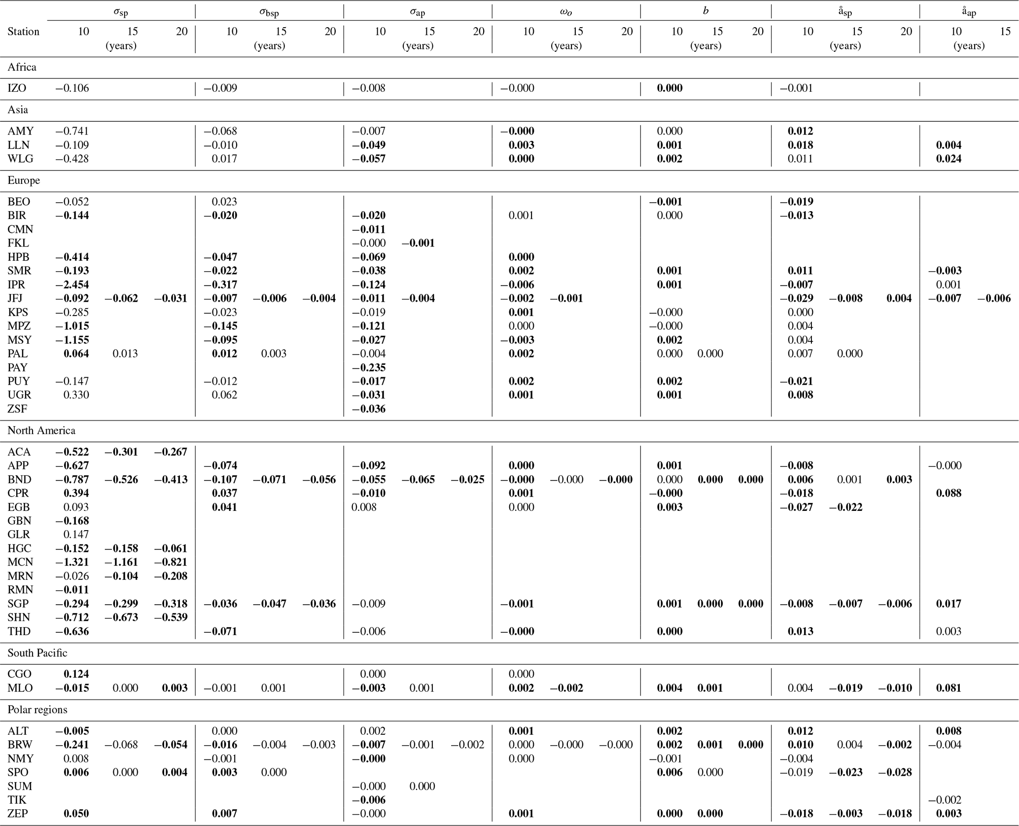
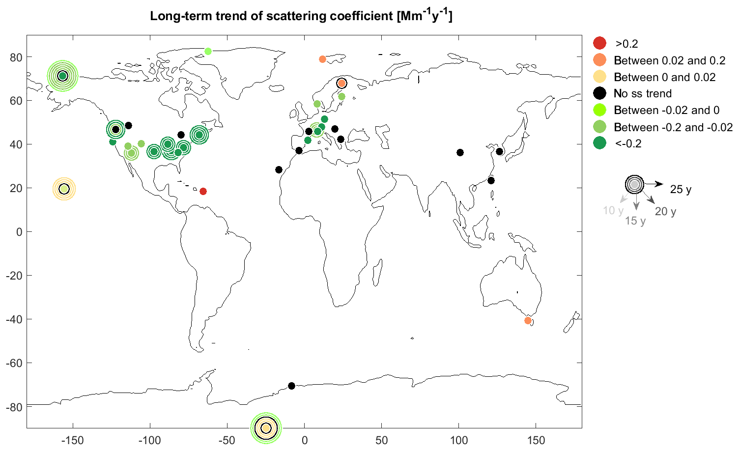
Figure 4MK trend results for the scattering coefficient. Black symbols correspond to stations with no significant trends. Green and orange symbols correspond to ss negative and positive trends, respectively. The magnitude of the trends (slope) is given by the colors as stipulated in the legend. The size of the circles is proportional to the length of the datasets, with the central dots representing the most recent 10-year trend ending in 2016, 2017 or 2018. If possible, trends for longer time periods were calculated and the larger circles denote the trends for 15 to 40 years in 5-year increments.
The σsp ss trends are predominantly negative: 20 stations have ss negative 10-year trends, 5 stations ss positive trends and 12 stations no ss trends dispersed across all continents. Eight (nine) stations with time series longer than 10 years have ss negative 15-year (20-year) trends and none (two) of the 15-year (20-year) trends are ss positive. The MK slopes range between −2.45 and +0.39 Mm−1 yr−1 with a mean of −2.19 Mm−1 yr−1. The main results are as follows.
-
Over North America, all the σsp trends for periods longer than 10 years are ss negative, and the most recent 10-year trends are generally ss negative. Three stations do not have ss trends. (1) EGB's 9-year time series does not allow for a ss trend (too short), but was included as one of only two Canadian sites. (2) MRN is an IMPROVE station on the western coast of the USA with very high humidity, leading to condensation that can disturb the humidity measurement. This makes it difficult to know whether the ss positive RH 10-year trend (Table S4) is real or due to measurement artifacts and uncertainties. If the ss positive RH trend is real, it could mask a decreasing σsp trend, resulting in a not ss trend. The time coverage for the dry σsp (σsp restricted to RH < 50 %) for MRN is too low to be representative for trend analysis. It should be mentioned that the 10-year trends for MRN ending in 2014–2018 are all not ss (see Sect. 3.2.1), so that the absence of σsp trends seems to be a real phenomenon. (3) GLR is also an IMPROVE station with high humidity. The RH trends at GLR are also not ss, and the dry σsp has a ss negative trend, similar to other stations in its vicinity.
In the previous decadal trend paper (CC2013), the trends in scattering for the arid state of Arizona were not consistent (ss positive: IBB, ss negative: SIA, PAZ, not ss: HGC, SCN). Four of the five Arizona sites (IBB, PAZ, SIA and SCB) were closed in 2010 and HGC now exhibits a ss decreasing scattering trend. MZW, the other IMPROVE station with ss positive scattering trends in 2010, also closed in 2010.
-
Most (7 out of 11) of the European sites have present-day ss decreasing σsp trends. The other four stations do not have ss trends: (1) one urban station also influenced by Saharan dust (UGR), (2) two sites in eastern European countries (KPS and BEO) and (3) a high-altitude station in the Central Range in France (PUY). The ss negative scattering trends of the Scandinavian stations have lower absolute slopes than in central Europe. PAL, the northernmost station, has a ss positive trend. PAL is geographically situated in Europe, but it can be climatologically considered an Arctic station (Schmeisser et al., 2018). PAL (slope = 0.06 Mm−1 yr−1) has a similar trend to ZEP (slope = 0.05 Mm−1 yr−1), the nearest Arctic station, with the largest ss trend in summer (JJA) when PAL is largely influenced by Arctic air masses. The increasing trend at PAL may be due to increasing biogenic secondary organic aerosol formation related to emissions from the surrounding boreal forest (Lihavainen et al., 2015a), changes in circulation patterns or a larger influence of open water with increasing concentration of sea salt aerosol.
-
Sites in the polar regions exhibit two ss positive σsp trends. In addition to ZEP and PAL, SPO also has a ss positive present-day 10-year trend but with lower slope, whereas no ss trend is found for the other Antarctic site (NMY). BRW and ALT both exhibit ss negative 10-year trends. The BRW 15-year σsp trend is not ss, whereas longer periods up to 40 years lead to ss negative trends. SPO also has very long time series but with alternating trend slopes, from ss positive for the shortest periods (10–25 years) to ss negative for the longest periods (35–40 years), with some not ss trends in between. The aerosol load is very low at BRW and SPO, leading to scattering coefficients near the instrumental detection limits, so that the measurement uncertainties are proportionally larger than for middle-latitude stations.
-
CPR, a site on the Caribbean island of Puerto Rico, has a ss positive σsp trend. At CPR, the largest scattering trend is found in summer and the scattering trend of the PM10 trend is 5 times larger than the PM1 trend. The most probable explanation is increased Saharan dust transport over the Atlantic Ocean; more dust transport has been reported at an IMPROVE site in the Caribbean (Hand et al., 2017, 2019).
-
The only two stations representing the Pacific region are MLO and CGO. The recent MLO 10-year σsp trend is ss decreasing, the σsp 15-year trend is not ss, whereas the trends for the longer time periods (20–30 years) are ss positive (see Fig. 2). In the previous decadal trend paper (CC2013), MLO exhibited a ss positive trend for the 10-year period ending in 2010. MLO σsp trends changed from previously ss positive to currently ss negative trends. The recent 10-year trend at CGO is found to be positive and quite homogeneous with the seasons, with fall being the only season without a ss trend.
-
The σsp trends are mostly (70 %) not ss for stations at middle to high altitudes. From the 10 stations higher than 1100 m a.s.l., only SPO in Antarctica has a present-day ss positive 10-year trend and only JFJ in the European Alps, HGC in Arizona and GBN in Nevada exhibit ss negative 10-year trends. In contrast, only 26 % of the stations lower than 1100 m a.s.l. do not have ss trends. New particle formation (NPF) and growth are favored at high altitudes (> 1000 and up to 5000 m) due to low temperatures, high solar radiation and low pre-existing particle concentrations, leading to limited condensational sinks for nucleation precursor gases (Sellegri et al., 2019). This higher frequency of nucleation at high altitude leads to a high contribution of secondary particles to the total number concentration that largely contributes to the total scattering coefficient. The decreasing σsp trends from anthropogenic pollution in the planetary boundary layer can, consequently, be masked by the presence of NFP at high-altitude stations.
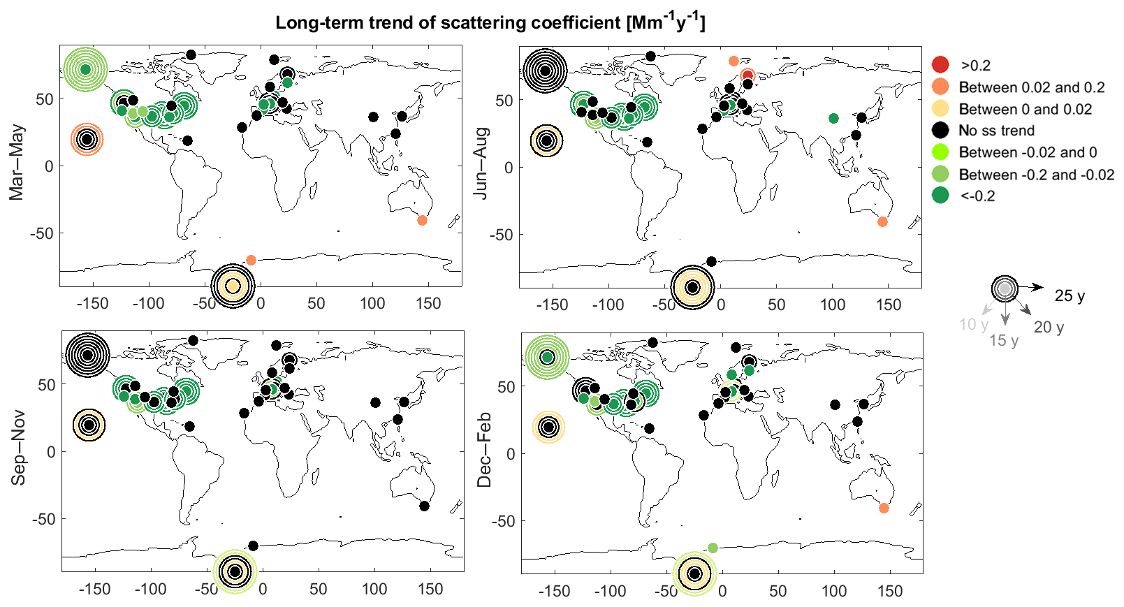
Figure 5Seasonal results of the MK trend of the scattering coefficient. Other details same as Fig. 4.
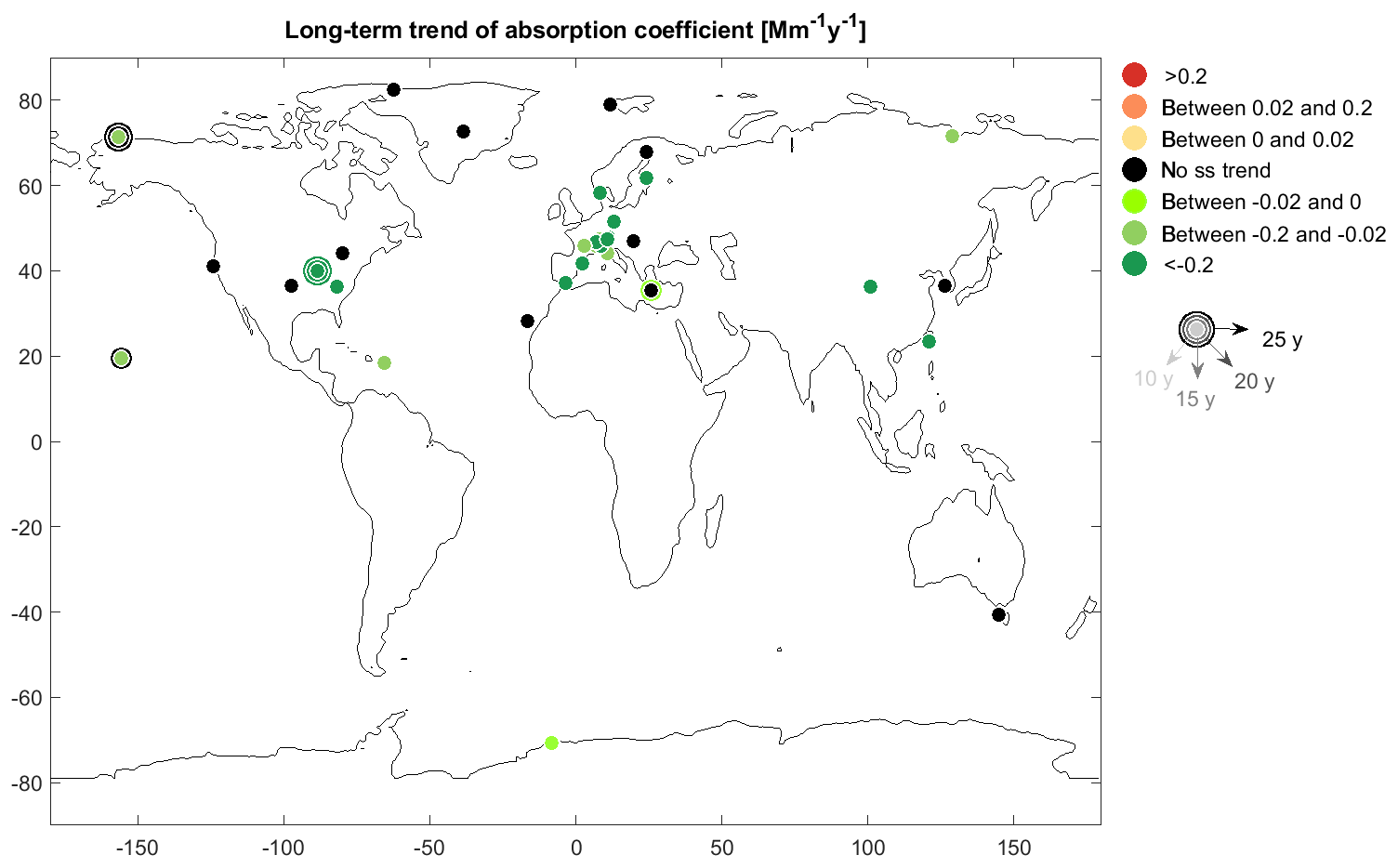
Figure 6MK trend results for the absorption coefficient. Other details same as Fig. 4.
The seasonal MK results for σsp are presented in Fig. 5. Spring is the season with the largest number of ss decreasing trends and winter the season with the lowest. ZEP and PAL exhibit ss positive trends only in summer and BRW has ss negative trends only between December and May. The SPO annual trend is ss positive, whereas it is not for NMY. Both Antarctic stations exhibit, however, a coherent seasonality with ss positive trends only in spring. While the 25- and 30-year trends at MLO are all ss positive, with the largest slope in spring when MLO is influenced by Asian long-range transport (CC2013), the most recent 10–20-year trends are not ss for the individual seasons.
3.1.2 Absorption coefficient
The analysis of σap long-term trends has been performed on 33 datasets (see Fig. 6 and Tables 2 and 3). The long-term trends are ss decreasing (21 stations) or not ss (12 stations) for all stations around the world, leading to a mean decreasing trend of −3.05 Mm−1 yr−1. No ss σap positive trends are measured for any of the stations. The other main results are the following.
-
In North America the number of σap datasets is much lower than the number of σsp datasets (IMPROVE sites do measure aerosol absorption, but with a different instrumental setup; White et al., 2016). From the five sites with long-term aerosol absorption, APP and BND, two continental rural sites, and the marine Caribbean island (CPR) station have ss negative trends. The other three stations representing the continental rural USA (SGP, EGB) and marine western coast of the USA (THD) exhibit not ss trends in σap.
-
In Europe, most (12 stations) of the 10-year σap trends are ss negative. Only three stations, one Scandinavian (PAL), one eastern rural continental (KPS) and one coastal Mediterranean (FKL) station exhibit no ss trends. The 15-year σap trends at JFJ and FKL are ss negative.
-
In Asia, both the high-altitude stations of LLN in Taiwan and WLG in China exhibit annual ss decreasing σap trends. The South Korean coastal station of AMY has no ss annual trend.
-
For the polar regions, the Antarctica site of NMY, the American Arctic site of BRW and the Russian Arctic site of TIK have slight ss negative σap trends, whereas SUM, ALT and ZEP have no ss trends. Thus, there is no common clear σap trend in the polar regions.
-
In the southwestern Pacific, the high-altitude station of MLO has a ss decreasing trend for the last 10 years but no ss trend for the last 15 years, whereas the coastal station of CGO in Australia exhibits not ss σap trends.
-
In contrast to the σsp trends, σap trends at high-altitude stations (> 1100 m a.s.l) are mostly (6 out of 8) ss decreasing; the trends at the other two high-altitude stations are not ss.
The seasonal trends are more strongly negative and more ss in spring than in summer (see Fig. S3). Winter is the season with the smallest number of ss decreasing trends in Europe (only 2∕15) and with the only ss positive trend (ZSF), the others being not ss, whereas fall seems to be the season with the lowest ss trend in North America.
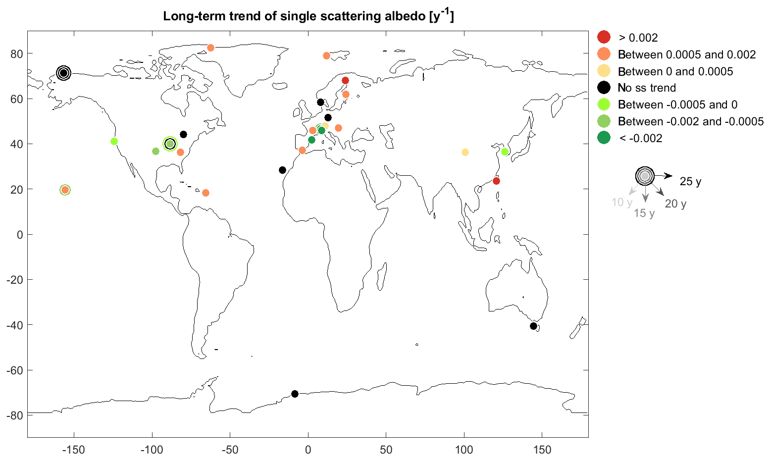
Figure 7MK trend results for the single scattering albedo. Other details same as Fig. 4.
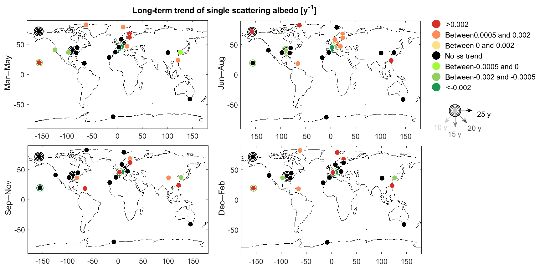
Figure 8Seasonal results of the MK trend of the single scattering albedo. Other details same as Fig. 4.
3.1.3 Single scattering albedo
As described under Sect. 2.4, ω0 trends have to be considered with greater caution since the σap absolute values suffer from a certain uncertainty related to filter-based absorption photometer artifacts.
The ω0 trends depend directly on both the magnitude and the sign of the σsp and σap trends. If expressed in % yr−1, a σap trend larger (smaller) than the σsp trend will result in an increasing (decreasing) ω0 trend, respectively (see Fig. S8 and the related estimation of ω0 uncertainty due to measurement and Cref errors). The ω0 trends are consequently much more diverse than the σsp and σap trends with 52 % of ss positive (relatively more scattering), 22 % of ss negative (relatively more absorption) and 26 % not ss trends (see Fig. 7 and Table 2). One peculiarity is that all ω0 ss negative trends are found between latitudes 30 and 50, but this is perhaps due to the low spatial coverage outside of North America and Europe. The main results are the following.
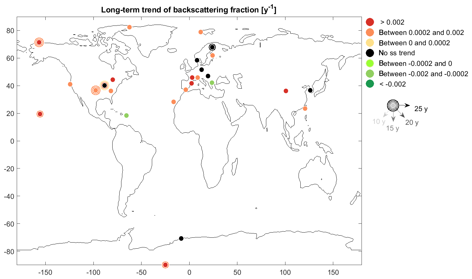
Figure 9MK trend results for the backscattering fraction. Other details same as Fig. 4.
-
The ω0 is decreasing at three stations in North America (BND, SGP and THD), whereas APP and CPR exhibit ss positive ω0 trends. The CPR ω0 increasing trend can perhaps be related to increased Saharan dust load. The seasonal ω0 trends at CPR are, however, ss not only in summer when Saharan influence is greatest, but for every season except spring (Fig. 8). EGB has no ss trend.
-
European stations exhibit ss increasing ω0 trends at the urban station of UGR and at most eastern and Scandinavian stations (KPS, SMR, PAL) and at the mid-altitude station of HPB. These ss positive ω0 trends in eastern and northern Europe are strongest in summer (Fig. 8), when MEL and BIR are also ss positive, and weakest in winter when only PAL is ss positive (possibly related to increased particle formation from biogenic emissions, as mentioned above). In central Europe, JFJ, IPR and MSY have ss negative ω0 trends for the entire year as well as for all seasons. PUY, a station at 1465 m in France's Central Range, has a ss positive annual trend due to strong positive trends in fall and winter, even if a strong ss negative trend is found in summer. Because the site is located at a mid-range elevation (1465 m a.s.l.), PUY has a large probability of being influenced by different air masses as a function of the season, with a large impact of the planetary boundary layer in summer (Collaud Coen et al., 2018; Hervo, 2013).
-
The high-altitude stations of LLN and WLG in Asia have strong and weak ss positive annual ω0 trends, respectively. This pattern is also observed for all seasonal trends at LLN, but only in fall at WLG. The coastal station of AMY has a ss decreasing annual ω0 trend that is due to decreasing trends in MAM, SON and DJF. AMY is located in an agricultural and touristic region that is influenced not only by these regional aerosol sources (e.g., traffic, field burning), but also by long-range transported plumes with high aerosol load.
-
The Arctic stations of ALT and ZEP have ss positive ω0 annual trends, which are due to ss positive trends from December to August for ALT and from December to May for ZEP. The two polar stations (BRW and NMY) exhibit no ss ω0 annual trends, although there is a ss positive trend in summer at BRW for the most recent 10-year time series.
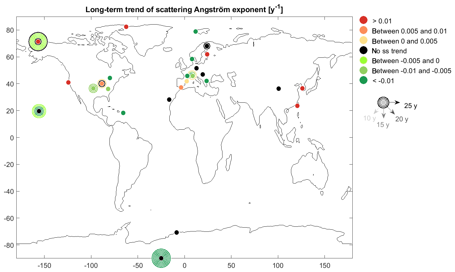
Figure 10MK trend results for the scattering Ångström exponent. Other details same as Fig. 4.

Figure 11MK trend results for the absorption Ångström exponent. Other details same as Fig. 4.
3.1.4 Backscattering fraction and scattering Ångström exponent
The present-day trends for the backscatter fraction b are mostly ss positive (65 %) across all regions (Fig. 9 and Table 2). This suggests a shift in the size distribution towards smaller accumulation-mode aerosol. The two stations with ss negative trends are CPR in Puerto Rico and BEO, located on a summit in the Balkan range. Not ss trends are mostly found in eastern and northern Europe (KPS, MEL, BIR and PAL), in Antarctica (NMY), as well as at BND and AMY for the last 10 years. The Arctic sites (ALT, BRW and ZEP) all exhibit ss positive b trends. CPR's seasonal trend is ss negative only in fall; trends in b for the other seasons at CPR are not ss (see Fig. S4). Similarly, the BEO b seasonal trend is ss negative only in summer, and not ss otherwise. PAL has ss positive b trends in spring and summer and ss negative b trends for fall, leading to an annual not ss trend.
The scattering Ångström exponent (åsp) trends exhibit a higher variability than the trends in other parameters, with 33 % of ss positive trends, 37 % of ss negative trends and 30 % of not ss trends (Fig. 10 and Table 2). There are ss positive and negative trends in North America, Europe and the polar regions, and the various trends cannot be attributed to specific regions or environments. It should be recalled, however, that åsp is affected by higher uncertainties (see Sect. 2.3) that may contribute to the larger observed variability. The seasonal results also exhibit high variability, with summer being the season with the least number of ss åsp trends (10 out of 26 sites), while spring and fall are the seasons with the largest number of ss positive and negative trends in åsp (8 out of 26 sites), respectively (see Fig. S5).
3.1.5 Absorption Ångström exponent
The number of stations with long-term åap measurement is low, with only 14 time series available. Seven stations situated in various geographical regimes exhibit ss positive trends (Fig. 11 and Table 2): polar regions (ALT and ZEP), a Caribbean coastal station (CPR), a rural continental North America station (SGP), and high-altitude stations in the remote Pacific (MLO), in continental (WLG) and in coastal (LLN) Asia. SMR and JFJ, two stations in Europe but with very different environmental footprints and altitudes, exhibit ss decreasing åap trends; the six other stations, consisting of three coastal and two continental sites, have no ss trends.
While CPR and SGP åap trends are ss positive and JFJ ss negative for all four seasons, the other stations exhibit higher variability as a function of the meteorological seasons (see Fig. S6). The absorption Ångström exponent is principally a function of the particle chemical composition and material properties, but its assignment to an aerosol type is not uniquely defined and also depends on the particle size, with larger particles corresponding to lower åap values (Liu et al., 2016; Schmeisser et al., 2017). For example, åap>2 corresponds to mineral dust in the case of big particles and to brown carbon in the case of small particles. In contrast, åap<1 corresponds to large particles with small absorption like sea-salt-dominated aerosol in the case of big particles and to black carbon (BC)-dominated aerosol in the case of small particles. Following these observational constraints, the JFJ and SMR aerosol tends to represent the category “mixed BC/BrC” according to Schmeisser et al. (2018). CPR absorption has a strong contribution from mineral dust and sea salt, whereas at MLO, SGP, ALT and ZEP contributions to absorption are from mixed sources, including various light-absorbing carbon species and dust. Ideally, direct chemical composition measurements would provide more precise information on the aerosol type, but the necessary chemical composition measurements are not yet readily available at many sites.
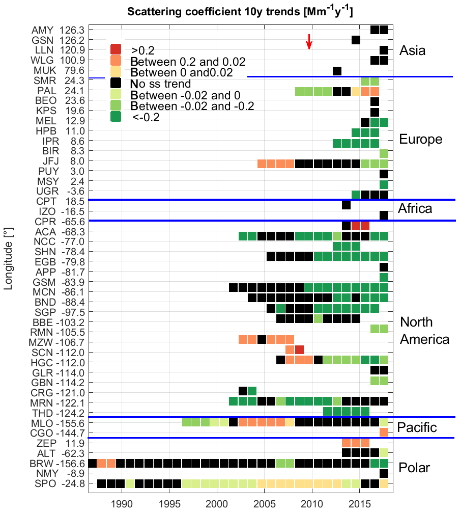
Figure 12Time series of sequential 10-year σsp trends as a function of station longitude. Stations in the South Pacific and in the polar regions were grouped for clarity. The red arrow indicates the end of the time periods covered in CC2013.
3.2 Time evolution of 10-year trends
The previous section describes the present-day trends for different periods extending from 10 to 40 years. Another interesting analysis is to follow the evolution of the trends in time and space. For this purpose, all the possible 10-year trends were computed and plotted as a timeline for each station. In what follows each point on the timeline represents a 10-year trend ending in the year it is located on the graph. For example, in Fig. 12 the two black points for AMY represent the 10-year trends covering the periods 2008–2017 and 2009–2018, respectively. These timelines can be presented as a function of the latitude, longitude, altitude or environment. Depending on the results, the most interesting representation has been chosen for each parameter.
3.2.1 Scattering and backscattering coefficients
Figure 12 presents the σsp 10-year trend timelines as a function of the longitude of the stations. The σbsp 10-year trend timelines are similar to the σsp trend timelines (see Fig. S7). The polar stations (in both the Arctic and Antarctic) have been gathered to the bottom of the figure just after the two Pacific stations of MLO and CGO. The main result is that the sites in eastern and central North America (longitude between −68 and −112∘) have ss negative σsp 10-year trends ending after 2009–2012 regardless of their altitude (200–2200 m a.s.l.) and their environments. This is a clear signature of continental-scale modification due to air quality regulations, and this very clear feature relates to the sulfate-dominated aerosol in the eastern USA and to large SO4 reductions in power plant emissions (Hand et al., 2014; McClure and Jaffe, 2018). Almost all the σsp 10-year trends in the southwestern USA (MZW, SCN and HGC) ending before 2011 are ss positive, as published in the previous trend analysis (CC2013). MLO also exhibits ss positive trends for the same period. These four stations are also high-altitude sites (2000–3400 m), so that it is possible that all of them were influenced by long-range transport of highly polluted air masses from Asia (CC2013). It is further interesting to note that the high-altitude site JFJ (3580 m) in Europe also exhibited a ss positive 10-year trend ending in 2005–2008.
The evolution of the European σsp 10-year trends does not show a clear time for trend modification as is seen in North America, probably due to variable timing in implementation of abatement policies in each individual country. Apart from PAL (which can be considered, to some extent, to be a polar station), the σsp 10-year trends in Europe ending after 2008 are all ss negative or not ss. The four stations in Asia do not have ss trends ending in the last 5 years. The two African stations exhibit no ss trend. For polar sites, BRW, ALT and NMY have mostly not ss trends, whereas SPO exhibits alternating ss positive and negative trends, with the oldest 10-year trends being not ss. In contrast, ZEP exhibits positive trends for all three 10-year periods, which is similar to the 10-year trends at PAL for the same time periods. Due to the very low aerosol concentrations at these sites and, thus, larger measurement uncertainty, it is difficult to interpret the evolving σsp polar trends. They could be related to increased influence from the boreal forest and/or changed circulation patterns modifying the sea/ice influence.
The GSN dataset only covers 8 years, with some missing periods due to the destruction of the station by a typhoon. Due to the very low number of long-term measurements in Asia, GSN was included in this study. While GSN σsp summer trends are not reliable (low data coverage and issues in humidity control), the ss negative winter–spring trends corresponding to the dry season are valid and in line with the PM10 decreasing trends in Korea (Kim and Lee, 2018; Nam et al., 2018).
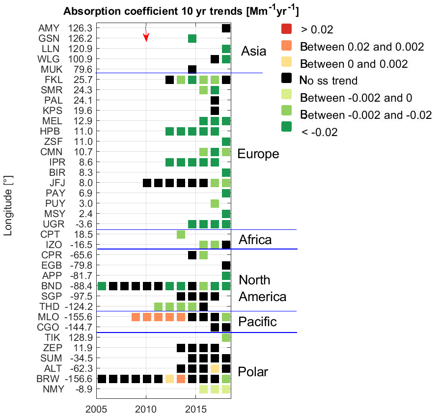
Figure 13Time series of sequential 10-year σap trends as a function of station longitude. The red arrow indicates the end of the time period covered in CC2013.
3.2.2 Absorption coefficient
The lengths of the σap time series are much shorter than for σsp (Fig. 13). This means that the oldest 10-year trends cover the period 1998–2007 (BRW and BND), followed by MLO (2001–2010) and JFJ (2002–2011). For these four stations, the most recent 10-year trends are either not ss or ss negative. The present-day (i.e., trends covering 2009–2018) ss negative 10-year trends (JFJ, BND, MLO and BRW) are preceded by not ss trends. The σap 10-year trend evolution of each station is usually homogeneous with either ss negative or not ss 10-year trends in Asia, Europe, Africa and North America. ALT σap 10 years ending in 2017 is ss positive. The BRW polar station and MLO high-altitude station exhibit also some ss positive 10-year trends ending between 2010 and 2014. Unfortunately, only MLO has a long enough σap time series to compare with the ss positive σsp 10-year trends at high-altitude sites (Fig. 12). At MLO, the series of ss positive σsp 10-year trends ended in 2008, while the series of ss positive σap 10-year trends occurred for the period ending 2009–2013.
Figures 12 and 13 suggest that mid-latitude σsp and σap sequential 10-year trends were ss positive for some periods between 2000 and 2013, followed by not ss trends and ending in the present day with ss negative trends. The evolution from increasing to decreasing σsp and σap trends appears to be not simultaneous, with the σsp inflection points occurring some years before those for the σap trends. The sparse number of stations with long enough time series does not allow generalization of this result.
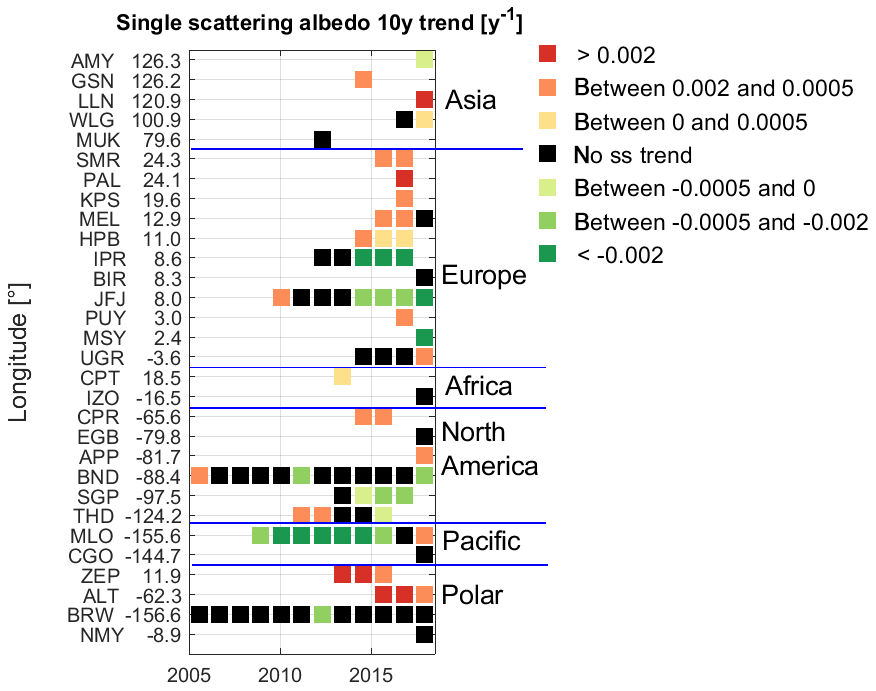

Figure 15Time series of sequential 10-year b and åsp trends as a function of station longitude. The red arrows indicate the end of the time period covered in CC2013.
3.2.3 Single scattering albedo
Because it is limited by the length of σap time series, the ω0 10-year trend evolution also only covers the last decade. The following results can be seen in Fig. 14.
-
All stations at longitude > 10∘ have ss positive ω0 10-year trends except for AMY, which exhibits a ss negative 10-year trend ending in 2018, and MUK with a not ss 10-year trend ending in 2013. For European sites, ss positive ω0 10-year trends exist for all stations at latitude > 46.8∘, apart from BIR, which has a not ss trend ending in 2018. This suggests that the decreasing σap trends in Asia and in eastern and northern Europe are proportionally larger than the decreasing σsp trends.
-
The central and western European sites exhibit mostly ss negative or not ss ω0 10-year trends. At JFJ and IPR, a shift from not ss to ss negative 10-year trends occurred in 2013–2014. The JFJ time series is moreover long enough to monitor a ss positive ω0 10-year trend ending in previous years (2010). The urban station of UGR in Spain exhibits an increasing trend in ω0 (decrease in contribution of absorbing aerosol) for the most recent 10-year period (2009–2018), possibly related to long-term effects of the 2008 financial crisis (e.g., Lyamani et al., 2011).
-
In North America, the ω0 10-year trends ending after 2013 are ss negative or not ss, apart from CPR in Puerto Rico and APP. The sites with the longest series of ω0 10-year trends (BND and THD) exhibit ss positive trends followed by not ss and ss negative trends. In contrast, MLO ω0 10-year trends shifted from ss negative trends (10-year trends ending in 2010–2015) to not ss trends (10-year trends ending 2017) to a ss positive trend in 2018. This is consistent with the observed increase in σap 10-year trends ending in 2010–2012.
-
The two polar sites of BRW and NMY exhibit mostly not ss ω0 10-year trends, whereas ALT and ZEP, similar to northern European sites, exhibit ss positive ω0 for all the 10-year trends.
3.2.4 Backscattering fraction and scattering Ångström exponent
Both the b and åsp 10-year trends in Asia and Africa exhibit similar 10-year trend patterns that are either ss positive or not ss (Fig. 15). In this context, similar means that the b and åsp trends are never ss when opposite signs of the slope are observed. These results suggest that particle average size tends to decrease at the Asian and African sites. In Europe, b and åsp 10-year trends have a majority of ss negative or not ss trends in the northeast (longitude > 10∘). At lower European longitudes, there is a discrepancy between b and åsp 10-year trends, with IPR, JFJ and PUY having opposite ss trends for b and åsp, b trends being often ss positive and åsp trends often ss negative. The discrepancy in the signs of the trends for b and åsp may be related to shifts in both the fine and coarse modes of the aerosol size distribution – this is discussed more below (see Sect. 4.2).
In North America, the b 10-year trends ending after 2012 are almost all ss positive, whereas the previous 10-year trends are ss negative at BND and MLO. As in western America, one can see discrepancies in the sign of the slope for b and åsp 10-year trends, with APP, CPR, MLO, SGP and THD having at least one 10-year period with opposite signed ss trends. Also, as in western Europe, the b trends are usually ss positive and the åsp trends ss negative. BND records four 10-year periods with opposite ss trends. In contrast to the other stations, BND åsp trends are ss positive, while BND b exhibits ss negative trends.
In the polar regions, the b 10-year ss trends ending after 2014 are all ss positive, whereas the older trends are primarily ss negative. Here again, the discrepancy between b and åsp 10-year trends is large, with all the 10-year b and åsp trends for ZEP and ALT being ss with opposite signs. In contrast, BRW exhibits trends with the same sign for both parameters that can be interpreted as an increase in average particle size for early years followed by a decrease after 2014.

Table 3Number of trends analyzed for each parameter, of ss cases for each trend analysis method, of trends with similar statistical significance in MK, GLS/day and LMS/log, of trends with similar statistical significance for all five methods, of trends with at least GLS/day or LMS/log ss similar to MK, and of trends with no agreement between these two methods and MK ss.

3.2.5 Absorption Ångström exponent
The åap time series are not very long, because the first generation of absorption photometers used either white light or only one wavelength (Fig. 16). The longest time series of åap begins in 2002 at JFJ and exhibits a continuous ss åap decrease. Similar to the results for JFJ, most of the stations have consistently ss negative (JFJ, SMR), ss positive (ALT, ZEP, IPR, SGP, WLG, LLN, MLO and CPR) or not ss 10-year trends (TIK, BRW, THD, APP, GSN, MUK and CPT). The not ss trends of TIK and GSN may be due to datasets shorter than 10 years.
3.3 Comparison of the trends among methods
As described under Sect. 2.5, the long-term trends were computed with three methods (MK, GLS and LMS), where GLS was used on both daily and monthly medians and LMS with and without taking the logarithm of the monthly medians. These methods are thereafter called GLS/day, GLS/month, LMS/log and LMS/lin, respectively. Tables S2 and S3 give the GLS/day and LMS/log results for all parameters and stations. Table 3 presents an overview of the number of present-day 10-year trends that are ss with each method. For the reasons described in Sect. 2.5.1, MK is considered to be the most appropriate method for aerosol optical parameters. The agreement between the three methods used in CC2013 (MK, GLS/day and LMS/log) and between all five methods are then also reported in Table 3, as well as the number of cases with either GLS/day or LMS/log agreement with MK and with both GLS/day and LMS/log disagreement with MK. The following conclusions can be derived.
-
Generally, the trends computed by the various methods agree very well with one another. Among all parameters, all stations and all periods, none of the present-day trends presents ss results with opposite slope for different methods. In all cases, the differences among methods relate either to the degree of the ss or to the sign of the slopes for not ss trends. This implies that the main conclusions of this study would not have been fundamentally different if the other methods were used.
-
GLS applied on daily medians is the method that has the largest number of ss trends for all parameters.
-
The three methods applied on monthly data have a lower number of ss trends for all the computed parameters (ω0, b, åsp and åap).
-
The three methods used in 2013 have similar statistical significance (comprising cases with no ss trend) in 44 % to 86 % of the cases, whereas the five methods used here exhibit consistency in 37 % to 82 % of the cases. The measured parameters, which are less uncertain than the calculated parameters, always exhibit the largest agreements amongst the methods (> 69 % for the three methods used in 2013 and > 63 % for the five methods utilized here). ω0 is always the parameter with the largest dissimilarity among the methods and σbsp the parameter with the largest similarity among methods.
-
The MK statistical significance is similar to at least one of the methods applied in 2013 in more than 90 % of the cases for all of the parameters apart from ω0 (88 %) and åap (78 %). This lower level of agreement can be explained by the fact that ω0 and åap are almost normally distributed, so that the use of the LMS/log is not appropriate.
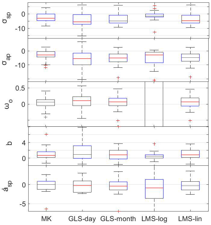
Figure 17Median, interquartile ranges and whiskers of the slopes in % yr−1 computed by the five methods for the scattering coefficient, the absorption coefficient, the single scattering albedo, the backscattering fraction and the scattering Angström exponent. The outliers are not always visible in the figure for the purpose of clarity.
The boxplots of the slopes computed by the various methods (Fig. 17) show first that the application of the logarithm to transform to a normal distribution for ω0 and åap (not shown) is not suitable and leads to very large interquartile ranges. While the measured parameters are clearly not normally distributed, the derived parameters usually have distributions that more closely approximate normal distributions. No systematic rule could be deduced, since the distributions of each computed parameter largely depend on the individual stations. It seems however that ω0 and the Ångström exponents are closer to the normal distribution than to the lognormal distribution.
The Sen slope estimator applied to the variance-corrected pre-whitening (Wang et al., 2015) leads, in almost all cases, to a median of the slope nearer to zero than the other methods. The VCTFPW method was developed specifically to get rid of the falsely increased slope by the trend-free pre-whitening process (Collaud Coen et al., 2020a). The LMS/log method sometimes results in lower absolute slope medians, and this effect is probably due to the almost normal distribution of the data (= log of the monthly median). Both the GLS (GLS/day and GLS/month) and LMS/lin methods lead to higher absolute slopes, probably due to misuse of statistical methods developed for normally distributed data.
The GLS/day method leads to a broader range of slopes than the GLS/month method. This larger variance may be due to (1) the larger variability of daily data, leading to a less distinct seasonal cycle and, consequently, to a worse fit of the seasonal variation and (2) a higher autocorrelation in the daily time series with, possibly, an autocorrelation order larger than one.
4.1 Considerations related to measurement humidity
As explained in the instrumental section, GAW protocol suggests that the σsp and σbsp be measured at low and controlled humidity, and that is the case for almost all stations considered here, except for those in the IMPROVE network which measure at ambient conditions due to their different monitoring goals. Temporal cycles and variations of RH with time are observed in a number of datasets. There are also some clear breakpoints in measurement RH that have been identified at several stations (e.g., an insulating jacket was installed on the nephelometer at THD in late 2012, resulting in a clear decrease in sample RH due to warmer nephelometer temperatures). It is evident that high RH will enhance particle diameters and, consequently, increase σsp, σbsp and ω0 while resulting in decreased b and åsp. This particle diameter enhancement depends not only on the RH values, but also on the particle hygroscopicity, which is a function of the aerosol size distribution and chemical composition.
Similarly to the previous aerosol optical property trend study (CC2013), dry σsp was calculated by removing data when measurement RH was higher than 50 % in order to minimize the impact of aerosol hygroscopicity on the scattering trends. However, hygroscopic growth can occur for RH < 50 %; for example, for sea salt aerosol, up to 25 % of the scattering could be due to water at RH = 40 % (e.g., Fig. 5 in Zieger et al., 2013). The confounding effects of aerosol water impact the reported scattering values and, hence, the trends presented here to a greater or lesser extent. The effect of hygroscopic growth at RH < 50 % on the reported trends would depend on the temporal variability in sample RH, composition and size; investigating the interactions amongst those parameters is beyond the scope of this study.
For this study, if RH was frequently larger than 50 % at a station, relationships between RH and aerosol parameter trends were analyzed as follows. In the case of the RH trend being not ss, the aerosol parameter trends were considered to be independent of the RH variation. In the case where a ss RH trend was detected (see Table S4 in the Supplement), an attempt was made to try to determine the influence of RH trend on each aerosol parameter by considering the following situations: (1) if all aerosol trends follow the RH trends, (2) if σsp at all measurement RH and dry σsp trends are similar, and, finally, (3) the features of σap trends, which are less likely to be influenced by long-term RH variation. The distinct patterns exhibited by the evolution of the 10-year trends were very helpful in this analysis. Below we describe the assumed implications for scattering trends at sites where trends in RH were observed for several cases.
-
Trends in RH are the opposite of both σsp and σbsp trends: this implies that the aerosol optical property trends are real and not influenced by humidity (SMR, SHN, MRN).
-
Trends in RH are ss, but trends in σsp are not ss: this implies that the absence of statistical significance for the σsp trends is real if the slopes of the RH and σsp trends have the same sign (IZO, LLN) or can be partially induced by the RH trend if the slopes have opposite signs (EGB, PUY, UGR).
-
Trends in RH and σsp are similar, the overall and dry (RH < 50 %) σsp trends are similar, and σsp and σap exhibit similar trends: this implies that the σsp trends are probably influenced by RH but also have an intrinsic aerosol trend (APP, BIR, MZW, SGP).
-
Trends in RH and σsp are similar, but the dry (RH < 50 %) and overall σsp trends are dissimilar and the trends in σsp and σap are also dissimilar: this implies that the RH influence is major (THD, CPR). THD and CPR are coastal stations with a dominant influence of sea salt. At THD on the North America western coast, RH, σsp and σbsp trends are ss decreasing, whereas b and åsp trends are ss increasing and σap trends are also ss decreasing but with lower slope and ss than σsp. Further, the PM1 trends were less ss and exhibited much lower slopes, suggesting that the large sea salt particles are probably sensitive to the RH decrease, leading to the decreasing σsp trend. The 10-year trends show that RH decreasing trends are particularly important until 2015 and likely explain the ω0 ss positive 10-year trends ending in 2012 and 2013. At CPR, a coastal site in the Caribbean, RH, σsp and σbsp trends are ss increasing, but the σap 10-year trends do not have the same shape or statistical significance as the σsp trends. As observed at THD, the PM1 trends at CPR are less ss and have much lower slopes than PM10 trends.
As mentioned in the instrumental section, RH trends measured by the nephelometers have to be considered with caution. Because the measurement RH is only a secondary parameter, the instrument humidity sensors are typically not maintained or calibrated with the same care as the scattered light detectors. The influence of humidity variations on the optical property trends presented here can generally be considered to be low, apart from the cases of very hygroscopic particles like sea salt (e.g., at THD and CPR). A better knowledge of the particle hygroscopic growth at low RH (< 40 %) would be valuable in order to interpret σsp and σbsp trends as well as trends in ω0, b and åsp.
4.2 Particle size trends
Both the scattering Ångström exponent and the backscattering fraction are indicators of the particle's average size, with the general interpretation that lower values of b and åsp correspond to the presence of larger particles albeit at different parts of the aerosol size distribution (Collaud Coen et al., 2007). However, the relation between b and åsp is not uniquely defined for several reasons. First, the scattering efficiency has an oscillating response to particle size rather than a constant increase. Second, the measured particle size distribution is usually composed of several modes. Since the sensitivity of scattering to the mode depends on the size parameter (proportional to the ratio diameter–wavelength), b (here usually taken at 550 nm) and åsp (here usually computed with the 450–550 nm pair) do not always exhibit similar sensitivity to the various size modes. Further, the extinction Ångström exponent (analogous to åsp) was found to be more sensitive to fine-mode volume fraction if computed from long wavelengths and to fine-mode effective radius if computed from short wavelengths (Schuster et al., 2006). Lastly, the relation between b and åsp also depends on the refractive index and consequently on the absorption coefficient (Hervo, 2013): for a constant particle diameter, an increase in the refractive index real part will decrease åsp but increase b.
In this analysis, some stations exhibit b and åsp trends with the same sign (BRW, CPT, SMR, LLN, SPO, UGR), while for other stations b and åsp trends are in opposite directions (ALT, APP, BEO, BND, EGB, JFJ, MLO, MSY, PAL, PUY, SGP, SPO, ZEP). The plots showing the evolution of the 10-year trends (Fig. 15) demonstrate that b and åsp can exhibit either similar or opposite trends depending on the considered periods (CPR, IPR, MLO, THD). The plots showing the evolution of the 10-year trends also suggest that the variations of the 10-year slopes are often identical in sign but with different magnitude (e.g., shifted towards larger trend values for b; see for example MLO, Fig. 18).
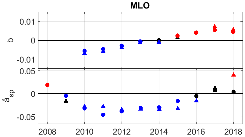
Figure 1810-year slopes of b and åsp at MLO. Ss negative and positive trends are plotted in blue and red, respectively. Not ss trends are plotted in black. The dots correspond to PM10 and the upwards triangles to PM1.
We can attribute both b and åsp ss positive trends (ALT, BRW, SMR, LLN, THD, UGR) to a shift in the accumulation mode towards smaller sizes and a decrease in the coarse-mode particle concentration. In contrast, ss negative trends (BEO, CPR) for both b and åsp suggest a shift to bigger sizes, specifically an increase in the coarse-mode particle concentration and perhaps also a shift towards larger diameters of the accumulation mode. At a boreal forest site in northern Europe (SMR), size distribution data suggest that seasonal variation of b and åsp was caused by a shift in the accumulation mode and not by changes in the coarse-mode fraction (Luoma et al., 2019). Trends towards smaller particle sizes might be due to an increase in near-anthropogenic sources of pollution, to an increase in new particle formation, to a decrease in long-range transport of anthropogenic pollution, to increased scavenging of larger particles due to changes in atmospheric conditions, to a modification of atmospheric chemistry (Banzhaf et al., 2015) or to a change in both primary and secondary natural aerosol (e.g., an increase in biogenic secondary aerosols and their precursors as demonstrated by Ciarelli et al., 2019). Trends towards bigger particles can relate to a decrease in near-anthropogenic emissions, to larger influence of mineral dust caused by variation in desert emissions or dust transport, to changes in agricultural activities or to an increase in humidity.
For stations with opposite b and åsp trends, the chemical composition may play an important role in identifying reasons for the changing trends. It is however out of the scope of this paper to study these kinds of dependencies.
Table 4Overview of the aerosol optical property decadal MK trends ending between 2016 and 2018 for all the stations and per continent/region of the world.

4.3 Single scattering albedo trends
The single scattering albedo is the most important variable determining the direct radiative impact of aerosol, so that its trend analysis – derived for the first time for a large number of stations – has a high relevance. The filter-based absorption photometer artifacts lead to uncertain absorption absolute values that have no effect on σap trends but impart higher uncertainties to ω0 trends. The results of ω0 trends depend directly on the relative values of σsp and σap trends. The global picture is nuanced, with about half of ss positive, one-fifth of ss negative and one-fourth of not ss trends leading to an annual positive median trend of 0.02 % yr−1 (Table 4). The medians of ss trends are increasing in Asia, in the Arctic and in the Pacific but decreasing in Europe and North America. The largest median slopes are found in Asia and in the Pacific (+0.13 and 0.14 % yr−1, respectively), whereas the decreasing median slopes in other regions are relatively small (< 0.01 % yr−1). The beginning of the decrease in the aerosol burden varies with region; the earliest decrease is found in Europe in the 1980s (Tørseth et al., 2012), followed by North America in the 1990s (Bodhaine and Dutton, 1993; Hand et al., 2012) and by Asia some 10–15 years ago (Sogacheva et al., 2020; Zhao et al., 2019; Paulot et al., 2018). The median slope of the ω0 trends seems to be proportional to the length of the mitigation efforts, which for some relevant pollutants (e.g., black carbon, SO4 and NOx) are still ongoing. In Europe, the diversity of the timing of abatement policies with earlier impact in western Europe than in eastern Europe (Vestreng et al., 2007; Crippa et al., 2016; Huang et al., 2017) is also directly visible in the decreasing and increasing ω0 trends (Figs. 7 and 14), respectively.
These results suggest that policy regulations induced first a ω0 increase (cooling effect) and, in a second phase, a ω0 decrease (warming effect). The Emission Database for Global Atmospheric Research (EDGAR V4.3.2) (easy accessible via https://eccad.aeris-data.fr/, last access: 20 July 2020) shows that both the BC and SO4 emissions decreased rapidly during the 1990s and that currently emission reductions of SO4 are larger than the reductions for BC. From this we conclude that the reduction of primary particles, such as BC, leads first to the ω0 increase, whereas the reduction of SO4, a precursor of secondary particle formation, tends to result in a ω0 decrease. Moreover, emission changes can lead to modification of the atmosphere chemistry. Banzhaf et al. (2015) show, for example, that sulfate and nitrate formation increased in efficiency by factors between 20 % and 25 % between 1990 and 2009. The decrease in sulfate and total nitrate concentrations is consequently smaller than expected (non-linear response), leading to lower trends than the trends in precursor emissions and concentrations. This different timing and evolution in primary and secondary aerosol concentrations could explain the evolution of the 10-year ω0 trend at IPR, JFJ, BND and THD (Fig. 14), but the time series are not long enough to properly assess this change.
These observed ω0 trends are in line with the modeled impact of aerosol on climate (Zhao et al., 2019). They found that a global cooling effect of −0.41 K due to growth of aerosol burden caused by an increase in energy use in the Northern Hemisphere (particularly in Asia) is counterbalanced by a global warming of +0.10 K caused by the decreased aerosol emissions due to technology advances particularly in North America and Europe. This illustrates the complex nexus of environmental pollution regulations which have positive effects for health and the environment (air pollution is a primary cause of premature deaths in much of the world, Landrigan et al., 2018), but may have an adverse effect on efforts to reduce climate change. Ideally, abatement policy aimed at decreasing atmospheric pollutant levels would take into account both climate and health impacts.
4.4 Comparison with other trends and causality
The current study has focused on surface in situ aerosol optical properties at point locations, primarily in North America and Europe, but also in Asia and the polar regions. Comparison with reported trends from other long-term measurements of aerosol properties (e.g., surface aerosol mass concentrations, surface chemical mass concentrations, ground-based and satellite column optical properties) can provide a more holistic and global view of changes in the atmospheric aerosol. Model simulations of aerosol trends can also supply insight into global impacts of emission changes. We, thus, present a (non-exhaustive) comparison of the trend results from this study with some other relevant aerosol trend studies in the literature. The Supplement of Li et al. (2017) includes a summary of trends reported in the literature for aerosol optical depth (AOD), PM2.5 and several aerosol constituents (e.g., sulfate, BC).
There are some important caveats to keep in mind when comparing aerosol trends across platforms and instruments. First, they represent different aspects of the aerosol (chemical, physical, or optical), at different conditions (dry or ambient), different wavelengths (300–1100 nm), different techniques (in situ, REM) and different locations (ground-based, airborne or satellite). Second, there are differences in the statistical methodologies, both in terms of methods used and data treatment. Third, the periods covered often overlap, but are not the same. Further, some REM measurements can only be made under certain conditions (e.g., daylight and cloud-free conditions versus continuous sampling, over land versus over ocean), meaning temporal coverage may be quite different. Because of all these differences, we only discuss general tendencies rather than absolute values when comparing trends from different studies. Below we first compare our results with trends from other surface in situ measurements and REM observations. Finally, we discuss causes of the observed trends and speculate specifically on some of the trends in intensive aerosol properties, which have received less attention in the literature than properties related to aerosol loading.
4.4.1 Comparison with other surface, in situ aerosol trends
A comparison of the present-day trends derived here to our previous trend ending in 2010 (CC2013) demonstrates that the larger number of stations, particularly in Europe, permits a more detailed view of regional trends. The current wide coverage across continental Europe shows decreasing present-day trends. Decreasing σsp, σbsp and σap trends were confirmed for individual stations (e.g., SMR, Luoma et al., 2019; PAL, Lihavainen et al., 2015b; ARN, Sorribas et al., 2019), as well as at ACTRIS sites including JFJ, HPB, IPR, IZO, PAL, PUY, SMR and UGR (Pandolfi et al., 2018). There are some discrepancies in the trends between our current study and Pandolfi et al. (2018) that seem to be principally due to differences in the analyzed periods. Three additional years of data were included in this study and some older periods included in Pandolfi et al. (2018) were invalidated following the evaluations described in Sect. 2.4. The European b and åsp trends computed by Pandolfi et al. (2018) are similar to the results of this study for most of the stations, in that they also found a general ss increase in b and variable åsp trends. In North America the ss decreasing trends in aerosol extensive properties observed in CC2013 are found to have continued in this work with the extended datasets. These results are confirmed by the two other trend studies for in situ aerosol optical properties in North America. While the methodology and time period of Sherman et al. (2015) were different, the sign and ss of their σsp, b, and åsp trends for BND and SGP were the same as reported here. White et al. (2016) found a decreasing trend in absorption coefficient (estimated from light transmittance measurements on 24 h filter samples) at 110 IMPROVE stations for the 2003–2014 period. SPO σsp, b and åsp trends for the 1979–2014 period (Sheridan et al., 2016) do agree with CC2013 results, whereas the 1979–2018 trends reported in this study suggest an evolution towards more ss positive trends. The very low aerosol concentrations in Antarctica and the difference in the MK algorithm could however also explain the differences amongst these three analyses.
There have been multiple trend studies on carbon species (also referred to as BC, elemental carbon, equivalent black carbon, brown carbon or other terms) which are closely related to aerosol absorption. A decreasing trend in BC concentration is found in Europe (Singh et al., 2018; Kutzner et al., 2018; Grange et al., 2020), related primarily to traffic emission decreases rather than changes in wood burning and/or industrial emissions. Similarly, Lyamani et al. (2011) noted a decrease in BC in southern Spain due to the 2008 economic crisis. In contrast, Davuliene et al. (2019) reported an increasing trend in equivalent black carbon (eBC) for the Arctic site of TIK. In North America, White et al. (2016) found that the decreasing elemental carbon trend at IMPROVE sites was larger than the aerosol absorption trend at the same sites due to the impact of Fe content in mineral dust. BC trends in the Arctic have been extensively studied (e.g., AMAP, 2015; Sharma et al., 2019, and references therein) and suggest a decreasing trend. This is consistent with our general trend in absorption for the polar regions (Table 4), although for individual stations most trends were statistically insignificant.
Particulate mass (PM) and visibility are other metrics for atmospheric aerosol loading that can be most readily compared with our trends in aerosol scattering. Tørseth et al. (2012) detailed decreases in PM across Europe, while Hand et al. (2014, 2019) report significant decreases in PM2.5 mass across the USA, with larger trends in the eastern than in the western USA. Both these trends were also confirmed by the PM trend analysis in Mortier et al. (2020) and are consistent with our reported scattering trends. Li et al. (2016) used visibility to assess trends in atmospheric haze and aerosol extinction coefficient around the world. The time delay in when the trends switch sign between North America (late 1970s), Europe (early 1980s) and China (mid 2000s) correlates with SO4 trends, and the trend differences between the eastern and western parts of the USA and Europe are consistent with what is presented in our study.
Many atmospheric aerosols are formed in the atmosphere rather than being directly emitted, so understanding trends in aerosol precursors is also relevant for understanding changes in the atmospheric aerosol. Our study found similar results for scattering to those found for sulfate trends (Aas et al., 2019), i.e., decreasing sulfate trends across Europe and the USA, albeit with the sulfate decrease in Europe beginning before the decrease was observed in the USA. Aas et al. (2019) also describe potential increases in sulfate in India and increases followed by decreases in SE Asia. Vestreng et al. (2007) monitored the sulfur dioxide emission reduction in Europe and concluded that SO4 emission reductions were largest in the 1990s, with a first decrease in western Europe in the 1980s followed by a large decrease in eastern Europe in the 1990s. Similarly, Crippa et al. (2016) simulated a larger impact of policy reduction in western Europe than in eastern Europe for NOx, CO, PM10 and BC between 1970 and 2010. Likewise, Huang et al. (2017) simulated the non-methane volatile organic compound emissions and found a rapid decrease in Europe and in North America since the 1990s, whereas the emissions of Africa and Asia clearly increased between 1970 and 2012.
4.4.2 Comparison with remote sensing trends
A significant advantage of many REM platforms is their global coverage. Satellites often provide coverage over both land and ocean, and the major ground-based REM network AERONET (Holben et al., 1998) is more globally representative than the sites used in this study. However, there are some inherent limitations in comparing aerosol optical property trends from REM retrievals with surface in situ trends. Our study used aerosol optical measurements made at low RH (typically RH < 40 %) at the surface, while column aerosol optical retrievals are made at ambient conditions and represent the atmospheric column including layers aloft. Only in the situation of a well-mixed atmosphere will it be reasonable to compare trends in surface in situ optical properties with those obtained by ground-based or satellite retrievals. It has also to be mentioned that satellite measurements are less sensitive to the near-ground layers containing the greatest aerosol load. Thus, while our trends can be compared with those for column aerosol properties, there is no reason to expect them to be in complete agreement. Below we discuss trends in PM, AOD, column σap and column SSA.
Satellites have been used to assess the decreasing PM trends in North America and Europe and also to estimate PM trends in other regions with sparse surface measurements. For example, Nam et al. (2017) evaluated the trend in satellite-derived PM10 over Asia and reported mixed annual trend values depending on the subregion they looked at. Li et al. (2017) found satellite-derived PM2.5 to continuously increase in some parts of Asia (e.g., in India) for the 1989–2013 period – we also find an increasing trend (for aerosol absorption) at the one site we studied in India (MUK). For China, Li et al. (2017) report that the PM2.5 trend transitions from an increasing to a decreasing trend, with the transition occurring in the 2006–2008 time period similarly to the sulfate trend pattern reported by Aas et al. (2019). The in situ measurements from China (WLG) and Taiwan (LLN) used in our study are not long enough to detect this transition.
Multiple ground-based REM studies (e.g., Yoon et al., 2016; Wei et al., 2019; Mortier et al., 2020) report decreasing trends in AOD over the USA and Europe, with larger decreasing trends over Europe than over the USA, which is the case in our study (see Table 4) as well. The lack of measurements in many regions, similar to the lack of representativeness in the surface in situ aerosol sites discussed in this study (Asia, Africa, South America, etc.), is also emphasized. Ningombam et al. (2019) analyze AOD 1995–2018 trends from 53 remote and high-altitude sites, of which 21 had ss negative trends. Regionally, Ningombam found primarily negative trends at sites in the USA, Europe and the polar regions. Their findings for sites in China and India suggested mixed trends, with some being positive and some negative in those regions. Some of the sites in Ningombam et al. (2019) were also involved in our study. The trends they find for AOD at LLN and MLO are similar to ours (i.e., not ss trends) at SPO (i.e., ss increasing) and at SGP (i.e., decreasing (note: they refer to SGP as “car”)). Their results are different for IZO (we found no ss trends for scattering, while they reported ss decreasing AOD) and for BRW and BIR (we found ss decreasing scattering trends, but they found not ss AOD trends).
Satellite retrievals can offer an even more global picture of aerosol trends than the surface-based REM data. Various satellite trend analyses present a picture of trends in aerosol optical depth for different regions of the world that is quite consistent across satellite (and ground-based) AOD datasets. For example, for the satellite literature that we surveyed, all found decreases in AOD over the USA and Europe (e.g., Hsu et al., 2012; Mehta et al., 2016; Zhao et al., 2017; Alfaro-Contreras et al., 2017; Wei et al., 2019) consistent with what we have reported for the AOD from ground-based, REM instruments. As we note above, this is also consistent with surface in situ scattering trends. There are some discrepancies in the various satellite-derived AOD trends over Asia that are likely due to differences in time period of analysis, trend methodology, regional definitions and/or perhaps satellite data product. Nam et al. (2017) found that AOD trends varied depending on what part of Asia was being evaluated. Zhao et al. (2017) reported an increasing then decreasing trend over China, which was also suggested by others (e.g., Sogachova et al., 2019; Alfaro-Contreras et al., 2017). Wei et al. (2019) found a slightly negative but statistically insignificant AOD trend for China. Our study found statistically insignificant trends in aerosol loading for both the high-altitude surface site in China (WLG) and in Taiwan (LLN), perhaps because measurements at both these sites span the AOD increase/decrease periods mentioned by Zhao et al. (2017). Over India, increasing trends in satellite AOD were reported by all the literature we surveyed (e.g., Wei et al., 2019; Mehta et al., 2016; Hsu et al., 2012; Alfara-Contreras et al., 2017). This is consistent with our finding of an increasing trend for aerosol absorption for the one Indian site (MUK) in our study.
The satellite measurements also enable evaluation of aerosol loading changes in regions with few to no long-term surface in situ aerosol optical property measurements. The Middle East exhibited an increasing trend in AOD, while South America exhibited variable trends (e.g., Wei et al., 2019; Metha et al., 2016; Hsu et al., 2012; Alfaro-Contreras et al., 2017). Wei et al. (2019) found a statistically insignificant trend in South America and suggested it was due to complex and changing aerosol sources. Mehta et al. (2016) looked specifically at Brazil and found a decreasing annual AOD trend but an increasing AOD trend in springtime. Decreasing AOD trends were found over central Africa (Wei et al., 2019), over the African deserts (Metha et al., 2016) and on African coasts (Alfaro-Contreras et al., 2017) regardless of whether they are dominated by smoke aerosols (southwest) or dust (northwest).
In addition to AOD, trends for other column aerosol property such as column σap and column SSA can be considered. While there appear to be many investigations focusing on trends in column aerosol properties other than AOD at individual sites, there are only a few papers that take a more global, multi-site approach (e.g., Li et al., 2014; Zhao et al., 2017; Mortier et al., 2020). There have been several studies related to changes in column σap using AERONET REM retrievals. For example, Li et al. (2014) suggest an increase in column σap over the USA and a decrease over Europe and at most sites in Asia. More recently, Mortier et al. (2020) found ss decreasing σap trends in Europe and North America and ss increasing σap trends in Asia and Africa. Zhao et al. (2017) used satellite retrievals and reported decreasing trends of column σap over both the USA and Europe and a not ss column σap trend over China. Nam et al. (2018) suggested there was an increasing trend in the column extinction Ångström exponent over Asia based on satellite observations. These findings are mostly consistent with our results (Table 4) which indicated decreasing åsp trends in the USA and Europe but perhaps an increasing trend in Asia.
Comparisons of in situ and column ω0 trends are more fraught, because, in addition to the above-mentioned caveats related to comparing surface and column measurements, column ω0 can only be obtained from REM techniques under higher aerosol loading conditions. For example, Kahn and Gaitley (2015) indicate that MISR SSA retrieval requires AOD > 0.15–0.2. Similarly, AERONET retrievals require AOD (at 440 nm) > 0.4 (Dubovik et al., 2000). This limits the sites for which column SSA can be retrieved. Andrews et al. (2017) present a plot derived from global model simulations suggesting more than 80 % of the globe has annual AOD values below 0.2, and, indeed, many of the surface in situ sites discussed here are in remote locations with annual AOD consistently below 0.2. Andrews et al. (2017) also suggest there is a systematic variability of SSA with loading that might result in column SSA biases if retrievals are constrained to higher levels of AOD. With these caveats in mind, we can compare our surface ω0 trend results with satellite column ω0 trends. Li et al. (2014) studied 2000–2013 trends in column ω0 at select AERONET sites. Their findings suggest that column ω0 is increasing in the USA, Europe and Asia. However, they noted that the uncertainty in these trends is high because they used level 1.5 data (AOD < 0.4) in order to have enough data points for their analysis. Zhao et al. (2017) utilized satellite retrievals and reported decreasing trends in column ω0 over the eastern USA and Europe and a not statistically significant trend over China for the 2001–2015 period. Their results over the USA and western Europe are consistent with the overall regional ω0 trends reported in this study (i.e., Table 4), although Fig. 7 suggests there is a fair amount of variability in the surface ω0 trends at the individual sites in these two regions. Our study found an increasing trend in ω0 at the surface in Asia (based on three sites), which is consistent with Li et al.'s column ω0 trend but not with the lack of trend in column ω0 over China suggested by Zhao et al. (2017). But, as noted above, remote sensing retrievals of column SSA should be considered with caution and, clearly, further effort in column SSA trend analysis is warranted.
4.4.3 Causality
While it is beyond the scope of this effort to explore in depth the causes of the observed trends of aerosol optical properties, some general comments can be made. First, tendencies in regional trends for variables representing aerosol loading (e.g., surface in situ aerosol scattering, PM, and AOD) are generally consistent across multiple datasets. Overall, the main cause of observed decreasing trends in loading is likely a strong reduction of both primary aerosols and precursors of secondary aerosol formation connected to mitigation strategies on regional to continental scales (e.g., Huang et al., 2017; Crippa et al., 2016; Pandolfi et al., 2016; Vestreng et al., 2007). Detailed analysis of PM reductions and composition changes in Europe and the USA has enabled attribution of the trends to changes in source types and emission levels (e.g., Hand et al., 2019; Pandolfi et al., 2016; Ealo et al., 2018). The explanations of the trends based on long-term measurements are supported by modeling efforts. Like many satellite retrievals, model simulations also provide global coverage and, in addition, can be used to investigate reasons for observed changes in aerosol. Model simulations described in Li et al. (2017) suggested that the decrease in PM2.5 in western and central Europe is principally due to sulfate, whereas in eastern Europe decreases in organic aerosol also play a role. The EMEP status report (2019) notes that the difference in emission trends between western and eastern Europe has become more significant since 2010. Further, the EMEP status report suggests that estimated increasing emissions of all pollutants since 2000 in eastern Europe are mainly influenced by emission estimates for the remaining Asian areas in the EMEP modeled domain. Similarly, Zhao et al. (2019) used a model to attribute the AOD, ω0 and åsp decreases in North America and Europe to considerable emission reductions in all major pollutants except in mineral dust and ammonia.
For Asia, modeling by Li et al. (2017) suggests aerosol changes are principally related to increases in organic aerosol and secondary inorganic aerosol, whereas the increases in BC, nitrate and ammonium are comparably moderate. Yoon et al. (2016) use a model to ascribe the observed increases in AOD over India to increases in BC and water-soluble materials – both related to anthropogenic emissions. Over China, Yoon et al. (2016) observe a disconnect between the model chemical composition and the measured AOD, which they explain by noting that the measurement sites they rely on in the region are far from the population centers where most of the emissions occur. Zhao et al. (2019) use a model to attribute the increase in AOD followed by a decrease in AOD to emission increases induced by rapid economic development until 2008–2009 followed by decreases in both anthropogenic primary aerosols and aerosol precursor gases.
Zhao et al. (2017) suggest that the larger reductions in aerosol precursors (e.g., SO4 and NOx emissions) rather than primary aerosols, including mineral dust and black carbon, can explain the decreases in ω0 and åsp observed over Europe and the USA. This is because the secondary aerosols formed from such precursors tend to be primarily scattering, so less secondary aerosol would change the relative balance between scattering and absorption, driving ω0 down. Similarly, secondary aerosol particles tend to be small, so a decreasing trend in secondary aerosol would change the relative contribution of small to large particles in the aerosol size distribution and lead to a decreasing trend in åsp. In contrast, in Asia simultaneous increases in aerosol precursors and BC before 2006 and a simultaneous decrease after 2011 explains the trends ω0 and åsp they observed there. Modifications in emissions of aerosol precursors also impact the atmospheric chemistry, leading to non-linear response of the formation of secondary inorganic aerosol (Banzhaf et al., 2015).
While regional changes in emissions are one driving factor in trends, because of long-range transport, out-of-region changes in sources also have the potential to affect trends. For example, Saharan dust impacts CPR, IZO and UGR (e.g., Denjean et al., 2016; Rodriguez et al., 2011; Garcia et al., 2017; Lyamani et al., 2008), and its emissions may change (decrease) in a warmer world (Evan et al., 2016). Other examples of sites clearly impacted by long-range transport include IZO impacted by northern African pollution due to developing industries (Rodriguez et al., 2011) and the high-altitude station of MLO which is impacted by Asian pollution (e.g., Perry et al., 1999). Mountainous stations can also be affected by modifications of the planetary boundary layer or of the continuous aerosol layer heights responding to ground temperature or mesoscale synoptic weather changes (e.g., Collaud Coen et al., 2018, and references therein). The oscillation in trend sign for several variables at the Arctic sites is potentially caused by the very low aerosol loading, but the Arctic region is changing rapidly and the impact of evolving transport patterns, atmospheric removal processes or local sources cannot be excluded (e.g., Willis et al., 2018) and requires closer study. While both increasing and decreasing levels of aerosol due to changes in anthropogenic emissions have been observed, the role of non-anthropogenic sources may become more important in the future. For example, climate change also affects soil drought, and the positive feedback between drought and wildfires can also affect aerosol optical properties (Hallar et al., 2017; McClure and Jaffe, 2018). The number and intensity of wildfires are increasing in several regions (e.g., Moreira et al., 2020; Turco et al., 2018; Hand et al., 2014). McClure and Jaffe (2018) confirmed an increasing trend of PM2.5 98th percentiles in the northwestern USA due to an increase in wildfires superimposed on the global decrease in anthropogenic emissions. Yoon et al. (2016) also note an increase in extreme AOD events in the western USA, which they hypothesize could be due to wildfires. Another example of potential changes in natural aerosol may take place in the Arctic, where decreases in sea ice coverage might play a role in natural aerosol increases in the region (e.g., Willis et al., 2018) (decreases in sea ice coverage may also lead to enhanced anthropogenic emissions due to increased human activity (e.g., Aliabadi et al., 2015)). Whether such changes in natural aerosol emissions lead to observable changes in overall aerosol trends or trends at the extremes of aerosol loading is something to look for in future trend analyses.
Detailed studies at each station are necessary to discriminate between direct causes like changes in anthropogenic emissions and indirect causes related to general climate changes such as drought, changes in surface albedo, biogenic aerosol concentration, atmospheric chemistry, sea ice coverage or atmospheric circulation patterns. The availability of the homogenized dataset from this study will provide a useful tool for these types of analyses.
In order to get a truly global overview of aerosol trends, surface in situ measurements need to be paired with model simulations and satellite observations. This will enable evaluation of the uncertainty in regional and global trends based on deficiencies in spatial and/or temporal coverage. Satellites and models are able to fill the gaps in coverage from ground-based measurements, but both rely on surface measurements for ground truth.
This second long-term trend analysis of in situ aerosol measurements derived from stations with large spatial representation leads to a more coherent picture of aerosol radiative properties around the world. Results from this study provide evidence that the aerosol load has significantly decreased over the last 2 decades in North America and Europe. The low number of stations on the other continents means global tendencies cannot be assessed and the results are more variable. The mean extensive property trends are decreasing for all parameters (σsp, σbsp and σap) and all regions apart from the σsp trend in the South Pacific and in the polar regions (see Table 4). These decreases in aerosol burden are assumed to be a direct consequence of decreases in primary particles and particulate precursors such as SO4 and NOx due to pollution abatement policies. This assumption is supported by trend results for the USA, where the inflection point between not ss and ss decreasing σsp 10-year trends consistently occurred over the same time period (2009–2012) for all central and eastern stations. While the annual σap decrease (−2.5 to −5 % yr−1 for the ss trends in all regions) is larger than that for σsp, the σap time series are not long enough to detect the beginning of σap decreasing 10-year trends.
The single scattering albedo trend analysis – derived for the first time from a large number of stations – has the greatest climatic relevance. The uncertainty of the ω0 trend is higher than for the other aerosol parameters due to uncertainties in absorption coefficient absolute value. The general picture is nuanced, with ss positive trends mostly in Asia and eastern Europe and ss negative in western Europe and North America, leading to an annual positive median trend of 0.02 % yr−1. It appears that the historical abatement policies for gaseous species and primary aerosol particles (e.g., in western Europe in the 1980s) have resulted in present-day decreasing ω0 trends in the Western Hemisphere, whereas more recent regulations (Asia) are leading to increasing ω0 trends. Again, this suggests it is necessary to consider how regulatory policies designed to improve health and environmental outcomes impact climate change efforts and vice versa.
The backscattering fraction and scattering Ångström exponent trends relate mostly to the average particle size distribution and to the relative concentrations in the accumulation and coarse modes of the size distribution, but the mean refractive index also plays a role. The interpretation of the results for these parameters is less straightforward as, depending on the site, the trends for b and åsp may have the same or opposite signs. The causes of particle size change encompass not only the primary aerosol emission, but also the emission of secondary aerosol precursors, the particle chemistry and condensation rate, the hygroscopic growth and the humidity condition during the measurement. In general, the interpretation of b, åsp and åap trends is more difficult, and the effects of global climate change on aridity, wildfire frequency and intensity, planetary boundary layer height, transportation patterns or natural oscillation must also be investigated in order to find the causality of aerosol optical property changes.
This study was limited by the lack of information from many WMO regions. Since 2010, the number of stations with time series longer than 10 years has doubled (24 in 2010, 52 currently), so that the spatial coverage is improved and various additional environments are covered in Europe, North America and the polar regions. A first result of this study is that, while aerosol exhibits a very weak spatial and temporal homogeneity, general features can be deduced with the present station density in Europe and North America, while the picture in the polar regions is less clear. The few stations in Asia, Africa, South America and the Oceania/Pacific region cannot, however, be considered representative of their continents/regions, first, because of their small number and, second, because mountainous and coastal environments are overrepresented relative to the continental environment with rural, forest or desert footprints. According to information from the GAWSIS metadata base, more stations located in underrepresented regions are now in operation, which promises a better spatial coverage in a few years; however, sustaining these operations is still an open issue (the longest time series in India closed in 2016), and not all stations are actually providing their data in open access with the proper associated metadata. Even in developed countries, the financial resources needed to operate long-term monitoring are not always secure, leading to the closing of stations, to a decrease in time series quality and/or to a delay in data submission to the international data banks.
In this study, a number of datasets were not used or were only partially used due to the occurrence of breakpoints following instrumental or inlet changes or even calibration shifts. High-quality data rely on attention to international recommendations for measurements, on a regular maintenance schedule, on participation in inter-comparison efforts and on high-level quality control. The existence of metadata, logbooks and a station's history is crucial for determining causes of any detected breakpoints and is necessary to enable the generation of a final homogenized time series for trend analysis. This homogenization process provides us with an important finding: a critical review of the data by others outside the measurement network is very important in improving the quality of the reported data. This study has resulted in a large improvement to the EBAS database and in the quality of the reported datasets.
Based on the results of this study and with a view toward future trend analyses, the following recommendations concerning the improvement of aerosol optical time series are raised.
-
The station history, metadata and logbooks have to be detailed and handled with great care, since they are absolutely necessary to evaluate long-term trends on homogenized time series.
-
Time series are affected not only by the instrument type or inlet changes, but also by replacement by instruments of the same type and by shifts in calibrations.
-
A rotation between instruments in a network (e.g., to enable repairs) will decrease potential missed data losses but has a potential to increase breakpoints in the time series, particularly in the wavelength dependence of the parameters.
-
The scattering and backscattering coefficients, the backscattering fraction and the scattering Ångström exponents are very sensitive to the humidity conditions in the nephelometers due to the hygroscopic growth of particles even at low RH. The nephelometer humidity sensors should be better checked and characterized in order to assess long-term trends of dry particles.
-
Long-term trend analysis should not be computed on time series shorter than 10 years, since short datasets lead to a larger probability of false trend detection because of the low number of elements in the time series.
-
Stations with long-term records have to be sustained and their funding should be assured in order to study the future impact of aerosol on climate change. Station maintenance as well as new station creation in regions with a low spatial coverage (Africa, South America, Asia and Oceania) should be particularly encouraged.
Almost all datasets are available as level 2 NASA/AMES files at EBAS (http://ebas.nilu.no/, last access: 20 July 2020) at an hourly resolution. The screened datasets used for this study aggregated as daily medians can be found at https://doi.org/10.21336/c4dy-yw57 (Collaud Coen et al., 2020b).
The supplement related to this article is available online at: https://doi.org/10.5194/acp-20-8867-2020-supplement.
CLM, YL and EA gathered datasets and applied additional QC to the time series. MCC did a further QC, computed the long-term trends and analyzed the results. MCC and EA wrote the manuscript. NB, JH, PL, CLM, MP, and PZ extensively contributed to the revision of the manuscript. All the other co-authors contributed to the measurements of aerosol optical properties at the 52 stations and to the manuscript review.
The authors declare that they have no conflict of interest.
The authors would like to thank the numerous, but unfortunately unnamed, technical and scientific staff members of the stations as well as many students included in these analyses, whose dedication to quality for decades have made this paper possible. Provision of data from this study has mainly been acquired in the framework of NOAA-FAN (https://www.esrl.noaa.gov/gmd/aero/net/); ACTRIS, under the ACTRIS-2 (Aerosols, Clouds, and Trace gases Research InfraStructure) project supported by European Union (grant agreement no. 654109) and the ACTRIS PPP project under grant agreement no. 739530; and IMPROVE (http://vista.cira.colostate.edu/Improve/). Some European sites and measurements were also supported by the Co-operative Programme for Monitoring and Evaluation of the Long-range Transmission of Air pollutants in Europe (EMEP) under UNECE. The authors are also grateful to the following persons and organizations.
-
AMY: the Korea Meteorological Administration Research and Development Program “Development of Monitoring and Analysis Techniques for Atmospheric Composition in Korea” under grant KMA2018-00522
-
APP: Appalachian State College of Arts and Sciences, electronics technician Michael Hughes, machinist Dana Greene
-
BEO: ACTRIS-BG project
-
BIR: project no. 80026 “Arctic Monitoring and Assessment Programme” (AMAP) under EU action “Black Carbon in the Arctic”. Aerosol optical/physical properties at Birkenes II are financed by the Norwegian Environment Agency
-
CGO: the Australian Bureau of Meteorology and all the staff from the Bureau of Meteorology and CSIRO, particularly John Gras who instigated the measurements of aerosol scattering and absorption
-
CPR: Para La Naturaleza and the nature reserve of Cabezas de San Juan and the support of grants AGS 0936879 and EAR-1331841.
-
GSN: the Basic Science Research Program through the National Research Foundation of Korea (2017R1D1A1B06032548).
-
SMR: the European Union Seventh Framework Programme under grant agreement no. 262254, the European Union’s Horizon 2020 research and innovation programme under grant agreement no. 654109 via project ACTRIS-2 and grant agreement no. 689443 via project iCUPE, the Academy of Finland (project no. 307331).
-
IMPROVE: IMPROVE is a collaborative association of state, tribal, and federal agencies, and international partners. Support for IMPROVE nephelometers comes from the National Park Service. The assumptions, findings, conclusions, judgments, and views presented herein are those of the authors and should not be interpreted as necessarily representing the National Park Service (stations: ACA, BBE, CRG, GBN, GLR, GSM, HGC, MCN, MRN, MZW, NCC, RMN, SCN, SHN).
-
IZO: Measurement Programme within the Global Atmospheric Watch (GAW) Programme at the Izaña Atmospheric Research Centre, financed by AEMET.
-
JFJ: Urs Baltensperger, Günther Wehrle, Erik Herrmann; the International Foundation High Altitude Research Station Jungfraujoch and Gornergrat (HSFJG), the Swiss contributions (GAW-CH and GAW-CH-Plus) to the Global Atmosphere Watch programme of the World Meteorological Organization (WMO) which are coordinated by MeteoSwiss; the Swiss State Secretariat for Education, Research and Innovation, SERI, under contract number 15.0159-1 (ACTRIS-2 project). The opinions expressed and arguments employed herein do not necessarily reflect the official views of the Swiss Government.
-
LLN: the Taiwan Environmental Protection Administration and the Ministry of Science and Technology for the support to individual PI's research funding.
-
MSY: the European Union's Horizon 2020 research and innovation programme under grant agreement no. 654109, MINECO (Spanish Ministry of Economy, Industry and Competitiveness) and FEDER funds under the PRISMA project (CGL2012-39623-C02/00) and under the HOUSE project (CGL2016-78594-R), the MAGRAMA (Spanish Ministry of Agriculture, Food and Environment) and the Generalitat de Catalunya (AGAUR 2014 SGR33, AGAUR 2017 SGR41 and the DGQA). Marco Pandolfi is funded by a Ramón y Cajal Fellowship (RYC-2013-14036) awarded by the Spanish Ministry of Economy and Competitiveness.
-
MUK: the Ministry of Foreign Affairs of Finland, project grants (264242, 268004, 284536, and 287440) received from Academy of Finland; Business Finland and DBT, India sponsored project (2634/31/2015), the Centre of Excellence in Atmospheric Science funded by the Finnish Academy of Sciences (307331), and an esteemed collaboration of FMI and TERI.
-
NOAA stations (BND, BRW, MLO, SGP, SPO, SUM, THD): Derek Hageman for all his programming efforts for NOAA and NFAN stations, John Ogren for initiating the expanded NFAN measurements and NOAA's Climate Program Office for funding
-
PAY: the Swiss Federal Office for the Environment (FOEN).
-
PUY: the staff of OPGC and LaMP, INSU-CNRS and the University Clermont Auvergne, and the financial support from ACTRIS-France National Research infrastructure and CNRS-INSU long-term observing program.
-
SGP: the U.S. Department of Energy Atmospheric Radiation Measurement Program via Argonne National Laboratory, the DOE SGP ARM Climate Research Facility staff and scientists.
-
TIK: the Aethalometer was supplied by Russ Schnell; Tiksi overall logistics and operations by Taneil Uttal and Sara Morris (NOAA/ESRL/PSD, Boulder, CO, USA).
-
UGR: the Spanish Ministry of Economy and Competitiveness through projects CGL2016-81092-R, CGL2017-90884-REDT and RTI2018-101154-A-I00.
-
WLG: China Meteorological Administration, National Scientific Foundation of China (41675129), National Key Project of the Ministry of Science and Technology of the People's Republic of China (2016YFC0203305 and 2016YFC0203306), and Basic Research Project of the Chinese Academy of Meteorological of Sciences (2017Z011) and the Innovation Team for Haze-fog Observation and Forecasts of China Meteorological Administration.
-
ZEP: the Swedish EPA's (Naturvårdsverket) Environmental monitoring program (Miljöövervakning), the Knut-and-Alice-Wallenberg Foundation within the ACAS project (Arctic Climate Across Scales, project no. 2016.0024), the research engineers Tabea Henning, Ondrej Tesar and Birgitta Noone from ACES and the staff from the Norwegian Polar Institute (NPI), NPI for substantial long-term support in maintaining the measurements, Maria Burgos and Dominic Heslin-Rees (ACES) for preparing the data.
The funding mentioned above comprises funding sources specific to the operational measurements at each of the stations. This study has not received any designed funding.
This paper was edited by Yves Balkanski and reviewed by Wenche Aas and two anonymous referees.
Aas, W., Mortier, A., Bowersox, V., Cherian, R., Faluvegi, G., Fagerli, H., Hand, J., Klimont, Z., Galy-Lacaux, C., Lehmann, C. M. B., Lund Myhre, C., Oliviè, D., Sato, K., Quaas, J., Rao, P. S. P., Schulz, M., Shindell, D., Skeie, R. B., Stein, A., Takemura, T., Tsyro, S., Vet, R., and Xu, X.: Global and regional trends of atmospheric sulfur, Sci. Rep., 9, 1–11, https://doi.org/10.1038/s41598-018-37304-0, 2019.
Alfaro-Contreras, R., Zhang, J., Reid, J. S., and Christopher, S.: A study of 15-year aerosol optical thickness and direct shortwave aerosol radiative effect trends using MODIS, MISR, CALIOP and CERES, Atmos. Chem. Phys., 17, 13849–13868, https://doi.org/10.5194/acp-17-13849-2017, 2017.
Aliabadi, A. A., Staebler, R. M., and Sharma, S.: Air quality monitoring in communities of the Canadian Arctic during the high shipping season with a focus on local and marine pollution, Atmos. Chem. Phys., 15, 2651–2673, https://doi.org/10.5194/acp-15-2651-2015, 2015.
AMAP Assessment 2015: Black carbon and ozone as Arctic climate forcers, Oslo, Norway, Report No. 8279710922, available at: https://www.amap.no/documents/doc/amap-assessment-2015-black-carbon-and-ozone-as-arctic-climate-forcers/1299 (last access: 21 July 2020), 2015.
Anderson, T. L. and Ogren, J. A.: Determining aerosol radiative properties using the TSI 3563 integrating nephelometer, Aerosol Sci. Tech., 29, 57–69, 1998.
Anderson, T. L., Masonis, S. J., Covert, D. S., Ahlquist, N. C., Howell, S. G., Clarke, A. D., and McNaughton, C. S.: Variability of aerosol optical properties derived from in situ aircraft measurements during ACE-Asia, J. Geophys. Res., 108, 8647, https://doi.org/10.1029/2002JD003247, 2003.
Andrews, E., Ogren, J. A., Kinne, S., and Samset, B.: Comparison of AOD, AAOD and column single scattering albedo from AERONET retrievals and in situ profiling measurements, Atmos. Chem. Phys., 17, 6041–6072, https://doi.org/10.5194/acp-17-6041-2017, 2017.
Andrews, E., Sheridan, P., Ogren, J. A., Hageman, D., Jefferson, A., Wendell, J., Alastuey, A., Alados-Arboledas, L., Bergin, M., Ealo, M., Hallar, A. G., Hoffer, A., Kalapov, I., Keywood, M., Kim, J., Kim, S.-W., Kolonjari, F., Labuschagne, C., Lin, N.-H., Macdonald, A., Mayol-Bracero, O. L., McCubbin, I. B., Pandolfi, M., Reisen, F., Sharma, S., Sherman, J. P., Sorribas, M., and Sun, J.: Overview of the NOAA/ESRL Federated Aerosol Network, B. Am. Meteorol. Soc., 100, 123–135, https://doi.org/10.1175/BAMS-D-17-0175.1, 2019.
Asmi, A., Collaud Coen, M., Ogren, J. A., Andrews, E., Sheridan, P., Jefferson, A., Weingartner, E., Baltensperger, U., Bukowiecki, N., Lihavainen, H., Kivekäs, N., Asmi, E., Aalto, P. P., Kulmala, M., Wiedensohler, A., Birmili, W., Hamed, A., O'Dowd, C., Jennings, S. G., Weller, R., Flentje, H., Fjaeraa, A. M., Fiebig, M., Myhre, C. L., Hallar, A. G., Swietlicki, E., Kristensson, A., and Laj, P.: Aerosol decadal trends – Part 2: In-situ aerosol particle number concentrations at GAW and ACTRIS stations, Atmos. Chem. Phys., 13, 895–916, https://doi.org/10.5194/acp-13-895-2013, 2013.
Backman, J., Schmeisser, L., Virkkula, A., Ogren, J. A., Asmi, E., Starkweather, S., Sharma, S., Eleftheriadis, K., Uttal, T., Jefferson, A., Bergin, M., Makshtas, A., Tunved, P., and Fiebig, M.: On Aethalometer measurement uncertainties and an instrument correction factor for the Arctic, Atmos. Meas. Tech., 10, 5039–5062, https://doi.org/10.5194/amt-10-5039-2017, 2017.
Banzhaf, S., Schaap, M., Kranenburg, R., Manders, A. M. M., Segers, A. J., Visschedijk, A. J. H., Denier van der Gon, H. A. C., Kuenen, J. J. P., van Meijgaard, E., van Ulft, L. H., Cofala, J., and Builtjes, P. J. H.: Dynamic model evaluation for secondary inorganic aerosol and its precursors over Europe between 1990 and 2009, Geosci. Model Dev., 8, 1047–1070, https://doi.org/10.5194/gmd-8-1047-2015, 2015.
Bayazit, M. and Önöz, B.: To prewhiten or not to prewhiten in trend analysis?, Hydro. Sci., 52, 611–624, https://doi.org/10.1623/hysj.53.3.669, 2007.
Beaulieu, C., Ouarda, T. B. M. J., and Seidou, O.: Synthèse des techniques d'homognénéisation des séries climatiques et analyse d'applicabilité aux séries de précipitations, Hydro. Sci. J., 52, 18–37, 2007.
Bernardoni, V., Ferrero, L., Soldan, F., Valentini, S., Massabo, D., Mocnik, G., Gregoric, A., Cataldi, M., Bolzacchini, E., Prati, P., Valli, G., and Vecchi, R.: Multi-wavelength aerosol absorption coefficient measurements: instrument intercomparison and results of source and component modelling, poster, European Aerosol Conference, Göteborg, Sweden, 25–30 September, 2019.
Blain, G. C.: The modified Mann–Kendall test: on the performance of three variance correction approaches. Bragantia, 72, 416–425, https://doi.org/10.1590/brag.2013.045, 2013.
Bodhaine, B. A.: Aerosol absorption measurements at Barrow, Mauna Loa and the South Pole, J. Geophys, Res.-Atmos., 100, 8967–8975. https://doi.org/10.1029/95JD00513, 1995.
Bodhaine, B. A. and Dutton, E. G.: A long-term decrease in arctic haze at Barrow, Alaska, Geophys. Res. Lett., 20, 947–950, 1993.
Bond, T. C., Anderson, T. L., and Campbell, D.: Calibration and intercomparison of filter-based measurements of visible light absorption by aerosols, Aerosol Sci. Tech., 30, 582–600, https://doi.org/10.1080/027868299304435, 1999.
Bukowiecki, N., Weingartner, E., Gysel, M., Collaud Coen, M., Zieger, P., Herrmann, E., Steinbacher, M., Gäggeler, H. W., and Baltensperger, U.: A review of more than 20 years of aerosol observation at the high altitude research station Jungfraujoch, Switzerland (3580 m asl), Aerosol Air Qual. Res., 16, 764–788, https://doi.org/10.4209/aaqr.2015.05.0305, 2016.
Burgos, M., Andrews, E., Titos, G., Alados-Arboledas, L., Baltensperger, U., Day, D., Jefferson, A., Kalivitis, N., Kouvarakis, G., Mihalopoulis, N., Sherman, J. P., Sun, J., Weingartner, E., and Zieger, P.: Data Descriptor: A global view on the effect of water uptake on aerosol particle light scattering, Sci. Data, 6, 157, https://doi.org/10.1038/s1597-019-0158-7, 2019.
Butt, E. W., Turnock, S. T., Rigby, R., Reddington, C. L., Yoshioka, M., Johnson, J. S., Regayre, L. A., Pringle, K. J., Mann, G. W., and Spracklen, D. V.: Global and regional trends in particulate air pollution and attributable health burden over the past 50 years, Environ. Res. Lett., 12, 104017, https://doi.org/10.1088/1748-9326/aa87be, 2017.
Choi, M., Lim, H., Kim, J., Lee, S., Eck, T. F., Holben, B. N., Garay, M. J., Hyer, E. J., Saide, P. E., and Liu, H.: Validation, comparison, and integration of GOCI, AHI, MODIS, MISR, and VIIRS aerosol optical depth over East Asia during the 2016 KORUS-AQ campaign, Atmos. Meas. Tech., 12, 4619–4641, https://doi.org/10.5194/amt-12-4619-2019, 2019.
Ciarelli, G., Theobald, M. R., Vivanco, M. G., Beekmann, M., Aas, W., Andersson, C., Bergström, R., Manders-Groot, A., Couvidat, F., Mircea, M., Tsyro, S., Fagerli, H., Mar, K., Raffort, V., Roustan, Y., Pay, M.-T., Schaap, M., Kranenburg, R., Adani, M., Briganti, G., Cappelletti, A., D'Isidoro, M., Cuvelier, C., Cholakian, A., Bessagnet, B., Wind, P., and Colette, A.: Trends of inorganic and organic aerosols and precursor gases in Europe: insights from the EURODELTA multi-model experiment over the 1990–2010 period, Geosci. Model Dev., 12, 4923–4954, https://doi.org/10.5194/gmd-12-4923-2019, 2019.
Collaud Coen, M., Weingartner, E., Nyeki, S., Cozic, J., Henning, S., Verheggen, B., Gehrig, R., and Baltensperger, U.: Long-term trend analysis of aerosol variables at the high-alpine site Jungfraujoch, J. Geophys. Res., 112, D13213, https://doi.org/10.1029/2006JD007995, 2007.
Collaud Coen, M., Weingartner, E., Apituley, A., Ceburnis, D., Fierz-Schmidhauser, R., Flentje, H., Henzing, J. S., Jennings, S. G., Moerman, M., Petzold, A., Schmid, O., and Baltensperger, U.: Minimizing light absorption measurement artifacts of the Aethalometer: evaluation of five correction algorithms, Atmos. Meas. Tech., 3, 457–474, https://doi.org/10.5194/amt-3-457-2010, 2010.
Collaud Coen, M., Andrews, E., Asmi, A., Baltensperger, U., Bukowiecki, N., Day, D., Fiebig, M., Fjaeraa, A. M., Flentje, H., Hyvärinen, A., Jefferson, A., Jennings, S. G., Kouvarakis, G., Lihavainen, H., Lund Myhre, C., Malm, W. C., Mihapopoulos, N., Molenar, J. V., O'Dowd, C., Ogren, J. A., Schichtel, B. A., Sheridan, P., Virkkula, A., Weingartner, E., Weller, R., and Laj, P.: Aerosol decadal trends – Part 1: In-situ optical measurements at GAW and IMPROVE stations, Atmos. Chem. Phys., 13, 869–894, https://doi.org/10.5194/acp-13-869-2013, 2013.
Collaud Coen, M., Andrews, E., Aliaga, D., Andrade, M., Angelov, H., Bukowiecki, N., Ealo, M., Fialho, P., Flentje, H., Hallar, A. G., Hooda, R., Kalapov, I., Krejci, R., Lin, N.-H., Marinoni, A., Ming, J., Nguyen, N. A., Pandolfi, M., Pont, V., Ries, L., Rodríguez, S., Schauer, G., Sellegri, K., Sharma, S., Sun, J., Tunved, P., Velasquez, P., and Ruffieux, D.: Identification of topographic features influencing aerosol observations at high altitude stations, Atmos. Chem. Phys., 18, 12289–12313, https://doi.org/10.5194/acp-18-12289-2018, 2018.
Collaud Coen, M., Andrews, E., Bigi, A., Romanens, G., Martucci, G., and Vuilleumier, L.: Effects of the prewhitening method, the time granularity and the time segmentation on the Mann–Kendall trend detection and the associated Sen's slope, Atmos. Meas. Tech. Discuss., https://doi.org/10.5194/amt-2020-178, in review, 2020a.
Collaud Coen, M., Andrews, E., Alastuey, A., Arsov, T. P., Backman, J., Brem, B. T., Bukowiecki, N., Couret, C., Eleftheriadis, K., Flentje, H., Fiebig, M., Gysel-Beer, M., Hand, J. L., Hoffer, A., Hooda, R., Hueglin, C., Joubert, W., Keywood, M., Kim, J. E., Kim, S.-W., Labuschagne, C., Lin, N.-H., Lin, Y., Lund Myhre, C., Luoma, K., Lyamani, H., Marinoni, A., Mayol-Bracero, O. L., Mihalopoulos, N., Pandolfi, M., Prats, N., Prenni, A. J., Putaud, J.-P., Ries, L., Reisen, F., Sellegri, K., Sharma, S., Sheridan, P., Sherman, J. P., Sun, J., Titos, G., Torres, E., Tuch, T., Weller, R., Wiedensohler, A., Zieger, P., and Laj, P.: Multidecadal time series of in-situ aerosol radiative properties from 52 stations around the world, ACTRIS Data Centre, https://doi.org/10.21336/c4dy-yw57, 2020b.
Conrad, V. and Pollak, L. W.: Methods in Climatology, Harvard University Press, Boston, 1950.
Crippa, P., Sullivan, R. C., Thota, A., and Pryor, S. C.: Evaluating the skill of high-resolution WRF-Chem simulations in describing drivers of aerosol direct climate forcing on the regional scale, Atmos. Chem. Phys., 16, 397–416, https://doi.org/10.5194/acp-16-397-2016, 2016.
Davuliene, L., Sakalys, J., Dudoitis, V., Reklaite, A., and Ulevicius, V.: Long-term black carbon variation in the South-Eastern Baltic Region in 2008–2015, Atmos. Poll. Res., 10, 123–133, https://doi.org/10.1016/j.apr.2018.06.013, 2019.
de Jong, R. and de Bruin, S.: Linear trends in seasonal vegetation time series and the modifiable temporal unit problem, Biogeosciences, 9, 71–77, https://doi.org/10.5194/bg-9-71-2012, 2012.
Denjean, C., Formenti, P., Desboeufs, K., Chevaillier, S., Triquet, S., Maille, M., Cazaunau, M, Laurent, B., Mayol-Bracero, O. L., Vallejo, P., Quinones, M., Gutierrez-Molina, I. E., Cassola, F., Prati, P., Andrews, E., and Ogren, J.: Size distribution and optical properties of African mineral dust after intercontinental transport, J. Geophys. Res.-Atmos., 121, 7117–7138, https://doi.org/10.1002/2016JD024783, 2016.
Di Biagio, C., Formenti, P., Cazaunau, M., Pangui, E., Marchand, N., and Doussin, J.-F.: Aethalometer multiple scattering correction Cref for mineral dust aerosols, Atmos. Meas. Tech., 10, 2923–2939, https://doi.org/10.5194/amt-10-2923-2017, 2017.
Dubovik, O., Smirnov, A., Holben, B. N., King, M. D., Kaufman, Y. J., Eck, T. F., and Slutsker, I.: Accuracy assessment of aerosol optical properties retrieval from AERONET sun and sky radiance measurements, J. Geophys. Res., 105, 9791–9806, 2000.
Ealo, M., Alastuey, A., Pérez, N., Ripoll, A., Querol, X., and Pandolfi, M.: Impact of aerosol particle sources on optical properties in urban, regional and remote areas in the north-western Mediterranean, Atmos. Chem. Phys., 18, 1149–1169, https://doi.org/10.5194/acp-18-1149-2018, 2018.
EMEP: EMEP Status Report 1/2019, Norwegian Meteorological Inst., ISSN 1504-6192, available at: https://emep.int/publ/reports/2019/EMEP_Status_Report_1_2019.pdf (last access: 21 July 2020), 2019.
Evan, A. T., Flamant, C., Gaetani, M., and Guichard, F.: The past, present and future of African dust, Nature, 531, 493–495, 2016.
Fierz-Schmidhauser, R., Zieger, P., Gysel, M., Kammermann, L., DeCarlo, P. F., Baltensperger, U., and Weingartner, E.: Measured and predicted aerosol light scattering enhancement factors at the high alpine site Jungfraujoch, Atmos. Chem. Phys., 10, 2319–2333, https://doi.org/10.5194/acp-10-2319-2010, 2010.
García, M. I., van Drooge, B. L., Rodríguez, S., and Alastuey, A.: Speciation of organic aerosols in the Saharan Air Layer and in the free troposphere westerlies, Atmos. Chem. Phys., 17, 8939–8958, https://doi.org/10.5194/acp-17-8939-2017, 2017.
Gilbert, R. O.: Statistical Methods for Environmental Pollution Monitoring, Van Nostrand Reinhold Company, New York, 1987.
Grange, S. K., Lötscher, H., Fischer, A., Emmenegger, L., and Hueglin, C.: Evaluation of equivalent black carbon source apportionment using observations from Switzerland between 2008 and 2018, Atmos. Meas. Tech., 13, 1867–1885, https://doi.org/10.5194/amt-13-1867-2020, 2020.
Hallar, A. G., Molotch, N. P., Hand, J. L., Livneh, B., McCubbin, I. B., Petersen, R., Michalsky, J., Lowenthal, D., and Kunkel, K. E.: Impacts of increasing aridity and wildfires on aerosol loading in the intermountain Western US, Environ. Res. Lett., 12, 1–8, https://doi.org/10.1088/1748-9326/aa510a, 2017.
Hand, J. L., Schichtel, B. A., Malm, W. C., and Pitchford, M. L.: Particulate sulfate ion concentration and SO2 emission trends in the United States from the early 1990s through 2010, Atmos. Chem. Phys., 12, 10353–10365, https://doi.org/10.5194/acp-12-10353-2012, 2012.
Hand, J. L., Schichtel, B. A., Malm, W. C., Copeland, S., Molenar, J. V., Frank, N., and Pitchford, M.: Widespread reductions in haze across the United States from the early 1990s through 2011, Atmos. Environ., 94, 671–679, https://doi.org/10.1016/j.atmosenv.2014.05.062, 2014.
Hand, J. L., Gill, T. E., and Schichtel, B. A.: Spatial and seasonal variability in fine mineral dust and coarse aerosol mass at remote sites across the United States, J. Geophys. Res., 122, 3080–3097, https://doi.org/10.1002/2016JD026290, 2017.
Hand, J. L., Gill, T. E., and Schichtel, B. A.: Urban and rural coarse aerosol mass across the United States: Spatial and seasonal variability and long-term trends, Atmos. Environ., 218, 117025, https://doi.org/10.1016/j.atmosenv.2019.117025, 2019.
Hervo, M.: Etude des propriétés optiques et radiatives des aérosols en atmosphère réelle : Impact de l'hygroscopicité, Sciences de la Terre, Université Blaise Pascal – Clermont-Ferrand II, 2013.
Hirsch, R. M., Slack, J. R., and Smith, R. A.: Techniques of trend analysis for monthly water quality data, Water Resour. Res., 18, 107–121, 1982.
Holben, B. N., Eck, T. F., Slutsker, I., Tanre, D., Buis, J. P., Setzer, A., Vermote, E., Reagan, J. A., Kaufman, Y. J., Nakajima, T., Lavenu, F., Jankowiak, I., and Smirnov, A.: AERONET – A federated instrument network and data archive for aerosol characterization, Remote Sens. Environ., 66, 1–16, 1998.
Hsu, N. C., Gautam, R., Sayer, A. M., Bettenhausen, C., Li, C., Jeong, M. J., Tsay, S.-C., and Holben, B. N.: Global and regional trends of aerosol optical depth over land and ocean using SeaWiFS measurements from 1997 to 2010, Atmos. Chem. Phys., 12, 8037–8053, https://doi.org/10.5194/acp-12-8037-2012, 2012.
Huang, G., Brook, R., Crippa, M., Janssens-Maenhout, G., Schieberle, C., Dore, C., Guizzardi, D., Muntean, M., Schaaf, E., and Friedrich, R.: Speciation of anthropogenic emissions of non-methane volatile organic compounds: a global gridded data set for 1970–2012, Atmos. Chem. Phys., 17, 7683–7701, https://doi.org/10.5194/acp-17-7683-2017, 2017.
Intergovernmental Panel on Climate Change (IPCC): IPCC First Assessment Report, edited by: Houghton, J. T., Jenkins, G. J., and Ephraums, J. J., WMO, Geneva, 1990.
IPCC: Working Group I Contribution to the IPCC Fifth Assessment Report Climate Change 2013: The Physical Science Basis, Summary for Policymakers, IPCC, Geneva, Switzerland, Final Draft, 2013.
Johnson, N. L.: Systems of frequency curves generated by methods of translation, Biometrika, 36, 149–176, 1949.
Kahn, R. A. and Gaitley, B. J.: An analysis of global aerosol type as retrieved by MISR, J. Geophys. Res., 120, 4248–4281, https://doi.org/10.1002/2015JD023322, 2015.
Kim, J.-H., Kim, S.-W., Ogren, J. A., Sheridan, P. J., Yoon, S.-C., Sharma, S., and Lin, N.-H.: Multiple scattering correction factor estimation for aethalometer aerosol absorption coefficient measurement, Aerosol Sci. Technol., 53, 160–171, https://doi.org/10.1080/02786826.2018.1555368, 2018.
Kim, Y. P. and Lee, G.: Trend of air quality in Seoul: Policy and science, Aerosol Air Qual. Res., 18, 2141–2156, https://doi.org/10.4209/aaqr.2018.03.0081, 2018.
Kutzner, R. D., von Schneidemesser, E., Kuik, F., Quedenau, J., Weatherhead, E. C., and Schmale, J.: Long-term monitoring of black carbon across Germany, Atmos. Environ., 185, 41–52, https://doi.org/10.1016/j.atmosenv.2018.04.039, 2018.
Lack, D. A., Cappa, C. D., Covert, D. S., Baynard, T., Massoli, P., Sierau, B., Bates, T. S., Quinn, P. K., Lovejoy, E. R., and Ravishankara, A. R.: Bias in Filter-Based Aerosol Light Absorption Measurements Due to Organic Aerosol Loading: Evidence from Ambient Measurement, Aerosol Sci. Tech., 42, 1033–1041, 2008.
Laj, P., Bigi, A., Rose, C., Andrews, E., Lund Myhre, C., Collaud Coen, M., Wiedensohler, A., Schultz, M., Ogren, J. A., Fiebig, M., Gliß, J., Mortier, A., Pandolfi, M., Petäjä, T., Kim, S.-W., Aas, W., Putaud, J.-P., Mayol-Bracero, O., Keywood, M., Labrador, L., Aalto, P., Ahlberg, E., Alados Arboledas, L., Alastuey, A., Andrade, M., Artíñano, B., Ausmeel, S., Arsov, T., Asmi, E., Backman, J., Baltensperger, U., Bastian, S., Bath, O., Beukes, J. P., Brem, B. T., Bukowiecki, N., Conil, S., Couret, C., Day, D., Dayantolis, W., Degorska, A., Dos Santos, S. M., Eleftheriadis, K., Fetfatzis, P., Favez, O., Flentje, H., Gini, M. I., Gregorič, A., Gysel-Beer, M., Hallar, G. A., Hand, J., Hoffer, A., Hueglin, C., Hooda, R. K., Hyvärinen, A., Kalapov, I., Kalivitis, N., Kasper-Giebl, A., Kim, J. E., Kouvarakis, G., Kranjc, I., Krejci, R., Kulmala, M., Labuschagne, C., Lee, H.-J., Lihavainen, H., Lin, N.-H., Löschau, G., Luoma, K., Marinoni, A., Meinhardt, F., Merkel, M., Metzger, J.-M., Mihalopoulos, N., Nguyen, N. A., Ondracek, J., Peréz, N., Perrone, M. R., Petit, J.-E., Picard, D., Pichon, J.-M., Pont, V., Prats, N., Prenni, A., Reisen, F., Romano, S., Sellegri, K., Sharma, S., Schauer, G., Sheridan, P., Sherman, J. P., Schütze, M., Schwerin, A., Sohmer, R., Sorribas, M., Steinbacher, M., Sun, J., Titos, G., Tokzko, B., Tuch, T., Tulet, P., Tunved, P., Vakkari, V., Velarde, F., Velasquez, P., Villani, P., Vratolis, S., Wang, S.-H., Weinhold, K., Weller, R., Yela, M., Yus-Diez, J., Zdimal, V., Zieger, P., and Zikova, N.: A global analysis of climate-relevant aerosol properties retrieved from the network of GAW near-surface observatories, Atmos. Meas. Tech. Discuss., https://doi.org/10.5194/amt-2019-499, in review, 2020.
Landrigan, P. J., Fuller, R., Acosta, N. J. R., Adeyi, O., Arnold, R., Basu, N., Baldé, A., Bertollini, R., Bose-O'Reilly, S., Boufford, J. I., Breysse, P. N., Chiles, T., Mahidol, C., Coll-Seck, A. M., Cropper, M. L., Fobil, J., Fuster, V., Greenstone, M., Haines, A., Hanrahan, D., Hunter, D., Khare, M., Krupnick, A., Lanphear, B., Lohani, B., Martin, K., Mathiasen, K. V., McTeer, M. A., Murray, C. J. L., Ndahimananjara, J. D., Perera, F., Potočnik, J., Preker, A. S., Ramesh, J., Rockström, J., Salinas, C., Samson, L. D., Sanilya, K., Sly, P. D., Smith, K. R., Steiner, A., Stewart, R. B., Suk, W. A., van Schayck, O. C., Yadama, G. N., Yumkella, K., and Zhong, M: The Lancet Commission on pollution and health, The Lancet, 391, 462–512, https://doi.org/10.1016/S0140-6736(17)32345-0, 2018.
Li, C., Martin, R. V., Boys, B. L., van Donkelaar, A., and Ruzzante, S.: Evaluation and application of multi-decadal visibility data for trend analysis of atmospheric haze, Atmos. Chem. Phys., 16, 2435–2457, https://doi.org/10.5194/acp-16-2435-2016, 2016.
Li, C., Martin, R. V., Van Donkelaar, A., Boys, B. L., Hammer, M. S., Xu, J. W., Marais, E. A., Reff, A., Strum, M., Ridley, D. A., Crippa, M., Brauer, M., and Zhang, Q.: Trends in Chemical Composition of Global and Regional Population-Weighted Fine Particulate Matter Estimated for 25 Years, Environ. Sci. Tech., 51, 11185–11195, https://doi.org/10.1021/acs.est.7b02530, 2017.
Li, J., Carlson, B. E., Dubovik, O., and Lacis, A. A.: Recent trends in aerosol optical properties derived from AERONET measurements, Atmos. Chem. Phys., 14, 12271–12289, https://doi.org/10.5194/acp-14-12271-2014, 2014.
Lihavainen, H., Asmi, E., Aaltonen, V., Makkonen, U., and Kerminen, V.-M.: Direct radiative feedback due to biogenic secondary organic aerosol estimated from boreal forest site observations, Environ. Res. Lett., 10, 104005, https://doi.org/10.1088/1748-9326/10/10/104005, 2015a.
Lihavainen, H., Hyvärinen, A., Asmi, E., Hatakka, J., and Viisanen, Y.: Long-term variability of aerosol optical properties in northern Finland, Boreal Environ. Res., 20, 526–541, 2015b.
Lindau, R. and Venema, V. K. C.: The joint influence of break and noise variance on the break detection capability in time series homogenization, Adv. Stat. Clim. Meteorol. Oceanogr., 4, 1–18, https://doi.org/10.5194/ascmo-4-1-2018, 2018.
Liu, C., Chung, C. E., Zhang, F., and Yin, Y.: The colors of biomass burning aerosols in the atmosphere, Sci. Rep., 6, 1–9, https://doi.org/10.1038/srep28267, 2016.
Luoma, K., Virkkula, A., Aalto, P., Petäjä, T., and Kulmala, M.: Over a 10-year record of aerosol optical properties at SMEAR II, Atmos. Chem. Phys., 19, 11363–11382, https://doi.org/10.5194/acp-19-11363-2019, 2019.
Lyamani, H., Olmo, F. J., and Alados-Arboledas, L.: Light scattering and absorption properties of aerosol particles in the urban environment of Granada, Spain, Atmos. Environ., 42, 2630–2642, 2008.
Lyamani, H., Olmo, F. J., Foyo, I., and Alados-Arboledas, L.: Black carbon aerosols over an urban area in south-eastern Spain: changes detected after the 2008 economic crisis, Atmos. Environ., 45, 6423–6432, 2011.
Malm, W. C., Sisler, J. F., Huffman, D., Eldred, R. A., and Cahill, T. A.: Spatial and seasonal trends in particle concentration and optical extinction in the United States, J. Geophys. Res., 99, 1347–1370, https://doi.org/10.1029/93JD02916, 1994.
Malm, W. C., Molenar, J. V., Eldred, R. A., and Sisler, J. F.: Examining the relationship among atmospheric aerosols and light scattering and extinction in the Grand Canyon area, J. Geophys. Res., 101, 19251–19265, 1996.
McClure, C. D. and Jaffe, D. A.: US particulate matter air quality improves except in wildfire-prone areas, P. Natl. Acad. Sci. USA, 115, 7901–7906, https://doi.org/10.1073/pnas.1804353115, 2018.
Mehta, M., Singh, R., Singh, A., Singh, N., and Ansumali: Recent global aerosol optical depth variations and trends – A comparative study using MODIS and MISR level 3 datasets, Remote Sens. Environ., 181, 137–150, 2016.
Molenar, J. V.: Analysis of the real world performance of the Optec NGN-2 ambient nephelometer, Visual Air Quality: Aerosols and Global Radiation Balance, Air and Waste Management Association, Pittsburgh, 243–265, 1997.
Moreira, F., Ascoli, D., Safford, H., Adams, M. A., Moreno, J. M., Pereira, J. M. C., Catry, F. X., Armesto, J., Bond, W., Gonzalez, M., Koutsias, N., McCar, L., Price, O., Pausas, J. G., Rigolot, E., Stephens, S., Tavsanoglu, C., Vallejo, V. R., van Wilgen, B. W., Xanthopoulos, G., and Fernandes, P. M.: Wildfire management in Mediterranean-type regions: paradigm change needed, Environ. Res. Lett., 15, 011001, https://doi.org/10.1088/1748-9326/ab541e, 2020.
Mortier, A., Gliss, J., Schulz, M., Aas, W., Andrews, E., Bian, H., Chin, M., Ginoux, P., Hand, J., Holben, B., Hua, Z., Kipling, Z., Kirkevåg, A., Laj, P., Lurton, T., Myhre, G., Neubauer, D., Olivié, D., von Salzen, K., Takemura, T., and Tilmes, S.: Evaluation of climate model aerosol trends with ground-based observations over the last two decades – an AeroCom and CMIP6 analysis, Atmos. Chem. Phys. Discuss., https://doi.org/10.5194/acp-2019-1203, in review, 2020.
Mudelsee, M.: Climate Time Series Analysis, Atmospheric and Oceanographic Sciences Library, vol. 42, Springer, Heidelberg, 2010.
Müller, T., Nowak, A., Wiedensohler, A., Sheridan, P., Laborde, M., Covert, D. S., Marinoni, A., Imre, K., Henzing, B., Roger, J.-C., dos Santos, S. M., Wilhelm, R., Wang, Y.-Q., and de Leeuw, G.: Angular Illumination and Truncation of Three Different Integrating Nephelometers: Implications for Empirical, Size-Based Corrections, Aerosol Sci. Tech., 43, 581–586, https://doi.org/10.1080/02786820902798484, 2009.
Müller, T., Henzing, J. S., de Leeuw, G., Wiedensohler, A., Alastuey, A., Angelov, H., Bizjak, M., Collaud Coen, M., Engström, J. E., Gruening, C., Hillamo, R., Hoffer, A., Imre, K., Ivanow, P., Jennings, G., Sun, J. Y., Kalivitis, N., Karlsson, H., Komppula, M., Laj, P., Li, S.-M., Lunder, C., Marinoni, A., Martins dos Santos, S., Moerman, M., Nowak, A., Ogren, J. A., Petzold, A., Pichon, J. M., Rodriquez, S., Sharma, S., Sheridan, P. J., Teinilä, K., Tuch, T., Viana, M., Virkkula, A., Weingartner, E., Wilhelm, R., and Wang, Y. Q.: Characterization and intercomparison of aerosol absorption photometers: result of two intercomparison workshops, Atmos. Meas. Tech., 4, 245–268, https://doi.org/10.5194/amt-4-245-2011, 2011a.
Müller, T., Laborde, M., Kassell, G., and Wiedensohler, A.: Design and performance of a three-wavelength LED-based total scatter and backscatter integrating nephelometer, Atmos. Meas. Tech., 4, 1291–1303, https://doi.org/10.5194/amt-4-1291-2011, 2011b.
Nam, J., Kim, S. W., Park, R. J., Park, J. S., and Park, S. S.: Changes in column aerosol optical depth and ground-level particulate matter concentration over East Asia, Air Quality, Atmos. Health, 11, 49–60, https://doi.org/10.1007/s11869-017-0517-5, 2018.
Nessler, R., Weingartner, E., and Baltensperger, U.: Effect of humidity on aerosol light absorption and its implications for extinction and the single scattering albedo illustrated for a site in the lower free troposphere, J. Aerosol Sci., 36, 958–972, https://doi.org/10.1016/j.jaerosci.2004.11.012, 2005.
Ningombam, S. S., Larson, E. J. L., Dumka, U. C., Estellés, V., Campanelli, M., and Steve, C.: Long-term (1995–2018) aerosol optical depth derived using ground based AERONET and SKYNET measurements from aerosol aged-background sites, Atmos. Poll. Res., 10, 608–620, https://doi.org/10.1016/j.apr.2018.10.008, 2019.
Ogren, J. A.: Comment on “Calibration and Intercomparison of Filter-Based Measurements of Visible Light Absorption by Aerosols, Aerosol Sci. Tech., 44, 589–591, https://doi.org/10.1080/02786826.2010.482111, 2010.
Ogren, J. A., Wendell, J., Andrews, E., and Sheridan, P. J.: Continuous light absorption photometer for long-term studies, Atmos. Meas. Tech., 10, 4805–4818, https://doi.org/10.5194/amt-10-4805-2017, 2017.
Pandolfi, M., Alastuey, A., Pérez, N., Reche, C., Castro, I., Shatalov, V., and Querol, X.: Trends analysis of PM source contributions and chemical tracers in NE Spain during 2004–2014: a multi-exponential approach, Atmos. Chem. Phys., 16, 11787–11805, https://doi.org/10.5194/acp-16-11787-2016, 2016.
Pandolfi, M., Alados-Arboledas, L., Alastuey, A., Andrade, M., Angelov, C., Artiñano, B., Backman, J., Baltensperger, U., Bonasoni, P., Bukowiecki, N., Collaud Coen, M., Conil, S., Coz, E., Crenn, V., Dudoitis, V., Ealo, M., Eleftheriadis, K., Favez, O., Fetfatzis, P., Fiebig, M., Flentje, H., Ginot, P., Gysel, M., Henzing, B., Hoffer, A., Holubova Smejkalova, A., Kalapov, I., Kalivitis, N., Kouvarakis, G., Kristensson, A., Kulmala, M., Lihavainen, H., Lunder, C., Luoma, K., Lyamani, H., Marinoni, A., Mihalopoulos, N., Moerman, M., Nicolas, J., O'Dowd, C., Petäjä, T., Petit, J.-E., Pichon, J. M., Prokopciuk, N., Putaud, J.-P., Rodríguez, S., Sciare, J., Sellegri, K., Swietlicki, E., Titos, G., Tuch, T., Tunved, P., Ulevicius, V., Vaishya, A., Vana, M., Virkkula, A., Vratolis, S., Weingartner, E., Wiedensohler, A., and Laj, P.: A European aerosol phenomenology – 6: scattering properties of atmospheric aerosol particles from 28 ACTRIS sites, Atmos. Chem. Phys., 18, 7877–7911, https://doi.org/10.5194/acp-18-7877-2018, 2018.
Perry, K. D., Cahill, T. A., Schnell, R. C., and Harris, J. M.: Long-range transport of anthropogenic aerosol to the National Oceanic and Atmospheric Administration baseline station at Mauna Loa Observatory, Hawaii, J. Geophys. Res., 104, 18521–18533, 1999.
Peterson, T. C., Easterling, D. R., Karl, T. R., Groisman, P., Nicholls, N., Plummer, N., Torok, S., Auer, I., Boehm, R., Gullett, D., Vincent, L., Heino, R., Tuomenvirta, H., Mestre, O., Szentimrey, T., Salinger, J., Forland, E., Hanssen-Bauer, I., Alexandersson, H., Jones, P., and Parker, D.: Homogeneity Adjustments of in Situ Atmospheric Climate Data: a Review, Int. J. Climatol., 18, 1493–1517, 1998.
Prenni, A. J., Hand, J. L., Malm, W. C., Copeland, S., Luo, G., Yu, F., Taylor, N., Russell, L. M., and Schichtel, B. A.: An examination of the algorithm for estimating light extinction from IMPROVE particle speciation data, Atmos. Environ., 214, 116880, https://doi.org/10.1016/j.atmosenv.2019.116880, 2019.
Ridley, D. A., Heald, C. L., and Prospero, J. M.: What controls the recent changes in African mineral dust aerosol across the Atlantic?, Atmos. Chem. Phys., 14, 5735–5747, https://doi.org/10.5194/acp-14-5735-2014, 2014.
Rodríguez, S., Alastuey, A., Alonso-Pérez, S., Querol, X., Cuevas, E., Abreu-Afonso, J., Viana, M., Pérez, N., Pandolfi, M., and de la Rosa, J.: Transport of desert dust mixed with North African industrial pollutants in the subtropical Saharan Air Layer, Atmos. Chem. Phys., 11, 6663–6685, https://doi.org/10.5194/acp-11-6663-2011, 2011.
Schmeisser, L., Andrews, E., Ogren, J. A., Sheridan, P., Jefferson, A., Sharma, S., Kim, J. E., Sherman, J. P., Sorribas, M., Kalapov, I., Arsov, T., Angelov, C., Mayol-Bracero, O. L., Labuschagne, C., Kim, S.-W., Hoffer, A., Lin, N.-H., Chia, H.-P., Bergin, M., Sun, J., Liu, P., and Wu, H.: Classifying aerosol type using in situ surface spectral aerosol optical properties, Atmos. Chem. Phys., 17, 12097–12120, https://doi.org/10.5194/acp-17-12097-2017, 2017.
Schmeisser, L., Backman, J., Ogren, J. A., Andrews, E., Asmi, E., Starkweather, S., Uttal, T., Fiebig, M., Sharma, S., Eleftheriadis, K., Vratolis, S., Bergin, M., Tunved, P., and Jefferson, A.: Seasonality of aerosol optical properties in the Arctic, Atmos. Chem. Phys., 18, 11599–11622, https://doi.org/10.5194/acp-18-11599-2018, 2018.
Schuster, G. L., Dubovik, O., and Holben, B. N.: Ångström exponent and bimodal aerosol size distributions, J. Geophys. Res., 111, D07207, https://doi.org/10.1029/2005JD006328, 2006.
Sellegri, K., Rose, C., Marinoni, A., Lupi, A., Wiedensohler, A., Andrade, M., Bonasoni, P., and Laj, P.: New Particle Formation: A Review of Ground-Based Observations at Mountain Research Stations, Atmosphere, 10, 493, https://doi.org/10.3390/atmos10090493, 2019.
Sharma, S., Blagrave, K., Magnuson, J. J., O'Reilly, C. M., Oliver, S., Batt, R. D., Magee, M. R., Straile, D., Weyhenmeyer, G. A., Winslow, L., and Woolway, I. R.: Wide-spread loss of lake ice around the Northern Hemisphere in a warmingworld, Nat. Clim. Change, 9, 227–231, https://doi.org/10.1038/s41558-018-0393-5.5, 2019.
Sheridan, P., Andrews, E., Schmeisser, L., Vasel, B., and Ogren, J.: Aerosol measurements at South Pole: Climatology and impact of local contamination, Aerosol Air Qual. Res., 16, 855–872, https://doi.org/10.4209/aaqr.2015.05.0358, 2016.
Sherman, J. P., Sheridan, P. J., Ogren, J. A., Andrews, E., Hageman, D., Schmeisser, L., Jefferson, A., and Sharma, S.: A multi-year study of lower tropospheric aerosol variability and systematic relationships from four North American regions, Atmos. Chem. Phys., 15, 12487–12517, https://doi.org/10.5194/acp-15-12487-2015, 2015.
Singh, V., Ravindra, K., Sahu, L., and Sokhi, R.: Trends of atmospheric black carbon concentration over United Kingdom, Atmos. Environ., 178, 148–157, https://doi.org/10.1016/j.atmosenv.2018.01.030, 2018.
Sirois, A.: A brief and biased overview of time-series analysis of how to find that evasive trend, WMO/EMEP Workshop on Advanced Statistical Methods and Their Application to Air Quality Data Sets, Annex E., Global Atmosphere Watch No. 133, TD- No. 956, World Meteorological Organization, Geneva, Switzerland, 1998.
Sogacheva, L., Popp, T., Sayer, A. M., Dubovik, O., Garay, M. J., Heckel, A., Hsu, N. C., Jethva, H., Kahn, R. A., Kolmonen, P., Kosmale, M., de Leeuw, G., Levy, R. C., Litvinov, P., Lyapustin, A., North, P., Torres, O., and Arola, A.: Merging regional and global aerosol optical depth records from major available satellite products, Atmos. Chem. Phys., 20, 2031–2056, https://doi.org/10.5194/acp-20-2031-2020, 2020.
Sorribas, M., Andrews, E., Ogren, J. A., del Aguila, A., Fraile, R., Sheridan, P., and Yela, M.: Climatological study for understanding the aerosol radiative effects at southwest Atlantic coast of Europe, Atmos. Environ., 205, 52–66, https://doi.org/10.1016/j.atmosenv.2019.02.017, 2019.
Tørseth, K., Aas, W., Breivik, K., Fjæraa, A. M., Fiebig, M., Hjellbrekke, A. G., Lund Myhre, C., Solberg, S., and Yttri, K. E.: Introduction to the European Monitoring and Evaluation Programme (EMEP) and observed atmospheric composition change during 1972–2009, Atmos. Chem. Phys., 12, 5447–5481, https://doi.org/10.5194/acp-12-5447-2012, 2012.
Turco, M., Rosa-Cánovas, J. J., Bedia, J., Jerez, S., Montávez, J. P., Llasat, M. C., and Provenzale, A.,: Exacerbated fires in Mediterranean Europe due to anthropogenic warming projected with non-stationary climate-fire models, Nat. Commun., 9, 3821, https://doi.org/10.1038/s41467-018-06358-z, 2018.
Vestreng, V., Myhre, G., Fagerli, H., Reis, S., and Tarrasón, L.: Twenty-five years of continuous sulphur dioxide emission reduction in Europe, Atmos. Chem. Phys., 7, 3663–3681, https://doi.org/10.5194/acp-7-3663-2007, 2007.
Virkkula, A.: Correction of the Calibration of the 3-wavelength Particle Soot Absorption Photometer (3λ PSAP), Aerosol Sci. Tech., 44, 706–712, https://doi.org/10.1080/02786826.2010.482110, 2010.
Virkkula, A., Ahlquist, N. C., Covert, D. S., Arnott, W. P., Sheridan, P. J., Quinn, P. K., and Coffman, D. J.: Modification, calibration and a field test of an instrument for measuring light absorption by particles, Aerosol Sci. Tech., 39, 68–83, https://doi.org/10.1080/027868290901963, 2005.
Von Storch, H.: Misuses of statistical analysis in climate research, in: Analysis of Climate Variability: Applications of Statistical Techniques, edited by: von Storch, H. and Navara, A., 11–26, Springer-Verlag, Berlin, Germany, 1995.
Wang, R., Andrews, E., Balkanski, Y., Boucher, O., Myhre, G., Samset, B. H., Schulz, M., Schuster, G., Valari, M., and Tao, S., Representativeness error in the ground-level observation networks for black carbon radiation absorption, Geophys. Res. Lett., 45, 2106–2114, https://doi.org/10.1002/2017GL076817, 2018.
Wang, W., Chen, Y., Becker, S., and Liu, B.: Linear trend detection in serially dependent hydrometeorological data based on a variance correction Spearman rho method, Water, 7, 7045–7065, https://doi.org/10.3390/w7126673, 2015.
Wang, X. L. and Swail, V. R.: Changes of extreme wave heights in Northern Hemisphere oceans and related atmospheric circulation regimes, J. Climate, 14, 2204–2221, https://doi.org/10.1175/1520-0442(2001)014, 2001.
Weatherhead, E. C., Reinsel, G. C., Tiao, G. C., Jackman, C. H., Bishop, L., Hollandsworth, F. S. M., DeLuisi, J., Keller, T., Oltmans, S. J., Flemming, E. L., Wuebbles, D. J., Kerr, J. B., Miller, A. J., Herman, J., McPeters, R., Nagatani, R. M., and Frederick, J. E.: Detecting the recovery of total column ozone, J. Geophys. Res., 105, 22201–22210, 2000.
Wei, J., Peng, Y., Mahmood, R., Sun, L., Guo, J.: Intercomparison in spatial distributions and temporal trends derived from multi-source satellite aerosol products, Atmos. Chem. Phys., 19, 7183-7207, https://doi.org/10.5194/acp-19-7183-2019, 2019.
White, W. H., Trzepla, K., Hyslop, N. P., and Schichtel, B. A.: A critical review of filter transmittance measurements for aerosol light absorption, and de novo calibration for a decade of monitoring on PTFE membranes, Aerosol Sci. Tech., 50, 984–1002, https://doi.org/10.1080/02786826.2016.1211615, 2016.
Willis, M. D., Leaitch, W. R., and Abbatt, J. P.: Processes controlling the composition and abundance of Arctic aerosol, Rev. Geophys., 56, 621–671, https://doi.org/10.1029/2018RG000602, 2018.
WMO: WMO/GAW aerosol measurement procedures, guidelines, and recommendations, 2nd edn., World Meteorological Organization GAW Rep. 227, 93 pp., https://library.wmo.int/doc_num.php?explnum_id=3073 (last access: 21 July 2020), 2016.
Yoon, J., Pozzer, A., Chang, D. Y., Lelieveld, J., Kim, J., Kim, M., Lee, Y. G., Koo, J.-H., Lee, J., and Moon, K. J.: Trend estimates of AERONET-observed and model-simulated AOTs between 1993 and 2013, Atmos. Environ., 125, 33–47, https://doi.org/10.1016/j.atmosenv.2015.10.058, 2016.
Yue, S., Pilon, P., Phinney, B., and Cavadias, G.: The influence of autocorrelation on the ability to detect trend in hydrological series, Hydrol. Proc., 16, 1807–1829. https://doi.org/10.1002/hyp.1095, 2002.
Zhang, X. and Zwiers, F. W.: Comment on “Applicability of prewhitening to eliminate the influence of serial correlation on the Mann–Kendall test” by Sheng Yue and Chun Yuan Wang, Water Resour. Res., 40, W03805, https://doi.org/10.1029/2003WR002073, 2004.
Zhang, X., Zwiers, F. W., and Li, G.: Monte Carlo experiments on the detection of trends in extreme values, J. Climate, 17, 1945–1952, https://doi.org/10.1175/1520-0442(2004)017, 2004.
Zhao, A., Bollasina, M. A., Crippa, M., and Stevenson, D. S.: Significant climate impacts of aerosol changes driven by growth in energy use and advances in emission control technology, Atmos. Chem. Phys., 19, 14517–14533, https://doi.org/10.5194/acp-19-14517-2019, 2019.
Zhao, B., Jiang, J. H., Gu, Y., Diner, D., Worden, J., Liou, K.-N., Su, H., Xing, J., Garay, M., and Huang, L.: Decadal-scale trends in regional aerosol particle properties and their linkage to emission changes, Environ. Res. Lett., 12, 054021, https://doi.org/10.1088/1748-9326/aa6cb2, 2017.
Zieger, P., Fierz-Schmidhauser, R., Weingartner, E., and Baltensperger, U.: Effects of relative humidity on aerosol light scattering: results from different European sites, Atmos. Chem. Phys., 13, 10609–10631, https://doi.org/10.5194/acp-13-10609-2013, 2013.
- Article
(1614 KB) - Full-text XML