On the climate sensitivity and historical warming evolution in recent coupled model ensembles

The Earth's equilibrium climate sensitivity (ECS) to a doubling of atmospheric CO₂, along with the transient climate response (TCR) and greenhouse gas emissions pathways, determines the amount of future warming. Coupled climate models have in the past been important tools to estimate and understand ECS. ECS estimated from Coupled Model Intercomparison Project Phase 5 (CMIP5) models lies between 2.0 and 4.7 K (mean of 3.2 K), whereas in the latest CMIP6 the spread has increased to 1.8–5.5 K (mean of 3.7 K), with 5 out of 25 models exceeding 5 K. It is thus pertinent to understand the causes underlying this shift. Here we compare the CMIP5 and CMIP6 model ensembles and find a systematic shift between CMIP eras to be unexplained as a process of random sampling from modeled forcing and feedback distributions. Instead, shortwave feedbacks shift towards more positive values, in particular over the Southern Ocean, driving the shift towards larger ECS values in many of the models. These results suggest that changes in model treatment of mixed-phase cloud processes and changes to Antarctic sea ice representation are likely causes of the shift towards larger ECS. Somewhat surprisingly, CMIP6 models exhibit less historical warming than CMIP5 models, despite an increase in TCR between CMIP eras (mean TCR increased from 1.7 to 1.9 K). The evolution of the warming suggests, however, that several of the CMIP6 models apply too strong aerosol cooling, resulting in too weak mid-20th century warming compared to the instrumental record.

1 Introduction

The equilibrium climate sensitivity (ECS) is defined as the long-term globally averaged amount of surface temperature increase in response to a doubling of atmospheric carbon dioxide (CO₂) relative to pre-industrial levels. An expression of ECS can be obtained from the linearized global radiation balance equation $N=F+\mathit{\lambda }T$, with N being the top-of-atmosphere (TOA) radiation balance, F an external forcing, λ the total feedback parameter, and T the global surface temperature change. Assuming a new equilibrium is reached (N=0) after applying a sustained doubling of atmospheric CO₂, we obtain the following equation:

$$\begin{array}{}\text{(1)}& \text{ECS}={\displaystyle \frac{-F_{\mathrm{2}x}}{\mathit{\lambda }}},\end{array}$$

where F_2x is the radiative forcing from a doubling of CO₂, equal to approximately 3.7 Wm⁻². Here λ is the total climate feedback parameter in units of ${\mathrm{Wm}}^{-\mathrm{2}}{\mathrm{K}}^{-\mathrm{1}}$, defined as the sum over all feedback processes, including cloud, water vapor, lapse rate, surface albedo, Planck, and other feedbacks. ECS endures as a key metric to examine the joint effect of forcing and feedback on the climate system and for the comparison of different climate models to each other (Andrews et al., 2012) and other lines of evidence besides climate models (Stevens et al., 2016).

Constraining the Earth's ECS is a critical problem in climate science, as an accurate estimate is necessary both for understanding the Earth's past climate changes but also in practice to provide reliable projections of future warming (Collins et al., 2013). Despite achieving equilibrium with the deep oceans requiring multiple millennia, Grose et al. (2018) found that ECS explains more of the inter-model spread in surface temperature change over the 21st century than other metrics of climate sensitivity, such as the commonly used transient climate response (TCR), which is the warming by the time of doubling in a run with 1 % increase in CO₂ per year. Unfortunately, the Intergovernmental Panel on Climate Change (IPCC) ”likely” range (greater than 66 % probability) of 1.5–4.5 K for ECS, with a central estimate of about 3 K, has not significantly changed since it was first proposed 4 decades ago by Charney et al. (1979) through to the Fifth IPCC Assessment Report (AR5) (Collins et al., 2013).

Early estimates of ECS were primarily based on various climate model results starting from the pioneering study of Arrhenius (1896), though the IPCC AR5 report assessment includes other sources of evidence in addition to raw ECS estimates from climate models. Recent community efforts to improve on this stalemate on bounding ECS instead focuses entirely on basic process understanding, historical warming, and paleoclimate evidence (Stevens et al., 2016). This may be viewed as scientists abandoning climate models as evidence for ECS, but this is not true. On the contrary, models are used as tools in several places within these three lines of evidence, e.g., to estimate forcing, parts of the feedback, and how temporary sea surface temperature patterns might affect historical inference (Armour, 2017).

In light of this, it is certainly valuable to understand how models obtain their respective ECS, and it is even more interesting that the currently ongoing sixth phase of the Coupled Model Intercomparison Project (CMIP6) exhibits a marked increase in both inter-model mean (3.7 K) and range (1.8–5.5 K) in ECS, relative to the previous CMIP5 phase (3.2 K, 2.0–4.7). More so, the CMIP6 models thus far exhibit an interesting bi-modal distribution (Fig. 1), indicative that systematic changes to some but not all models are responsible for the upward shift in model ensemble mean ECS.

Figure 1 Histograms displaying number of CMIP5 (a) or CMIP6 (b) models that fall within 0.5 K ECS bins. ECS mean value and standard deviation (SD) for CMIP5 and CMIP6 ensemble are displayed in black and red, respectively, above each histogram.

Indeed, recent studies of several individual CMIP6 models, including CNRM-CM6-1 (Voldoire et al., 2019), CESM2 (Gettelman et al., 2019), E3SMv1 (Golaz et al., 2019), and HadGEM3-GC3.1 (Bodas-Salcedo et al., 2019, accepted), each with an ECS of about 5 K or greater, have pointed to model parameterization changes that increased the positive shortwave cloud feedbacks or added aerosol–cloud interactions as having driven up their ECS values.

In this study we set out to investigate whether the collective shift in modeled ECS between CMIP5 and CMIP6 could have happened by chance as the result of a random sampling process in model development and whether the structure of the forcing and feedback shows signs of systematic behavior across the ensembles. We round off by inspecting the ability of models to represent the evolution of the instrumental record warming with a focus on early and late 20th century warming. The results allude to excessive aerosol cooling in early historical warming in a majority of the models.

2 Model experiments and methodology

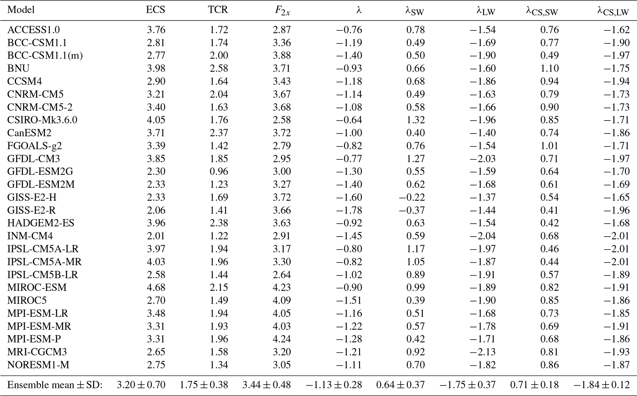
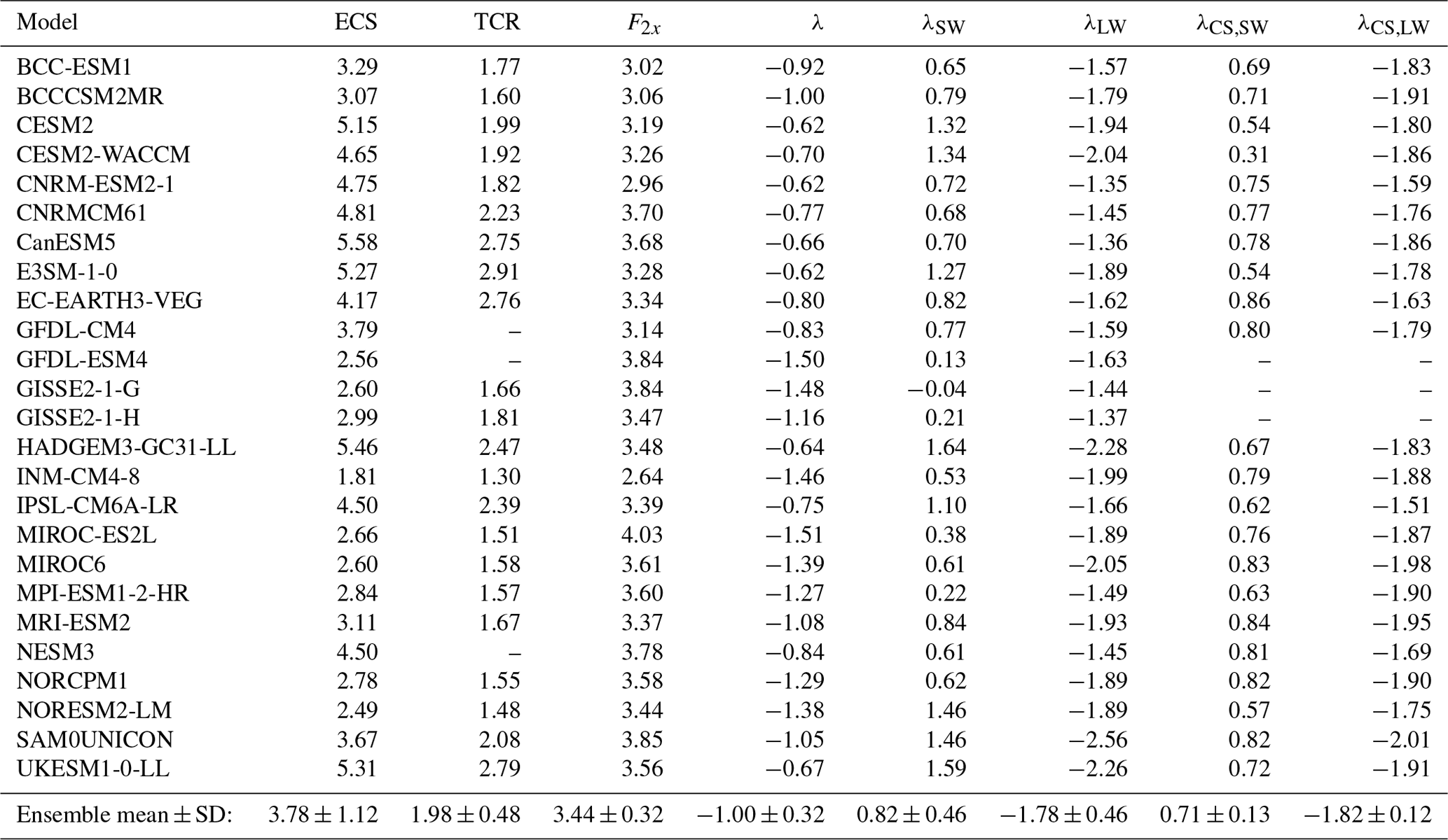
The CMIP5 ensemble analyzed in this work includes 27 models, and the CMIP6 ensemble includes the 25 members available at the time of writing. The first realization for each model (r1i1p1 for CMIP5 and r1i1p1f1 for CMIP6) was used, and all climate model output was downloaded from the Earth System Federation Grid (ESGF) nodes. All models are listed in Tables 1 and 2 with their ECS, TCR, and feedback parameter values.

2.1 Estimation of model climate sensitivities and feedbacks

The ECS for each model was calculated from the CMIP abrupt4xCO2 simulation, in which the CO₂ concentration is abruptly quadrupled at the beginning of the 150-year simulation and then held constant (Eyring et al., 2016). Since some models exhibit control state drift, accurate estimates of ECS and TCR require correcting for this, which we do here by assuming the underlying drift is approximately linear in time over the 150 years. The time slice of the pre-industrial control simulation (piControl), corresponding to the 150-year abrupt4xCO2 simulation is first chosen, beginning at the simulation year at which abrupt4xCO2 branched off of piControl. One must be cognizant that this information is not always reliable, so in a few cases the correction may not be accurate. A linear regression is then performed on the global annual mean piControl surface temperature or TOA radiative flux values to remove annual fluctuations, which is then used as the new piControl. The regression values are then subtracted from the global annual mean radiative fluxes and surface temperatures from abrupt4xCO2 to obtain the radiative flux and surface temperature anomalies. These resulting anomalies are linearly regressed against each other, following the Gregory method (Gregory et al., 2004), to obtain the ECS value as one-half of the x-intercept, the total climate feedback parameter λ as the slope of the regression, and the forcing as one-half of the y-intercept. This method does include what is often referred to as fast adjustments, insofar as they happen in much less than a year. The thus estimated forcing is, however, biased slightly low due to curvature of imbalance versus temperature found in several models. The ECS and feedback parameter do not change significantly if the global average, time average of the piControl is subtracted from abrupt4xCO2 instead of a linear regression; however, it should be noted that differences in methodology can contribute some uncertainty to the ECS magnitude (Boucher et al., submitted). Shortwave (SW) and longwave (LW) feedback parameters are calculated in a similar manner but using the TOA SW radiative flux anomalies or LW radiative flux anomalies, respectively, instead of the total flux.

TCR is calculated from the 1pctCO2 CMIP simulation (Eyring et al., 2016), in which CO₂ is gradually increased at a rate of 1 % per year. The corresponding time slice of piControl is first removed in the same manner as for ECS, to obtain the global annual mean 1pctCO2 surface temperature anomalies. TCR is then calculated as the mean surface temperature anomaly in a 20-year period centered on year 70 of the simulation; the year at which the CO₂ concentration is doubled.

2.2 Estimation of model and observational historical warming

Historical warming amounts were computed for each model. The early and late periods are defined as 1900–1969 (pre-1970s warming) and 1970–2005 (post-1970s warming), respectively, with years corresponding to the Santa María, Mt. Agung, El Chichón, and Pinatubo volcanic eruptions (1902–1904, 1963–1964, 1982–1984, and 1990–1993, respectively) excluded to limit the influence of natural volcanic aerosol forcing. Pre-1970s warming is strongly influenced by the uncertain aerosol cooling that offset some of the greenhouse gas warming (Stevens, 2015), whereas post-1970s warming is dominated by greenhouse gas warming, while aerosol cooling only changed slightly and so is expressive of TCR and ECS (Jiménez-de-la Cuesta and Mauritsen, 2019). The warming within each period is defined as the difference in the mean surface temperature between 1994–2005 and 1970–1989 for the late period and between 1900–1939 and 1940–1969 for the early period.

Model historical warmings are compared to the same periods from the Cowtan and Way (2014) version 2.0 surface temperature reconstruction for years 1850 to present. In this reconstruction the land surface temperatures and sea surface temperatures (SSTs) are based on the HadCRUT version 4.2.0 and UAH version 5.6 global surface temperature datasets. Missing data are infilled by kriging. Data coverage uncertainty and ensemble uncertainty, or uncertainty arising from the choice of parameter values used to create the reconstruction, are included in the data set. Uncertainty from natural variability within each warming period is computed based on the 100-member Max Planck Institut MPI-ESM1.1 model Grand Ensemble of historical climate change simulations (Maher et al., 2019), which is larger than the reconstruction uncertainties. Thus the total warming uncertainty is taken as the observational uncertainty (the coverage uncertainty and reconstruction parameter uncertainty) plus uncertainty due to natural climate variability estimated from the MPI Grand Ensemble, summed in quadrature.

3 Comparison of the model ensembles

In this section we will first inspect the global ECS and feedback parameters in the two CMIP ensembles, and then we ask whether the shift could have happened by chance.

3.1 Shifts in climate sensitivity and global feedbacks between CMIP5 and CMIP6

Figure 1 displays the distributions of ECS for CMIP5 and CMIP6, with the mean value and standard deviation (SD) for each ensemble also displayed. The ensemble mean ECS increased from 3.2 K (range of 2.0–4.7 K) for CMIP5 to 3.7 K (1.8–5.5 K) for CMIP6, an increase of 0.5 K or 17%. Moreover, the CMIP6 distribution is shifted towards higher ECS, with a secondary peak at approximately 5 K. About 11% of CMIP5 models have an ECS greater than 4 K, compared to 40% of CMIP6 models. Only one CMIP6 model, INM-CM4-8, exhibits a smaller ECS (1.81 K) than is found in any model in CMIP5.

The average radiative forcing from CO₂, as estimated using the Gregory method (Gregory et al., 2004), does not change substantially between the CMIP ensembles, whereas the range narrows slightly (Fig. 2 and Tables 1 and 2). The total feedback parameter λ, however, does exhibit an increase in ensemble mean, from −1.13 ${\mathrm{Wm}}^{-\mathrm{2}}{\mathrm{K}}^{-\mathrm{1}}$ (± 0.28) to −1.02 ${\mathrm{Wm}}^{-\mathrm{2}}{\mathrm{K}}^{-\mathrm{1}}$ (± 0.32). This shift towards less negative values is also discernible in Fig. 2, particularly for models with ECS on the high end. Therefore, the decrease in λ magnitudes, which alone determines most of the variation in ECS, is the main driver behind the shift toward higher ECS between the CMIP ensembles.

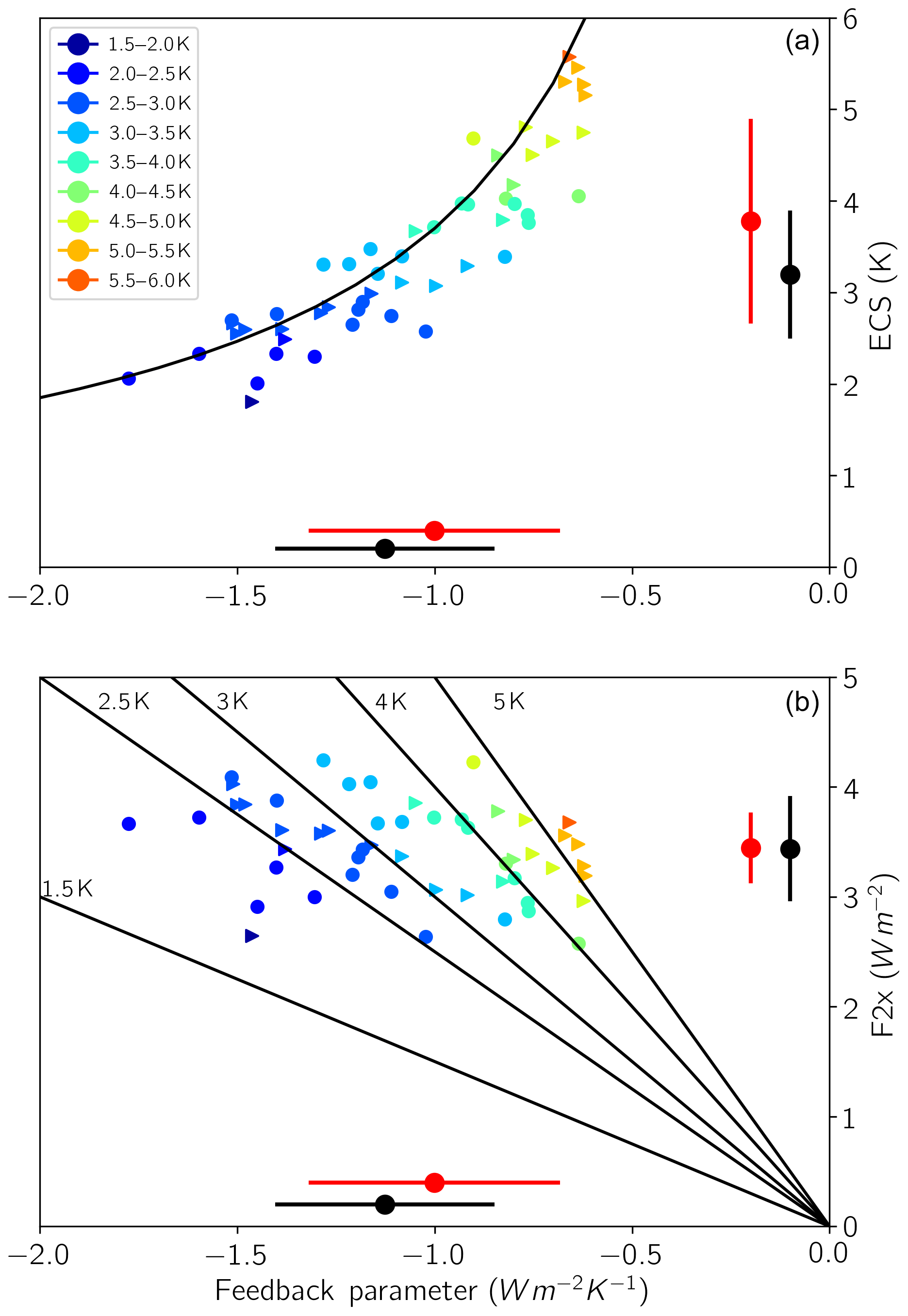
Figure 2 ECS versus total net feedback parameter. The black curve represents the expected ECS value based on a forcing of 3.7 Wm⁻² over the range of feedbacks plotted (a) and effective forcing versus total net feedback parameter. The black lines represent the expected forcing–feedback relationship based on the ECS value given in the label of each line (b). Circles represent CMIP5 models, and right-facing triangles represent CMIP6 models. Mean value and SD for each parameter for the CMIP5 and CMIP6 ensembles displayed in black and red, respectively, on the appropriate axis in each plot. Plot symbols are colored by ECS values as shown in the legend.

Table 1 List of CMIP5 models and model climate parameters.

Table 2 List of CMIP6 models and model climate parameters.

3.2 Could we obtain the CMIP6 ensemble mean ECS by chance?

The results presented in Sect. 3.1 demonstrated a clear shift in ECS from CMIP5 to CMIP6 but did not establish if that shift was statistically significant. The recently published Zelinka et al. (2020) found their increase in ensemble-mean ECS to be just short of statistical significance (95% confidence level or p<0.05) using a Welch's t test for equal means; this t test does not assume equal variance in the samples being compared. However, for the subset of CMIP5 and CMIP6 models examined in this work, also using a Welch's t test, we obtain a statistically significant shift. This may seem to be inconsistent at first glance, but it should be noted that Zelinka et al. (2020) included some models which we did not and vice versa, which may influence the results of t tests.

However, a potential complication exists when applying such standard methods to compare mean ECS: statistical tests for independence of means such as t tests usually rely on an assumption of a Gaussian or approximately Gaussian underlying distribution and may not be appropriate for samples with skewed distributions, such as ECS (Roe and Baker, 2007).

Instead, one might view such generational ensembles as small random samples taken from some generic modeling activities that are subject to noise. In this view, how likely is it that we obtain the CMIP6 ensemble mean ECS increase simply by chance? In other words, do the high CMIP6 climate sensitivities represent a statistically significant shift in an envisioned underlying probability distribution based on modeling, or are they encapsulated by the uncertainty of climate modeling? We address the question of statistical significance by assuming the underlying ECS distribution is well described by Eq. (1).

First, one must understand that the mean of the resulting ECS distribution is generally larger than the median, caused by the positive skewness of the distribution (Roe and Baker, 2007); it should be noted that using the mean λ and mean F_2x in Eq. (1) therefore represents the median rather than the mean ECS as the centroid of the underlying distribution. We assume a Gaussian distribution for λ and F_2x, then compute the ECS distribution with Eq. (1) and determine the median ECS values that correspond to the CMIP5 and CMIP6 means; the probability of obtaining either CMIP mean from the resulting distribution can then be assessed. To show how the mean and median of the underlying ECS distribution differ, we Monte Carlo sample feedback parameters from Gaussian distributions with a SD equal to the average of the CMIP5 and CMIP6 ensemble SDs (0.29 ${\mathrm{Wm}}^{-\mathrm{2}}{\mathrm{K}}^{-\mathrm{1}}$; see Tables 1 and 2) and forcing centered on 3.7 Wm⁻² with a SD of 10 %. This is the current best estimate (Etminan et al., 2016), and choosing a different value has no appreciable effect on our results, as forcing is in the numerator. A range of median ECS values, including probable and improbable values from between 0.1 and approximately 6 K (corresponding to mean feedback parameters of −37 to −0.63 ${\mathrm{Wm}}^{-\mathrm{2}}{\mathrm{K}}^{-\mathrm{1}}$ when forcing is set to −3.7 Wm⁻²), were assessed, all with the SD set to 0.29 ${\mathrm{Wm}}^{-\mathrm{2}}{\mathrm{K}}^{-\mathrm{1}}$. Negative ECS and values exceeding 10 000 K are omitted. For each value of median ECS we can then evaluate the resulting mean, which is quite close for lower values of median ECS but diverges for higher sensitivities (Fig. 3a). For the CMIP5 mean of 3.2 K, the corresponding median is 3.0 K, and for the CMIP6 mean of 3.7 K the median is 3.4 K.

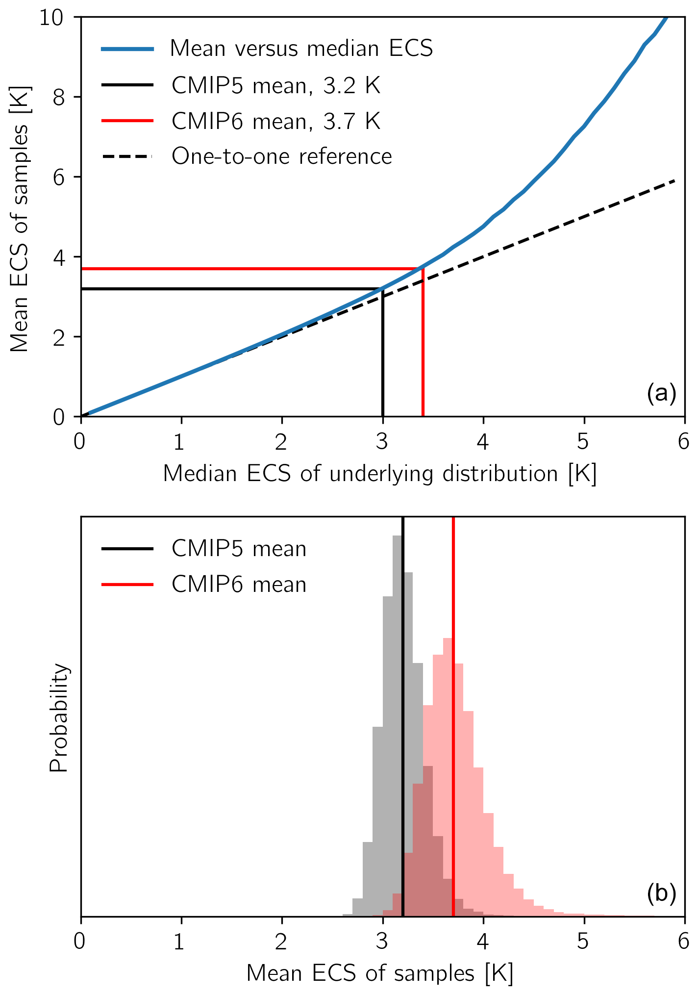
Figure 3 Random sampling of ECS from Gaussian distributions of λ and F_2x. Panel (a) shows the relationship between the median and mean of ECS, arising from the inverse relationship between ECS and λ. Panel (b) shows distributions of mean ECS from random 25-member ensembles centered at the means of CMIP5 and CMIP6.

Using these medians we next address the question of whether CMIP6 could be obtained simply by chance. To do so, we first assume the underlying median ECS is 3.0 K and make 100 000 random ensembles, each with 25 models (the size of the CMIP6 ensemble studied here). The resulting distribution of mean ECS values of the random ensembles is shown in Fig. 3. It turns out that less than 2 % of the samples exceed 3.7 K, which is the mean of CMIP6. Likewise, if we assume the underlying median is 3.4 K, centered at CMIP6, then less than 2 % of the samples have a mean less than 3.2 K, which is the mean of CMIP5. Thus, the shift in ensemble mean ECS between CMIP5 and CMIP6 is extremely unlikely to have been caused simply by chance.

4 Decomposition into longwave and shortwave feedbacks

Having established that there is a systematic shift in feedback underlying the increase in ensemble mean ECS from CMIP5 to CMIP6, we next divide the feedback into longwave, shortwave, all-sky, and clear-sky components and inspect the zonal mean distribution in order to seek the possible underlying causes.

4.1 Global-mean all-sky and clear-sky feedbacks

Decomposition of the total feedback parameter into the all-sky shortwave (SW; λ_SW) and longwave (LW; λ_LW) components and examination of the clear-sky (CS) SW and LW feedbacks (λ_CS,SW; λ_CS,LW), elucidates which classes of feedbacks drive the increase in ECS. As shown in Fig. 4a, a systematic shift toward more positive λ_SW has occurred on average for the CMIP6 ensemble relative to CMIP5: the mean λ_SW increased from 0.64 to 0.73 ${\mathrm{Wm}}^{-\mathrm{2}}{\mathrm{K}}^{-\mathrm{1}}$, whereas the mean λ_LW remained almost unchanged (mean of −1.74 and −1.78 ${\mathrm{Wm}}^{-\mathrm{2}}{\mathrm{K}}^{-\mathrm{1}}$, respectively). However, much spread in the SW and LW feedbacks exists within both ensembles as indicated by the large SDs.

Figure 4 All-sky λ_LW versus λ_SW for the CMIP5 and CMIP6 ensemble (a) and clear-sky λ_CS,LW versus λ_CS,SW for CMIP5 and CMIP6 (b). CMIP5 is shown as circles, and CMIP6 is shown as right-facing triangles. Mean CMIP5 feedbacks and SDs are shown as black circle and lines, and mean CMIP6 and SDs are shown as dark gray triangle and lines in each plot. Lines of constant ECS based on forcing of 3.7 Wm⁻² are given in light gray. Plot symbols colored by ECS values are as shown in the legend.

The shortwave feedback parameters are strongly associated with the total feedback parameter for both model ensembles, with a correlation coefficient of 0.83 (p value less than 0.001) for CMIP5 and 0.56 (p value of 0.004) for CMIP6, whereas the longwave feedbacks exhibited small, statistically nonsignificant correlations with the total feedback parameter (−0.21 and 0.11 for CMIP5 and CMIP6, respectively). The longwave thus exhibits no consistent or systematic shift with ECS, whereas these results suggest that λ_SW is the main cause of both the variations and the shift in λ and thus of ECS. These feedbacks suggest that much of the spread is caused by cloud parameterizations and that cloud feedbacks play an important role in the shift to higher ECS in CMIP6.

In contrast, no systematic shifts are evident in the clear-sky feedback parameters (λ_CS,SW or λ_CS,LW) between the CMIP eras (Fig. 4), and again much spread among models is evident in both ensembles. However, the spread in CMIP6 λ_CS,SW is smaller than that for CMIP5, with a SD of 0.13 compared to 0.18 ${\mathrm{Wm}}^{-\mathrm{2}}{\mathrm{K}}^{-\mathrm{1}}$, indicating a greater convergence of the CMIP6 λ_CS,SW values, while the SDs for the clear-sky longwave feedbacks are of similar magnitude (0.12 ${\mathrm{Wm}}^{-\mathrm{2}}{\mathrm{K}}^{-\mathrm{1}}$). This is in contrast to the all-sky feedbacks, where the SDs were larger for both SW and LW for CMIP6. Lastly, the clear-sky feedbacks in Fig. 4b do not exhibit a statistically significant slope for both ensembles despite the spread among models, whereas the all-sky feedbacks (Fig. 4a) exhibited statistically significant, negative slopes (−0.37 and −0.47 for CMIP5 and CMIP6, respectively); the dominant direction of the spread has changed between all-sky and clear-sky. Thus, another feedback besides cloud feedback may be causing the spread, such as the surface albedo feedback; it is also notable that the spread in λ_CS,SW decreased between CMIP5 and CMIP6, suggesting a shift in the underlying albedo feedback between ensembles.

4.2 Zonal-mean feedbacks

The all-sky and clear-sky feedback parameters are decomposed into zonal-mean feedback parameters, to further investigate the causes of the shifts in the shortwave feedbacks and which regions may be the main drivers. The zonal mean feedbacks are calculated similarly to the global annual mean feedbacks, with the exception that the global annual mean surface temperature anomalies are regressed instead against zonal annual mean TOA imbalances. The radiation fluxes are first divided into 10^∘ latitude bins based on each model's grid, centered between 85^∘ S and 85^∘ N, and then the Gregory method is applied to compute the zonal-mean all-sky and clear-sky feedbacks. These feedbacks are displayed in Fig. 5 as a function of latitude for all-sky and Fig. 6 for clear-sky.

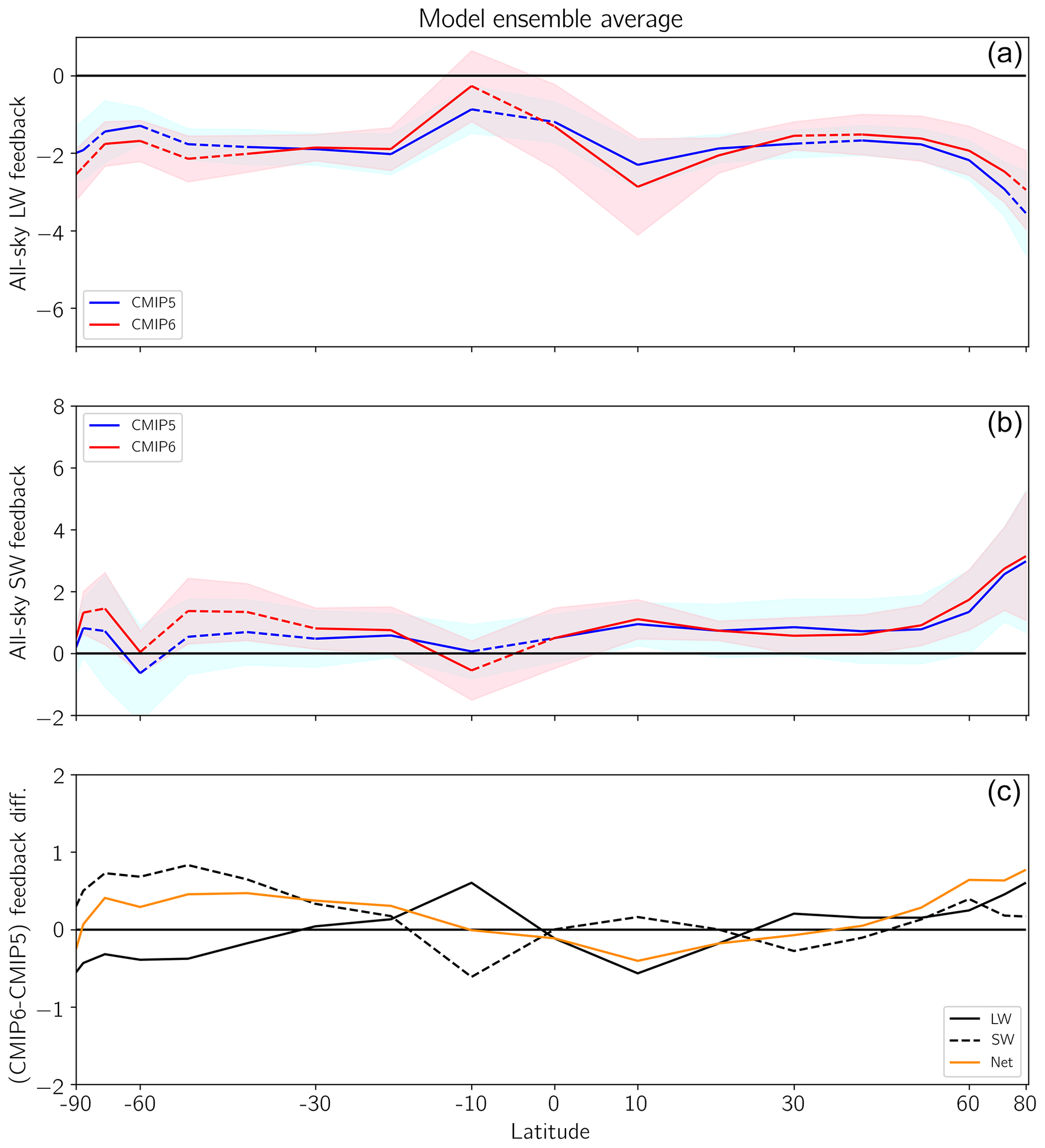
Figure 5 All-sky zonal average λ_LW (a) and λ_SW (b) for the CMIP5 ensemble average (blue) and CMIP6 ensemble (red). Dashed blue and red lines indicate regions where the difference in mean feedback is statistically significant (p<0.05). Light blue and red shading represent SD of each ensemble. Panel (c) displays the difference between the CMIP6 and CMIP5 ensemble average SW, LW, and net feedbacks as a function of latitude.

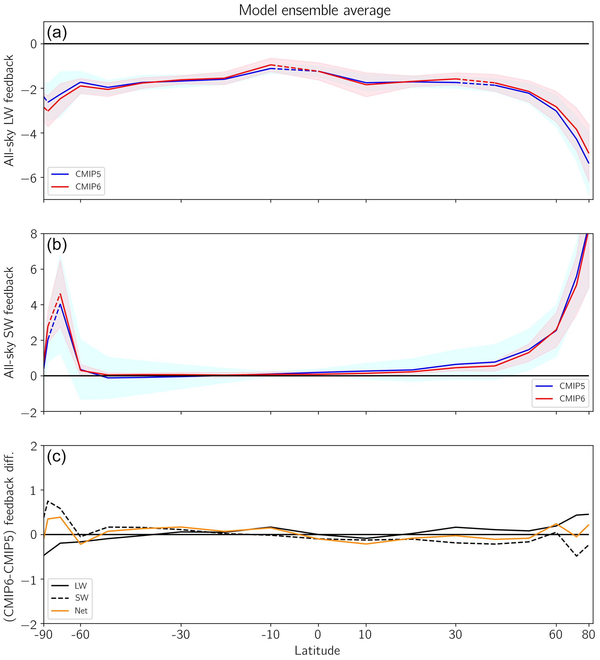
Figure 6 Clear-sky zonal average λ_CS,LW (a) and λ_CS,SW  (b) for the CMIP5 ensemble average (blue) and CMIP6 ensemble (red). Dashed blue and red lines in (a) and (b) indicate regions where difference in mean feedback is statistically significant (p<0.05). Light blue and red shading represent SD of each ensemble. Panel (c) displays the difference between the CMIP6 and CMIP5 ensemble average SW, LW, and net feedbacks.

Large differences in all-sky feedbacks between CMIP eras tend to occur in the tropics and towards the poles. In particular, a broad swath of change is seen for the Southern Hemisphere midlatitude and polar regions; the largest shortwave feedback differences are found in these regions, where the CMIP6 zonal shortwave feedbacks have substantially increased (Fig. 5). Statistically significant (p<0.05) differences in ensemble-mean zonal shortwave feedback, however, occur solely within the Southern Hemisphere, within the deep southern tropics (0–10^∘ S), the extratropics (30–60^∘ S), and in the polar region between 70–80^∘ S. Though smaller in magnitude, clear-sky zonal shortwave feedback also shows substantial increases between CMIP5 and CMIP6 poleward of 60^∘ S in the Southern Ocean (Fig. 6). The broad increases from CMIP5 to CMIP6 in all-sky λ_SW across much of the Southern Hemisphere extratropics, coupled with changes in clear-sky feedback only within the southern polar regions, further indicate that cloud feedbacks have changed between CMIP eras. It is also notable that the variability among models within the CMIP6 ensemble has decreased relative to CMIP5 in the shortwave for both all-sky and clear-sky, as indicated by the smaller SD bounds on the ensemble averages in Figs. 5 and 6; the CMIP6 models display greater agreement on the magnitude and sign of the zonal shortwave feedbacks, though whether CMIP6 has become more realistic cannot be determined here.

The largest and only statistically significant clear-sky shortwave feedback changes occur over the Southern Ocean latitudes (Fig. 6b and c), where a shift towards more positive clear-sky shortwave feedback is found. This is suggestive of increases in the sea-ice-induced surface albedo feedback in CMIP6, likely due to increased abundance of sea ice near the Antarctic in the underlying piControl climatology in CMIP6 relative to CMIP5 (Fig. 7). In fact, the only statistically significant change in piControl sea ice coverage is found in the Southern Ocean. Perhaps as a result of this larger base-state abundance, the decrease in sea ice coverage in the Antarctic in the abrupt4xCO2 simulation is also greater for CMIP6 than CMIP5 (Fig. 7). This reduction in sea ice abundance in abrupt4xCO2 shown in Fig. 7, defined as the difference between the mean of the last 30 years of abrupt4xCO2 and the mean over the piControl climatology, is statistically significantly (p<0.05) correlated with ECS for the 70–80^∘ S and 60–70^∘ S latitude bands for the CMIP6 ensemble (correlation coefficient of −0.8 and −0.69, respectively); no statistically significant correlations were found between sea ice reductions in abrupt4xCO2 and ECS for CMIP5 within the Southern Hemisphere. Greater decreases in Antarctic sea ice in abrupt4xCO2 are thus strongly associated with larger ECS, likely through strengthening of the sea ice albedo as indicated by the shift towards more positive clear-sky shortwave feedbacks in this region. Further, regional maps of the difference in clear-sky shortwave feedbacks (Fig. 8) and sea ice between CMIP5 and CMIP6 (Fig. 9) demonstrate that the increased base-state sea ice abundance in piControl, greater reductions in sea ice in abrupt4xCO2, and more positive clear-sky shortwave feedbacks track each other over much of the Southern Ocean; for example, larger clear-sky feedbacks in the region of the Bellingshausen and Amundsen seas are associated with larger base-state sea ice and larger sea ice reductions with warming. These features are found in most regions of the Southern Hemisphere, with the exception of a region off eastern Antarctica displaying smaller clear-sky zonal feedbacks in CMIP6 than CMIP5, suggesting that changes across most of the Southern Ocean are responsible for the increased shortwave feedbacks.

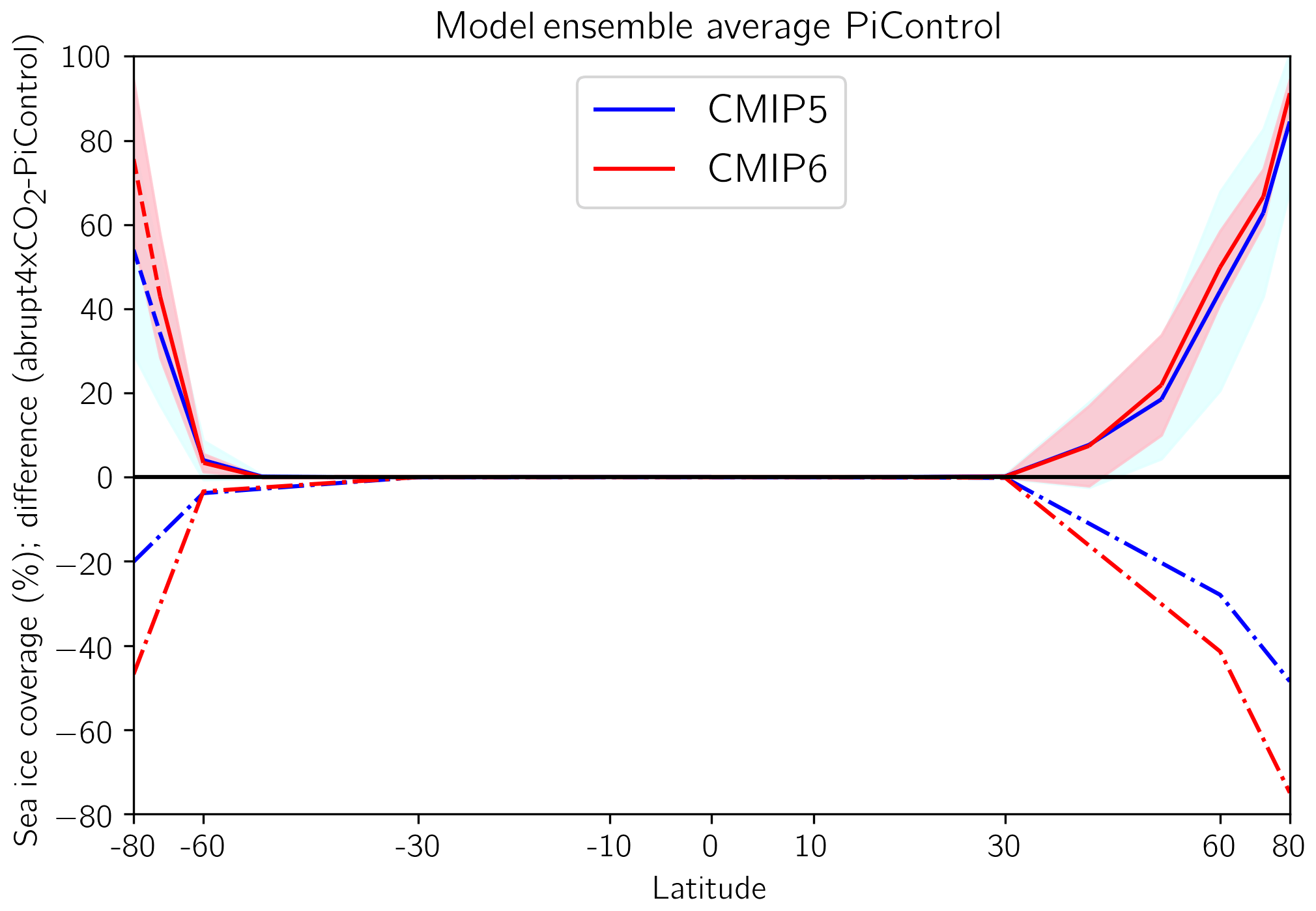
Figure 7 Zonal average sea ice coverage from piControl for the CMIP5 ensemble (blue) and CMIP6 ensemble (red) shown as solid red and blue lines; dashed lines in these curves indicate regions where difference in mean sea ice coverage is statistically significant (p<0.05). Light blue and red shading around the solid lines represent SD of each ensemble. Dashed-dotted lines represent the average difference in sea ice coverage between the zonal average piControl simulation (over the 150 years corresponding to abrupt4xCO2) and the mean of the last 30 years of the abrupt4xCO2 simulation.

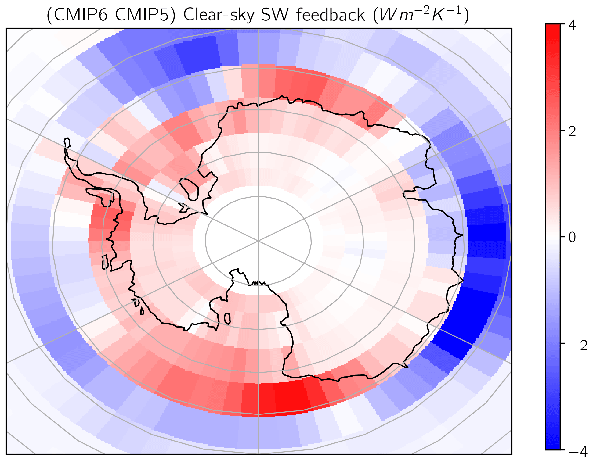
Figure 8 Map of the difference in clear-sky zonal feedbacks for the Antarctic region between CMIP6 and CMIP5. Red colors indicate that the CMIP6 feedback is larger than CMIP5, and blue indicates that CMIP6 is smaller than CMIP5. Averaged on a 5^∘ by 5^∘ grid.

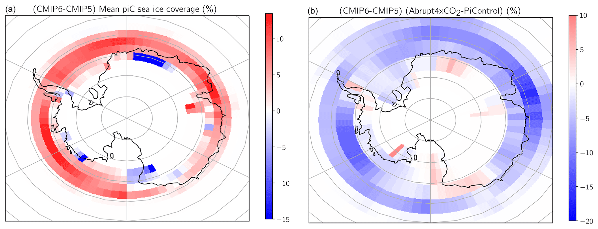
Figure 9 (a) Map of the difference in mean piControl sea ice abundance climatology between CMIP6 and CMIP5 in the Antarctic and (b) of the difference between CMIP6 and CMIP5 in the reduction of sea ice abundance in abrupt4xCO2. Reduction in sea ice for each CMIP ensemble calculated as difference in sea ice coverage between the average piControl simulation (over the 150 years corresponding to abrupt4xCO2) and the mean of the last 30 years of the abrupt4xCO2 simulation. Averaged on a 5^∘ by 5^∘ grid.

Larger decreases in sea ice coverage for abrupt4xCO2 are also seen in the Arctic but are accompanied by a much smaller (and statistically insignificant) change in shortwave feedback relative to the Antarctic; the underlying piControl sea ice coverage did not significantly increase between CMIP5 and CMIP6 in the Arctic, leading to a lesser impact on the sea ice albedo feedback. Furthermore, in contrast to the Antarctic, the difference in net feedback in the Arctic is smaller than for the Antarctic, and the change in the clear-sky shortwave feedback in Northern Hemisphere midlatitudes is negative (albeit statistically insignificant; Fig. 6). Perhaps as a result there is less intense Arctic amplification exhibited by CMIP6 relative to CMIP5 (Fig. 10). Surface temperature increases in the Arctic still exceed warming elsewhere in the CMIP6 ensemble, but of a somewhat smaller magnitude than CMIP5, likely due to a relatively lessened impact of sea ice albedo on the feedback parameter.

Figure 10 Zonal average surface temperature anomaly from abrupt4xCO2 relative to piControl for the CMIP5 ensemble average (blue) and CMIP6 ensemble (red). Light blue and red shading represent the SD of each ensemble. Dashed blue and red lines indicate regions where the difference in mean feedback is statistically significant (p<0.05).

We speculate that much of this behavior can be explained by an increased focus on the representation of mixed-phase clouds by the models' microphysics parameterizations. Recent studies have shown that the strength of the negative cloud optical depth feedback is strongly dependent on the relative partitioning of ice- and liquid-phase cloud condensate in the control state (Tan et al., 2016). By increasing the amount of liquid in supercooled clouds the negative optical depth feedback is weakened and hence ECS increases. In addition, since liquid clouds are generally more reflective than ice clouds, the long-standing Southern Ocean warm bias may have been reduced through these efforts, thereby resulting in more abundant sea ice. These effects could, together, explain the nontrivial increase in ECS in the CMIP6 ensemble over CMIP5.

Our feedback analysis results are broadly in agreement with those of Zelinka et al. (2020). The global and zonal all-sky shortwave feedbacks examined here clearly point to clouds as the main driver behind the shift towards more positive total feedback, which in turn drove the shift towards higher ECS. Zelinka et al. (2020) also found the increase in ECS to be due to less negative total feedback, driven by stronger positive low cloud shortwave feedbacks. Using radiative kernels and the approximate partial radiative perturbation technique to further analyze the cloud feedbacks, they determined that the shortwave low cloud amount and optical depth (essentially what is referred to in Zelinka et al., 2020, as the scattering feedback) feedbacks shifted towards more positive values in CMIP6, particularly in the extratropics; this shift ultimately drove the total feedback parameter towards less negative values. As in this work, the analysis of Zelinka et al. (2020) pointed towards changes in model representation of cloud processes in CMIP6 relative to CMIP5. Further, statistically significant increases in ensemble zonal mean low cloud amount feedback were found in the Southern Hemisphere extratropics, consistent with our statistically significant southern extratropical differences in all-sky zonal feedbacks (though these include more than just cloud feedbacks). Notably, Zelinka et al. (2020) found a decrease in the spread of the albedo feedback for CMIP6, consistent with the reduction in variability we found for the clear-sky shortwave feedback, and Fig. S7 in their supplemental material indicates that strengthened extratropical albedo feedback may be an important secondary driver of the increase in ECS for many CMIP6 models. This is again consistent with our results for the zonal shortwave clear-sky feedback, which also demonstrate a decreased spread in clear-sky shortwave feedbacks for CMIP6. Our zonal feedback analysis suggests that the increased albedo feedback is found primarily in the Southern Ocean and is linked to increased sea ice coverage in this region in the CMIP6 piControl climatology. Increased base-state sea ice coverage likely caused greater reductions in sea ice in the abrupt4xCO2 simulations, which are associated with strengthened zonal clear-sky shortwave feedbacks (as sea ice albedo feedback) in the Southern Ocean and larger ECS. Model changes in representation of clouds and sea ice are thus the likely culprits causing the change in sea ice climatology, though the details of such changes and their effects may vary among models and warrant further investigation.

5 Transient climate response, historical warming, and aerosol cooling

The instrumental record warming is the prima facie test of climate models: if models are not able to reproduce the history of warming then they do not represent a credible hypothesis of how the climate system works. However, the warming in a model is a result of both climate change feedbacks, radiative forcing, deep-ocean heat uptake, and pattern effects, and therefore modellers can trade off these factors to obtain an overall warming in line with observations (Kiehl, 2007). Some modeling centers use this explicitly to tune their models (Hourdin et al., 2017; Mauritsen et al., 2019), whereas others state they do not do this (Schmidt et al., 2017). In either case, representing historical warming is a necessary but insufficient validation of a climate model.

A central metric that incorporates several of the factors relevant for historical warming is the transient climate response (TCR). TCR is computed from an idealized simulation with a gradual 1% per year CO₂ increase as the warming around the time of doubling. Just as for ECS, TCR also has increased in CMIP6 to a mean of 1.98 K (range 1.30–2.91 K) compared to the CMIP5 mean of 1.75 K (0.96–2.58 K), as seen in Fig. 11. One can obtain an approximate estimate of TCR in terms of physical bulk properties of the climate system (Jiménez-de-la Cuesta and Mauritsen, 2019):

$$\begin{array}{}\text{(2)}& \text{TCR}\approx {\displaystyle \frac{-F_{\mathrm{2}x}}{\mathit{\lambda }-\mathit{ϵ}\mathit{\gamma }}},\end{array}$$

where the product ϵγ is equal to 0.93 ${\mathrm{Wm}}^{-\mathrm{2}}{\mathrm{K}}^{-\mathrm{1}}$, with an uncertainty range of 0.54–1.32 ${\mathrm{Wm}}^{-\mathrm{2}}{\mathrm{K}}^{-\mathrm{1}}$ in CMIP5 (Geoffroy et al., 2013); ϵ is the deep-ocean heat uptake efficacy representative of forced temporary pattern effects; and γ is the deep-ocean heat uptake coefficient. The product ϵγ controls the relationship between TCR and ECS. Models in CMIP6 follow the predicted behavior of Eq. (2) using CMIP5 parameters surprisingly well (Fig. 11). However, the mean of ϵγ increased to 0.98 ${\mathrm{Wm}}^{-\mathrm{2}}{\mathrm{K}}^{-\mathrm{1}}$, while the uncertainty range decreased (0.73–1.23 ${\mathrm{Wm}}^{-\mathrm{2}}{\mathrm{K}}^{-\mathrm{1}}$) based on the CMIP6 ensemble examined here relative to CMIP5. Though not a statistically significant difference between the two means, several CMIP6 models with high TCR and ECS now fall outside the upper uncertainty bound for expected TCR when using ϵγ based on CMIP6 (Fig. 11). These four high-TCR CMIP6 models are associated with much smaller values for ϵγ (0.54–0.69 ${\mathrm{Wm}}^{-\mathrm{2}}{\mathrm{K}}^{-\mathrm{1}}$) and the total feedback parameter (between −0.80 and −0.62 ${\mathrm{Wm}}^{-\mathrm{2}}{\mathrm{K}}^{-\mathrm{1}}$), though it is left to future work to disentangle the shifts in specific phenomena, such as pattern effects, that contribute to this.

Figure 11 TCR versus ECS for the CMIP5 ensemble (black circles) and CMIP6 ensemble (right-facing red triangles). Expected values based on forcing of 3.7 Wm⁻² and a value of $\mathit{ϵ}\mathit{\gamma }=\mathrm{0.93}{\mathrm{Wm}}^{-\mathrm{2}}{\mathrm{K}}^{-\mathrm{1}}$ are shown by the black curve, and uncertainty of the ϵγ value is shown as gray bounding lines. Dashed black and gray curves represent the same expected values but are based on a value of $\mathit{ϵ}\mathit{\gamma }=\mathrm{0.98}{\mathrm{Wm}}^{-\mathrm{2}}{\mathrm{K}}^{-\mathrm{1}}$ computed from the CMIP6 ensemble. ECS and TCR mean values and SDs for the CMIP5 and CMIP6 ensembles are displayed in black and red, respectively.

Given that TCR is on average higher in CMIP6 one might naively expect stronger historical warming; however, this is not the case (Fig. 12). Whereas CMIP5 on average tracked the instrumental record quite well, warming slightly too much in the latter half of the 20th century, the CMIP6 models are systematically on average colder than observed starting around 1940 but nearly catch up with global warming in the beginning of the 21st century. Looking at individual model simulations (Fig. 13) reveals that the spread in overall centennial warming also increased in CMIP6 and furthermore that there is not a strong relationship with TCR.

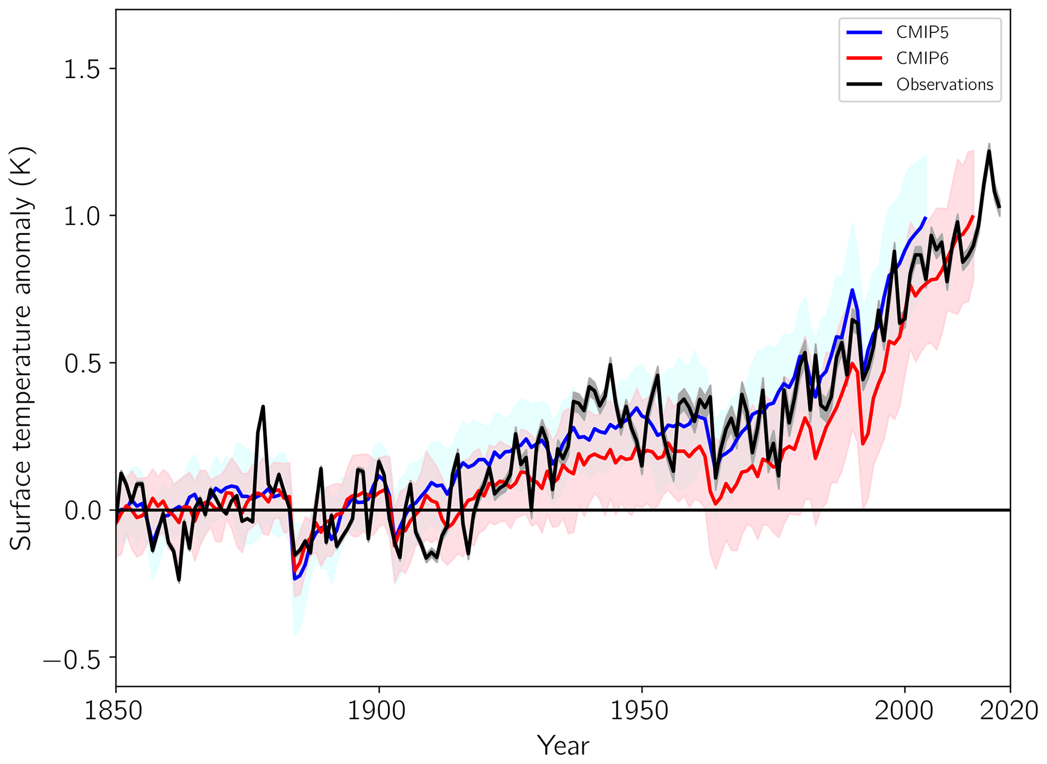
Figure 12 Ensemble mean historical surface warming in CMIP5 and CMIP6 compared with observations. Shading on the models is the ensemble SD. The baseline is 1850–1900.

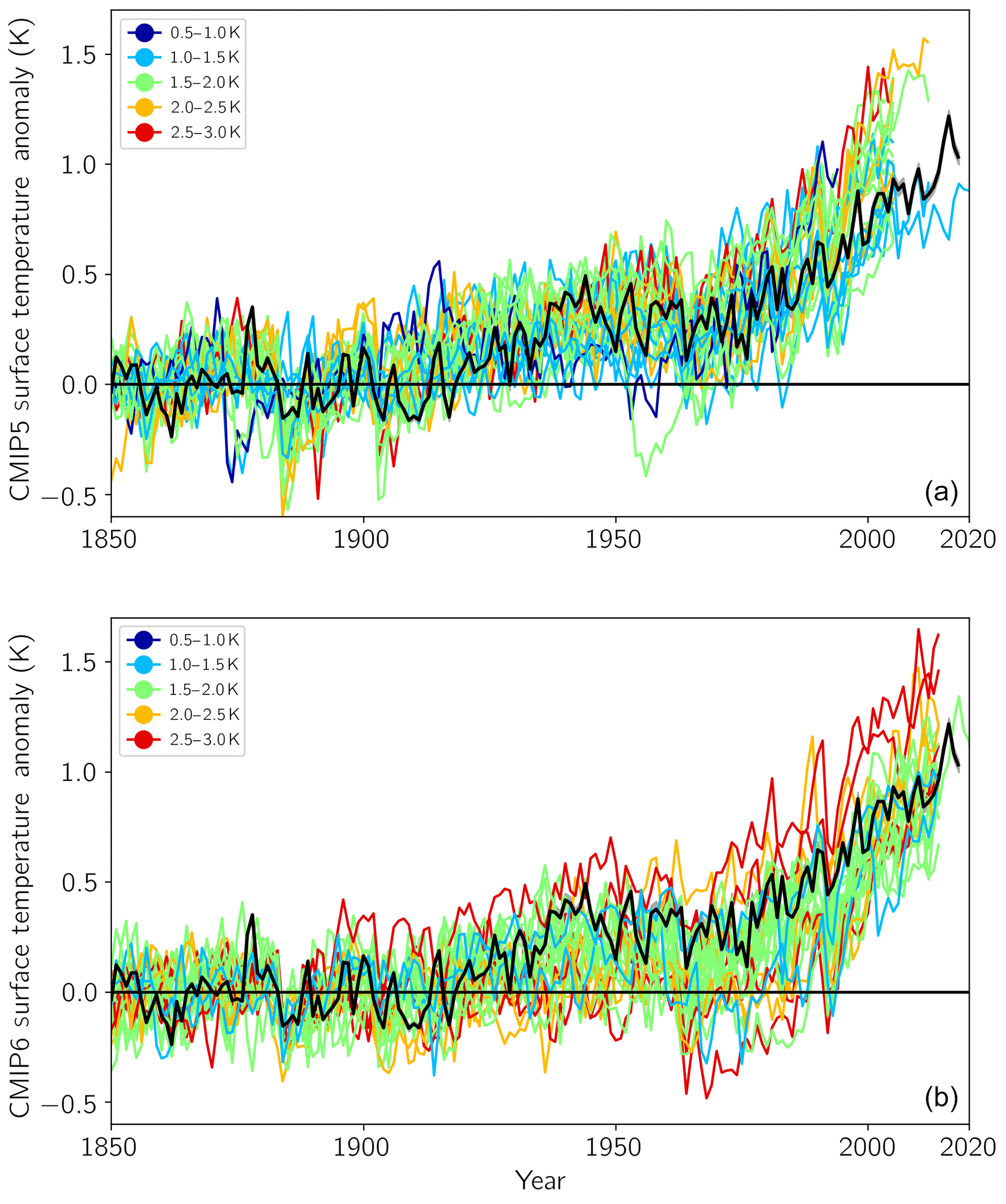
Figure 13 As in Fig. 12 but for individual model runs. Panel (a) shows CMIP5 models, and panel (b) shows CMIP6 models. Color coding is according to the respective models' TCR.

To demonstrate at this point that the most likely explanation for why CMIP6 on average warms less is because of stronger aerosol cooling we divide warming into the pre-1970s and post-1970s (Fig. 14). The rationale behind this division is that aerosol cooling, which has offset some of the greenhouse gas warming, increased rapidly with industrialization up until around 1970, when air quality regulations being implemented resulted in stabilized global aerosol cooling. Since the amount of anthropogenic aerosol cooling, in contrast to greenhouse gas warming, is highly uncertain (Bellouin et al., 2019) and varies among models, total forcing uncertainty in the pre-1970s period dominates the global temperature response (Stevens, 2015). In the post-1970s period, the greenhouse gas forcing change instead dominates and is less uncertain, such that the variations in TCR are more important (Jiménez-de-la Cuesta and Mauritsen, 2019).

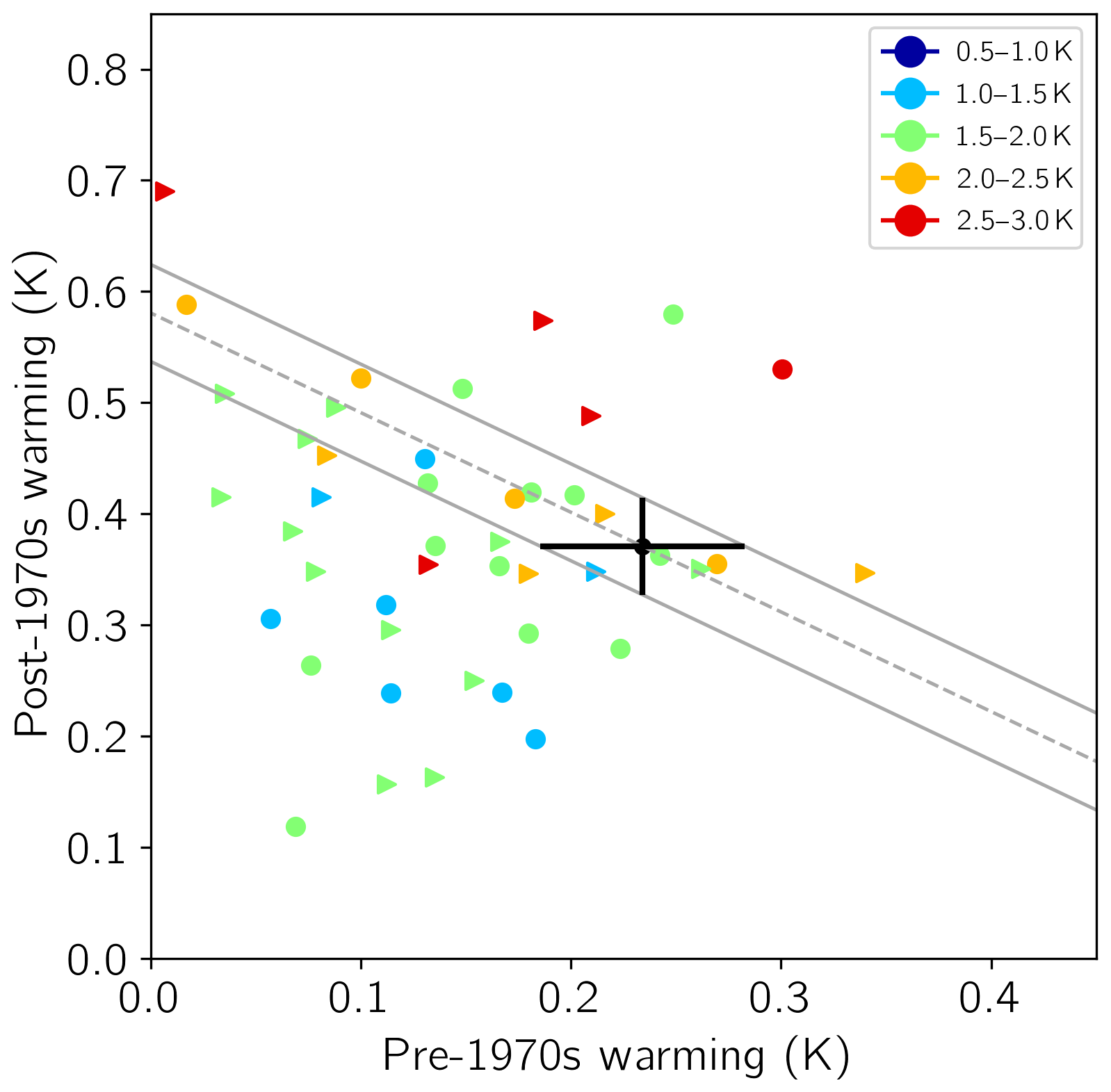
Figure 14 Post-1970s warming (surface temperature change between the 1970–1990 and 1994–2005 periods) versus pre-1970s warming (surface temperature change between the 1900–1939 and 1940–1969 periods), with plot symbols colored by TCR bins shown in the legend. Circles represent CMIP5 models, and right-facing triangles represent CMIP6 models. Observational pre- and post-1970s warming is plotted as a black circle with uncertainty as black lines. Solid gray lines represent the outer bounds of pre- and post-1970s warming, summing to total observed warming.

Interestingly, the majority of models from both ensembles underpredict the pre-1970s warming (Fig. 14), with a few CMIP6 models exhibiting close to no warming and several exhibiting less than 0.1 K of warming. This is a strong indication that many models apply too strong aerosol cooling and that this is more outspoken in CMIP6. About half the models, however, make up for this lack of warming by instead warming more than observed in the post-1970s period. As expected, there is no apparent relationship between pre-1970s warming and TCR, but a correlation exists with post-1970s warming, with higher TCR models exhibiting larger post-1970s warming. This is most apparent for models with TCR of 1.5–2.0 K (statistically significant correlation coefficient of 0.72 for CMIP6; CMIP5 correlation is not significant) and smaller or nonsignificant correlation for other TCR ranges. None of the models with TCR greater than 2.5 K provide a realistic post-1970s warming. Unfortunately, Radiative Forcing Model Intercomparison Project (RFMIP)-style simulations are available for CMIP6 but not for CMIP5, as these types of experiments are best suited for deciphering the causes of the exaggerated aerosol cooling.

6 Conclusions

We have compared the CMIP5 and CMIP6 model ensembles in terms of their climate sensitivities, feedback parameters, and historical warming evolution. The ECS and total feedback parameter values were computed with the Gregory method, and we found that both the ensemble mean ECS and the spread in ECS values has increased between CMIP5 (mean 3.2 K, spread 2.0–4.7 K) and CMIP6 (mean 3.7 K, spread 1.8–5.5 K).

We examined whether this shift in ECS between ensembles could have arisen simply by chance or whether it is a statistically significant change. This is a critical question because it speaks to whether such a shift in ECS is truly unexpected or not. We modeled distributions of forcing and feedbacks as random samples from Gaussian distributions centered at CMIP5 and determined that the probability of obtaining the CMIP6 ensemble mean ECS value was less than 2 %. Previous model ensemble mean ECS values are similar to those obtained for the CMIP5 ensemble, together suggesting that the CMIP6 ensemble mean ECS is indeed highly unusual.

This shift towards higher ECS for the CMIP6 ensemble is primarily driven by increases in the shortwave feedback parameter for some models within the ensemble. The mean total feedback parameter increased from −1.13 ${\mathrm{Wm}}^{-\mathrm{2}}{\mathrm{K}}^{-\mathrm{1}}$ for CMIP5 to −1.02 ${\mathrm{Wm}}^{-\mathrm{2}}{\mathrm{K}}^{-\mathrm{1}}$ for CMIP6, and the mean all-sky shortwave feedback parameter increased from 0.64 to 0.81 ${\mathrm{Wm}}^{-\mathrm{2}}{\mathrm{K}}^{-\mathrm{1}}$. While the all-sky shortwave feedback parameters exhibited statistically significant correlations with the total feedbacks for each CMIP ensemble, no statistically significant correlation or systematic change was seen for the longwave feedback parameters. This constitutes a systematic shift in feedbacks underlying the increase in ensemble mean ECS and are suggestive of the role of cloud feedback processes. The global and zonal clear-sky shortwave feedback parameters also suggested a significant role for the albedo feedback in the increase in ECS, likely driven by increases in Southern Ocean sea ice coverage in CMIP6 relative to CMIP5. We speculate that these results are due to changes in model treatment of mixed-phase cloud processes reducing the negative optical depth cloud feedback and affecting the low cloud amount feedback and resulting changes to Antarctic sea ice representation and are the likely cause of the systematic shift towards larger ECS.

Lastly, we examined the historical warming in the model ensembles, which surprisingly despite an increase in ECS and TCR is weaker in CMIP6 than in CMIP5. Whereas CMIP5 models on average track the instrumental record warming fairly well, CMIP6 models are colder than observed from around 1940 and onwards and only catch up with global warming in the early 21st century. Detailed examination of pre- and post-1970s warming suggests that the majority of climate models from both ensembles exaggerate anthropogenic aerosol cooling but that this is more so the case for some CMIP6 models. Models that best agree with observations of post-1970s warming tend to have midrange TCR, whereas no model with a TCR above 2.5 K matches observations.