Deconvolution of FIGAERO–CIMS thermal desorption profiles using positive matrix factorisation to identify chemical and physical processes during particle evaporation

The measurements of aerosol particles with a filter inlet for gases and aerosols (FIGAERO) together with a chemical ionisation mass spectrometer (CIMS) yield the overall chemical composition of the particle phase. In addition, the thermal desorption profiles obtained for each detected ion composition contain information about the volatility of the detected compounds, which is an important property for understanding many physical properties like gas–particle partitioning. We coupled this thermal desorption method with isothermal evaporation prior to the sample collection to investigate the chemical composition changes during isothermal particle evaporation and particulate-water-driven chemical reactions in α-pinene secondary organic aerosol (SOA) of three different oxidative states. The thermal desorption profiles of all detected elemental compositions were then analysed with positive matrix factorisation (PMF) to identify the drivers of the chemical composition changes observed during isothermal evaporation. The keys to this analysis were to use the error matrix as a tool to weight the parts of the data carrying most information (i.e. the peak area of each thermogram) and to run PMF on a combined data set of multiple thermograms from different experiments to enable a direct comparison of the individual factors between separate measurements.

The PMF was able to identify instrument background factors and separate them from the part of the data containing particle desorption information. Additionally, PMF allowed us to separate the direct desorption of compounds detected at a specific elemental composition from other signals with the same composition that stem from the thermal decomposition of thermally instable compounds with lower volatility. For each SOA type, 7–9 factors were needed to explain the observed thermogram behaviour. The contribution of the factors depended on the prior isothermal evaporation. Decreased contributions from the factors with the lowest desorption temperatures were observed with increasing isothermal evaporation time. Thus, the factors identified by PMF could be interpreted as volatility classes. The composition changes in the particles due to isothermal evaporation could be attributed to the removal of volatile factors with very little change in the desorption profiles of the individual factors (i.e. in the respective temperatures of peak desorption, T_max). When aqueous-phase reactions took place, PMF was able to identify a new factor that directly identified the ions affected by the chemical processes.

We conducted a PMF analysis of the FIGAERO–CIMS thermal desorption data for the first time using laboratory-generated SOA particles. But this method can be applied to, for example, ambient FIGAERO–CIMS measurements as well. There, the PMF analysis of the thermal desorption data identifies organic aerosol (OA) sources (such as biomass burning or oxidation of different precursors) and types, e.g. hydrocarbon-like (HOA) or oxygenated organic aerosol (OOA). This information could also be obtained with the traditional approach, namely the PMF analysis of the mass spectra data integrated for each thermogram. But only our method can also obtain the volatility information for each OA source and type. Additionally, we can identify the contribution of thermal decomposition to the overall signal.

1 Introduction

To understand the impact of secondary organic aerosol (SOA) on the Earth's climate and human health, we need to know more about the chemical and physical properties of these particles and how they evolve over time in the atmosphere. The physical properties of SOA particles are controlled by the physical properties of their constituents and the interaction of the compounds in these complex mixtures. The volatility of SOA constituents is one of the defining characteristics of SOA particles, as it plays a key role in understanding (and predicting) the partitioning behaviour of a compound between the gas and particle phase (Pankow, 1994a, b; Pankow et al., 2001). Generally, the partitioning of a compound into the particle phase is controlled by the saturation vapour pressure (volatility) of the compound involved, its concentrations, and the available condensation sink. In addition, particle-phase processes also play an important role, especially when particle-phase compounds are partitioning back into the gas phase. In highly viscous or solid particles, mass transfer limitations exist that reduce the apparent particle volatility (Buchholz et al., 2019; Wilson et al., 2015; Yli-Juuti et al., 2017). The partitioning process is further complicated by particle-phase chemical reactions. Accretion reactions can convert more volatile compounds into larger and heavier compounds, thereby changing the overall properties of the SOA particles again (Herrmann, 2003; Kroll and Seinfeld, 2008). Particulate water plays a special role in these particle-phase processes. On the one hand, it acts as a plasticiser that reduces the particle viscosity (Renbaum-Wolff et al., 2013; Virtanen et al., 2010) and thus the mass transport limitation in the particles. These transport limitations are responsible for the reduced evaporation under dry conditions (Liu et al., 2016; Wilson et al., 2015; Yli-Juuti et al., 2017). On the other hand, the presence of an aqueous phase enables a wide range of chemical reactions with the potential to form low-volatility compounds via oligomerisation reactions (e.g. Surratt et al., 2007; Tolocka et al., 2004). Hydrolysis of labile bonds (e.g. peroxides or esters) is also possible, which would lead to more volatile products.

There are many challenges involved in trying to fully characterise SOA particles and their volatility. Already the sheer number of precursor compounds and their reaction products, which may contribute to the particle phase by forming new particles or condensing on existing ones, makes it almost impossible to fully characterise the chemical composition of SOA particles (Glasius and Goldstein, 2016; Goldstein and Galbally, 2007). However, the development of the filter inlet for gases and aerosols (FIGAERO, Lopez-Hilfiker et al., 2014) for the chemical ionisation mass spectrometer (CIMS) was a big step forward in the chemical characterisation of SOA particles. This is because the FIGAERO–CIMS provides more detailed information about the molecular composition and, at the same time, records the thermal desorption behaviour (thermogram) of each detected ion. Hence, in addition to composition information, FIGAERO–CIMS measurements enable the determination of the volatility of SOA constituents. In an ideal case, the peak desorption temperature (T_max – temperature at peak of ion thermogram) of a single ion thermogram is correlated to the ion volatility expressed by its effective saturation vapour pressure, $C_{\mathrm{sat}}^{\ast }$ (Lopez-Hilfiker et al., 2014; Schobesberger et al., 2018). This relationship can be calibrated for a specific FIGAERO–CIMS set-up and temperature ramp by measuring compounds with known volatilities, e.g. carboxylic acids (Lopez-Hilfiker et al., 2014) or polyethylene glycol (Bannan et al., 2019). Unfortunately, in most cases the data interpretation is more complicated as some compounds will not desorb from the FIGAERO filter at a temperature corresponding to their volatility. They will instead decompose at a lower temperature, and the decomposition products will be detected in the mass spectrometer (D'Ambro et al., 2019; Lopez-Hilfiker et al., 2015; Stark et al., 2017; Wang and Hildebrandt Ruiz, 2018). The decomposition products may have the same sum formula as other constituents of the particles. Thus, only the shape of the ion thermogram may give a hint as to whether an ion stems from the desorption (typically a sharp peak) or decomposition of one or several different larger compounds (typically a broad peak or broad tailing on a peak, Schobesberger et al., 2018). A further complication for the interpretation of the T_max values arises from the presence of multiple isomers with different volatilities. Depending on how close the T_max values of the isomers are and on the contribution of each isomer to the signal at this ion mass, the resulting ion thermogram may be multimodal, broadened, or with considerable tailing/fronting.

To overcome the issues related to thermal decomposition and further the interpretation of ion thermograms, we utilised positive matrix factorisation (PMF) in the interpretation of FIGAERO data. Traditionally, PMF has been used to analyse complex mass spectra data sets, and it is mostly used to identify the contribution of different sources to the total organic aerosol mass (Jimenez et al., 2009; Lanz et al., 2007; Ulbrich et al., 2009). But, for PMF, it does not matter if the “source” of a mass spectra signal is a real, physical source (e.g. biomass burning, or traffic emissions) or if the source is particles collected on a filter being desorbed. PMF identifies the characteristic changes in the contribution from a source to the total signal; this means in the case of the FIGAERO–CIMS data one or more compounds desorbing at a specific temperature range. In this study, we apply PMF to FIGAERO–CIMS data analysis for the first time to distinguish the direct desorption (controlled by $C_{\mathrm{sat}}^{\ast }$) from the thermal decomposition of thermally labile compounds with lower volatility (i.e. controlled by the strength of the weakest bond in the molecule). Furthermore, we combine the PMF analysis of FIGAERO–CIMS data with the information gained from isothermal evaporation experiments in which the particle composition evolves during the isothermal evaporation of the particles to understand the processes controlling particle volatility.

2 Methodology

2.1 Data set

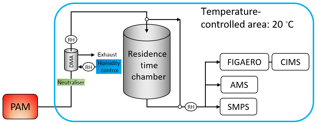
The acquisition of the data set investigated in this study was described in detail in Buchholz et al. (2019) and in the Supplement. The schematic overview of the set-up is shown in Fig. 1. Briefly, three types of SOA were formed via combined ozonolysis and photo-oxidation of α-pinene in an oxidative flow reactor (OFR). They are characterised as low, medium, and high O:C based on their elemental composition (oxygen-to-carbon (O:C) ratio of 0.53, 0.69, and 0.96, respectively, as derived from the aerosol mass spectrometer data). A nano differential mobility analyser (NanoDMA, TSI Inc.) was used to select a quasi-monodisperse particle distribution (with an electrical mobility diameter of 80 nm) and, at the same time, dilute the surrounding gas phase by orders of magnitude, which initiates isothermal evaporation at the NanoDMA outlet. The monodisperse particles were then filled into a stainless-steel residence time chamber (RTC) to study their isothermal evaporation behaviour by measuring the particle size in 1 h intervals for up to 10 h. Two sets of evaporation experiments were conducted for each SOA type, namely dry (RH < 2 %) and wet (RH 80 %). To achieve the different RH conditions and control the RH of the selected sample and in the RTC, only the RH of the sheath flow in the NanoDMA was adjusted. The conditions of α-pinene SOA formation in the OFR were not changed. The instruments, tubing, RTC, and OFR were flushed with particle-free purified air or nitrogen between experiments.

Figure 1 Schematic diagram of experimental set-up.

The chemical composition of the particles was investigated with a filter inlet for gases and aerosols (FIGAERO, Aerodyne Research Inc.; Lopez-Hilfiker et al., 2014) sampling unit in combination with a chemical ionisation mass spectrometer (CIMS, Aerodyne Research Inc.; Lee et al., 2014) using iodide as reagent ion. Samples were taken directly after the size selection (“fresh” particles: t_evap=0.25 h) and after 3–4 h of isothermal evaporation in the RTC (“RTC” particles: t_evap=4 h). Note that the evaporation time of 0.25 h for the “fresh” sample does not stem from residence in the RTC but rather from the collection time on the filter (see Sect. S1.1 in the Supplement for details). Due to this minimum evaporation time, the FIGAERO–CIMS measurements will underestimate the contribution of volatile compounds in the particles as they leave the OFR.

The combined analysis of the evaporation behaviour and FIGAERO–CIMS thermogram with the composition information in Buchholz et al. (2019) revealed increasing average desorption temperatures with increasing O:C ratio of the particles, while the overall particle volatility (measured by isothermal evaporation) decreased. The residual particles after isothermal evaporation in the RTC exhibited an increase in desorption temperature in all cases, which indicates that the more volatile species had left the particles. Under wet conditions, evaporation was enhanced due to the lowering of particle viscosity and, thus, kinetic transport limitations as described previously (D'Ambro et al., 2018; Wilson et al., 2015; Yli-Juuti et al., 2017). But in the high-O:C case, strong indications for aqueous-phase chemistry were found in the data, namely the shift of some ion thermograms to much higher desorption temperatures and a relative increase in low molecular weight (M_w) compounds. Thus, this data set is perfect for testing the performance of PMF with FIGAERO–CIMS data and determining whether PMF can capture the evaporation behaviour and separate it from aqueous-phase processes in the high-O:C case.

2.2 FIGAERO–CIMS measurements

It is necessary to understand the operation and data structure of FIGAERO–CIMS to comprehend the challenges of analysing this data with PMF. In the FIGAERO inlet, particles are collected on a polytetrafluoroethylene (PTFE) filter. A gradually heated nitrogen gas flow evaporates increasingly less-volatile compounds and transports them into the CIMS for detection. Hereafter, the resulting signal versus desorption temperature curves will be called ion thermogram for individual ions and total thermogram for the sum of all detected ions apart from the reagent ions. Each desorption cycle (“thermogram scan”) consists of the following three parts: the particle collection; the linear increase of the desorption temperature (here, ∼25 ^∘C $\to \sim \mathrm{190}$ ^∘C in 15 min); and a “soak” period at the highest temperature (here, > 190 ^∘C for 15 min). The soak period ensures that low-volatility compounds have been removed from the FIGAERO filter before the next sample is collected. Note that only the part of the thermogram with a near-linear increase in the desorption temperature can be used to derive volatility information. The relationship between a compound's desorption temperature, specifically T_max, and volatility (e.g. expressed as saturation vapour pressure) can be calibrated for a specific FIGAERO–CIMS set-up and temperature ramp by measuring, for example, polyethylene glycol aerosol with a range of molecular weights and volatilities (similar to the method described by Bannan et al., 2019).

The raw FIGAERO–CIMS data were processed by using tofTools, a MATLAB-based software package developed for analysing time-of-flight CIMS data (Junninen et al., 2010). The data were averaged to a 20 s time grid, and a baseline correction was applied before the high-resolution mass spectra data were fitted. The filter blank measurements were processed in the same fashion as the collected samples. For the PMF analysis, we did not subtract the filter blank measurements but instead added the corresponding filter blank thermograms to the data set to help with the identification of the background factors i.e. factors dominated by compounds from the instrument and/or filter background (more details on factor identification in Sect. 3.1).

Due to suboptimal settings in the instrument's ion guidance unit, an atypically high number of declustered ions (not containing the reagent ion iodide) were observed. This was discussed in detail in Buchholz et al. (2019). For this study, we will not make any assumptions about the declustering process and treat the iodide clusters and declustered ions as separate variables. However, this impacts neither the application of PMF to the data set nor the validity of this method for other data sets as the variables (ions) are all treated independently in the model, and the variables with the same behaviour will be grouped into the same factor.

2.3 Positive matrix factorisation (PMF)

2.3.1 Working principles of PMF

Since its introduction by Paatero and Tapper (1994), PMF has been established as a useful tool for analysing long time series of mass spectra data mostly from ambient observations.

In the PMF model, it is assumed that the measured data can be expressed by the combination of an (unknown) number p of constant source profiles with varying concentrations over time (Ulbrich et al., 2009). This can be mathematically expressed as follows:

$$\begin{array}{}\text{(1)}& \mathbf{X}=\mathbf{GF}+\mathbf{E},\end{array}$$

where X is a m×n matrix containing the measured mass spectra with m rows of mass spectra (“observations”), which are each averaged over 20 s of measurement time in the CIMS, and n columns representing the time series of one specific ion. G is a m×p matrix containing the factor time series as columns. The rows of the p×n matrix F contain the factor mass spectra, and then the m×n matrix E contains the residuals between the measured data and the fitted values. No a priori information about the values of G and F or the number of factors (p) is required, but the user has to decide which solution (i.e. how many factors) characterises the data best. To account for uncertainties in the measurement data, the PMF model weights the data points with their measurement error (S_ij). Values for G and F are constrained to be positive and are iteratively found by minimising the quantity, Q, with a least square algorithm (Paatero and Tapper, 1994) as follows:

$$\begin{array}{}\text{(2)}& Q=\sum _{j=\mathrm{1}}^m\sum _{i=\mathrm{1}}^n{\left({\displaystyle \frac{{\mathbf{E}}_{ij}}{{\mathbf{S}}_{ij}}}\right)}^{\mathrm{2}},\end{array}$$

where S_ij is the error (uncertainty) of each measurement data point. In an ideal case, the Q value of the model should approach the expected Q value (Q_exp) that is equal to the degree of freedom of the model solution. For mass spectra data, this is approximately equal to the size of the original data matrix, X, as follows:

$$\begin{array}{}\text{(3)}& Q_{\exp }\approx n\cdot m.\end{array}$$

Different algorithms have been developed to solve the PMF model (e.g. Hoyer, 2004; Lu and Wu, 2004; Paatero, 1999). In this study, we used the PMF2 algorithm with robust least square optimisation, which is included in the PMF Evaluation Tool (PET, Ulbrich et al., 2009) for Igor Pro 7 (WaveMetrics, Inc., Portland, Oregon). We calculated solutions with 1 to 12 factors. For each solution, 5 rotations (f_peak−1.0 to +1.0) were calculated, and 6 different seed values were tested for each original solution (f_peak=0).

As an additional measure for the goodness of fit, we calculated the fraction of explained absolute variance (Ratio_exp) as follows:

$$\begin{array}{}\text{(4)}& {\displaystyle }{\mathrm{absVar}}_{\mathrm{total}}=\sum _{ij}\left|{\mathbf{X}}_{ij}-\stackrel{\mathrm{‾}}{X_i}\right|\text{(5)}& {\displaystyle }{\mathrm{absVar}}_{\mathrm{explained}}=\sum _{ij}\left|{\mathbf{R}}_{ij}-\stackrel{\mathrm{‾}}{X_i}\right|\text{(6)}& {\displaystyle }{\mathrm{Ratio}}_{\exp }={\displaystyle \frac{{\mathrm{absVar}}_{\mathrm{explained}}}{{\mathrm{absVar}}_{\mathrm{total}}}},\end{array}$$

where R_ij is the value in the reconstructed data matrix (R=GF) for each ion i and observation j, $\stackrel{\mathrm{‾}}{X_i}$ is the average measured value of the ion i, and absVar_total and absVar_explained are the total and explained absolute variance. Note that we use the absolute distance between the average values and the measured or reconstructed data instead of the square of this distance.

PMF has been widely used for analysing the time series of mass spectra data in the atmospheric science community. However, the model does not utilise the information of the time axis in the optimisation process. Rather, it is a method that can be used to analyse a set of mass spectra, which were obtained at different time points during the desorption cycle of FIGAERO, and for different particle sampling conditions. This means that PMF will create the same model output if the x values in the data set are a real time series (Fig. 2b), a temperature ramp (Fig. 2c), or simply an index with numbers (Fig. 2a). Thus, data from separate thermogram scans with FIGAERO–CIMS can be combined to larger data sets and analysed together with PMF. Analysing multiple thermogram scans together has the advantage that more data points are utilised to identify the factors (90 mass spectra for each thermogram in this case) and that factors can be directly compared between scans. The real time series/temperature ramp is only of interest when evaluating the model output for the interpretation of the identified factors and comparing their desorption temperature profiles between thermogram scans. In the graphic presentation of these combined “time series” (e.g. Fig. 4), a data index was used as the x values, which is the desorption temperature of each thermogram plus an offset (200 per thermogram). This choice of x values preserves the shape of the thermogram in the desorption temperature space. The individual thermograms are marked with roman numerals and the sampling conditions are given in the figure captions. For an easier comparison of the shape of the desorption behaviour of the factors, they are plotted individually for each SOA type (e.g. Fig. 5).

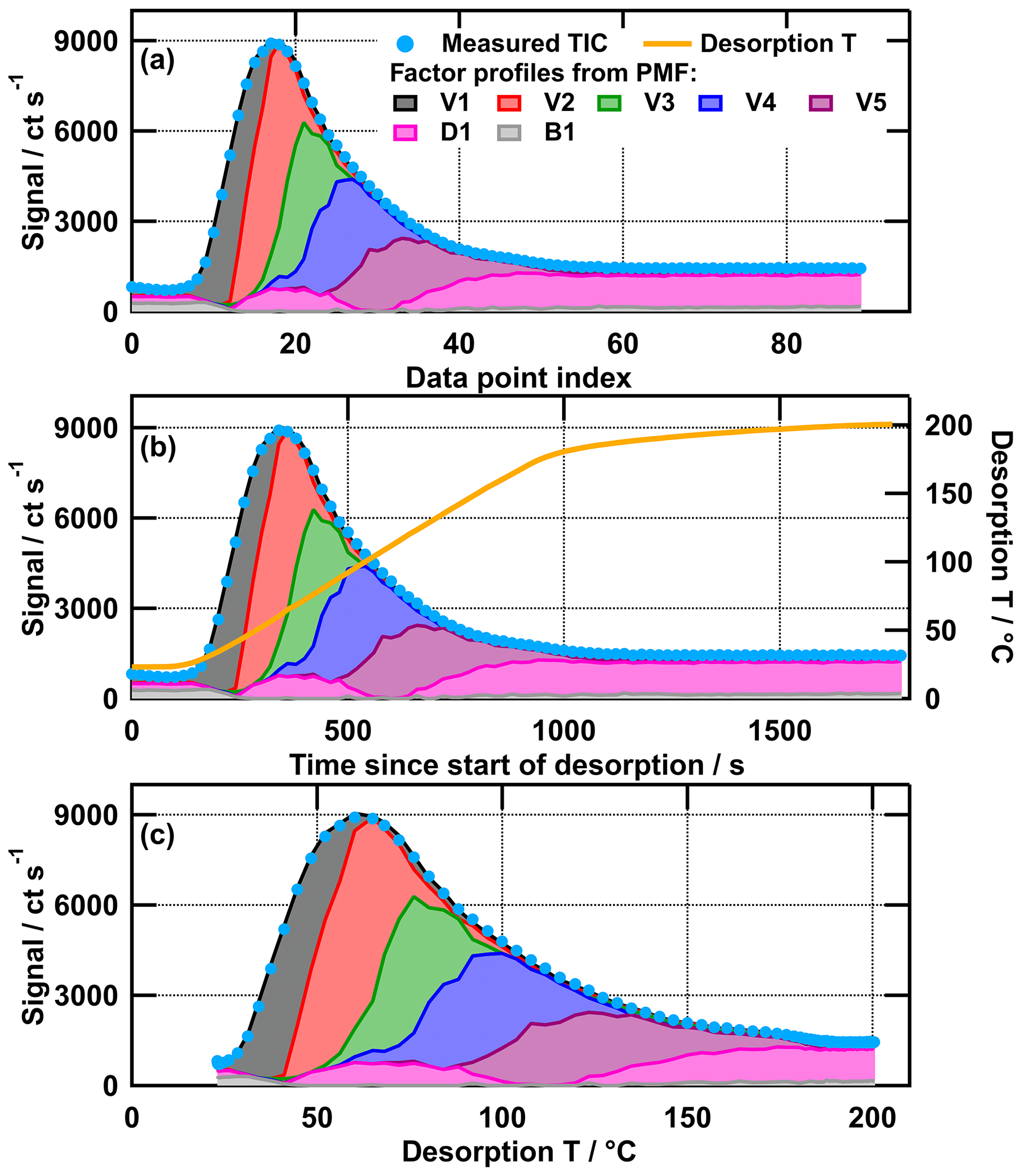
Figure 2 Measured total ion thermogram with the colour-coded contributions of PMF model output factors for the medium-O:C wet (t_evap=4 h) case plotted against data point index (a); time since start of desorption (b); and desorption temperature (c). Note that the desorption temperature ramp (b) is not increasing linearly after ∼1000 s. This “soak” period ensures that all organic material is removed from the filter before the next collection.

When performing PMF with the combined data set with all available thermogram scans, the large number of factors (13 or more) necessary to explain the observed variability complicates the analysis and interpretation (see the case study in Sect. S1.4). Thus, the thermogram scans were grouped by SOA type (i.e. t_evap=0.25 h and 4 h particles, dry and wet conditions of one SOA type: four thermogram scans per group). This pre-grouping reduced the number of factors in each group enhancing their interpretability while still enabling a direct investigation of the changes due to the evaporation and/or humidification for one SOA type. But, generally, splitting the data by SOA type or even knowing about different SOA types and/or sources in the data is not a requirement for analysing a thermogram data set with PMF.

2.3.2 Error schemes for PMF

To perform the PMF analysis, a data error S_ij must be defined. As seen in Eq. (2), the S_ij values have a strong influence on the outcome of the PMF model. The measurement error can be understood as a weighting mechanism that gives more weight to data points with less uncertainty (Paatero and Hopke, 2003). Ideally, S_ij is the true measurement error of the data set. For gas-phase CIMS data, Yan et al. (2016) suggested calculating the measurement error by assuming a Poisson-type distribution of the counting error as follows:

$$\begin{array}{}\text{(7)}& {\mathbf{S}}_{ij}=a\cdot \sqrt{{\displaystyle \frac{{\mathbf{X}}_{ij}}{t_{\mathrm{s}}}}}+{\mathit{\sigma }}_{\mathrm{noise},i},\end{array}$$

where X_ij is the signal intensity of the ion i, t_s is the sampling (averaging) interval in s, and σ_noise,i is the electronic noise for ion i. We applied a procedure equivalent to the one introduced by Yan et al. (2016) to derive the parameter a from analysing the distribution of signal noise. The detailed calculation for this type of error is given in the Supplement. The resulting error values (Poisson-like – “PLerror”) will trace the shape of the thermogram signal with higher absolute values for those parts of the thermogram that have higher intensity (i.e. the “peak”) and give less weight to this region (Fig. S1 in the Supplement). This is the correct approach for the analysis of long time series data in which rapid changes are most likely caused by instrument noise or data outliers.

For FIGAERO–CIMS thermograms, the main information lies in the rapidly increasing and decreasing part of the data (i.e. the “peak”; data points 10–50 in Fig. 2a) when the compounds are desorbing from the FIGAERO filter and not in the slowly changing (or constant) part at high desorption temperatures (i.e. the “tail”; data points 50–90 in Fig. 2a). During this analysis it was found that the thermal desorption peaks could not be modelled well with error values calculated using Eq. (7) (see Sect. 2.3.3 and Appendix A). Thus, a new error scheme that allowed for an increased weighting of the thermal desorption peaks was also tested. In this scheme, a constant error value corresponding to the noise in the data at the end of the thermogram scan is used for each thermogram scan (constant noise – “CNerror”) as follows:

$$\begin{array}{}\text{(8)}& {\mathbf{S}}_{ij}={\mathit{\sigma }}_{\mathrm{noise},i},\end{array}$$

where σ_noise,i of each ion i is calculated in the same way as for the PLerror (see the Supplement for details). Note that by omitting the first term in Eq. (7), Eq. (8) does not correspond to the true measurement error of the FIGAERO–CIMS data. Rather, it is the simplest way of weighting the PMF runs to put more emphasis on each thermogram peak and less on the fronts and tails (Fig. S1 shows an example of the values for the two error schemes for one exemplary ion). The signal-to-noise values are up to 3 orders of magnitude higher in the peak region for the CNerror case, which clearly gives them a stronger weight in the optimisation. As a direct consequence of the modified error value, the value for Q∕Q_exp is not expected to approach 1 but will instead reach a larger (used error values smaller than real measurement error) or smaller (used error values larger than real measurement error) value. Thus, most solutions from PMF with PLerror will have (much) lower Q and Q∕Q_exp values than any solution from PMF with CNerror. This also means that comparing the absolute Q or Q∕Q_exp values between results from the different error schemes is not meaningful as a higher absolute error value will result in a lower Q value.

2.3.3 Selection of error scheme and number of factors (“best” solution)

Before the “best” solution from PMF can be identified by investigating the factor profiles and spectra, the impact of the two different error schemes on the PMF output needs to be determined by running PMF for all combined data sets with both error schemes and comparing the output. Since the comparison of the Q∕Q_exp values between the error schemes is not meaningful, as pointed out previously, the fraction of explained variance (Ratio_exp) and the reconstruction of the characteristic shape of the thermograms (i.e. time series of residuals) were the decisive criteria. In addition to the single Q∕Q_exp value summed over all ions and observations (i.e. mass spectra) in each data set, we calculated the time series of the Q contributions (Q_j) summed over all ions for each observation (mass spectrum), j, to identify which periods in the data set were not captured well by the investigated PMF solution. The calculation is as follows:

$$\begin{array}{}\text{(9)}& Q_j=\sum _{i=\mathrm{1}}^n{\left({\displaystyle \frac{{\mathbf{E}}_{ij}}{{\mathbf{S}}_{ij}}}\right)}^{\mathrm{2}}.\end{array}$$

Similarly, we calculated Q_i as the value sum over all observations (mass spectra), j, as follows, to investigate which ion has the strongest contribution to the overall Q value:

$$\begin{array}{}\text{(10)}& Q_i=\sum _{j=\mathrm{1}}^m{\left({\displaystyle \frac{{\mathbf{E}}_{ij}}{{\mathbf{S}}_{ij}}}\right)}^{\mathrm{2}}.\end{array}$$

For a given number of factors, the CNerror scheme results in higher Ratio_exp values than the PLerror (Fig. 3), i.e. a larger fraction of the observed variance is captured by the model. With the PLerror the maximum Ratio_exp is 0.9 – even with up to 12 factors – while the values for Ratio_exp with the CNerror are already > 0.95 with 7 factors.

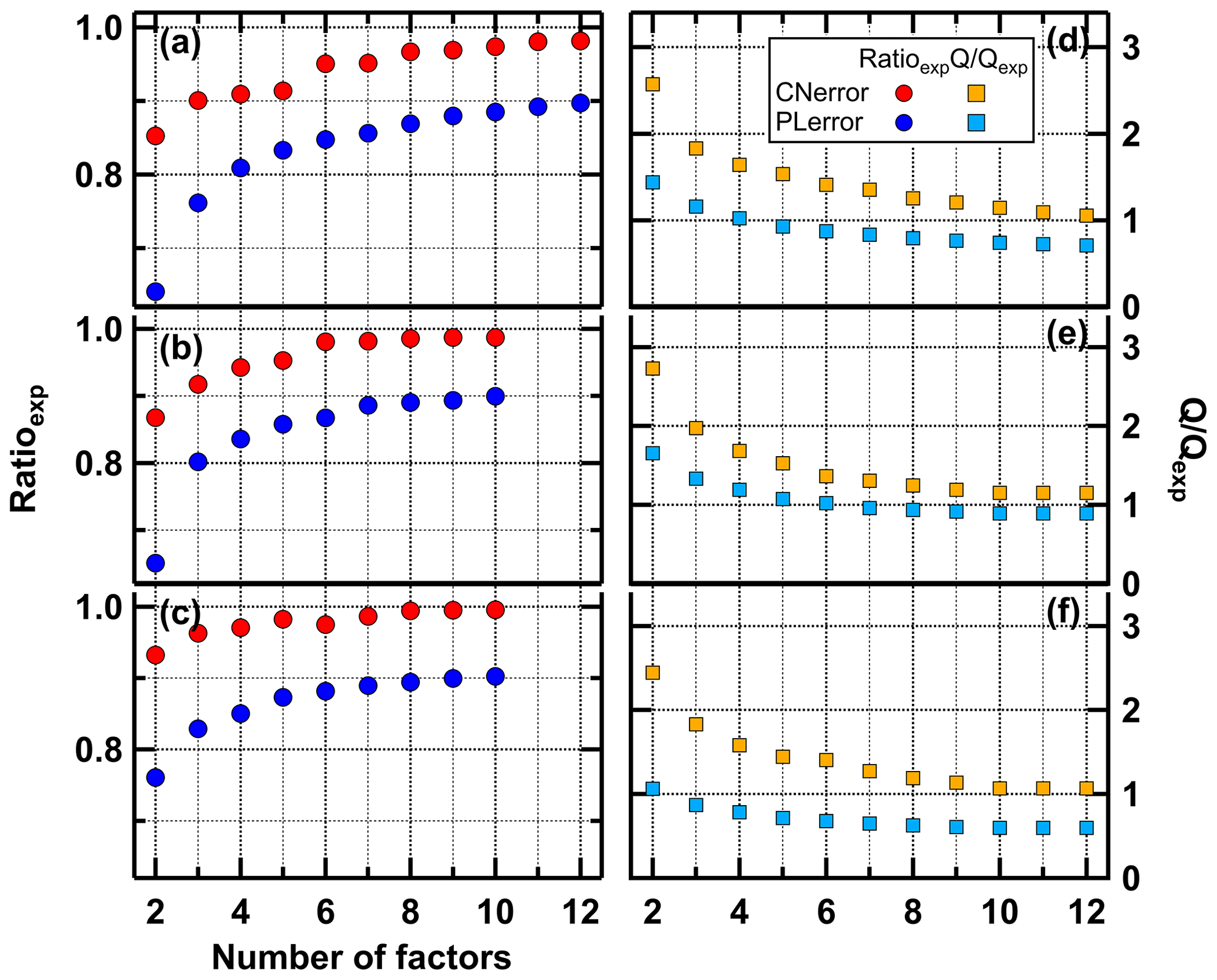
Figure 3 Fraction of explained variance (Ratio_exp, a–c) and Q∕Q_exp values (d–f) for the low- (a), medium- (b), and high-O:C (c) data set for PLerror (blue) and CNerror (red).

Figure 4 Total ion thermogram (a), residuals (b, d), and Q_j∕Q_exp values (c, e) as time series for solutions with 6, 7, or 10 factors for PMF run with CNerror (b, c – yellow background) and PLerror (d, e – blue background). The data set contains thermogram scans for the high-O:C SOA particles from the following sampling conditions: dry – t_evap=0.25 h (I); dry – t_evap=4 h(II); wet – t_evap=0.25 h (III); and wet – t_evap=4 h (IV). Note that the y-axis scaling is the same in panels (b) and (d), but it is 10 times smaller in (e) than in (c).

To highlight the differences in the behaviour of the two error schemes, we display the time series of the residual and Q_j values in Fig. 4 for the high-O:C case for three solutions (6, 7, and 10 factors). With the PLerror, the residuals are much larger than in the CNerror case (panels b and d). But, due to the larger values of S_ij in the PLerror case, the Q∕Q_exp values (panels c and e) are much smaller. Thus, the optimisation algorithm sees no need to further improve the model in the PLerror case. In contrast, the smaller unscaled residual in the 6-factor solution with the CNerror leads to much higher Q∕Q_exp values, especially in the peaks of thermograms III and IV. Here, the addition of 1 factor (from 6 to 7) improves both the residual and the Q_j∕Q_exp values, and the new factor captures a characteristic behaviour that we discuss in Sect. 3.3.

This analysis, together with the more detailed case study in Appendix A, leads us to the conclusion that, for this study and data set, the CNerror reconstructed the measured data best and yielded the most interpretable results. Thus, hereafter we only present the results from PMF runs with the CNerror scheme.

The advantage of PMF, that no a priori information about F, G, and p is needed for the analysis, is also a disadvantage. There is no absolute criterion for which number of factors (p) is correct or “best”, but the chosen value strongly impacts the interpretation of the factors and their profiles. In the ideal case, when the true measurement errors are used, Q∕Q_exp approaches 1, and a solution with Q∕Q_exp close enough to 1 may be considered as the “best” or most correct. But, as we explained previously, PMF performed much better for FIGAERO–CIMS data when the “unrealistic” CNerror scheme was used; thus Q∕Q_exp are not necessarily meaningful. However, the shape of the Q∕Q_exp versus the number of factors curve can be used to judge the impact of introducing another factor; i.e. a large change in Q∕Q_exp values suggest that the new factor explains a large fraction of the variability in the data (Ulbrich et al., 2009). We investigated this for the PMF runs for each SOA type (Figs. 3 and S2). The largest changes in Q∕Q_exp are already achieved by increasing the factors from 2 to 3. Further factor addition leads to a steady decrease of Q∕Q_exp. In this case, the Ratio_exp values are more helpful. Strong increases of Ratio_exp are observed when increasing the number of factors to 6 (medium- and high-O:C cases) or 8 (low-O:C case).

As shown by Yan et al. (2016) for gas-phase CIMS data, a solution with a low overall Q∕Q_exp value may still have large variations in the scaled residual with time or with different ions. We carefully investigated the time series (Q_j∕Q_exp) of individual ions (e.g. ${\mathrm{C}}_{\mathrm{5}}{\mathrm{H}}_{\mathrm{5}}{\mathrm{O}}_{\mathrm{6}}^{-}$ in Fig. A1b and c) in particular and present the details of this case study in Appendix A. There were a few specific ions for each SOA type that were not captured well in the data set until a certain number of factors was chosen (e.g. 7 in the high-O:C case) – even if the overall fraction of explained variance for the solutions was already larger than 95 % and changed very little with further factor additions. We decided to choose the PMF solution with the smallest number of factors that still described the characteristic behaviour of most ion thermograms. These were the solutions with 9, 7, and 7 factors for the low-, medium-, and high-O:C cases, respectively.

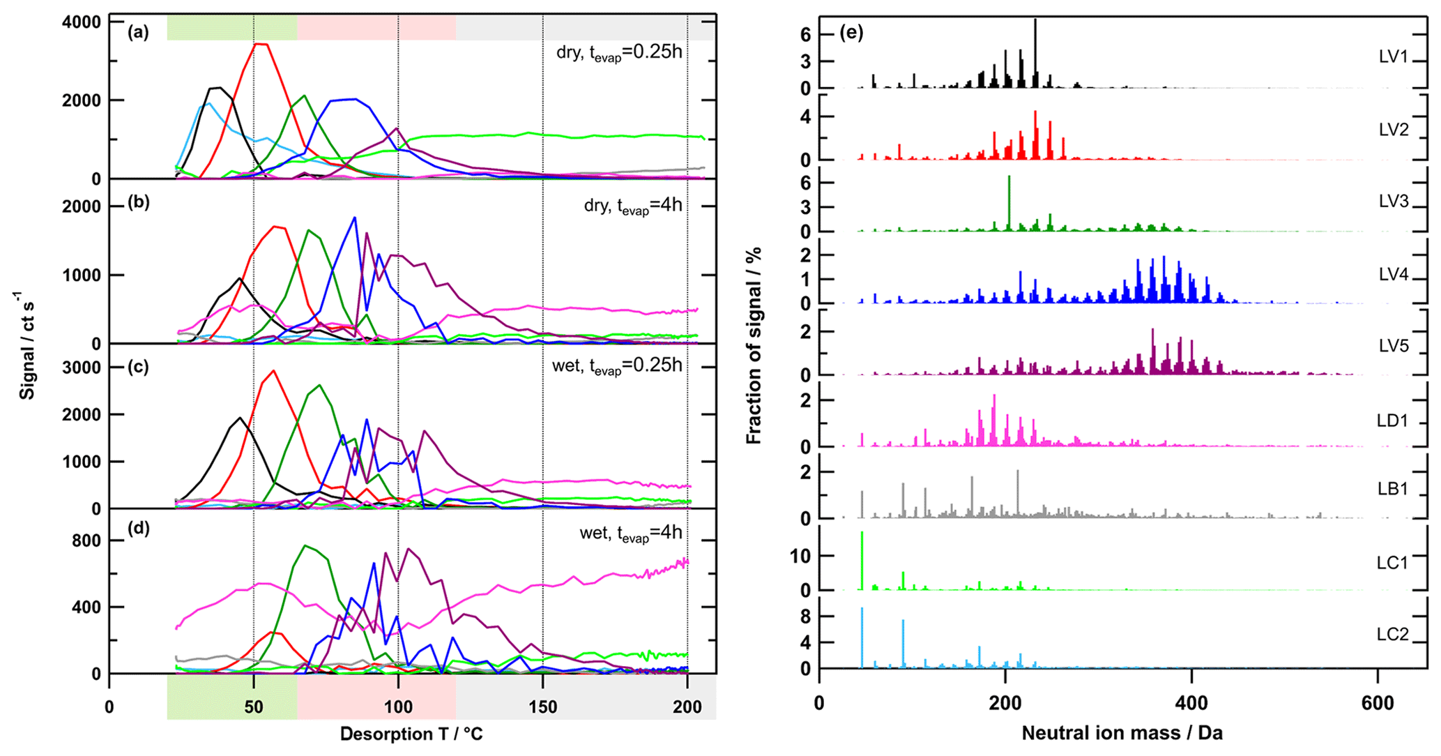
Figure 5 Factor thermograms (a–d) and factor mass spectra (e) for the 9-factor solution for the low-O:C case. Each factor mass spectrum is normalised. The colour code is the same for both panels. Background colours in the panel on the left indicate volatility classifications according to Donahue et al. (2006) and are derived from T_max–$C_{\mathrm{sat}}^{\ast }$ calibrations (green: semi-volatile organic compounds (SVOCs), red: low-volatility organic compounds (LVOCs), and grey: extremely low volatility organic compounds (ELVOCs)). Note the different scaling for the y axes in (a)–(d).

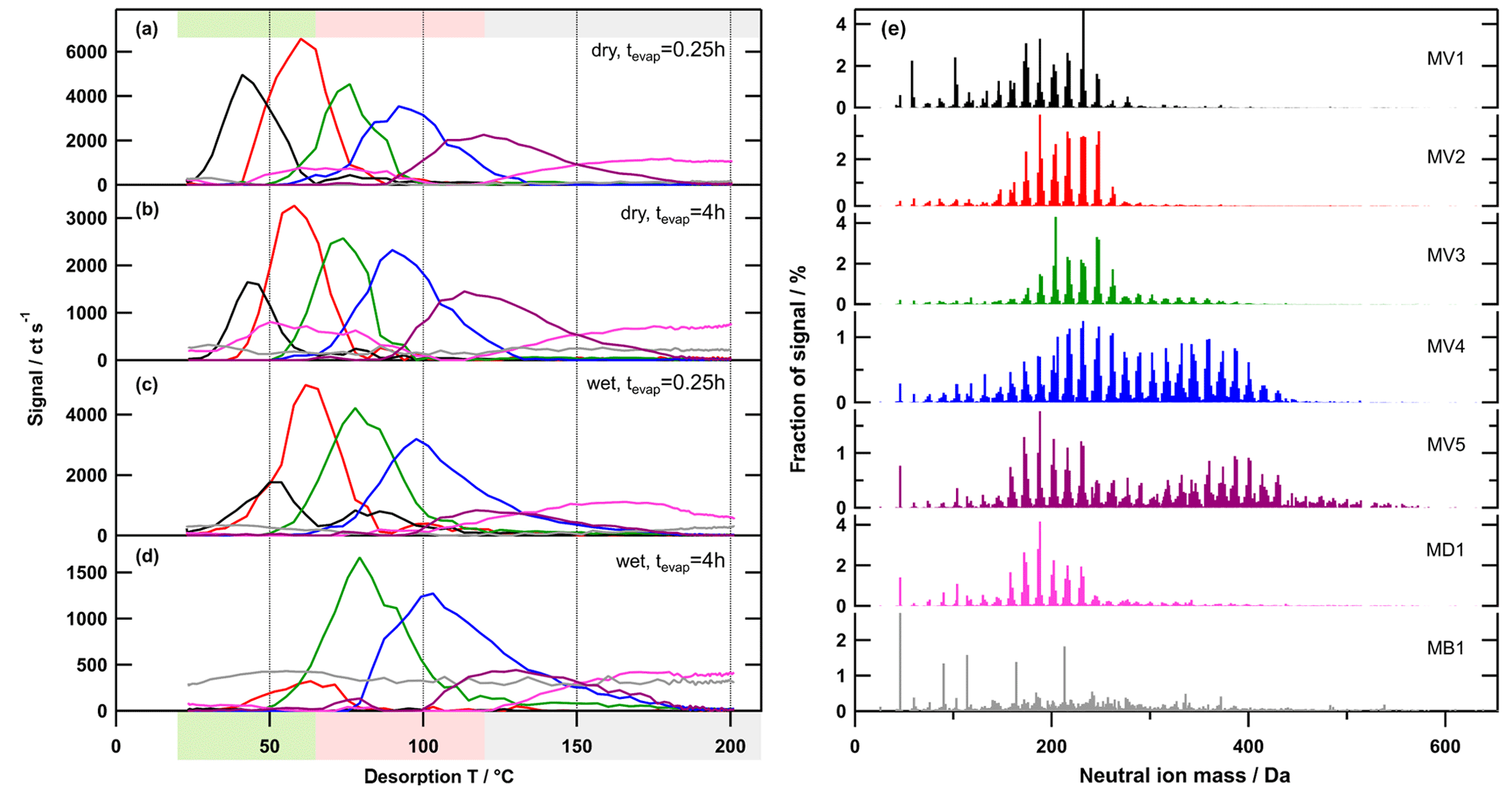
Figure 6 Factor thermograms (a–d) and factor mass spectra (e) for the 7-factor solution for the medium-O:C case. Each factor mass spectrum is normalised. The colour code is the same for both panels. Background colours in the panel on the left indicate the volatility classification derived from T_max–$C_{\mathrm{sat}}^{\ast }$ calibrations (green – SVOC; red – LVOC; and grey – ELVOC). Note the different scaling for the y axes in (a)–(d).

3 Results and discussion

3.1 PMF-factor interpretation

The three evaporation data sets (one for each SOA type) were analysed with PMF by using the CNerror scheme and the results for the “best” solutions chosen are shown in Figs. 5, 6, and 7 (and with “stacked” factor contribution in Figs. S4, S5, and S6). In the following paragraphs, the first letter in the labels of factors indicates whether they are from the low- (L), medium- (M), or high (H)-O:C case, and the second letter identifies the factor type (V, B, D, and C; see below).

Generally, there were the following three main types of thermogram profiles for all factors: volatility class (type V) with a single, distinct peak (LV1 – 5, MV1 – 5, and HV1 – 5); background (type B) with mostly constant contribution over the full T_desorp range (LB1, MB1, and HB1); and decomposition (type D) with mostly very broad peaks at T_desorp < 65 ^∘C and an increase at T_desorp > 110 ^∘C (LD1, MD1, and HD1).

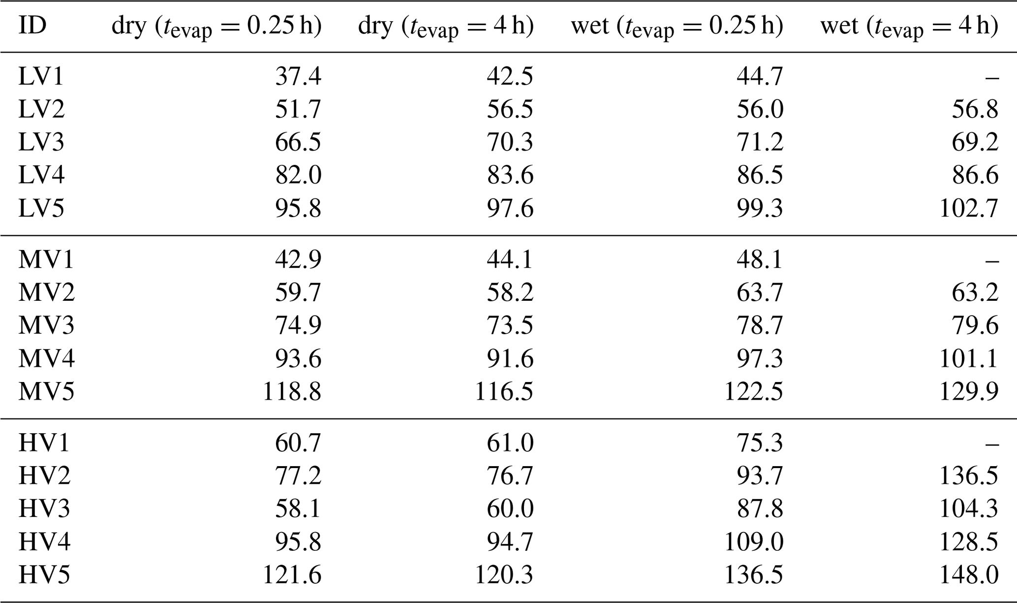
Factors of type V do not contribute to the filter blank thermograms (Fig. S3), which indicates that these factors are linked to compounds only present in the sampled aerosol particles. With the exception of the high-O:C wet case (which we discuss in detail in Sect. 3.3), the peak position (T_max) of type-V factors changes very little with aerosol age or water content (Table 2). Only the contribution of these factors to the total signal changes with isothermal evaporation or humidification. For each type-V factor, we could identify ions with thermogram shapes similar to the thermogram profile of the individual factors. This means that especially the type-V factors at high desorption temperature are not merely a better mathematical description of the tails of some ion thermograms, but they represent real compounds desorbing from the FIGAERO filter at high desorption temperatures. Thus, we interpret the type-V factors as volatility classes. Compounds with the same thermal desorption behaviour (i.e. volatility) are grouped into one type-V factor that is characterised by its T_max value. Note that for the three different SOA types the starting particle composition was significantly different. So, even if the T_max values for 2 factors of different SOA types, e.g. LV2, MV2, and HV1 (dry cases), only differ by ∼5 ^∘C, the compounds contributing to them are not the same; i.e. the factor mass spectra for LV2, MV2, and HV1 are significantly different. We elaborate on the reasons for these differences in Sect. S1.3 and S1.4.

Type-B factors show contributions to the signal of sample thermograms and filter blanks (Fig. S3). For LB1, MB1, and HB1, the very shallow thermogram profile and the similar absolute signal strength despite different mass loadings on the FIGAERO filter indicate that these are instrument background factors. For some samples, especially those with high overall filter loading, the factor thermograms of the type-B factors show a decrease to almost 0 for T_desorp ∼60–∼120 ^∘C. This may indicate that part of the background signal in this temperature range is assigned to other factors (“factor blending/mixing”). Since the overall background in these few cases is 200–400 ct s⁻¹ while the signals of the type-V factors are more than 10 times higher, this factor blending will have a minor effect on the shape and T_max values of the type-V factors and thus the interpretation of the PMF solution. For the parts of the thermograms with lower signal strength and samples with low overall mass loading on the filter, the signal of the type-B factors stays constant at a value that is comparable to values observed for the filter blank samples. For all SOA types, the mass spectra of these factors are dominated by single ions typically associated with the FIGAERO–CIMS background (e.g. fluorine-containing compounds, formic acid, and lactic acid). According to the uncentred correlation method (contrast angle or dot product) MB1 and HB1 are reasonably similar. For the low-O:C case, some of the instrument background is apparently assigned to the contamination factors (LC1 and 2; see below), which decreases the degree of similarity between LB1 and the other type-B factors.

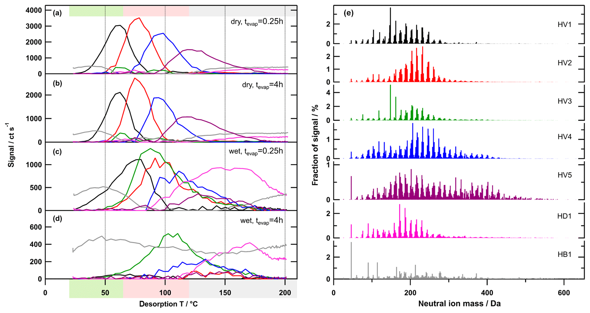
Figure 7 Factor thermograms (a–d) and factor mass spectra (e) for the 7-factor solution of the high-O:C case. Each factor mass spectrum is normalised. The colour code is the same for both panels. Background colours in the panel on the left indicate the volatility classification derived from T_max–$C_{\mathrm{sat}}^{\ast }$ calibrations (green – SVOC; red – LVOC; and grey – ELVOC). Note the different scaling for the y axes in (a)–(d).

Type-D factors are the most difficult to interpret as they contribute to the signal for both the filter blank and sample thermograms, but the contribution can vary with the collected mass loading on the filter for sample thermograms. The factor mass spectra (LD1, MD1, and HD1) mostly show contributions from ions with M_w < 200 Da, but the thermogram profiles exhibit a strong increase at T_desorp > 110 ^∘C, especially in filter blank thermograms. This suggests that the detected low M_w compounds in these factors are thermal decomposition products of larger, low-volatility compounds that are thermally unstable. But in some cases (e.g. medium-O:C dry – t_evap=0.25 h and 4 h; Fig. 6a and b) a second peak occurs at much lower T_desorp (< 65 ^∘C), which is in the range where compounds of the detected composition are expected to desorb. This suggests that the ions grouped into the type-D factors can stem from two “sources”, namely direct desorption (T_desorp < ∼100 ^∘C) and thermal decomposition (T_desorp > ∼100 ^∘C), and PMF is not able to separate them because either their composition or their desorption behaviour is too similar. Consequently, type-D factors have to be carefully analysed and interpreted as desorption at low T_desorp and decomposition at high T_desorp. Also, the instrument background contribution needs to be estimated from the filter blank thermograms. For the low-O:C case, LD1 is dominated by compounds coming from the filter/instrument background as the factor thermogram does not change with the collected sample mass, and there is still a contribution from the factor below T_desorp < 100 ^∘C after 4 h of isothermal evaporation (Fig. S3a). In the medium-O:C case, the direct desorption part (T_desorp < 100 ^∘C) of MD1 is removed with isothermal evaporation, which suggests that at least this part of the factor stems from the collected sample and not just the instrument/filter background. The high-O:C case is discussed in Sect. 3.3 below.

For the low-O:C dry (t_evap=0.25 h) sample, 2 additional factors (type C) were found. The factor mass spectra of LC1 and 2 are dominated by extremely high signals for formic and lactic acid, which are typically strong indications of a contamination on the FIGAERO filter due to handling. Retrospectively, we could not determine what happened to this specific sample collection to cause this obvious contamination, but the FIGAERO filter was replaced between this and the next sample collection, and several heating cycles were performed to ensure that no other sample was affected. However, since PMF has identified the ions affected by this contamination and grouped them into LC1 and 2, these 2 factors can be omitted from further analysis and remove the bias caused by the contamination.

Note that almost the same factors are produced by PMF regardless of whether the filter blank measurements are added to the data sets or not. This shows that PMF can be a very helpful tool for data interpretation when no reliable instrument background measurements are available or if the background varies strongly between samples. Then the identification of the type-B, type-D, and type-C factors has to rely on the factor thermograms and factor mass spectra.

Figure 8 Contribution of type-V factors to total signal for low- (a), medium- (b), and high-O:C cases (c). The x axis is the average volume fraction remaining (VFR) after comparable time intervals of isothermal evaporation observed in separate RTC experiments. Orange and blue arrows indicate the change from t_evap=0.25 h to t_evap=4 h particles for dry and wet conditions, respectively. Note that the colour code is the same in all panels, but LV1 is not equal to MV1, etc. VFR values are from isothermal evaporation measurements described in Buchholz et al. (2019). Average T_max values are for the comparison of the volatility of the factors. Detailed values are given in Table 2.

3.2 Composition changes due to evaporation

One set of type-V factors (i.e. volatility classes) was identified and separated from the instrument background contributions for each data set consisting of one SOA type sampled after different time intervals of isothermal evaporation under dry and wet conditions. The contribution of a single factor to the total signal is calculated as the ratio of the integral of the thermogram of this factor to the total signal. The relative contribution of factors V1–V5 for each sampling condition is shown in Fig. 8 and is plotted against the volume fraction remaining (VFR) that was measured in separate isothermal evaporation measurements (VFR values from Buchholz et al., 2019). The corresponding figure with absolute signal contributions is shown in the Supplement (Fig. S7). Note that the residual particles after isothermal evaporation or humidification were collected on the FIGAERO filter. This means that, with decreasing VFR, a larger fraction of the particle mass evaporated prior to the FIGAERO–CIMS measurements. In the low- and medium-O:C cases (Fig. 8a and b), the relative contributions of MV1 and 2, and LV1 and 2 (T_max in the range of semi-volatile organic compounds, SVOCs), decreased with decreasing VFR while those of LV3–5 and MV3–5 (T_max in the range of low- and extremely low volatility organic compounds, LVOCs and ELVOCs) increased. During 4 h of dry isothermal evaporation, a similar volume fraction was removed as in 0.25 h of isothermal evaporation under wet conditions. The very similar relative contribution of the type-V factors in these two samples suggests that the observed changes in chemical composition in the particles are indeed connected to the change in VFR (i.e. how much of the volatile material was removed before sampling) and are not directly driven by other water-induced processes. For these SOA types, the main process during physical ageing in the RTC (i.e. long residence time in clean air) under dry and wet conditions was isothermal particle evaporation. In this case, the particulate water mostly decreased the viscosity in the particles, thus decreasing the kinetic transport limitations in the particle phase and increasing evaporation. This observation is in agreement with previous interpretations of this and other comparable data sets (Buchholz et al., 2019; Yli-Juuti et al., 2017). The high-O:C case (Fig. 8c) will be discussed in Sect. 3.3.

Table 1 Signal-weighted average values of elemental composition, O:C, OSc, and the contribution of C > 10 compounds for all factors.

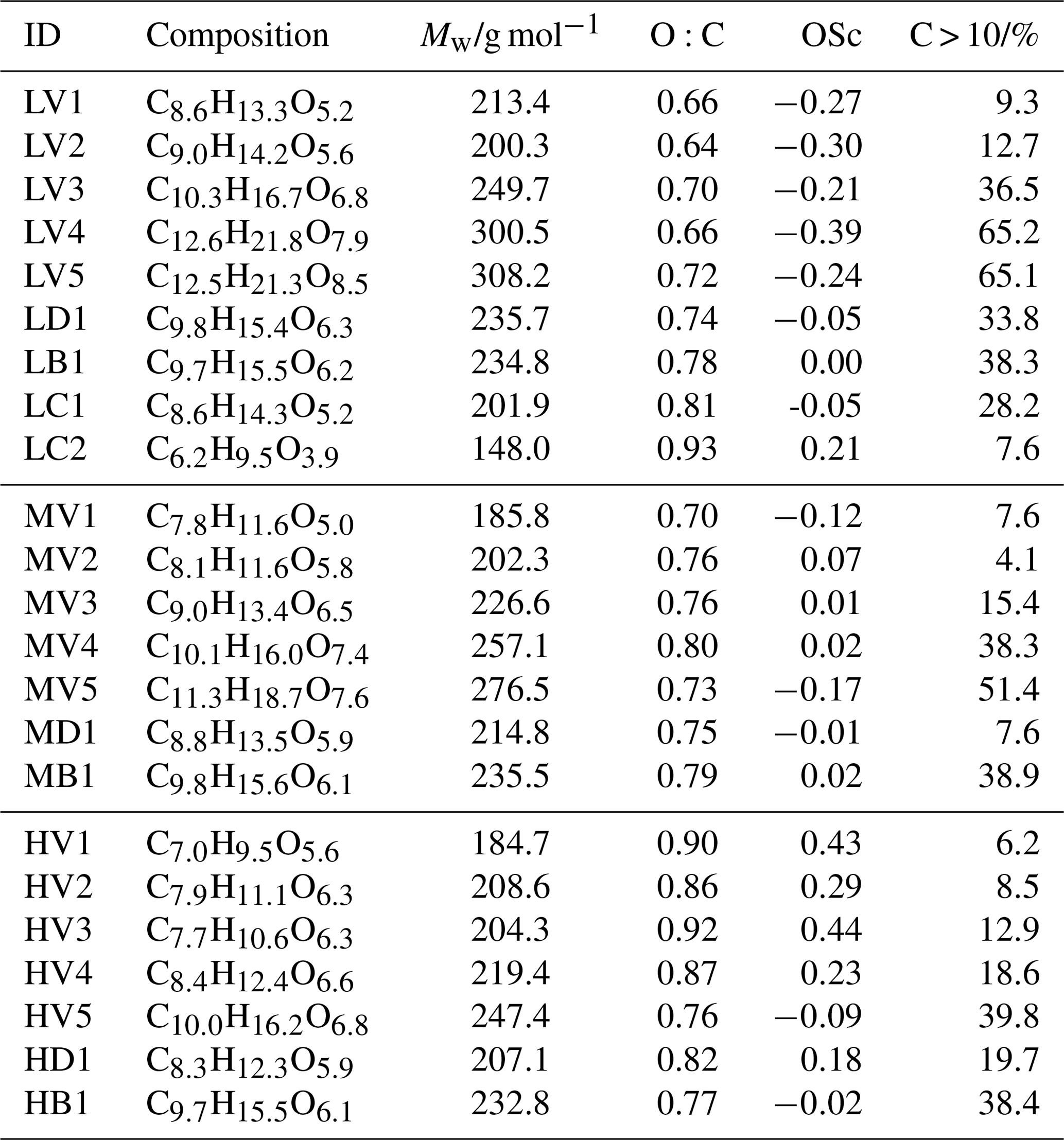
Table 2 T_max values for all type-V factors. The “–” symbol indicates that there was not enough signal to determine the T_max value.

The detailed changes in particle composition, due to isothermal evaporation, can be derived from the factor contribution by analysing the trends in the factor mass spectra. With increasing T_max of the factors (i.e. decreasing volatility), the average M_w as well as the carbon-chain length and the number of oxygen increased continuously from V1 to V5 (Table 1). The contribution of compounds with more than 10 carbon atoms (C > 10) also increased, which suggests an increasing contribution of dimers/oligomers. This may explain why no clear trend could be observed for the type-V factors in the O:C (or OS_c) values. While the lower volatility compounds did indeed contain more oxygen, the simultaneous increase of the carbon-chain length seems to compensate for this, which results in no obvious systematic increase in the O:C ratios. Thus, we observe a correlation of the volatility with average M_w but not with the average O:C ratio of the factors.

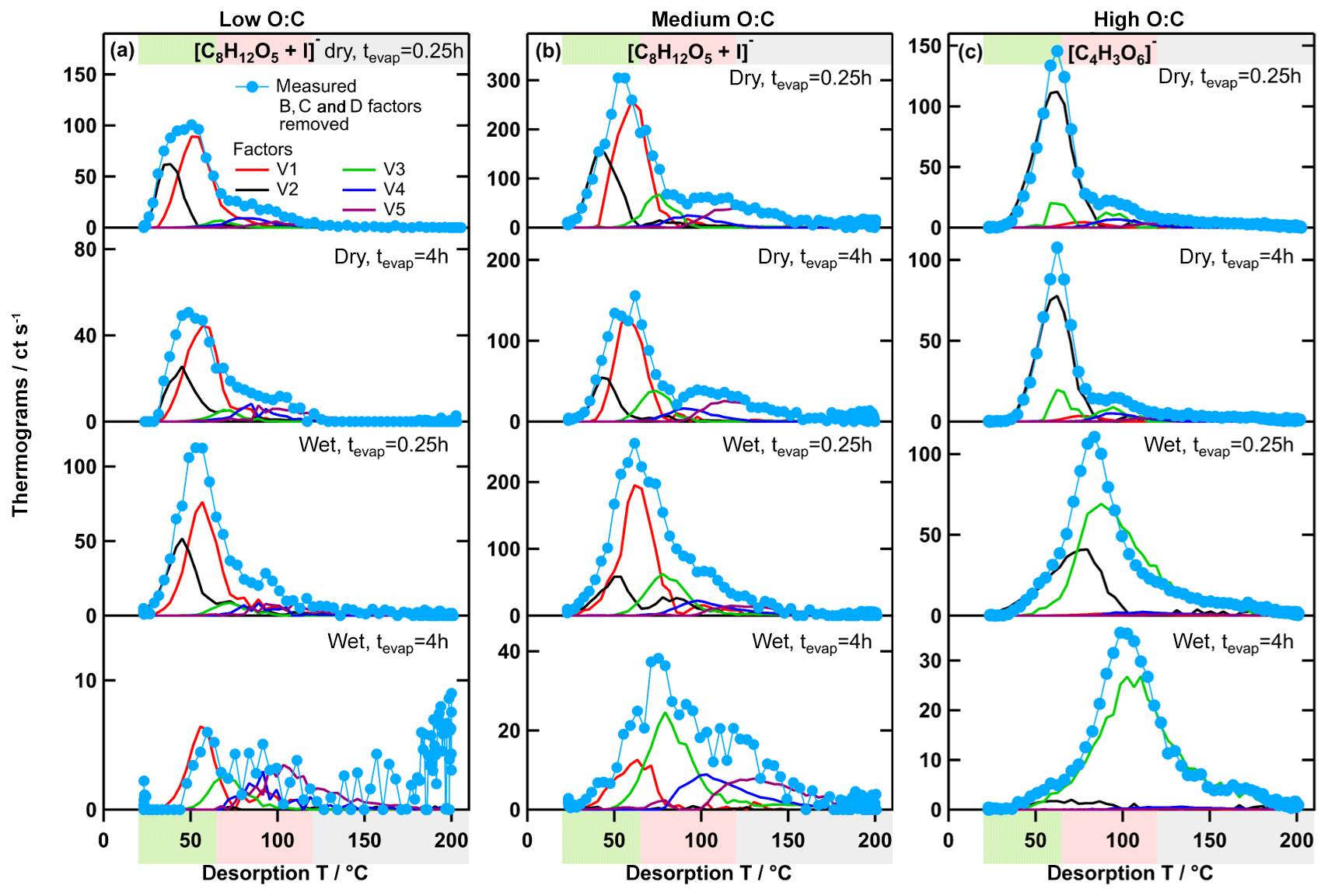
Figure 9 Measured ion thermograms and factor thermograms for ion [C₈H₁₂O₅+I]⁻ in the low- (a) and medium-O:C cases (b) and ${\mathrm{C}}_{\mathrm{4}}{\mathrm{H}}_{\mathrm{3}}{\mathrm{O}}_{\mathrm{6}}^{-}$ in the high-O:C case (c). Note that the contributions of the type-B, type-C, and type-D factors were subtracted from the measured ion thermograms to enhance comparability between the measured data and the PMF results.

As the more volatile factors (LV1 and 2; MV1 and 2) were systematically removed with isothermal evaporation, the composition of the residual particles was dominated more and more by the less volatile factors (LV3–5 and MV3–5), i.e. by larger, higher M_w compounds with many of them being dimers/oligomers. However, the V4 and 5 factors still had a significant contribution from low M_w compounds as well (Figs. 5 and 6). The ion and factor thermograms of [C₈H₁₂O₅+I]⁻ are shown as an example of a relatively small, low M_w ion in Fig. 9a and b. This ion had contributions from all 5 factors. In principle, it is possible that there are several isomers of this composition with significantly different volatilities being grouped into V1–5, spreading ∼4 orders of magnitude in $C_{\mathrm{sat}}^{\ast }$. But it seems more likely that the compounds of this composition contributing to V4 and 5 were products of thermal decomposition. If this was indeed the case, it means that there were compounds in the particles that have a volatility which corresponds to even higher T_max than that of factors V4 and 5, but they are grouped into these factors/volatility classes because they decompose at desorption temperatures > 100 ^∘C. This is an indication that, as suggested previously, the FIGAERO–CIMS data overestimate the volatility (Lopez-Hilfiker et al., 2015; Schobesberger et al., 2018; Stark et al., 2017), and care has to be taken when using these volatility values for modelling purposes.

3.3 Composition changes due to aqueous-phase chemistry

Similar to the low- and medium-O:C cases, high-O:C SOA particles showed enhanced evaporation under wet conditions (Buchholz et al., 2019). But, in addition, strong signs for aqueous-phase chemistry in the high-O:C wet case were already visible when comparing the mass spectra integrated over the whole thermogram scan. Several very small compounds (M_w < 200 Da and C₄–C₇) increased their contribution under wet conditions. Also, the thermograms of these ions showed distinct shifts to higher T_max values in the wet cases (by up to 20 ^∘C) and even the formation of new low-volatility material under wet conditions. As discussed by Buchholz et al. (2019), the different behaviour of the high-O:C SOA is most likely due to higher fractions of (hydro-)peroxides in the particles that are caused by the much higher HO₂ concentrations in the OFR at the high-O:C oxidation conditions. Most peroxides are sensitive to hydrolysis which will initiate a range of reactions in the aqueous phase. The low-volatility products of these reactions thermally decompose into similar fragments as the peroxide precursor. Thus, the same groups of ions are detected but at a higher T_desorp.

In the PMF analysis results, the different behaviour in the high-O:C case is also directly visible when comparing the dry (t_evap=0.25 h) and wet (t_evap=0.25 h) cases (Fig. 7a and c). The contribution of the (semi-)volatile factor (HV1) was reduced, but the factor thermograms and T_max also changed. HV2 and 4 shifted to higher T_max values and a new factor, HV3, was introduced, which contained mostly low M_w compounds. The least volatile factor, HV5, which contains mostly high M_w compounds, had much less of a contribution. It is also noteworthy that HD1 showed a strong increase in the wet case, not only in relative contribution but also in absolute strength. Also, the shape of the factor thermogram (strong increase at T_desorp > 100 ^∘C) indicates that HD1 was dominated by thermal decomposition products in this case. With further isothermal evaporation under wet conditions, HV3 increased its contribution while HV1 and 2 were almost completely removed (Figs. 7 and 8). Note that HV3 also exhibited an increase in absolute contribution to the signal; i.e. compounds contributing to this factor were being produced (Fig. S7c).

The removal of HV1 can still be explained by particulate water acting as a plasticiser, enhancing the isothermal evaporation comparable to the low- and medium-O:C cases. But HV2 has a T_max value already in the LVOC range, like LV3 or MV3, which do not show a similar decrease with isothermal evaporation under wet conditions. Thus, the observed changes can only be explained by chemical processes that are induced by the presence of water in the particles. These processes consume compounds that were mostly grouped into the factors HV2 and HV5. The T_max shift of HV1 and HV4 indicates that some of the compounds grouped into these factors might have been affected as well. The reaction products are mostly detected as low M_w compounds in HV3 and HD1. While the compounds grouped into HV3 might still be desorbing from the filter as such, this seems extremely unlikely for the compounds in HD1 as they only start to appear at desorption temperatures > 100 ^∘C. Thus, many of the formed low-volatility compounds must be thermally unstable.

In our previous work (Buchholz et al., 2019), we used the unexpectedly large shift of T_max of specific ions, together with the formation of low-volatility material at wet conditions, as evidence for aqueous-phase chemistry in the high-O:C case. With the results from PMF, we can now show how this T_max shift in the high-O:C case is indeed different from those smaller ones observed for the other SOA types. The single ion thermograms for [C₈H₁₂O₅+I]⁻ (strong ion in low- and medium-O:C samples) and for ${\mathrm{C}}_{\mathrm{4}}{\mathrm{H}}_{\mathrm{3}}{\mathrm{O}}_{\mathrm{6}}^{-}$ (strong ion in high-O:C samples which was identified to be affected by aqueous-phase chemistry) are shown in Fig. 9. In the low- and medium-O:C cases (Fig. 9a and b), T_max changed by ∼10 ^∘C between the samples with the least (dry – t_evap=0.25 h) and the most isothermal evaporation (wet – t_evap=4 h). This shift is solely caused by the removal of LV1 and MV1, and partly LV2 and MV2, i.e. by the isothermal evaporation of the volatile fraction with this composition. In the high-O:C case (Fig. 9c), HV1 is also removed with isothermal evaporation, but the new factor, HV3, dominates under wet conditions. The change in T_max by 40 ^∘C between the dry (t_evap=0.25 h) case, when HV1 dominates, and the wet (t_evap=4 h) case, when HV3 is the only contribution, is then simply the difference in the volatility of the original compounds detected with this composition and the ones formed by aqueous-phase chemistry.

In the dry case, there is a small contribution of HV3 around 100 ^∘C. This is most likely due to the described aqueous-phase processes already happening inside the OFR that was operated at ∼40 % RH. The drying during the size selection stopped these processes, which leads to a very minor contribution from the reaction products to the particle phase. If the particle stayed at wet conditions, then the reactions continued and created the compounds that were grouped into HV3. But, apart from this, there has to be another source for the compounds in HV3 in the dry case as there is a small peak at 63 ^∘C. However, this peak is a very minor contribution to the overall signal in the dry case, while HV3 at 100 ^∘C dominates the thermograms in the wet case.

The 7-factor solution presented here clearly identifies the main features in the thermal desorption data that are caused by aqueous-phase processes in the high-O:C case. But this solution still has “mixed” factors containing some compounds that are affected by chemical processes and others that are not, which leads to changes in T_max as described previously. Increasing the number of factors in the solution to 10 (results not shown) splits HB1 into 3 type-B and/or type-D factors as well as HV5 into HV5'a, which contributed mostly to the dry cases, and HV5'b, which only occurred in the wet cases. This shows that a better separation of the compounds affected by aqueous-phase processes may be achieved with more factors, but many more factors than 10 may be needed and a strong factor splitting (i.e. artificial separation) may occur.

4 Conclusions

To our knowledge, this is the first study applying a PMF analysis to high-resolution FIGAERO–CIMS thermal desorption data and interpreting the PMF factors as volatility classes characterised by their T_max values. Although we used a very specific data set from a focussed laboratory study, the introduced method can be applied to other FIGAERO–CIMS data sets. The nature of PMF allows us to combine multiple separate FIGAERO–CIMS thermograms and investigate them together.

We found that it is very important to study the impact of the chosen “measurement error” on the PMF solutions before interpreting the results of the PMF analysis. Instead of the most realistic measurement error, an error scheme best suited for focussing on the part of the data relevant to the research question should be chosen. In our case, the most interpretable results were achieved by applying a CNerror based on the noise of each ion.

The PMF was able to separate the measured signal of each ion into instrument background, contamination, and collected aerosol mass. This separation worked even if no filter blank data were added to the data sets. However, adding filter blank measurements to the data set simplified the identification of background factors. Identifying background factors in this way, instead of simply subtracting filter blank measurements taken periodically, is especially helpful if an insufficient number of filter blank measurements were collected or if the background changed between filter blank samples. While there was some evidence that a small portion of the background signal was misassigned to other factors (factor mixing/blending) for higher mass loading samples, this did not occur in low-concentration measurements for which being able to determine the actual contribution of background compounds is more important. At low concentrations, the shape of the combined thermogram of the background may significantly alter the overall shape of the thermogram (e.g. shift the T_max value) and thus change the interpretation of the volatility of the collected aerosol.

The collected aerosol mass signal part was separated into (mostly) direct desorption factors (i.e. volatility classes) and thermal decomposition factors. Thermal decomposition became the dominant process for many low M_w ions observed at temperatures above 120 ^∘C. Then the observed “desorption” temperatures are actually the decomposition temperatures and thus give an upper limit for the true volatility of the parent compounds. This shows again that FIGAERO–CIMS measurements may overestimate the volatility of aerosol particles based on the parameterisation of the overall composition but also on desorption temperatures as described in some previous studies (Lopez-Hilfiker et al., 2016; Schobesberger et al., 2018; Stark et al., 2017). The information about the contributions of thermal decomposition to a thermogram measurement obtained with the PMF method that is presented here can be used, for example, to improve the input into process models. An example of such an application is presented in Tikkanen et al. (2019).

For each SOA type (i.e. α-pinene SOA of different oxidative age) five main volatility classes were identified in the chosen PMF solution. Isothermal evaporation prior to sampling with FIGAERO–CIMS systematically removed the more volatile factors with T_max values corresponding to SVOCs. Low M_w compounds remaining in the particles after evaporation were attributed to low-volatility factors, which indicates that they were most likely products of thermal decomposition above ∼100 ^∘C. However, between ∼100 and 120 ^∘C thermal decomposition was still a minor process. In the high-O:C case, the aqueous-phase chemistry occurring under wet conditions was captured by introducing a new factor and shifts in T_max for other factors. Both the educts and products (or their thermal decomposition products) could be identified. This highlights how PMF analysis can help with identifying processes in the particle phase.

The high-O:C SOA in our study may not be representative of ambient SOA with the same O:C ratio as it was formed under extremely strong oxidation conditions in an OFR. But the type of compounds affected by aqueous-phase chemistry (i.e. organic compounds containing or other functional groups which easily hydrolyse and then continue to react) is not unique to OFR reactors. One formation path of compounds containing several hydroperoxyl or peroxy acid groups is the auto-oxidation of terpenes in the gas phase that leads to highly oxygenated material (HOM; Bianchi et al., 2019; Ehn et al., 2014). These compounds play an important role in particle growth and are detected more and more in ambient measurements (Lee et al., 2018; Mohr et al., 2017). Another compound class that is possibly susceptible to hydrolysis is organo-nitrates (which did not occur in our study due to the experiment design). Thus, ambient aerosol will probably not show as clear signs of aqueous-phase chemistry as our high-O:C case, but it is very likely that such processes occur to some degree and may be detected by the PMF analysis of the FIGAERO thermogram data. We would like to point out that picking the “best” solution of PMF may have a subjective bias, and there is no guarantee that we selected the truly optimal solution. But even if a higher number of factors were chosen, the overall interpretation of the factors would be the same because the additional factors were added in all thermograms in the data set, and they typically split one of the previously identified factors. The influence of the background and thermal decomposition was still separated from the type-V factors, and there was very little variation in T_max values in one set of type-V factors for one SOA type. Different degrees of isothermal evaporation of the particles prior to FIGAERO sampling were still reconstructed by decreasing the contribution of the most volatile factors. Only in the high-O:C case, in which the chemical processes altered the particle composition enough, did the factor interpretability improve by increasing the number of factors because the “wet chemistry” factors will likely be completely separated from the other factors at some point. This means there will be multiple factors only occurring in the wet samples, and the T_max values of the other factors will be constant. But, as long as the chosen solution can capture the main features of the chemical process, mixed/blended factors are no hindrance for identifying the compounds affected by the chemical processes. Thus, even without a hard criterion to determine the “correct” number of factors, the PMF analysis of FIGAERO–CIMS data gives valuable insight into processes in the particle phase.

The example ions shown in Fig. 9 highlight how important it is to allow a single ion to contribute to more than one class/factor when analysing FIGAERO–CIMS data. Clustering techniques that assign each detected ion/composition to a single cluster, as described by Koss et al. (2020) or Li et al. (2020) for example, are incapable of capturing this behaviour, i.e. the shift of T_max between 2 measured thermograms due to the selective removal of some of the isomers/thermal decomposition products. For the data set investigated, we artificially removed the volatile fraction at a set ion composition with the prior isothermal evaporation. However, as the composition of ambient aerosol changes with time, e.g. by changes in the gas-particle partitioning or due to ageing processes, the ratio between different isomers or the educts for thermal decomposition will change and cause similar features in single ion thermograms of FIGAERO–CIMS data.

The next step for this method (PMF analysis of thermal desorption data) is its application to ambient measurements. Typically, the thermal desorption data of each sample in a time series of FIGAERO–CIMS measurements are integrated over the desorption cycle to create a time series of chemical composition that can be analysed with PMF to identify sources and organic aerosol (OA) types. By including the “extra dimension” of the thermal desorption in the analysis, this time series is changed to a sequence of thermograms. Real time-series-specific (i.e. source-specific) grouping in PMF will then only occur for compounds that also have similar thermograms (i.e. similar volatility). A simplified demonstration of this is found in Sect. S1.3. However, the additional volatility information will help with factor interpretation. Preliminary tests with a data set of ambient FIGAERO–CIMS measurements show that PMF analysis of thermal desorption data creates factors that can be associated with ambient sources (i.e. which precursors and/or processes created the aerosol) and/or OA type (e.g. fresh and aged OA). In addition, the analysis provides detailed information about the volatility of each of these sources, or OA types, while also showing how much of the signal is affected by thermal decomposition. This information about the contribution of thermal decomposition is crucial when the FIGAERO–CIMS data are used to identify the detailed composition or volatility of SOA particles. It will be very interesting to compare the factors identified by PMF of thermal desorption data with the “traditional” PMF analysis of the mass spectra data integrated over each thermogram scan. The details of this investigation will be the content of a future paper.

Appendix A: Case study on the impact of different error schemes

As briefly described in Sect. 2.3.2 and 2.3.3, we investigated the impact of two different error schemes (CNerror and PLerror) on the results of PMF. The high-O:C data set was selected for this case study as the ions affected by aqueous-phase chemistry proved to be the most difficult to capture.

In the case of the PLerror, the residual time series for the total ion signal (Fig. 4d) was positive at all times (i.e. the total reconstructed signal was lower than the measured data) and decreased very little when increasing the factor number from 6 to 10. While the residual time series of individual ions did exhibit negative values (Figs. A1d and A2d), their distribution was still biased towards positive values (i.e. under-predicting the measured data overall). In the case of the CNerror (Fig. 4b) in particular, the residual time series is spread more symmetrically around 0. Additionally, it exhibits much lower values than in the comparable case of the PLerror – particularly for thermograms III and IV (particles under wet conditions).

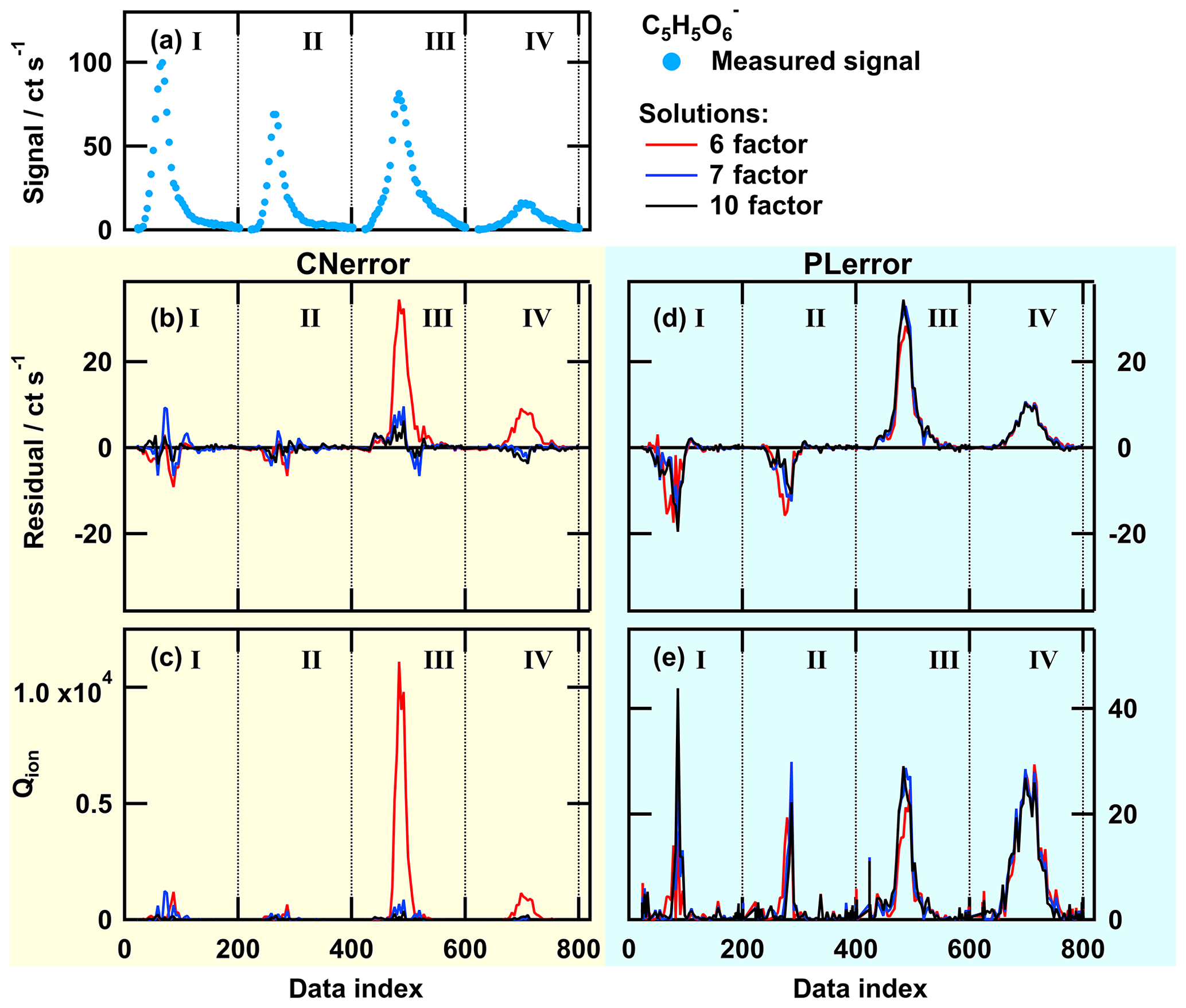
Figure A1 Single ion thermogram (a), residual (b, d), and Q_ion values (c, e) as time series for solutions with 6, 7, or 10 factors for PMF run with CNerror (b, c) and PLerror (d, e) for the ion ${\mathrm{C}}_{\mathrm{5}}{\mathrm{H}}_{\mathrm{5}}{\mathrm{O}}_{\mathrm{6}}^{-}$. The data set contains thermogram scans for high-O:C SOA particles for the following sampling conditions: dry – t_evap=0.25 h (I); dry – t_evap=4 (II); wet – t_evap=0.25 h (III); and wet – t_evap=4 h (IV). Note that the y scaling is the same in panels (b) and (d), but it is much smaller in (e) than in (c).

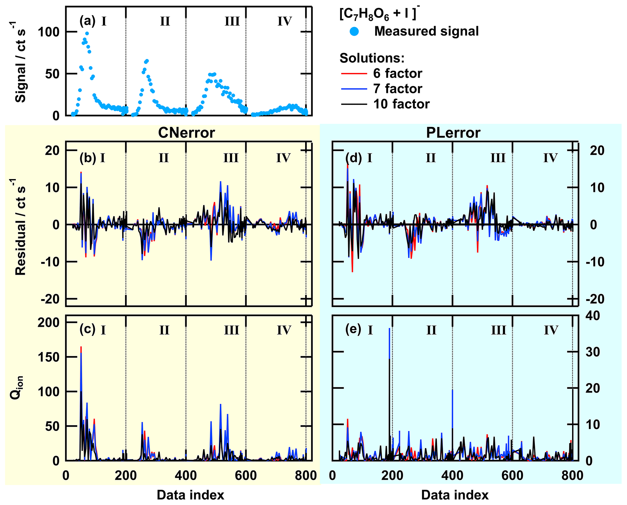
Figure A2 Single ion thermogram (a), residuals (b, d), and Q_ion values (c, e) as time series for solutions with 6, 7, or 10 factors for PMF run with CNerror (b, c) and PLerror (d, e) for the ion [C₇H₈O₆+I]⁻. The data set contains thermogram scans for high-O:C SOA particles for the following sampling conditions: dry – t_evap=0.25 h (I); dry – t_evap=4 h (II); wet – t_evap=0.25 h (III); and wet – t_evap=4 h (IV). Note that the y scaling in (e) is much smaller than in (c).

Figure A3 Combined single ion thermograms of the ion ${\mathrm{C}}_{\mathrm{5}}{\mathrm{H}}_{\mathrm{5}}{\mathrm{O}}_{\mathrm{6}}^{-}$ and PMF factor thermograms for 6- (a, c) and 7-factor (b, d) solutions. Left column values (a, b) are calculated with CNerror and right column values (c, d) are calculated with PLerror. The data set contains thermogram scans for high-O:C SOA particles for the following sampling conditions: dry – t_evap=0.25 h (I); dry – t_evap=4 h (II); wet – t_evap=0.25 h (III); and wet – t_evap=4 h (IV). Note that generally the factors are not the same between the two error schemes or the two solutions (i.e. F1 in the 6-factor solution with CNerror is different to F1 in the 7-factor solution with CNerror, etc.).

To illustrate why there is no further improvement in the PMF results with the PLerror scheme and to show at which part of the data set the error schemes create different results, we investigated the behaviour of the PMF solutions for individual ions. We selected two ions with similar signal strength and different error scheme responses. Both error schemes provided comparable PMF results for the ion [C₇H₈O₆+I]⁻ (Fig. A2) while the thermogram behaviour of the ion ${\mathrm{C}}_{\mathrm{5}}{\mathrm{H}}_{\mathrm{5}}{\mathrm{O}}_{\mathrm{6}}^{-}$ (Fig. A1) was not captured well with the PLerror scheme. Note that the latter represents the group that mostly contained ions that were affected by aqueous-phase chemistry. For the 6-factor solution (red line in Fig. A1b and d), the residual time series for this ion has similar values for thermogram scans III and IV in both error schemes, but increasing the number of factors by 1 seems to only have a noticeable effect in the case of the CNerror. This is because, in this case, the Q_ion values $(Q_{\mathrm{ion}}={\left(\frac{{\mathbf{E}}_{\mathrm{ion}}}{{\mathbf{S}}_{\mathrm{ion}}}\right)}^{\mathrm{2}})$ are extremely high for that part of the data set (red line in panel c). Investigating the Q_i values summed over all observations (mass spectra) shows that this ion (${\mathrm{C}}_{\mathrm{5}}{\mathrm{H}}_{\mathrm{5}}{\mathrm{O}}_{\mathrm{6}}^{-}$) has the fifth-highest contribution to overall Q∕Q_exp. The other ions with such a high single contribution to Q∕Q_exp exhibit very similar behaviour of their residuals and Q_ion values. Together, they account for 15 % of the overall Q∕Q_exp value in the 6-factor case. So, adding an additional factor to describe that portion of the data set will strongly decrease Q_ion and also Q∕Q_exp, which indicates a better fit. In the case of the PLerror, the Q_ion values exhibit very similar profiles for all four thermogram scans (Fig. A1d and e). Thus, changing any parameter for ${\mathrm{C}}_{\mathrm{5}}{\mathrm{H}}_{\mathrm{5}}{\mathrm{O}}_{\mathrm{6}}^{-}$ will have little effect on the Q_ion values and, therefore, on the overall Q∕Q_exp. This example clearly shows how the selection of the error values guides the focus of PMF, i.e. which part of the data set still needs improvement when the number of factors is increased. In Fig. A3, the contribution of each factor to the signal of ${\mathrm{C}}_{\mathrm{5}}{\mathrm{H}}_{\mathrm{5}}{\mathrm{O}}_{\mathrm{6}}^{-}$ is shown with coloured areas for the 6- (top) and 7-factor (bottom) solutions for CNerror (a and c) and PLerror (b and d) to highlight the changes caused by the increase of the number of factors for this ion. In addition to reducing the residual for the peaks in thermograms III and IV by using the CNerror, the additional factor substantially alters the factor time series for this ion and is therefore likely affecting our interpretation of these factors – presumably towards improved accuracy. Indeed, the “new” factor F3 was identified in Sect. 3.3 as HV3, which contains the products of the chemical reactions in the aqueous phase.

This error-scheme-dependent performance of PMF is not controlled by the signal strength of the ion or the ratio between signals of combined thermograms. The two example ions were explicitly chosen because of their similar signal strength in all thermograms (compare Figs. A1a and A2a). Instead, it seems that the PLerror does not assign enough weight to the peak region of the ion thermograms. Thus, it cannot resolve the changes in peak shape (i.e. the large shift towards higher desorption temperatures). As the shift is caused by specific processes in the particle phase, PMF with the PLerror will not identify these processes.

These two observations, the CNerror explaining more of the observed variance in general and capturing the complex chemical processes in the particles, lead us to the conclusion that the CNerror yields the more interpretable results for this study and data set and should be used – even though it is not the “true” measurement error of the data.

Appendix B: Mathematical symbols and notations used in the equations throughout the paper

Symbol	Explanation
X, Xij	Data matrix (n×m) and data matrix element
p	Number of factors
m	Number of observations (mass spectra) in the data set
n	Number of ions in the data set
G	Factorisation matrix containing the factor thermograms
	as columns (n×p)
F	Factorisation matrix containing the factor mass spectra
	as rows (p×m)
E, Eij	Residual matrix and residual matrix element
R, Rij	Reconstructed data matrix (R=GF) and reconstructed
	data matrix element
S, Sij	Measurement error matrix and error matrix element
absVartotal	Total absolute variance
absVarexp	Explained absolute variance
Ratioexp	Ratio of explained to total absolute variance
Q	Square of the residual scaled with the error summed
	over all ions and observations (mass spectra)
Qexp	Expected Q value, in the ideal case, with the “true”
	measurement error equal to n×m
Qj	Square of the residual scaled with the error summed
	over all observations (mass spectra)
Qi	Square of the residual scaled with the error
	summed over all ions
Qion	Square of the residual scaled with the error
	for a single ion as time series
Q∕Qexp	Optimisation parameter in PMF