Consumption of CH₃Cl, CH₃Br, and CH₃I and emission of CHCl₃, CHBr₃, and CH₂Br₂ from the forefield of a retreating Arctic glacier

The Arctic is one of the most rapidly warming regions of the Earth, with predicted temperature increases of 5–7 ^∘C and the accompanying extensive retreat of Arctic glacial systems by 2100. Retreating glaciers will reveal new land surfaces for microbial colonisation, ultimately succeeding to tundra over decades to centuries. An unexplored dimension to these changes is the impact upon the emission and consumption of halogenated organic compounds (halocarbons). Halocarbons are involved in several important atmospheric processes, including ozone destruction, and despite considerable research, uncertainties remain in the natural cycles of some of these compounds. Using flux chambers, we measured halocarbon fluxes across the glacier forefield (the area between the present-day position of a glacier's ice-front and that at the last glacial maximum) of a high-Arctic glacier in Svalbard, spanning recently exposed sediments (<10 years) to approximately 1950-year-old tundra. Forefield land surfaces were found to consume methyl chloride (CH₃Cl) and methyl bromide (CH₃Br), with both consumption and emission of methyl iodide (CH₃I) observed. Bromoform (CHBr₃) and dibromomethane (CH₂Br₂) have rarely been measured from terrestrial sources but were here found to be emitted across the forefield. Novel measurements conducted on terrestrial cyanobacterial mats covering relatively young surfaces showed similar measured fluxes to the oldest, vegetated tundra sites for CH₃Cl, CH₃Br, and CH₃I (which were consumed) and for CHCl₃ and CHBr₃ (which were emitted). Consumption rates of CH₃Cl and CH₃Br and emission rates of CHCl₃ from tundra and cyanobacterial mat sites were within the ranges reported from older and more established Arctic tundra elsewhere. Rough calculations showed total emissions and consumptions of these gases across the Arctic were small relative to other sources and sinks due to the small surface area represented by glacier forefields. We have demonstrated that glacier forefields can consume and emit halocarbons despite their young age and low soil development, particularly when cyanobacterial mats are present.

1 Introduction

Despite being present at only low concentrations in the atmosphere (parts per trillion, ppt), halocarbons play an important role in the destruction of ozone by supplying halogens to the stratosphere and the troposphere (Butler, 2000; Mellouki et al., 1992; Montzka et al., 2011). Methyl chloride (CH₃Cl) and methyl bromide (CH₃Br) are the most important natural sources of chlorine (16 %) and bromine (50 %) to the troposphere and are important contributors to stratospheric ozone loss (Carpenter et al., 2014). After CH₃Cl, chloroform (CHCl₃) is the next largest natural carrier of chlorine. Bromoform (CHBr₃) and dibromomethane (CH₂Br₂) are the most abundant short-lived brominated compounds and contribute ∼4 %–35 % of bromine to the stratosphere (Montzka et al., 2011). Methyl iodide (CH₃I) is the most important very-short-lived iodinated gas species in the atmosphere with a lifetime of ∼7 d (Montzka et al., 2011). Some of the aforementioned gases have anthropogenic sources, many of which have decreased in magnitude under the Montreal Protocol (Carpenter et al., 2014). This has increased the relative importance of the natural sources of these halocarbons. The contribution of halocarbons to atmospheric processes makes it important to fully constrain present-day sources and their likely change under future climate change scenarios.

Most natural sources of halocarbons involve biological processes driven by plants, algae, and fungi, with methyl halides (CH₃X; X= Cl, Br, I) generated as a by-product of methyltransferase activity and polyhalomethanes (e.g. CHCl₃, CHBr₃, CH₂Br₂) produced as a by-product of haloperoxidase activity (Manley, 2002). Marine biogenic sources are predominantly driven by macro- and micro-algae and are particularly important for CHBr₃ and CH₂Br₂ which are considered to be exclusively marine (Laturnus et al., 1998; Montzka et al., 2011; Sturges et al., 1993; Tokarczyk and Moore, 1994). The other halocarbons studied here (CH₃X, CHCl₃) also have a wide range of terrestrial biogenic sources, including tropical and temperate forests, temperate peatlands, and Arctic tundra (Farhan Ul Haque et al., 2017; Forczek et al., 2015; Rhew et al., 2008; Simmonds et al., 2010).

Although biological sources of halocarbons dominate, abiotic sources are also possible, including emissions from open oceans (Chuck et al., 2005; Stemmler et al., 2014), oxidation of soil organic matter, and degradation of leaf litter and plants (Derendorp et al., 2012; Keppler et al., 2000; Wishkerman et al., 2008). The major, non-atmospheric, natural sinks of the halocarbons are the oceans (primarily abiotic) and bacterial degradation in soils (Nadalig et al., 2014; Shorter et al., 1995; Ziska et al., 2013). The bacterial soil sink has been identified in wide-ranging habitats from temperate forests to the tundra (e.g. Khan et al., 2012; Teh et al., 2009). Despite this considerable research, uncertainties remain around the magnitudes of natural sources and sinks of halocarbons due in part to large variation around mean fluxes caused by spatial and temporal variability (e.g. Dimmer et al., 2001; Leedham et al., 2013; Montzka et al., 2011; Stemmler et al., 2014). Reduction of the uncertainties and increased understanding of the processes influencing natural halocarbon fluxes are important for predicting future change.

A previously unstudied environment for halocarbon fluxes is the young soil found on the forefields of retreating glaciers. As the Arctic warms, increasing areas of land are being exposed by ongoing glacial retreat, a process that is forecast to continue throughout the 21st century (ACIA, 2005; Graversen et al., 2008). The newly exposed sediment is colonised by microbes such as heterotrophic bacteria and fungi, CO₂- and nitrogen-fixing cyanobacteria, and nitrogen-fixing diazotrophs that fix nutrients into the developing soil (Bradley et al., 2014; McCann et al., 2016). Soil stabilisation on newly exposed glacier forefields (i.e. prior to widespread plant colonisation) is primarily driven by cyanobacterial colonisation and the subsequent formation of soil crusts (Hodkinson et al., 2003). Through nutrient-fixing and soil stabilisation processes, the microbial community enables the succession of higher plants, eventually leading to a tundra-type ecosystem for high-Arctic locations (e.g. Hodkinson et al., 2003; Moreau et al., 2008).

Despite the forecasting of enhanced glacial retreat, trace gas emissions from glacier forefields have not been well-investigated, with studies primarily focussing on CO₂ fluxes, particularly from higher plants on older surfaces, or CH₄ fluxes (Chiri et al., 2015; Muraoka et al., 2008). There have been no studies on halogenated trace gas fluxes from the forefield environment and how they might be affected by the accelerated change occurring in the Arctic. With the expansion of glacier forefields through increasing glacial retreat in the coming decades, understanding the processes occurring in these soils is timely. To investigate the impact of soil development and the associated microbial-to-plant succession on halogenated trace gas fluxes, we conducted in situ flux measurements of CH₃Cl, CH₃Br, CH₃I, CHCl₃, CHBr₃, and CH₂Br₂ at five sites spanning newly exposed soils (exposed <10 years ago) to established tundra (exposed approximately 1950 years ago) in front of a high-Arctic glacier.

2 Study site

2.1 General description of the location

Midtre Lovénbreen is a small (5.4 km²) valley glacier situated on the northern side of the Brøggerhalvøya Peninsula, in northwestern Svalbard ($\mathrm{78}{}^{\circ }{\mathrm{53}}^{\prime }$ N, $\mathrm{12}{}^{\circ }{\mathrm{04}}^{\prime }$ E). The glacier has been in near-constant negative mass balance since measurements began in 1968 and probably since at least the 1930s (Kohler et al., 2007). Warming mean annual temperatures since the 1920s have resulted in approximately 1.1 km of glacial retreat from a prominent moraine to its current position 1.8 km from the fjord edge (Fig. 1). Between 1966 and 1990, this retreat resulted in the exposure of 2.3 km² of land and is a process that continues today (Moreau et al., 2008). The exposed area is characterised by the dominance of large rock fragments (>5 cm diameter) and is influenced by glacial runoff with intermittent and shifting meltwater channels. The progression of the community assemblages along the glacier forefield chronosequence has occurred at slower rates than are typical, with cyanobacterial crust and lichens still prevalent beyond 150 years of exposure (Hodkinson et al., 2003). Vascular plants and bryophytes are present sporadically and increasingly with exposure age. The area experiences a maritime polar climate. The mean air temperature at the weather station in nearby Ny-Ålesund in July 2017, when this study was undertaken, was 6.1 ^∘C (Norway MET, 2017). Mean summer soil temperatures (∼2 mm below surface) on the forefield have been measured at 7–9 ^∘C (Hodkinson et al., 2003).

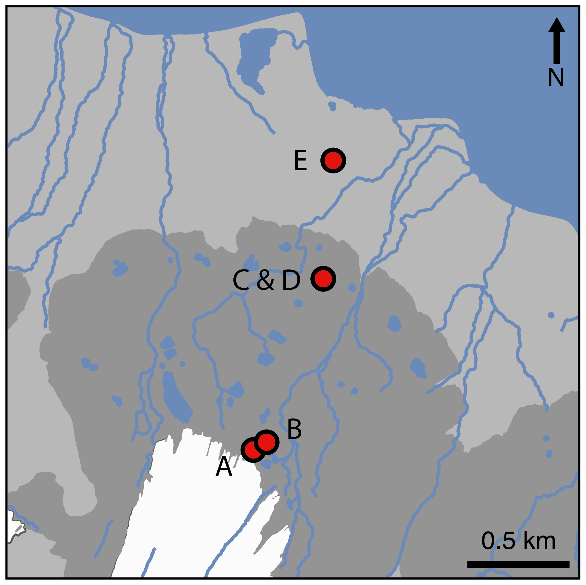
Figure 1 Locations of snout (A), pond mat (B), disturbed mat (C), established mat (D), and tundra (E) sites on the forefield of Midtre Lovénbreen glacier (white). The moraine field is denoted in dark grey, the maximum extent of which marks the furthest extent of the glacier during the Little Ice Age. Data used to create the base map are from Norwegian Polar Institute (2014).

2.2 Specific descriptions of the sites

Five different land surface types were studied in four different locations along a transect between the glacial snout and the fjord (Fig. 1). The sites had different vegetation types and coverage (Fig. 2). The exposure ages of the sites (in years before 2017) were estimated from dates obtained by ¹⁴C dating and aerial photography in other studies (Hodkinson et al., 2003; Moreau et al., 2008). The site nearest the glacier's snout (snout site) had an exposure age of approximately 5 years and was characterised by bare sediment, with little to no visible signs of life (Fig. 2a). Approximately 100 m from the glacier's snout, the second site (pond mat site) was located on the margins of a dried-up (by July) snowmelt pond in a small depression between the moraines. Around the margins of the pond, cyanobacterial mats had begun to form (Fig. 2b). The surrounding moraines were still largely barren. The pond mat site is estimated to have been exposed for around 20 years. The third and fourth sites were located near the middle of the transect on an expanse of relatively flat land behind (∼ south) the prominent Little Ice Age moraine (Fig. 1). The established mat site was located on the extensive cyanobacterial mats which cover large expanses of the flatter land (Fig. 2d). A site immediately adjacent to the mats where the mats had been disturbed by snowmelt flowing from ponds (disturbed mat site) was also studied as a direct comparison (Fig. 2c). The exposure age of the established mat and disturbed mat sites was estimated at 100 years. The final site (tundra site) was located about 200 m from the coast (Fig. 2e). At this site, small bluffs of limestone and siltstone provided some shelter from the shifting nature of the glacial runoff rivers which otherwise hamper colonisation of much of the floodplain between the moraines and the fjord. The tundra site had a soil depth of about 15 cm and 100 % vegetation coverage. Dominant species included Bryophyta spp. and Carex rupestris, Salix polaris, and Racomitrium lanuginosum. Radiocarbon dating near the tundra site (∼70 m west) has provided a date of exposure of 1850–1926 BP (before present, defined as 1 January 1950 by the radiocarbon age scale; Hodkinson et al., 2003). This is equivalent to 1917–1993 years older (or approximately 1950 years) than the year of analysis (2017).

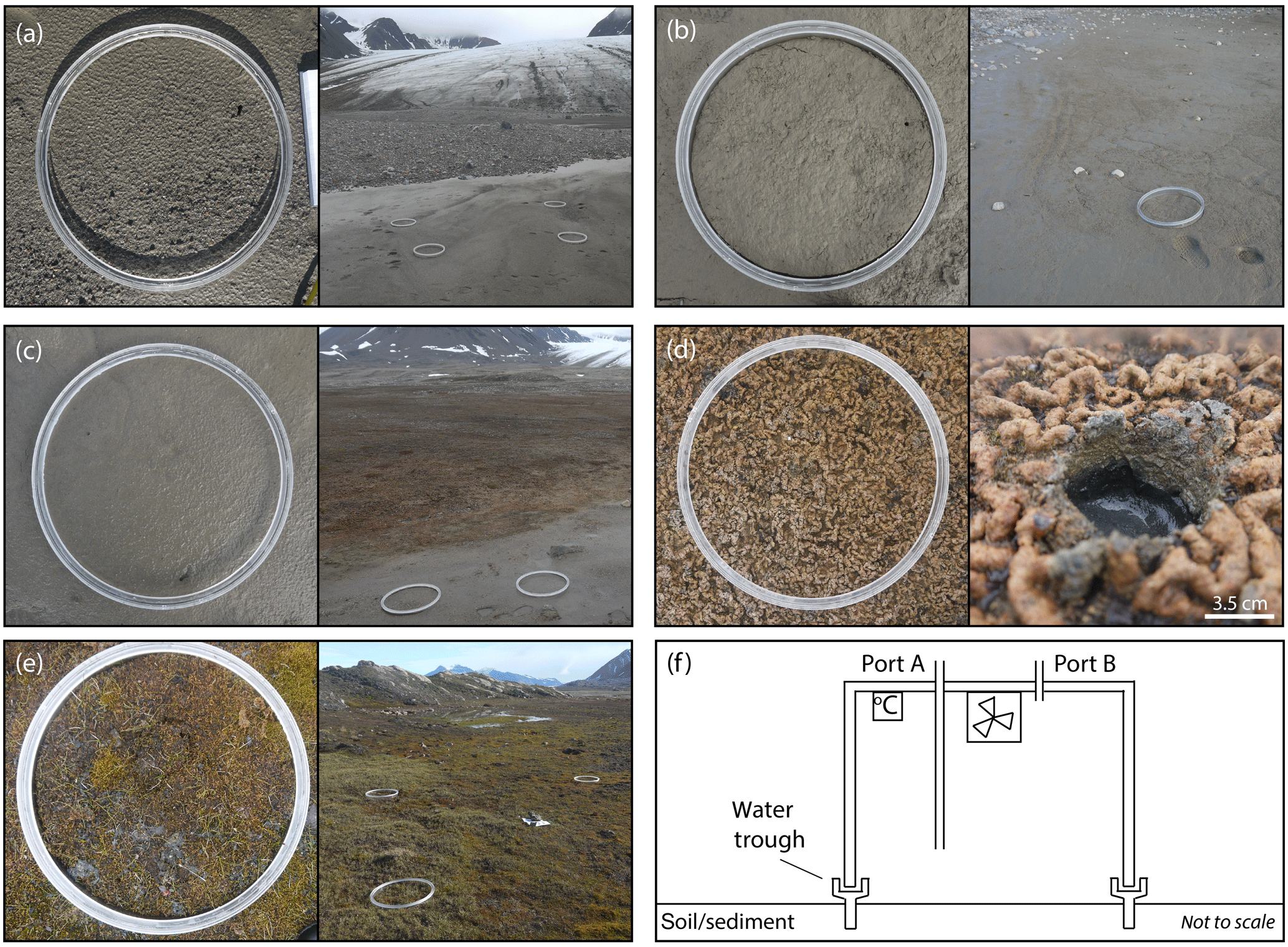
Figure 2 The visible differences in land surface type and colonising species at the snout (a), pond mat (b), disturbed mat (c), established mat (d), and tundra (e) sites and a schematic diagram of the flux chamber's design showing sampling ports, fan, and temperature logger (f). The width of the chamber collar in (a)–(e) is 0.39 m.

3 Methods

3.1 Flux experiments

Four custom-made, cylindrical, Perspex flux chambers (0.029 m³) composed of a collar (0.07 m height) and top (0.22 m height, Fig. 2f) were deployed for gas analysis between 25 and 31 July 2017. Preliminary experiments were conducted near the established mat site in 2016 to determine the impact on gas fluxes of covering the chambers with a reflective material so that the experiments were conducted in the dark. The tests showed no statistical difference (two-sample t test; Sect. 3.5) between covered and uncovered chambers (conducted in duplicates) for mean fluxes of CH₃Cl, CH₃Br, and CH₃I (Fig. 3; other halocarbons not analysed; experiment conducted over 5 h). Despite there being no statistical difference in gas concentration change, the covered chambers were used for the main experiments in 2017 to prevent overheating when in direct sunlight, therefore minimising the influence of heat on the soil processes involved in the fluxes. The collar was embedded in the sediment surface prior to sampling (at least 18 h) to allow gases released or absorbed from breaking the surface to equilibrate with the background air concentrations. At the tundra site, where plant roots were abundant, a small knife was used to cut through the roots as the collar alone could not break through the surface. An integrated “trough” on the collar was filled with deionised water (14–18 MΩ cm) to provide a leak-tight seal with the upper section of the chamber (Fig. 2f). A fan (24 m³ h⁻¹; San Ace 60) was operated continuously during incubation to ensure the chamber air remained mixed. Tinytag temperature loggers (Gemini data loggers) were fixed to the underside of the chamber lid.

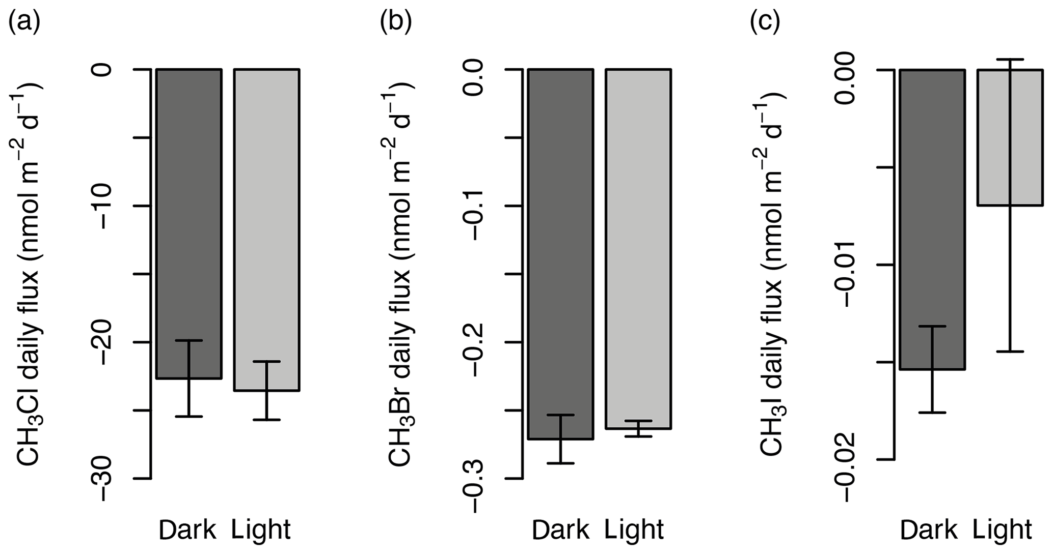
Figure 3 Comparison of the gas flux (nmol m⁻² d⁻¹) in un-darkened (light) and darkened (dark) chambers for CH₃Cl (a), CH₃Br (b), and CH₃I (c) from preliminary experiments in 2016. Error bars show the standard deviation.

Two sampling ports, constructed from polypropylene BSP fittings, Luer-lock stopcocks, and 20 cm polypropylene tubing (port A only, Fig. 2f), enabled gas sampling to be conducted 1 and 2 h after sealing the chamber. Two types of gas sampling were conducted; first, 3.7 mL samples were taken for CO₂ and CH₄ analysis in the laboratory in Bristol, UK; second, 2.5 L samples were taken for halocarbon analysis with a gas chromatograph–mass spectrometer (GCMS) at the UK station in Svalbard. Sampling was conducted with four replicates (four chambers). Each site was analysed on a different day, with the snout and pond mat sites analysed once (four replicates) and the established mat, disturbed mat, and tundra sites analysed twice (2 separate days of four replicates each, total of eight replicates). Chambers and collars were washed with deionised water and dried with paper towels between sites to minimise contamination.

Both a laboratory and a field blank test of the flux chamber equipment were conducted by placing the chambers onto aluminium-foil trays and filling the inside of the chamber collar with a 1 cm deep layer of deionised water to create a seal. For the field blank tests, the aluminium-foil trays were placed on wooden boards (to provide a flat surface) on the ground close to the tundra site. The blank tests were conducted with four replicates and gases were measured as in Sect. 3.2 and 3.3.

3.2 CO₂ and CH₄ sampling and analysis

CO₂ and CH₄ were sampled in duplicate at each time point using a glass gas-tight syringe (Hamilton). Samples were taken from the ambient air (time 0) and from the chamber headspace via port B (Fig. 2f, times 1 and 2). A total of 5.5 mL of air was drawn through the tap using the syringe and flushed to ambient prior to withdrawing a further 5.5 mL of sample into the syringe. A total of 1.5 mL of the sample was used to flush a syringe filter (0.2 µm) and needle. The remaining 4 mL of sample was aseptically injected into a 3.7 mL evacuated vial (Exetainer^®; Labco) via the flushed 0.2 µm syringe filter. Exetainers were stored (within 4 h of sampling) and transported at +4 ^∘C until analysis in the UK within 36 d. Exetainers have previously been shown to be suitable for storage of CO₂ and CH₄ for at least 28 d, but not as long as 84 d (Faust and Liebig, 2018), and therefore we consider the storage time of up to 36 d to have had minimal impact on the measured concentrations.

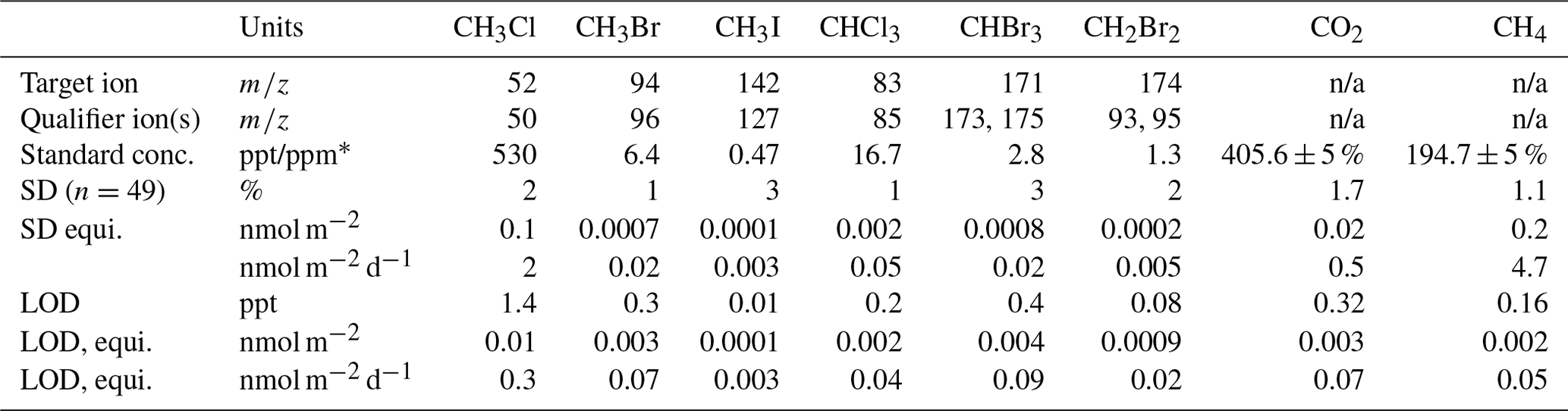
Exetainer samples were injected into an Agilent 7890A gas chromatograph (GC) fitted with a methaniser (at 395 ^∘C) and an FID (flame-ionising detector, at 300 ^∘C). Separation of methane (CH₄) and carbon dioxide (CO₂) was achieved using a molecular sieve 5A, 60–80 mesh, 8 ft $\times \mathrm{1}/\mathrm{8}$ in. column, held at 30 ^∘C for 4 min, before being ramped at 50 ^∘C min⁻¹ to 180 ^∘C. Calibration standards (mixed air, BOC) were run twice daily. The percentage variance, limit of quantification, and limit of detection for each gas are displayed in Table 1. Concentrations of the samples were calculated from a linear regression line (r>0.99, n=5) of manual dilutions of certified (±5 %) standards with 5.0-grade Argon (BOC) fitted with an in-line gas desiccator. The ideal gas law was used to convert gas concentrations to molar amounts which were then corrected for dilution.

Table 1 The standard concentration, limit of quantification (standard deviation, SD), and limit of detection (LOD) for each gas analysed, with the target ion and qualifier ion(s) (m∕z; mass/charge) shown for gases analysed by a GCMS. ^* The units are parts per trillion for the halocarbons and parts per million for CO₂ and CH₄. n/a – not applicable to the method of measurement. “equi.” is short for equivalent.

3.3 Halocarbon sampling and analysis

The 2.5 L air samples for the analysis of halocarbons were taken using a small pump (SKC, Twin Port Pocket Pump) at 250 mL min⁻¹ into 3 L Tedlar gas-tight bags (polypropylene fittings, SKC). All sample bags were flushed three times with 5.0-grade synthetic zero air (dry and CO₂-free) prior to use, with laboratory testing indicating this removed any background contamination. The length of sampling time (10 min) required the chambers to be sealed approximately 12 min apart to allow time for sampling. A sample of ambient air was taken between the sealing of the first and second chambers and again between the sealing of the third and fourth chambers. An average of the mixing ratios of the two ambient measurements was used as time 0 for the four chambers. Headspace analysis of each chamber was taken after 1 and 2 h through the extended tubing of port A to further ensure mixing of the chamber air (Fig. 2f). A 3 L sample bag flushed and filled with the synthetic air was connected to port B during sampling to maintain ambient pressure within the chamber and prevent air being drawn through the soil. A total of 50 mL of chamber air was flushed through the port A tubing and the pump prior to taking the 2.5 L sample. Sample bags were kept in the dark until analysis (within <20 h) at the UK station in Ny-Ålesund. Tests conducted on the sample bags found detectable but small changes in gas concentrations 20 h after being flushed with the standard (+0.002 nmol CH₃Cl, −0.00001 nmol CH₃Br, +0.00001 nmol CH₃I, +0.001 nmol CHCl₃, +0.00002 nmol CHBr₃, +0.00001 nmol CH₂Br₂; concentrations converted to moles per sample bag using the ideal gas law).

Analysis of halocarbons with part-per-trillion (ppt) atmospheric concentrations was conducted with a custom-built adsorption–desorption system (ADS; developed by the University of Bristol; Simmonds et al., 1995) connected to an automated gas chromatograph–mass spectrometer (GCMS). A total of 1.5 L of whole-air sample was drawn through a Nafion permeation drier (continuous counter-purge of dry 5.0-ultra-grade synthetic air at 170 mL min⁻¹) before being condensed onto an absorbent filled microtrap held at −50 ^∘C using electrical resistance (Peltier device). The concentrated sample was desorbed by raising the microtrap to 240 ^∘C using direct ohmic heating. The sample was carried through a fused silica transfer line (100 ^∘C) by 5.0-grade helium, purified by a Universal Trap, into a Hewlett Packard 6890A gas chromatograph. Separation of methyl chloride (CH₃Cl), methyl bromide (CH₃Br), methyl iodide (CH₃I), dibromomethane (CH₂Br₂), chloroform (CHCl₃), and bromoform (CHBr₃) was achieved using a 25 m capillary GC column (Varian, PoraBOND Q, 320 µm i.d., 5 µm film thickness) which was held at 40 ^∘C for 3 min, ramped at 22 ^∘C min⁻¹ to 84 ^∘C and held for 1 min, then ramped at 22 ^∘C min⁻¹ to 250 ^∘C where it was held for 37.73 min (total time: 49 min). Samples were identified from their fragmentation spectra using a Hewlett Packard 5973 mass spectrometer detector (quadrupole at 150 ^∘C, source at 230 ^∘C) scanning for selected ion masses (Table 1). Bromochloromethane (CH₂BrCl) and diiodomethane (CH₂I₂) were also scanned for (target ions of 128 and 268, respectively; qualifier ions of 130 and 141, respectively). CH₂BrCl was present in only trace amounts in the standard (below the limit of detection) and was thus not quantifiable. CH₂BrCl is discussed in this paper based on relative changes to the peak area. CH₂I₂ was not present in the standard. This is likely due to its exceptionally short atmospheric lifetime (0.003 d; Law et al., 2006), meaning its highly unlikely to persist in the ambient atmosphere, from which the standard was made. CH₂I₂ was not detected during the experiments either, which follows with previous research that has only identified its production in marine environments, particularly by macroalgae and sea ice microalgae (Carpenter et al., 2000, 2007).

Quantification of compounds was determined using GCWerks software (http://gcwerks.com, last access: 14 November 2018) from the average peak area of the two closest standard analyses, which were run every second sample. The standard was cryo-filled from the ambient air on 11 January 2017 at the Norwegian Zeppelin Observatory (operated by the Norwegian Institute for Air Research, NILU), 2 km south of Ny-Ålesund at 475 m a.s.l. on Zeppelin Mountain. The standard was calibrated on the Zeppelin Medusa (part of the Advanced Global Atmospheric Gases Experiment (AGAGE; Prinn et al., 2018)) using tertiary standards linked to the primary standards prepared at Scripps Institution of Oceanography (SIO) for CH₃Cl and CH₃Br (SIO-05 calibration scale), and for CHCl₃ (SIO-98 calibration scale). CH₃I, CHBr₃, and CH₂Br₂ are calibrated via AGAGE tank comparisons carried out in Boulder, Colorado, against National Oceanic and Atmospheric Administration (NOAA) calibration scales (CH₃I, NOAA-2004; CHBr₃, NOAA-2003; CH₂Br₂, NOAA-2003) using SIO tanks T-005B, T-009B, and T-102B. Due to the increased number of steps to transfer these calibration scales, flux calculations for these three species have an additional error associated with them. The detection limit (3 times the baseline noise), limit of quantification (variance), and standard concentration for each halocarbon are displayed in Table 1. The ideal gas law was used to convert gas concentrations to molar amounts. The dilution from the synthetic air bag used to maintain ambient pressure during sampling was corrected for by accounting for the moles of gas removed during sampling at each time point. The results are presented as daily fluxes in nanomoles per metre squared of land surface per day (nmol m⁻² d⁻¹). Daily fluxes were calculated from the change in the number of moles of gas present in the headspace over the first hour of the experiment, corrected for the mean change in moles during the first hour of the field blank tests. These mean blank changes were +0.2 nmol CH₃Cl m⁻², +0.01 nmol CH₃Br m⁻², +0.003 nmol CH₃I m⁻², −0.03 nmol CHCl₃ m⁻², −0.01 nmol CHBr₃ m⁻², and −0.002 nmol CH₂Br₂ m⁻². Mean daily fluxes are presented ±1 standard deviation. The daily fluxes were calculated from the change in moles in 1 h because the majority of the 2 h total change occurred within the first hour. For example, 78 % to 90 % of the initial moles of CH₃Cl and CH₃Br present in the chamber were consumed within the first hour at the established mat and tundra sites, with only 0.01 % to 4 % of additional consumption in the second hour. For the gases that were emitted, a similar pattern emerged where the proportion of gas emitted in the first hour of the total amount of gas emitted over the 2 h experiment was an average of 59 % of CHCl₃, 61 % of CHBr₃, and 60 % of CH₂Br₂ at the established mat and tundra sites. Presumably the slowdown in the rate of change after 1 h was due to reactants being consumed from the air trapped inside the chamber. Because of this, we advocate that our daily flux rates (nmol m⁻² d⁻¹) are a minimum estimate.

3.4 Physical, chemical, and biological sampling and analysis

3.4.1 In-field measurements and sampling

The internal chamber temperature was recorded at 5 min intervals (Tinytag loggers; Gemini), and an average was calculated for the 2 h duration of each experiment. At the end of the incubation, the chamber tops were carefully removed without disturbing the sediment surface. Aliquots of sediment (∼1 g) from the centre of each collar were taken aseptically using 15 mL sterile falcon tubes. These samples were frozen at −20 ^∘C within 4.5 h of sampling and were transported and stored at this temperature until analysis of cell numbers in Bristol within 55 d or less.

After the sterile samples were conducted, a soil moisture sensor (ML3 ThetaProbe, accuracy of ±1 %) was used to measure the volumetric water content of the sediment in each quarter (0.03 m²) of the chamber. Small cores (∼4 cm deep) of the sediment were taken from the centre of two opposite quarters of the chambers' footprint. The cored samples were broken up and dried for 20 h at 60 ^∘C prior to transport to the UK for soil texture, total carbon (TC) content, total nitrogen (TN) content, and organic matter (OM) content analyses

In the centre of each chamber, a corer was used to determine the depth of the water table. In some cases the water table could not be reached due to the presence of high numbers of large (>5 cm diameter) rocks in the near subsurface which were not practical to dig through.

3.4.2 Organic matter, total nitrogen, total carbon, and soil texture

Prior to OM, TC, and TN content and soil texture analyses, plant roots (present at the tundra site) and pieces of cyanobacterial mat (present at the established mat site) were removed with tweezers from the dried samples. Additionally, a sieve was used to remove small roots (>2 mm) from the tundra site samples but it was not possible to remove roots smaller than this.

Samples for OM, TC, and TN content analyses were re-dried at 105 ^∘C for 19 h to ensure removal of water. Approximately 4 g of a known weight of the dried sample from each quarter-chamber core was then furnaced at 450 ^∘C for 5 h to determine the OM content (weight %) by mass loss on ignition. The larger weight of sample used here meant that some very small roots were likely present in these samples and may inflate the values. In comparison, TC and TN content was analysed on less than 20 mg of sample, meaning no root matter was likely to be present.

An elemental analyser 1110 fitted with a TCD (temperature-controlled detector) was used to measure percentage weight of TC and TN in an 8 to 19 mg, <250 µm, well-mixed aliquot of the re-dried core sample by flash heating to 1000 ^∘C. TC and TN contents were quantified using a certified aspartic acid standard containing 36.14 % C and 10.49 % N. This method has a limit of detection (LOD) of 0.01 % for both TC and TN and a precision of 0.06 % for TC and 0.01 % for TN (n=6) as determined from a soil standard containing 2.29 % TC and 0.21 % TN.

To determine the heterogeneity and average size of grains at each site, the remaining approximately 10 g of re-dried core sample was sieved to determine the percentage weight of the sample with grain sizes greater and smaller than 2 mm.

3.4.3 Bacterial abundance

Counts of bacteria were conducted after methodology detailed by Bradley et al. (2016). Briefly, upon analysis, the samples were defrosted and 100 mg subsampled into sterile microcentrifuge tubes (1.5 mL, Eppendorf). The sample was diluted with 932 µL of Milli-Q (MQ) water (0.2 µm filtered) and fixed in 68 µL of 0.2 µm filtered 37 % formaldehyde (final concentration of 2.5 %). Samples were vortexed for 10 s and sonicated for 1 min at 30 ^∘C to disaggregate soil particles and separate the cells from them. The sample was then vortexed for 3 s with 10 µL of fluorochrome DAPI (4',6-diamidino-2 phenylindole) prior to being incubated for 10 min in the dark. The stained sample was vortexed for 10 s, and 100 µL of this was filtered through a black polycarbonate filter paper (0.2 µm pore size, 25 mm diameter) and then rinsed with 250 µL of MQ water (0.2 µm filtered). Bacterial cells were counted under UV light at 1000× magnification using an Olympus BX41 microscope. MQ water (0.2 µm filtered) was used to wash the filtering apparatus between each sample. Blank controls, to which no soil or sediment was added, were dispersed throughout the samples. Ten random grids (each 10³ µm²) were counted per sample. The number of cells per gram of wet weight sample was calculated. Cell numbers for the blank controls were below 50 cells mL⁻¹.

3.5 Statistical analysis

Differences between mean halocarbon fluxes from different sites were determined at the 95 % confidence level (p values <0.05) using pair-wise Welch two-sample t tests conducted in R (version 3.02.1, 2015). Correlations between halocarbon fluxes and the physical, chemical, and biological variables are estimated and presented using the “corrplot” package in R (Wei and Simko, 2017). An average value per chamber was calculated for the physical and chemical variables where multiple analyses were conducted at each chamber (OM, TC, TN, and texture; n=2). Matrices were produced from the data for all sites combined and from the data for three individual sites: disturbed mat, established mat, and tundra. The individual site matrices were generated because of the disparity in land surface “type” between sites, which results in large variation in physical, chemical, and biological variables. Bacterial cell numbers were excluded as a variable for the “within-site” correlation matrices because the four measurements conducted per site were deemed too few to be included in the analysis. Similarly, matrices were not produced for the snout and pond mat sites which only had four halocarbon flux data points each.

3.6 Calculation of regional fluxes

3.6.1 Calculation of total glacier forefield fluxes in the Arctic

To determine if halocarbon fluxes from glacier forefields were important regionally, we calculated an Arctic forefield total flux. First, we assumed an averaged flux for each halocarbon across the Midtre Lovénbreen forefield by subdividing the land surface into thirds. The first third is represented by fluxes from the snout and pond mat sites, the middle by fluxes from the disturbed and established mat sites, and the final third by fluxes from the tundra site. This gave an average forefield flux of −62 nmol CH₃Cl m⁻² d⁻¹, −1.0 nmol CH₃Br m⁻² d⁻¹, −0.04 nmol CH₃I m⁻² d⁻¹, 56 nmol CHCl₃ m⁻² d⁻¹, 0.5 nmol CHBr₃ m⁻² d⁻¹, and 0.4 nmol CH₂Br₂ m⁻² d⁻¹. The total area of glacier forefields across the Arctic has not been measured. Therefore, we assume that the size of Midtre Lovénbreen's forefield (2.7×10⁶ m²) is representative and combine this area with an estimated 9996 land-terminating glaciers (minimum elevation >50 m a.s.l.) located above 60^∘ N (WGMS, 2012), to calculate a total Arctic forefield land surface area of 2.7×10¹⁰ m². The estimated Arctic forefield land surface area was combined with the average forefield halocarbon fluxes and an assumed growing season of 100 d (with negligible fluxes out with this time) to calculate the regional source and sink of each halocarbon in moles and tonnes per year. The growing season length of 100 d was determined as the approximate average number of days with no ground snow cover (as determined by others, e.g. Bekku et al., 2003) measured at Ny-Ålesund weather station from 2009 to 2017 (102±26 d; Gjelten, 2018). We assume that the net flux of all gases is zero when outside of the growing season due to snow cover, low light (including no light during polar night), and low temperatures which would inhibit or reduce the rate of consumption or production processes in the soils to negligible or near-negligible rates. This would follow results from studies on other gas fluxes from soils during winter, e.g. CO₂ consumption was determined to be 1–2 orders of magnitude lower in winter than in summer in Alaskan tundra (Welker et al., 2000). However, the confirmation of halocarbon fluxes outside of the growing season cannot be definitively determined without further field studies.

3.6.2 Calculation of Arctic tundra fluxes

For the halocarbons (CHBr₃ and CH₂Br₂) that have not been measured on tundra before, we calculate an Arctic tundra flux based on calculations by Rhew et al. (2007) as follows. We assume that the growing season lasts 100 d (with negligible fluxes out with this time; see Sect. 3.6.1) and that the area of the Arctic tundra is 7.3×10¹² m² (Matthews, 1983). By assuming our tundra site fluxes are broadly representative of tundra as a whole, the average fluxes of CH₂Br₂ and CHBr₃ measured at the tundra site in nanomoles per square metre per day are combined with the Arctic tundra area and growing season length to calculate an annual Arctic flux in moles of gas per year, which was converted to gigagrammes of gas per year.

4 Results

4.1 Physical, chemical, and biological differences between sites

The environmental context for the halocarbon fluxes measured here was provided by the inter- and intra-site variation in the following physical, chemical, and biological parameters (Fig. 4). Volumetric water content and water table depth both varied between and within sites with the highest water content at the tundra site (50 % v∕v) but the shallowest water tables at the disturbed mat site (Fig. 4a–b). The texture of the sediment in the top 5 cm at the sites illustrated the heterogeneity of the moraine and fluvial outwash landscape, with near 100 % of grains <2 mm in diameter representing low-energy and sheltered environments at the tundra and pond mat sites compared to more variation at the other three sites (Fig. 4c).

Figure 4 Variation at each site of soil water content (a), water table depth (b), weight % of grains <2 mm diameter (c), organic matter content (d), total carbon content (e), total nitrogen content (f), bacterial cell numbers (g), CO₂ flux (h), and CH₄ flux (i). Horizontal black bar represents the median, red diamonds the mean for each site, and open circles the outliers. “dist. mat” is the disturbed mat site; “est. mat” is the established mat site. Water table was not measurable for the pond mat site due to rocky ground.

The chemical and biological parameters describe the increasing soil development with distance from the glacier's snout and therefore with exposure age. For example, bacterial cell abundances increased with distance from the glacier's snout, with the highest mean abundances at the established mat and tundra sites of 3.2×10⁸ cells g⁻¹ of sediment, compared with 0.6×10⁸ cells g⁻¹ of sediment at the snout site (Fig. 4g). The highest soil contents of OM, TC, and TN were all measured at the tundra site (Fig. 4d–f). Net emission of CO₂ was seen at the pond mat, established mat, and tundra sites, with fluxes spanning zero at the snout and disturbed mat sites. CH₄ emission was highest at the pond mat site with some consumption measured at the tundra site.

4.2 Halocarbon fluxes

The behaviour of the halocarbons over each surface type is broadly dictated by the compound type: mono-halogenated compounds (CH₃Cl, CH₃Br, CH₃I) were either consumed or fluctuated around zero, whereas polyhalomethanes (CHBr₃, CHCl₃, CH₂Br₂) were emitted from all surfaces (Fig. 5). The mono-halogenated compounds were strongly and consistently drawn down at the established mat and tundra sites with mean fluxes of $-\mathrm{106}\pm \mathrm{7}$ and $-\mathrm{126}\pm \mathrm{4}$ nmol m⁻² d⁻¹ respectively for CH₃Cl, $-\mathrm{1.7}\pm \mathrm{0.1}$ and $-\mathrm{1.8}\pm \mathrm{0.04}$ nmol m⁻² d⁻¹ respectively for CH₃Br, and $-\mathrm{0.10}\pm \mathrm{0.03}$ and $-\mathrm{0.13}\pm \mathrm{0.03}$ nmol m⁻² d⁻¹ respectively for CH₃I. A minor drawdown of CH₃Cl ($-\mathrm{11}\pm \mathrm{5}$ nmol m⁻² d⁻¹) and CH₃Br ($-\mathrm{0.3}\pm \mathrm{0.1}$ nmol m⁻² d⁻¹) occurred at the pond mat site, with near-zero fluxes at the snout site. Large variations in CH₃I were recorded at the snout, pond mat, and disturbed mat sites.

Figure 5 Daily fluxes (nmol m⁻² d⁻¹) at each site of CH₃Cl (a), CH₃Br (b), CH₃I (c), CHCl₃ (d), CHBr₃ (e), and CH₂Br₂ (f). Red diamonds represent the mean flux for each site. “dist. mat” is the disturbed mat site; “est. mat” is the established mat site.

The polyhalomethanes were emitted from all surfaces, although the emission was relatively small at the snout site. For CHCl₃, the site with the highest mean flux of 105±42 nmol m⁻² d⁻¹ was the established mat site. However, due to the variation in CHCl₃ fluxes, this was not statistically different from the mean tundra flux of 74±33 nmol m⁻² d⁻¹ (p value =0.1). Fluxes of CHBr₃ were similarly varied, with the highest mean emission from the disturbed mat site of 0.7±0.3 nmol m⁻² d⁻¹ being statistically similar to the flux at the tundra site of 0.6±0.1 nmol m⁻² d⁻¹ (p value =0.6). The highest mean flux of CH₂Br₂ was from the tundra site (0.8±0.3 nmol m⁻² d⁻¹), with a smaller mean flux at the established mat, disturbed mat, and pond mat sites (all three had a mean flux of 0.2 nmol m⁻² d⁻¹). CH₂BrCl was unquantified (Sect. 3.3) but was found to be emitted from all sites at similar relative magnitudes.

4.3 Relationships between halocarbon fluxes and physical, chemical, and biological variables

To understand the different physical, chemical, and biological factors associated with the halocarbon fluxes, correlations between them are presented in Fig. 6. Some of the chemical, physical, and biological variables were strongly related to site location because the five sites differed in key factors such as vegetation cover and type. For example, OM, TN, and TC contents were considerably higher at the tundra site than the other sites (Fig. 4d–f). Some halocarbon fluxes also showed site-dependent variation such as the strong consumption of CH₃Cl and CH₃Br at the established mat and tundra sites compared to minor drawdown at the other sites. Because of the differences in physical variables and halocarbon fluxes at each site, we calculated correlation matrices for the disturbed mat, established mat, and tundra sites separately (Fig. 6b–d). The difference between the correlations across all sites (Fig. 6a) compared with the correlations at individual sites (Fig. 6b–d) showed that relationships between the different variables are not always consistent across sites.

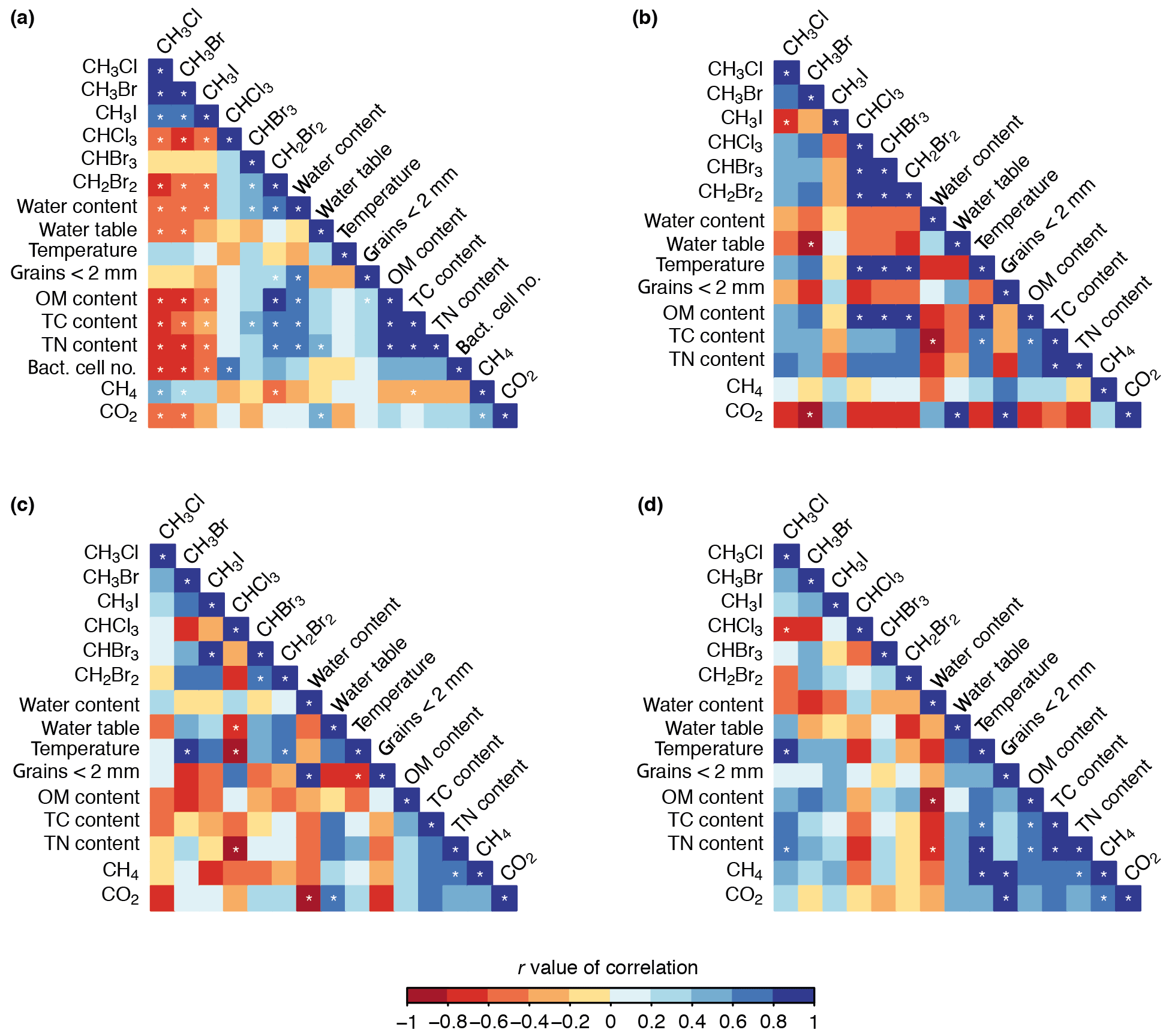
Figure 6 Correlations between halocarbon fluxes and the chemical, physical, and biological variables across all sites (a), the disturbed mat site (b), the established mat site (c), and the tundra site (d). White stars indicate correlations with 95 % confidence (p<0.05).

4.3.1 Halocarbon inter-correlations

The two groups of halocarbons, the methyl halides (CH₃Cl, CH₃Br, CH₃I) and the polyhalomethanes (CHBr₃, CHCl₃, CH₂Br₂), show similar patterns of correlation (Fig. 6a). The methyl halides were all positively correlated with each other (r>0.62, p<0.05), as were the polyhalomethanes, but more weakly (r>0.54; correlations with CHCl₃ were not significant, p>0.05). All correlations between the two groups were negative ($-\mathrm{0.18}<r<-\mathrm{0.62}$; insignificant for CHBr₃ due to the weakness of the correlation; $\mathrm{0}>r>-\mathrm{0.2}$, p>0.05). The negative correlation between the two groups indicated that, broadly, increased consumption of mono-halogenated compounds (i.e. more negative fluxes) correlated with increased production of poly-halogenated compounds.

The relationships within and between these two groups (methyl halides and polyhalomethanes) did not always persist across the three individual site analyses. For example, at the disturbed mat site, all the halocarbons except CH₃I were positively correlated (Fig. 6b), suggesting higher emission of the polyhalomethanes occurred with lower consumption of CH₃Cl and CH₃Br, contrary to the all-site relationship. Furthermore, there were instances where correlations across all sites appeared to be driven by the large size of their relationship at one site. For example, the weak positive correlation across all sites between the haloforms (CHX₃; X= Cl, Br), CHBr₃ and CHCl₃ (r=0.29), was inflated by their strong positive correlation at the disturbed mat site (r=0.98) which masked their negative correlation at the established mat and tundra sites ($r=-\mathrm{0.29}$ and −0.57, respectively). The results from the individual site analyses demonstrate the importance of investigating differences in halocarbon patterns by small-scale geography.

4.3.2 Correlations of methyl halides and chemical, physical, and biological variables

Across all sites, the mono-halogenated compounds were negatively correlated with OM, TC, TN, and bacterial cell numbers with the strongest correlation for CH₃Cl ($r<-\mathrm{0.60}$) and weakest for CH₃I ($r<-\mathrm{0.39}$), indicating greater methyl halide consumption (i.e. more negative fluxes) occurred with higher concentrations of OM, TC, TN, and bacterial cells in the sediment/soil. This was largely driven by high methyl halide consumption at the established mat and tundra sites where OM, TC, TN, and bacterial cell contents were highest. The relationship broadly persisted at the established mat site (Fig. 6c), but not at the disturbed mat and tundra sites (Fig. 6b, d). Across all sites, the methyl halides were negatively correlated with water content and water table depth ($r<-\mathrm{0.45}$; CH₃I and water table depth are insignificant) showing higher methyl halide consumption (i.e. lower fluxes) where water contents were higher but the water table was deeper. CH₃Cl and CH₃Br were negatively correlated with CO₂ ($r=-\mathrm{0.41}$ and −0.45, respectively), indicating increased consumption correlated with CO₂ fluxes tending from consumption to production (i.e. becoming more positive). The opposite relationship was seen with CH₄ (r=0.43 and 0.37), broadly indicating increased CH₃Cl and CH₃Br consumption occurred with smaller CH₄ fluxes, i.e. tending towards consumption.

4.3.3 Correlations of polyhalomethanes and chemical, physical, and biological variables

Compared to the methyl halides, the polyhalomethanes (CHCl₃, CHBr₃, and CH₂Br₂) generally showed opposite and weaker correlations with positive correlations with OM, TC, TN contents, bacterial cell numbers, and water content (Fig. 6a). However, many of the correlations were not significant for the three gases. Across all sites, CHCl₃ and CHBr₃ were not strongly or significantly correlated with any variable ($-\mathrm{0.4}<r<\mathrm{0.4}$, p>0.05) except bacterial cell numbers with CHCl₃ (r=0.67) and TC content (r=0.41) and water content (r=0.56) with CHBr₃. However CH₂Br₂ was strongly positively correlated with water, OM, TC, and TN contents (r>0.7), showing that increased emission of CH₂Br₂ was correlated with increased OM, TC, TN, and water contents. CH₂Br₂ was negatively correlated with CH₄ contents ($r=-\mathrm{0.41}$) indicating greater CH₂Br₂ emission when CH₄ fluxes tended towards consumption (i.e. lower fluxes). Similarly to the methyl halide compounds, some of the all-site relationships for the polyhalomethanes were also present within an individual site and others were not (Fig. 6b–d). For example, an interesting intra-site trend at the disturbed mat site is the very strong positive correlation between the three polyhalomethanes and temperature and OM content (r>0.9).

5 Discussion

5.1 Influence of exposure age on halocarbon fluxes from the forefield

Terrestrial halocarbon fluxes are predominantly driven by biological processes (e.g. Amachi et al., 2001; Dimmer et al., 2001; Redeker and Kalin, 2012) and a lower prevalence of abiogenic processes which often involve oxidation of organic matter (Huber et al., 2009; Keppler et al., 2000). Both of these processes would suggest that increasing soil development would be an important driver of halocarbon fluxes. As such, immature soils, such as those exposed by retreating ice, may be assumed to have minor trace gas fluxes in comparison to more developed soils with established biota. Further, one might expect an increase in flux magnitude as the soil develops with increasing exposure age, i.e. with greater distance from the glacier terminus. Our study does indicate that some soil development is required for most halocarbon fluxes, with the lowest mean fluxes of all gases (except for CH₃I) measured at the youngest site (snout site; ∼5 years), which has no vegetation and very little organic matter (0.1 % of soil). However, the tundra site, the oldest site (approximately 1950 years of exposure), with full coverage of vegetation, high bacterial cell numbers (3.2×10⁸ cells g⁻¹ of sediment), and more soil development (e.g. 6.0 % OM content), had the highest mean consumption of CH₃Cl, CH₃Br, and CH₃I and the highest mean emission of CH₂Br₂. However, there were exceptions to this trend which imply that soil development is not the only driver of halocarbon fluxes. For example, consumption rates of CH₃Cl, CH₃Br, and CH₃I at the established mat site were similar to those seen at the tundra site, despite the large difference in soil development (TC, TN, and OM contents; Fig. 4). Further, fluxes at the established mat and tundra sites of CH₃Cl ($-\mathrm{106}\pm \mathrm{7}$ and $-\mathrm{126}\pm \mathrm{4}$ nmol m⁻² d⁻¹, respectively) and CH₃Br ($-\mathrm{1.7}\pm \mathrm{0.1}$ and $-\mathrm{1.8}\pm \mathrm{0.04}$ nmol m⁻² d⁻¹, respectively) were within the range measured at a well-established coastal tundra site in Alaska where flooded and drained sites had respective mean fluxes of −14 to −620 nmol m⁻² d⁻¹ for CH₃Cl and +1.1 to −9.8 nmol m⁻² d⁻¹ for CH₃Br (Rhew et al., 2007). However, fluxes of CH₃I at the tundra and established mat sites ($-\mathrm{0.13}\pm \mathrm{0.03}$ and $-\mathrm{0.10}\pm \mathrm{0.03}$ nmol m⁻² d⁻¹) were negative, contrasting a mean emission of 4.0 nmol m⁻² d⁻¹ measured from Alaskan tundra (Rhew et al., 2007; Fig. 7).

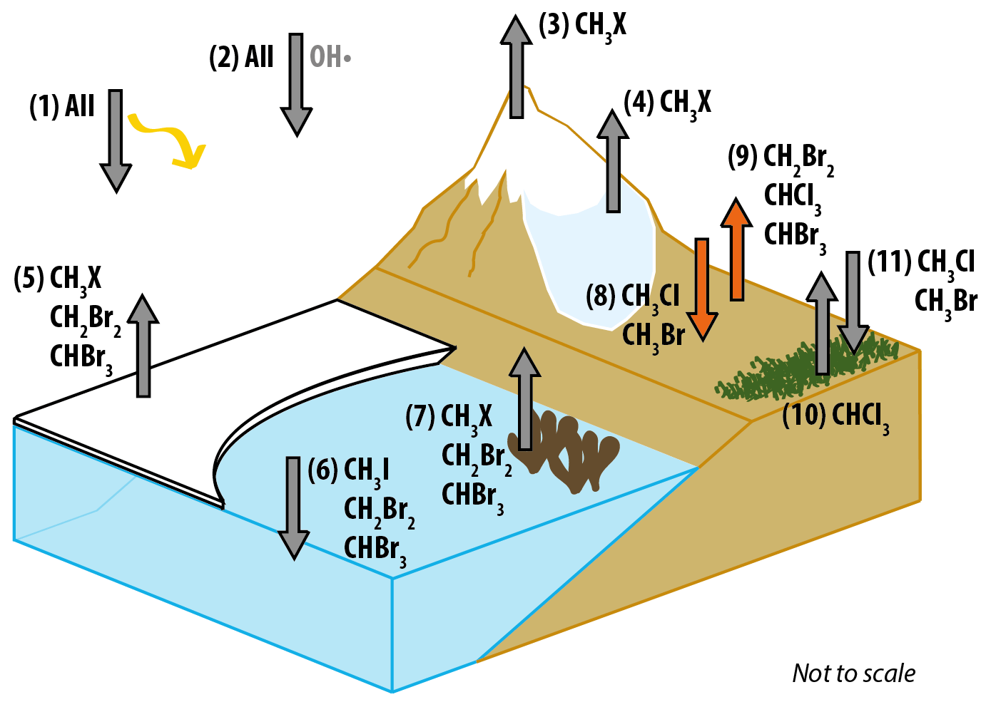
Figure 7 Schematic diagram summarising natural sources and sinks for the six halocarbons of interest in polar regions with fluxes measured in this paper (8 and 9) highlighted in orange. The sources and sinks are as follows: (1) UV photolysis sink, (2) reaction with OH• sink, (3) photochemistry in snow source, (4) microbial activity in snow source, (5) sea ice microalgae source, (6) open-ocean sink, (7) macroalgae source, (8) forefield sink, (9) forefield source, (10) tundra source, (11) tundra sink. (CH₃X = CH₃Cl, CH₃Br, CH₃I). References for the presence of each flux are as follows: 1, 2 (see Montzka et al., 2011, for review), 3 (Swanson et al., 2007), 4 (Redeker et al., 2017), 5 (Laturnus et al., 1998; Sturges et al., 1993), 6 (Stemmler et al., 2014; Ziska et al., 2013), 7 (Laturnus, 1996, 2001), 8 and 9 (this study), 10 (Albers et al., 2017; Rhew et al., 2008), 11 (Rhew et al., 2007).

This pattern where sites with younger, less-developed soils have similar fluxes to the older and developed soil of the tundra site also occurred for CHCl₃ and CHBr₃ where the highest mean fluxes were measured at the established mat site and the disturbed mat site, respectively, but were statistically similar to the flux measured at the tundra site (p=0.1, 0.6, respectively). This is even more surprising for the disturbed mat site which is completely bare of vegetation and has comparatively low bacterial cell numbers (Fig. 4g). Terrestrial fluxes of CHBr₃ have rarely been measured (see Sect. 5.2), whereas CHCl₃ emissions have been recorded, including from the Alaskan tundra where the average flux was 45 nmol m⁻² d⁻¹ (Rhew et al., 2008). Mean emissions of CHCl₃ were larger at the tundra and established mat sites and similar at the disturbed mat site (74, 106, and 43 nmol m⁻² d⁻¹, respectively). Considerable variability of CHCl₃ fluxes was measured, with the range for the tundra site being 23 to 128 nmol m⁻² d⁻¹ and the range for established mat site being 64 to 183 nmol m⁻² d⁻¹. This variability in CHCl₃ fluxes is less than, but comparable to, the variation measured at the Alaskan tundra of <1 to 260 nmol m⁻² d⁻¹ (Rhew et al., 2008). We have demonstrated that younger surfaces can be sources of CHCl₃ and CHBr₃ and sinks of CH₃Cl and CH₃Br despite their lesser soil development and lower microbial and plant presence. In particular, it appears the presence of cyanobacterial mats negates the requirement for a more developed soil. To our knowledge, no studies have been conducted upon halogenated trace gas fluxes from cyanobacteria mats or freshwater cyanobacteria, although marine cyanobacteria have been suggested to be involved in production of CH₂Br₂, CHBr₃, and CH₃I (Karlsson et al., 2008; Roy et al., 2011). Determining if cyanobacteria themselves, or other microorganisms present in the mat, are responsible for the elevated fluxes was beyond the scope of this study.

5.2 Terrestrial emission of typically marine-origin brominated compounds

A second novel finding of this study was the emission of CHBr₃ and CH₂Br₂ across the glacier forefield, with very small emissions at the snout site but more appreciable fluxes at all other sites (Fig. 5e–f). CHBr₃ and CH₂Br₂ are typically attributed to marine sources (Law et al., 2006). However, there have been limited observations of emission of both compounds from terrestrial environments. CHBr₃ has been observed to be emitted from rice paddies, with algae in the water column as the suggested source; however a rice-mediated production mechanism was not discounted (Redeker et al., 2003). CH₂Br₂ emissions have been observed from wet temperate peatlands, with no production mechanism suggested (Dimmer et al., 2001). Emission of CHBr₃ has been observed, but not quantified, from the transitional terrestrial–marine environment of a coastal wetland, where it was shown to be abiogenic in origin (Wang et al., 2016). Further, abiogenic production of CHBr₃ through the oxidation of organic matter by Fe(III) and H₂O₂ when halide ions are present has been documented in a laboratory-based soil study (Huber et al., 2009). The largest flux of CH₂Br₂ is measured at the tundra site which is analogous to an Arctic peatland ecosystem and thus complements the emissions measured from temperate peatlands in Ireland (Dimmer et al., 2001). Our results provide further evidence of the emission of these two compounds in a terrestrial environment and the first evidence of terrestrial emission of these compounds in the Arctic.

5.3 Controls on halocarbon fluxes across the forefield

5.3.1 Biological consumption of methyl halides and abiogenic production of CH₃I

Methyl halides were primarily consumed on the glacier forefield, with all three compounds consistently consumed at the established mat and tundra sites but with fluxes of CH₃I in both directions at the snout, pond mat, and disturbed mat sites. The strong inter-correlations between different methyl halides suggest a similar consumption mechanism, particularly between CH₃Cl and CH₃Br. Strong correlations between CH₃Cl and CH₃Br have been found elsewhere, including in the Alaskan tundra, with similar suggestions of common consumption mechanisms or common limiting factors (Rhew et al., 2007). We suggest that the consumption of all three methyl halides observed across the forefield is driven by prokaryotic degradation, which is supported by methyl halide fluxes being correlated with bacterial cell concentrations ($r<-\mathrm{0.52}$) and net microbial respiration (CO₂ emission; $r<-\mathrm{0.41}$, not significant for CH₃I). Both biogenic and abiogenic (through organic matter oxidation) soil production mechanisms of CH₃I have previously been demonstrated (Amachi et al., 2001; Keppler et al., 2000). However, these mechanisms are not strongly supported here as CH₃I is emitted at the sites (snout, pond mat, disturbed mat) with the lowest bacterial concentrations and lowest organic matter contents (0.1 %–0.6 %). Identifying the CH₃I production mechanism would require further study.

5.3.2 Inconclusive influence of water content on methyl halide fluxes

Several studies have identified the importance of soil water content for CH₃X fluxes, with very low water contents limiting biological activity and high water contents limiting the mass transfer of reactants during CH₃X formation and degradation (Khan et al., 2012; Rhew et al., 2010; Teh et al., 2009). We find that increasing water content was correlated to greater consumption of CH₃X across all sites, despite high water contents (>40 % v∕v). This is driven largely by high water contents at the tundra site where the highest consumption of CH₃X was found, presumably due to the more developed soils and biota at this site. Within the tundra site the relationship with water content persists, in contrast to the Alaskan tundra studies which found that decreasing water content was the key factor causing increased consumption of CH₃Cl and CH₃Br (Teh et al., 2009). Our results are not consistent with this finding, perhaps due to the noise caused by a small within-site sample size (n=8) coupled with a smaller range of water volumes measured here (40 %–60 %, compared to <30 to >70 % in the Alaskan study). Further, the relationship between CH₃X and water content implied greater consumption in more anoxic soils; however, higher consumption of CH₃X was found to occur where fluxes of CH₄ are tending towards the aerobic process of consumption, as found in the Alaskan tundra (Rhew et al., 2007). The contradiction between water content and aerobic CH₄ consumption shown here further indicates that more within-site data are required, as the disparity in the CH₃X fluxes of the different sites drives the all-site relationships.

5.3.3 Biogenic and abiogenic production of poly-halogenated species

Biogenic production mechanisms of CHCl₃, CHBr₃, and CH₂Br₂ are shared (haloperoxidase activity), as is the abiogenic production mechanism of the haloforms (CHX₃; Huber et al., 2009; Manley, 2002). If either biogenic or abiogenic processes were the sole source of the poly-halogenated species, then we would expect that, at least, CHX₃ fluxes would be correlated. However, CHCl₃ and CHBr₃ are not well-correlated across all sites (r=0.29, p>0.05), suggesting different sources of these compounds within or between sites. Here, CHCl₃ is strongly correlated to bacterial cell numbers, but CHBr₃ is not, which tentatively suggests that CHCl₃ is produced biologically. At the established mat and tundra sites, CHCl₃ and CHBr₃ were not significantly correlated, suggesting multiple sources or a possible unknown consumption process. There is no evidence prior to this study that terrestrial or freshwater cyanobacteria are involved in halocarbon production. However, marine cyanobacteria have been implicated in the production of CHBr₃ and CH₂Br₂, and the bromoperoxidase enzyme has been identified in some marine species (Johnson et al., 2011; Karlsson et al., 2008). The highest emissions of CH₂Br₂ at the tundra site could be due to a different microbial community make-up or a plant-mediated process. We suggest that a possible mixture of abiogenic and biogenic production mechanisms are responsible for CHCl₃ and CHBr₃ emissions, whereas CH₂Br₂ emissions seem more likely to be driven biologically.

5.4 Glacier forefields as a source and sink of halocarbons?

Determining the local or regional importance of forefield halocarbon fluxes would require further study into diurnal, seasonal, and spatial variations. However, estimations of the yearly regional source or sink of each gas is still worthwhile, particularly for CHBr₃ and CH₂Br₂ for which no prior fluxes have been measured from terrestrial Arctic environments. We calculate an Arctic tundra source of 0.11 and 0.09 Gg Br yr⁻¹ for CHBr₃ and CH₂Br₂, assuming that no production occurs outside of the growing season (Sect. 3.6.2). The sources are minor compared to the estimated global sources of 120–820 Gg Br yr⁻¹ for CHBr₃ and 57–100 Gg Br yr⁻¹ for CH₂Br₂, which are primarily oceanic in origin (Carpenter et al., 2014; Engel et al., 2018). To determine if our tundra source has regional significance, we estimate the proportion of the global flux that may occur in the Arctic assuming the global source is equally distributed over the Earth's surface and using an Arctic surface area (area north of the Arctic circle) of 4 % of the Earth's total. The tundra source would be an estimated 0.3 %–2 % of CHBr₃ and 2 %–4 % of CH₂Br₂ of the estimated total Arctic source of 5–33 Gg Br yr⁻¹ for CHBr₃ and 2–4 Gg Br yr⁻¹ for CH₂Br₂. Further, global sources are dominantly marine, and although Arctic macroalgae are a source of both gases (Laturnus, 1996), polar oceans as a whole have been suggested to be a sink (e.g. Chuck et al., 2005; Ziska et al., 2013; Fig. 7). Therefore, a terrestrial Arctic source could be more regionally important than estimated here.

For the other halocarbons analysed across the glacier forefield, we calculated a potential regional forefield flux from an estimated Arctic forefield land area (Sect. 3.6.1). Small net sinks of 8 t yr⁻¹ of CH₃Cl, 0.2 t yr⁻¹ of CH₃Br, and 0.01 t yr⁻¹ of CH₃I and small net sources of 18 t yr⁻¹ of CHCl₃, 0.2 t yr⁻¹ of CH₂Br₂, and 0.3 t yr⁻¹ of CHBr₃ were calculated. All of these are minor compared to global fluxes, due to the relatively small area of land covered by glacier forefields. Fluxes from the Alaskan tundra, which were similar to our fluxes for established mat and tundra, were found to be regionally important, where they represent the equivalent of approximately 20 %–25 % and 10 %–15 % of the seasonal variation in the Arctic troposphere of CH₃Cl and CH₃Br, respectively (Rhew et al., 2007). However, our estimated forefield land surface area is 2 orders of magnitude smaller than the estimated area of Arctic tundra (7.3×10¹² m²), meaning even within the Arctic troposphere the glacier forefield sink of CH₃Cl and CH₃Br is insignificant.

Although our daily fluxes are likely an underestimate (due to calculation from concentration change over 1 h, after the rate of change had slowed; Sect. 3.3), the magnitude of this underestimate will not be large enough to alter the significance of the total gas fluxes regionally. Despite all halocarbons studied here appearing to represent only minor fluxes globally and regionally, this study has shown the potential for younger surfaces to be involved in halocarbon flux processes, which may become more important due to expansion of these surfaces under future warming.

6 Conclusions

We present the first measurements of halocarbon fluxes from glacier forefield land surfaces, showing an overall net sink of CH₃Cl, CH₃Br, and CH₃I and net source of CHCl₃, CHBr₃, and CH₂Br₂. Relatively young, underdeveloped soils exposed by glacial retreat can have similar fluxes of halocarbons to older, more developed soils, particularly where cyanobacterial mats have formed. We have shown that surfaces covered in these mats are sinks of CH₃Cl, CH₃Br, and CH₃I and sources of CHCl₃ and CHBr₃. The latter two gases also show appreciable fluxes even from bare sediment adjacent to cyanobacterial mats. This is the first research known to us conducted on terrestrial cyanobacteria, and additionally we have provided rare terrestrial flux measurements of CHBr₃ and CH₂Br₂. Future work should identify whether cyanobacteria themselves or other microbes are responsible for the high fluxes over the mats; improve the spatial and temporal distribution of these measurements, including conducting measurements outside the growing season; conduct gas analyses at less than 1 h intervals to reduce the suspected underestimation of the flux calculations; and whether other terrestrial environments emit CHBr₃ and CH₂Br₂, particularly in areas where the fluxes might be higher (i.e. in more developed and more active soils) and therefore more regionally important. The significance of glacier forefield fluxes may become more important in the future with continuing change in the Arctic and the resultant retreat of glacial systems and exposure of land.