the Creative Commons Attribution 4.0 License.
the Creative Commons Attribution 4.0 License.
 | 27 Feb 2020
Evaluation of NU-WRF model performance on air quality simulation under various model resolutions – an investigation within the framework of MICS-Asia Phase III
Mian Chin
Tom Kucsera
Dongchul Kim
Huisheng Bian
Jun-ichi Kurokawa
Yuesi Wang
Zirui Liu
Gregory R. Carmichael
Zifa Wang
Hajime Akimoto
Horizontal grid resolution has a profound effect on model performances on meteorology and air quality simulations. In contribution to MICS-Asia Phase III, one of whose goals was to identify and reduce model uncertainty in air quality prediction, this study examined the impact of grid resolution on meteorology and air quality simulation over East Asia, focusing on the North China Plain (NCP) region. The NASA Unified Weather Research and Forecasting (NU-WRF) model has been applied with the horizontal resolutions at 45, 15, and 5 km. The results revealed that, in comparison with ground observations, no single resolution can yield the best model performance for all variables across all stations. From a regional average perspective (i.e., across all monitoring sites), air temperature modeling was not sensitive to the grid resolution but wind and precipitation simulation showed the opposite. NU-WRF with the 5 km grid simulated the wind speed best, while the 45 km grid yielded the most realistic precipitation as compared to the site observations. For air quality simulations, finer resolution generally led to better comparisons with observations for O3, CO, NOx, and PM2.5. However, the improvement of model performance on air quality was not linear with the resolution increase. The accuracy of modeled surface O3 of the 15 km grid was greatly improved over the one from the 45 km grid. A further increase in grid resolution to 5 km, however, showed diminished impact on model performance improvement on O3 prediction. In addition, a 5 km resolution grid showed large advantage in better capturing the frequency of high-pollution occurrences. This was important for the assessment of noncompliance with ambient air quality standards, which was key to air quality planning and management. Balancing the modeling accuracy and resource limitation, a 15 km grid resolution was suggested for future MICS-Asia air quality modeling activity if the research region remained unchanged. This investigation also found a large overestimate of ground-level O3 and an underestimate of surface NOx and CO, likely due to missing emissions of NOx and CO.
- Article
(5929 KB) - Full-text XML
-
Supplement
(957 KB) - BibTeX
- EndNote


Air pollution is a threat to human health and climate and detrimental to ecosystems (Anenberg et al., 2010; https://www.who.int/airpollution/ambient/en/, last access: 24 February 2020). Lelieveld et al. (2015) estimated that over 3 million premature deaths could be attributable to outdoor air pollution worldwide in 2010 based on their analysis of data and the results from a high-resolution global air quality model. Since the turn of the 21st century, East Asia has undergone remarkable changes in air quality as observed by satellite and ground stations (Jin et al., 2016; Krotkov et al., 2016). In the past decade, haze (fine particle) pollution has become a household name in China and many severe haze events have been reported and their formation mechanisms and associations with global- and meso-scale meteorology have been analyzed (Zhao et al., 2013; Huang et al., 2014; Gao et al., 2016; Cai et al., 2017; Zou et al., 2017). Meanwhile, ground-level ozone has been a major air quality concern in China (Wang et al., 2017; Lu et al., 2018), Japan (Akimoto et al., 2015), and South Korea (Seo et al., 2014). In combination with observations from various platforms, chemical transport models (CTMs) remain an important tool to understand mechanisms, to investigate spatial–temporal distributions, and to design feasible control strategies of air pollution. However, CTM uncertainties persist (e.g., Carmichael et al., 2008) and the interpretation of any model results needs caution and the exertion of careful analysis.
Intermodel comparison study provides a valuable way to understand model uncertainties and sheds light on model improvements. With these as two of its major goals, the Model Inter-Comparison Study for Asia (MICS-Asia) was initiated in 1998. Since then MICS-Asia has gone through three phases with emphasis on various aspects of air pollution. Phase I focused on long-range transport and deposition of sulfur over East Asia (Carmichael et al., 2002). Phase II expanded the analysis to more pollutants, including nitrogen compounds, particulate matter, and ozone, in addition to sulfur (Carmichael et al., 2008). Moving fast to Phase III, MICS-Asia concentrated on three topics with the first aiming at identifying strengths and weaknesses of current air quality models to provide insights into reducing uncertainties (Gao et al., 2018). There were a total of 14 CTMs – 13 regional and 1 global – participating in the coordinated model experiment, which simulated air quality over Asia throughout the year 2010. Due to the constraints of computing resources among participating modeling groups, a 45 km horizontal resolution has been adopted by every team to run the year-long experiment.
This relatively coarse spatial resolution raises the question of how representatively the model can resolve key issues relevant to air quality and its planning and regulation, e.g., heterogeneous emissions, inhomogeneous land cover, and meteorology. For example, Valari and Menut (2008) explored the question using the CHIMERE chemistry transport model at various horizontal resolutions over Paris. They found that the ozone simulation was especially sensitive to the resolution of emissions. However, the benefit of increasing emission resolutions to improve ozone forecast skills was not monotonic and at a certain point the forecast accuracy decreased upon further resolution increase. Using the Weather Research and Forecasting–Chemistry (WRF–Chem) model with various horizontal resolutions (3–24 km) over Mexico City, Tie et al. (2010) concluded that a 1 to 6 ratio of grid resolution to city size appeared to be a threshold to improve ozone forecasting skill over megacity areas: the forecast would be improved significantly when model resolution was below this threshold value. Contrary to Valari and Menut (2008), Tie et al. (2010) suggested that the meteorology changes associated with the grid size choice played a more prominent role in contributing to the improvement of ozone forecast skills. More recently, Neal et al. (2017) employed a high-resolution (12 km) air quality model with high-resolution emissions within the Met Office's Unified Model for air quality forecasting (AQUM) over Great Britain. They found that AQUM improved significantly the forecast accuracy of primary pollutants (e.g., NO2 and SO2) but less obviously the forecast accuracy of secondary pollutants like ozone, as compared with a regional composition–climate model (RCCM, 50 km horizontal resolution). But there was a drawback to their conclusion in that the chemical mechanisms and photolysis rates utilized in AQUM and RCCM were different, complicating the underlying reasons for changes in forecast skills. Lee et al. (2018) examined the importance of aerosol–cloud–radiation interactions to precipitation and the model resolution impact of key meteorological processes that affected precipitation using the Advanced Research WRF model. They found that the coarse model resolution would lower updraft, alter cloud properties (e.g., mass, condensation, evaporation, and deposition), and reduce cloud sensitivity to ambient aerosol changes. They further concluded that the uncertainty associated with resolution was much more than that related to cloud microphysics parameterization. The resultant meteorological condition change would trigger an air quality response as well.
Despite the progress, the exploration of impacts of model resolution on local air quality over Asia is rare. Taking advantage of the MICS-Asia platform, we examined the issue over the MICS-Asia domain using the NASA Unified WRF (NU-WRF) model (Tao et al., 2013, 2016, 2018; Peters-Lidard et al., 2015), focusing on the North China Plain (NCP) which was plagued by frequent heavy air pollution episodes. The investigation would not only assist in gaining insights into how model horizontal resolution affects simulated meteorology and air quality but also contribute to the formulation of uncertainties resulting from model resolutions for the MICS-Asia community. The latter would especially be valuable since most MICS-Asia Phase III model simulations were conducted at a specific horizontal resolution (i.e., 45 km for most participants).
NU-WRF is an integrated regional Earth-system modeling system developed from the advanced research version of WRF–Chem (Grell et al., 2005), which represents atmospheric chemistry, aerosol, cloud, precipitation, and land processes at convection-permitting spatial scales (typically 1–6 km). NU-WRF couples the community WRF–Chem with NASA's Land Information System (LIS), a software framework including a suite of land surface models (LSMs) that are driven by satellite and ground observations and reanalysis data (Kumar et al., 2006; Peters-Lidard et al., 2007). It also couples the Goddard Chemistry Aerosol Radiation and Transport (GOCART) bulk aerosol scheme (Chin et al., 2002, 2007) with the Goddard radiation (Chou and Suares, 1999) and microphysics schemes (Tao et al., 2011; Shi et al., 2014), which allows for fully coupled aerosol–cloud–radiation interaction simulations. In addition, NU-WRF links to the Goddard Satellite Data Simulator Unit (G-SDSU), which converts simulated atmospheric profiles, e.g, clouds, precipitation, and aerosols, into radiance or backscatter signals that can be directly compared with satellite level-1 measurements at a relevant spatial and temporal scale (Matsui et al., 2009, 2013, 2014). In this study, NU-WRF has been employed to carry out the model simulations at various horizontal resolutions using the same set of physical and chemical configurations.
A nested domain setup was configured for this investigation as shown Fig. 1. The 45 km resolution mother domain (d01) covered the MICS-Asia Phase III study region. The nested 15 km (d02) and 5 km (d03) domains covered East Asia and the NCP, respectively. A one-way nesting approach was applied so that the values of the mother domains were independent of those of the respective nested domains. This analysis focused on the NCP and its adjacent areas, with a total area of over 1.1 million square kilometers. The key NU-WRF configurations included the updated Goddard cumulus ensemble microphysics scheme (Tao et al., 2011), the new Goddard long- and shortwave radiation schemes (Chou and Suares, 1999), the Monin–Obukhov surface layer scheme, the unified Noah land surface model (Ek et al., 2003) with LIS initialization (Peters-Lidard et al., 2015), the Yonsei University planetary boundary layer scheme (YSU; Hong et al., 2006), the new Grell cumulus scheme developed from the ensemble cumulus scheme (Grell and Devenyi, 2002) that allowed subsidence spreading (Lin et al., 2010), the second-generation regional acid deposition model (RADM2; Stockwell et al., 1990; Gross and Stockwell, 2003) for trace gases, and GOCART for aerosols. In this investigation, the option of fully coupled GOCART–Goddard microphysics and radiation schemes (Shi et al., 2014) was implemented to account for the aerosol–cloud–radiation interactions.
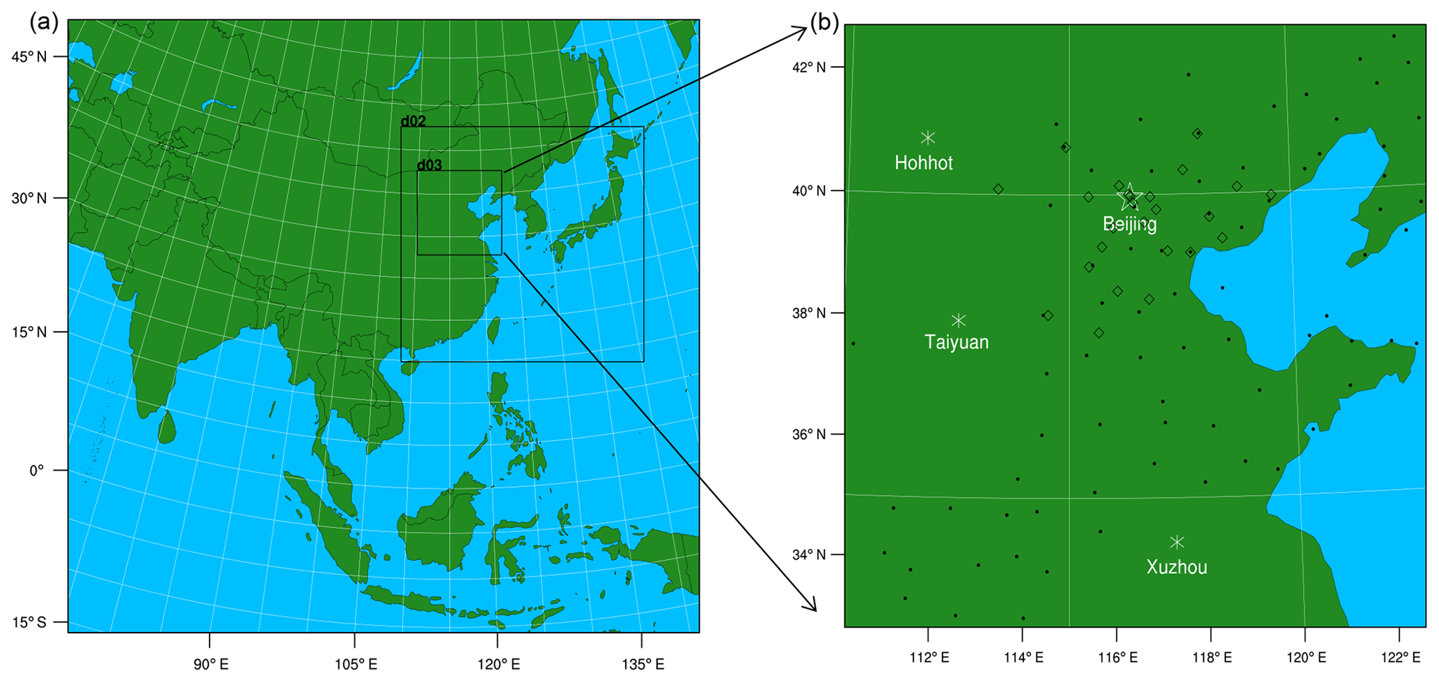
Figure 1NU-WRF domain setup. (a) The nested MICS-Asia domains, (b) the enlarged NCP domain (d03) with diamonds representing the air quality monitoring sites and black dots denoting the meteorological stations. Locations of four cities are marked for position reference.
Anthropogenic emissions were from the mosaic Asian anthropogenic emission inventory (MIX; Li et al., 2017) that was developed for MICS-Asia Phase III. The MIX inventory was at the 0.25∘ by 0.25∘ resolution and was projected to the study domain under the 45, 15, and 5 km horizonal resolutions. Fire emissions were from the 0.5∘ by 0.5∘ Global Fire Emissions Database version 3 (GFEDv3; van der Werf et al., 2010; Mu et al., 2011) and were also projected to the targeted region. Biogenic emissions were computed online using the Model of Emissions of Gases and Aerosols from Nature version 2 (MEGAN2; Guenther et al., 2006). Dust and sea salt emissions were also calculated online using the dynamic GOCART dust emissions scheme (Kim et al., 2017) and sea salt scheme (Gong, 2003), respectively.
The meteorological lateral boundary conditions (LBCs) were derived from the Modern-Era Retrospective analysis for Research and Applications (MERRA; Rienecker et al., 2011). The trace gas LBCs were based on the 6 h results from the Model for OZone And Related chemical Tracers (MOZART; Emmons et al., 2010). The aerosol LBCs were from the global GOCART simulation with a resolution of 1.25∘ (longitude) by 1∘ (latitude; Chin et al., 2007) updated every 6 h. Three horizontal resolutions varied from 45 to 5 km with 15 km in between. Sixty terrain-following vertical levels stretched from the surface to 20 hPa with the first-layer height at approximately 40 m from the surface. The simulation started on 20 December 2009 and ended on 31 December 2010, with the first 11 d as the spin-up.
3.1 Comparisons with observations
The NU-WRF results of different horizontal resolutions have been compared with ground observations using the following statistical measures.
Here, mi and oi denote the modeled and observed values at time–space pair i; and represent the average modeled and observed values, respectively. The term r describes the strength and direction of a linear relationship between two variables; a perfect correlation has a value of 1. NMB and MB depict the mean deviation of modeled results from the respective observations. A perfect model simulation yields a NMB and a MB of 0. RMSE measures the absolute accuracy of a model prediction. The smaller the RMSE, the better the model performance is. Similar to NMB and MB, a RMSE of 0 indicates a perfect model prediction. NSD is a measure to check how well the model can reproduce the variations of observations; a value of 1 represents a perfect reproduction of observed variations.
3.1.1 Meteorology
The 2010 meteorological observations were collected at the standard stations operated by the China Meteorological Administration (CMA; http://data.cma.cn/en, last access: 24 February 2020). The locations of each site within our study domain were represented by the black dots in Fig. 1b. In total there were 77 sites reporting daily average values of wind speed (Wind), air temperature (Temp), and relative humidity (RH), as well as daily total precipitation (Precip). Figure 2a shows the Taylor diagram summarizing r, NMB, and NSD of the comparison of regional mean (average of observations from 77 sites) daily meteorological variables. Along the azimuthal angle is r. NSD is proportional to the radial distance from the origin. NMB (sign and range) is represented by the geometric shapes. The statistical measures under 45, 15, and 5 km resolutions are represented by the colors blue, green, and red, respectively. The closer to the point Obs on the Taylor diagram and the smaller the NMB, the better the model performance is.
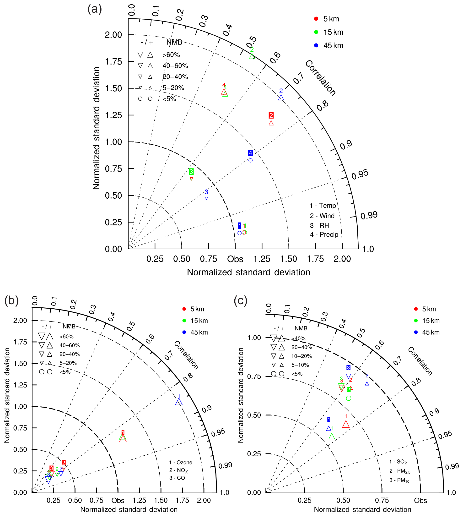
Figure 2Taylor diagrams for evaluations of NU-WRF performances on meteorology (a) and air quality (b, c) simulations at three resolutions for the year of 2010.
It can be seen that the model horizontal resolution has little impact on surface air temperature simulation. Regardless of resolution selections, the modeled temperature correlated very well with the corresponding observations with r values all approaching 0.99. NU-WRF also reproduced the observed temperature variations well with NSD ranging between 1.05 and 1.10. Meanwhile, NMB was within ±1 % for all experimented resolutions. RMSEs were 1.13, 2.26, and 2.02 K for the 45, 15, and 5 km grids, respectively. The insensitivity of surface air temperature to the choice of model resolutions was also reported by Gao et al. (2017), who used WRF to explore the issue for summer seasons at the 36, 12, and 4 km resolutions.
On the other hand, the horizontal resolution has a remarkable effect on surface wind speed as shown in Fig. 2a. At the 5 km resolution, NU-WRF yielded an r value of 0.75, NMB of approximately 54 %, and NSD of 1.78. NU-WRF simulated a larger variation in wind than the observations showed. As comparisons, the values of r, NMB, and NSD for 15 and 45 km were 0.54, 95 %, and 2.14 and 0.71, 103 %, and 2.01, respectively. The respective RMSEs of the 45, 15, and 5 km grids were 2.87, 2.82, and 1.67 m s−1. It was apparent that the 5 km resolution gave the overall best wind speed simulation compared to the observations, though NU-WRF overestimated the surface wind speed in all cases. The wind speed overestimate, especially under low wind conditions, was a common problem in all MICS-Asia participating models and other weather forecast models (Gao et al., 2018). This overestimate stemmed from many factors, including but not limited to terrain data uncertainty, poor representation of urban surface effect, and horizontal and vertical grid resolutions. Yu (2014) in her doctoral dissertation pointed out that surface wind simulation would be improved upon using more accurate land-use data. This is expected since surface wind is largely dependent on the land surface characteristics, such as albedo and roughness. High-resolution grids tend to have more accurate land-use representation because they recognize the inhomogeneous nature of land type.
NU-WRF simulations at all three resolutions yielded similar reproductions of the observed variations in relative humidity (RH) with NSD ranging between 0.87 and 0.88. The modeled RH was less variable than the observed one. While the modeled RH at the 45 km resolution (r=0.84) better correlated with the observations than those at the finer resolutions did (approximately 0.67 for both 15 and 5 km resolutions), the NMB at this resolution was the largest (−17 %) among the three cases. The NMBs for the 15 and 5 km cases were −10 % and −12 %, respectively. Overall, NU-WRF underestimated the surface RH. The respective RMSEs for 45, 15, and 5 km resolutions were 13.2 %, 12.6 %, and 13.3 %. The simulation with the 15 km grid appeared to yield the overall best RH in all three cases.
It was interesting to find that NU-WRF simulated the precipitation best, as directly compared to the rain gauge data, when using the 45 km grid. At this resolution, NU-WRF gave r of 0.81, NMB of 1.7 %, RMSE of 3.2 mm d−1, and NSD of 1.41. As comparisons, the values of r, NMB, RMSE, and NSD for 15 and 5 km were 0.53, 76 %, 5.7 mm d−1, and 1.71 and 0.52, 80 %, 5.8 mm d−1, and 1.72, respectively. Finer resolutions indeed yielded worse results in precipitation modeling as compared to the site data. This may be because precipitation was a very heterogeneous phenomenon: finer model grids had larger chances of missing a precipitation event or hitting an event that was nonexistent, leading to a greater overall bias and a poorer correlation. On the contrary, Gao et al. (2017) compared their WRF modeled results to the gridded precipitation based on the daily rain gauge data that were gridded to the 0.125∘ resolution using the synergraphic mapping algorithm with topographic adjustment to the monthly precipitation climatology (Maurer et al., 2002). They reported that the modeled precipitation of the 4 km resolution was much improved over that of the coarser 36 or 12 km resolutions.
The time series of daily mean wind speed, air temperature, and RH, as well as daily total precipitation averaged over the monitoring sites are illustrated in Fig. S1 in the Supplement. They echoed the above findings based on the Taylor diagram. It appeared that NU-WRF constantly overestimated surface wind speed throughout the year with large overestimates occurring in fall and winter, while it severely underestimated RH in summer. Uncertainty in representation of land surface characteristics at least partially explained these biases (Yu, 2014; Gao et al., 2018). High-resolution grids tended to reduce the uncertainty in land surface representation, which would be helpful for improving model performance in meteorology simulation. A more detailed exploration of model–observation mismatch would be insightful but was beyond the scope of this research.
3.1.2 Air quality
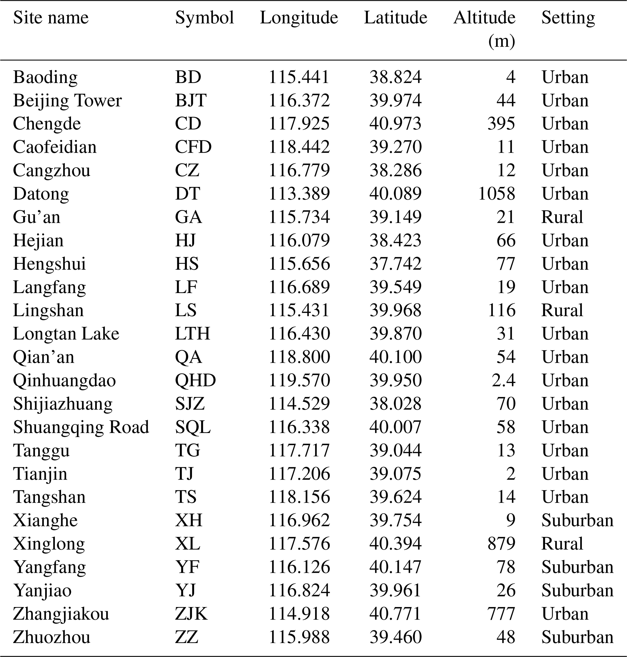
The difference seen in the aforementioned meteorology would cause varied performances of air quality simulations at various model horizontal resolutions. In this study, the NU-WRF simulated surface air quality was compared to the corresponding observations. The 2010 ground-level air quality data were obtained from the Chinese Ecosystem Research Network (CERN; http://www.cern.ac.cn, last access: 25 February 2020) operated by the Institute of Atmospheric Physics of the Chinese Academy of Sciences. There were 25 monitoring sites distributed within a 500 km by 500 km area centering around Beijing, China (open diamonds in Fig. 1b). The site locations and characteristics were listed in Table 1. Of the 25 sites, 22 were either in an urban or a suburban setting with the rest being in a rural setting. Each site reported hourly concentrations of at least one of the following six pollutants: ozone (O3), nitrogen oxides (NOx), carbon monoxide (CO), sulfur dioxide (SO2), and particulate matters with aerodynamic diameters less than 2.5 and 10 µm (PM2.5 and PM10).
(a) Regional average
First, the regional mean (averaged across 25 sites) daily surface concentrations from both observations and simulations, paired in space and time, were calculated. The r, NMB, and NSD were then computed and illustrated in a Taylor diagram (Fig. 2b, c).
The six pollutants can be put into two groups: one most relevant to ozone photochemistry including O3, NOx, and CO and the other closely tied to aerosols including SO2, PM2.5, and PM10. It was readily seen that the r values of O3, NOx, and CO were not very sensitive to the choice of model horizontal resolutions. For O3, the r values for 45, 15, and 5 km grids were all around 0.85. The respective r values were 0.84, 0.81, and 0.80 for NOx and 0.80, 0.75, and 0.73 for CO. In general, however, NU-WRF reproduced the observed variations in O3, NOx, and CO better with a fine resolution than with a coarse one. An NSD of 1.23 for O3 at the 5 km resolution was the closest to 1 among the three resolutions (1.24 for 15 km and 2.01 for 45 km). NSDs were 0.40, 0.36, and 0.46 for NOx and 0.24, 0.27, and 0.31 for CO, under the 45, 15, and 5 km resolutions, respectively, suggesting that simulations with the finest resolution tended to reproduce the observed variations better than the ones with coarse resolutions for these three trace gases. Meanwhile, NU-WRF yielded the smallest bias when employing the fine-resolution grid. NMBs for O3 decreased from 115 % to 92 % when grid resolutions increased from 45 to 5 km. NMBs were −38 %, −30 %, and −18 % for NOx and −61 %, −55 %, and −51 % for CO, under the 45, 15, and 5 km resolutions, respectively. It was apparent that NU-WRF overestimated surface O3 but underestimated NOx and CO, consistent with the findings in the companion MICS-Asia Phase III studies that based their results on ensemble model simulations (Li et al., 2019; Kong et al., 2020). The majority of the air quality monitoring sites used in this study were in an urban setting, which typically were in a VOC-limited regime. This meant that the underestimate of NOx would reduce the titration that consumed surface O3, leading to its overestimate. We further analyzed the model bias for daytime (08:00–18:00 LT) vs. nighttime. It was found that the nighttime biases for surface O3 and NOx were approximately 2–4 times higher than those of the daytime, consistent with the finding that insufficient NOx titration caused an overestimate of modeled surface O3.
NU-WRF simulated fewer variations in the three aerosol-related pollutants than those of observations under all applied horizontal resolutions. The NSDs ranged from 0.56 (for SO2 at 15 km resolution) to 0.96 (for PM2.5 at 45 km resolution). Though it reproduced the observed SO2 variations the best (NSD = 0.68) with the 5 km resolution, NU-WRF yielded the best NSD for PM2.5 (0.96) and PM10 (0.92) when the 45 km resolution was employed. Similar to three trace gases relevant to surface O3 formation, the choice of model resolution had a limited effect on r statistics. The r values varied from 0.70 (45 km resolution) to 0.76 (both 15 and 5 km resolution) for surface SO2 and from 0.68 (45 km resolution) to 0.63 (5 km resolution) for PM2.5. The r values for PM10 were all around 0.58 under the selected resolutions. The impact of model resolution on NMBs showed mixed information: while the smallest NMBs for SO2 (20 %) and PM10 (−19 %) were achieved using the 45 km resolution, the smallest NMB for PM2.5 (1.5 %) was observed at the 15 km resolution. The model underestimate of PM10 was consistent with the findings of the companion investigation using the multimodel ensemble analysis (Chen et al., 2019).
Figure S2 shows the time series of daily mean air quality averaged over the monitoring sites for the year 2010. The constant underestimate of CO throughout the year, severe underestimate of NOx in fall and winter, and large underestimate of SO2 in summer all indicated that the emissions inventory may be incomplete, agreeing with the reports by Kong et al. (2020) and Li et al. (2019). In the future, improvement of the emissions inventory accuracy and a more realistic temporal emissions distribution may help improve NU-WRF performance in simulating O3 photochemistry.
(b) Individual sites
The daily average concentrations of each pollutant were calculated and paired in space and time at each air quality monitoring site. Then the statistics at each individual site were computed.
Figure 3 illustrates the comparisons of MB, RMSE, and correlation coefficient r of surface O3 from different horizontal resolutions at each site. It can be found that there was no single resolution that yielded the best correlation across all sites. For example, the simulation with the 45 km horizontal resolution gave the best correlation over sites BD, CFD, CZ, HJ, SJZ, SQL, TG, TJ, TS, XH, XL, YF, YJ, and ZJK. At the other end of spectrum, BJT, DT, and LTH achieved the best correlation when the 5 km grid was applied. QHD saw the best correlation of the simulation with the 15 km resolution. In any case, however, the variations in r values from different horizontal resolutions at each site were small (less than 0.04). On the other hand, NU-WRF yielded the worst MB and RMSE when employing the 45 km resolution grid, while MB and RMSE were similar across simulations with 15 and 5 km resolutions. Typically, at sites with urban or suburban settings, MB (RMSE) based on the 45 km grid was approximately 15 %–30 % (20 %–40 %) higher than that of the 15 or 5 km grids. It appeared that NU-WRF tended to have a better performance of ground-level O3 simulation when increasing the horizontal resolution from 45 to 15 km, but further finer resolution had diminished impact on improving surface O3 modeling. This was consistent with the finding by Valari and Menut (2008), who concluded that the benefit of finer-horizontal-resolution grids for improving surface O3 forecast skill would diminish at a certain point.

Figure 3Comparisons of MB, RMSE, and correlation coefficient r of surface O3 from different horizontal resolutions at each air quality monitoring site for the year of 2010.
Figure 4 shows the PM2.5 case of comparisons of MB, RMSE, and r. Only 10 sites reported PM2.5 measurements over the year 2010. In general, the NU-WRF simulation with the 45 km grid correlated better with the respective observations than the other two resolutions. The only exception was site BD which saw the best correlation for the 5 km resolution. MB and RMSE results were mixed with no single resolution giving superior results across all sites. Over two rural sites (LS and XL), the simulations with the 15 or 5 km grids yielded remarkably smaller MB but correlated less with the corresponding observations than the one with the 45 km grid. Over eight urban and suburban sites, BD, SQL, and TG experienced the smallest MB when employing the 5 km resolution grid, while TG, TJ, and XH saw the least bias at the 45 km resolution. The smallest MB at BJT and LTH occurred using the 15 km grid.
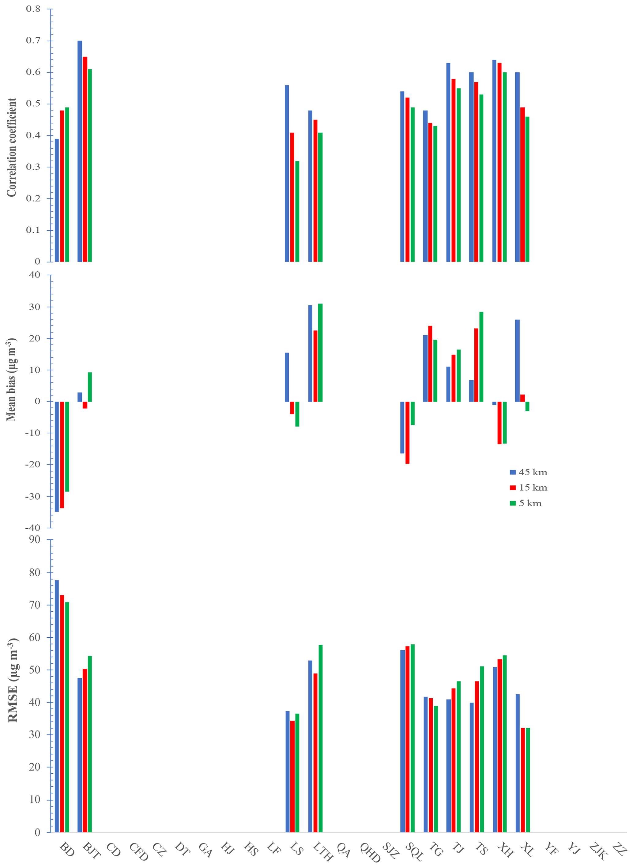
Figure 4Comparisons of MB, RMSE, and correlation coefficient r of surface PM2.5 from different horizontal resolutions at each air quality monitoring site (blank space indicates no data are available) for the year of 2010.
At the individual site level, the impact of grid resolution on surface NOx and CO (figures not shown) modeling was similar to that at the regional average. Finer-resolution simulation generally reduced MB and RMSE. The results of the 45 km grid always had the largest bias. The underestimates of NOx at least partially explained the overestimate of surface O3 at each site due to a less efficient NO titration of O3. This suggested that a higher-resolution modeling with more accurate spatial representation of NOx emissions would help improve its performance on surface O3 simulations.
The signals for SO2 and PM10 (figures not shown) simulations were mixed as well. For example, the largest bias for SO2 simulation over sites BD, CZ, GA, HS, LS, QA, QHD, XH, XL, YF, and YJ occurred when applying the 45 km grid, while the maximum bias over BJT, DT, HJ, LF, LTH, SJZ, SQL, TG, TJ, TS, ZJK, and ZZ happened at the 5 km resolution. Sites CD and CFD saw the largest bias at the 15 km resolution. Unlike PM10 which was almost always underestimated at each site regardless of grid resolution, SO2 was overestimated at 18 out of 25 sites and underestimated at the remaining 7 sites.
An effort has been made to identify the potential reasons that caused the model–observation discrepancy. First and as discussed previously, the spatial distribution of emissions was one key to determining air quality forecast accuracy. Figure S3 shows the typical time evolutions of surface O3 and NOx over rural (XL) and urban (QHD) sites. It can readily be seen that NOx was underestimated at the urban site but overestimated at the rural site. The coarser the grid resolution was, the severer the underestimates and overestimates were. This indicated that the 45 km resolution tended to smooth out emissions to make urban sites (or emission centers) less polluted but rural sites more polluted. This in turn led to an overestimate of surface O3 over the urban sites mainly due to the reduced NOx titration effect, especially at night when there was no photochemical O3 formation. The statistics showed that the bias of the modeled daytime (08:00–18:00 LT) average surface O3 was 30 %–90 % smaller than that of the daily average in the urban sites, no matter which grid resolution was applied. This suggested that in the future the high-resolution emissions, especially proper representation of emission gradients, would be helpful in improving air quality prediction. The effect of emission gradients associated with the grid resolution will be further discussed in the inter-resolution comparisons section.
Next, the driving meteorology, especially wind, was important for accurately forecasting air quality over coastal areas that bore sharp thermal contrasts. The QHD site is located approximately 5 km from the ocean and is subject to sea breeze effects. The detailed analysis of meteorology and air quality over QHD was conducted. The results indicated that the choice of grid resolution had large impacts on model simulations at this coastal site. The selection of the 5 km grid reduced biases of both surface temperature and wind speed. The biases of temperature reduced from 1.22 K (45 km) to −0.42 K (15 km) and further down to −0.31 K when the 5 km grid was applied. The biases of surface wind speed for the 45, 15, and 5 km grids were 3.72, 4.19, and 1.95 m s−1, respectively. The improvement of meteorology forecasts helped reduce the biases of air quality modeling. The biases of O3∕NOx for the 45, 15, and 5 km resolution grids were , , and ppbv, respectively. The improvement using the 15 km grid over the 45 km grid was remarkable but that using the 5 km grid over the 15 km grid was marginal. The result emphasized the importance of high-resolution modeling to improvements in air quality forecast skills, especially in coastal and complex-terrain areas (e.g., QHD and XL).
(c) Extreme values
High concentrations of air pollutants are of more concern because of their adverse health effects on both human beings and ecosystems. High pollutant concentrations also pose a greater risk for noncompliance to the ambient air quality standards. Therefore, evaluations of impacts of grid resolution on extreme concentrations of air pollutants are desirable.
Figure 5 displays the probability density function distributions of six pollutants based on hourly surface concentrations across the monitoring sites. This analysis was focused on high pollutant concentrations with the cutoff values for CO, O3, NOx, SO2, PM2.5, and PM10 being 1.1 ppmv, 60 ppbv, 25 ppbv, 5.5 ppbv, 15 µg m−3, and 30 µg m−3, respectively. It appeared that NU-WRF, regardless of the grid resolutions, failed to simulate surface CO with concentrations of more than 4 ppmv, likely due to the underestimate of CO emissions (Kong et al., 2020). The grid resolution appeared to have limited impact on surface PM10 simulations when PM10 concentrations were more than 200 µg m−3. On the other hand, the grid resolution had a large impact on NU-WRF's capability to simulate high surface concentrations of O3, NOx, SO2, and PM2.5. For surface O3 with concentrations of more than 100 ppbv, the NU-WRF results with the 5 km grid appeared to better agree with the probability distribution of observations. For surface NOx with concentrations of more than 70 ppbv, the NU-WRF results with the 5 km resolution grid better mimicked the observed distribution. Modeling with the 5 km grid also yielded the best results of distributions, in comparison to the respective observations, of SO2 with concentrations of more than 45 ppbv and of PM2.5 with concentrations greater than 120 µg m−3.
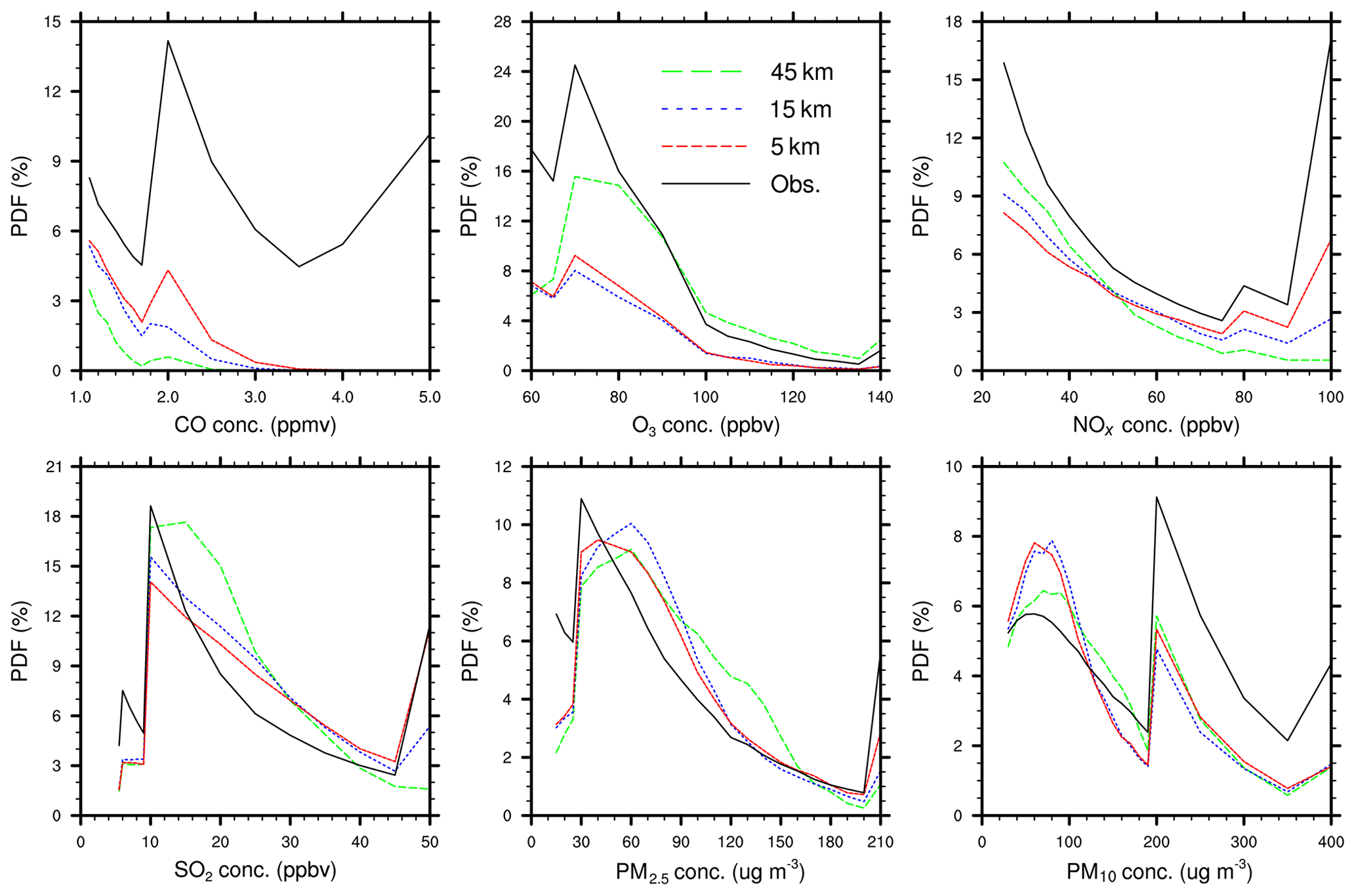
Figure 5Probability density function (PDF) plots for hourly concentrations of surface air quality for the year of 2010.
Table 2 lists the occurrences of violations of China's national ambient air quality standards (NAAQSs) for the six pollutants from both observations and simulations in which columns Class 1 and Class 2 list the standards for rural and urban–suburban sites, respectively, and column Frequency indicates the time integration of each NAAQS. It was apparent that NU-WRF failed to report CO violations at any grid resolutions. No CO NAAQS violation was simulated, but the observation showed that surface CO exceeded the national standard more than 1000 times. NU-WRF underestimated the NAAQS exceedances of NOx and SO2. A higher-resolution grid appeared to be able to catch more violations although the modeled results at the 5 km resolution only captured 33 % and 10 % of the observed exceedances of NOx and SO2, respectively. NU-WRF overestimated surface O3 and PM2.5 when their concentrations were more than the corresponding NAAQS. The fine grid resolution (i.e., 5 km) appeared to largely reduce the overestimation of surface O3 exceedances as compared to the 45 km grid but only marginally compared to the 15 km grid. Compared to the number of observed occurrences of surface O3 standard violation (3684), the simulated exceedances were 5.7, 1.8, and 1.7 times higher when employing the 45, 15, and 5 km resolution grid, respectively. The observations showed 1343 occurrences of surface PM2.5 exceedances, while the modeled exceedances were 377, 267, and 231 more for the 45, 15, and 5 km grids, respectively. As for surface PM10, the modeled exceedances were approximately 27 %, 43 %, and 41 % less than the observed ones for the 45, 15, and 5 km grids, respectively.
Table 2Comparison of occurrences of exceedances of China's national ambient air quality standards between observations (Obs.) and simulations.
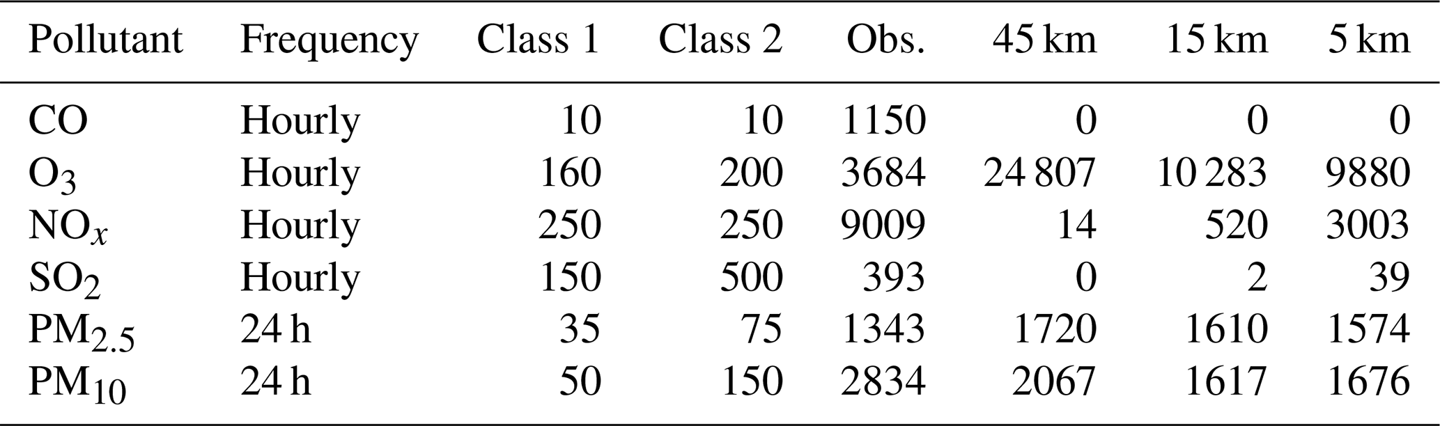
Class 1/2 standards are for rural/suburban–urban, respectively. Units are ppbm for CO; ppbv for O3, NOx, and SO2; and µg m−3 for PM2.5 and PM10.
3.2 Inter-resolution comparisons
It is informative to compare the NU-WRF results of different horizontal resolutions. This, in addition to the discussion in Sect. 3.1.2b, can help us understand the reasons why model resolution matters.
3.2.1 Emissions
There were two types of emissions applied in this study. One was the prescribed emissions of anthropogenic and wildfire sources and the other was emissions computed online using real-time meteorology (or dynamic emissions) including emissions from biogenic sources, dust sources, and sea spray. Amounts of and temporal variations in dynamic emissions depended on surrounding environmental conditions. For example, air temperature and solar radiation regulate biogenic emissions (Guenther et al., 2006). Surface wind speed plays a major role in both dust (Ginoux et al., 2001; Chin et al., 2002) and sea salt emissions (Gong, 2003).
For the prescribed emissions, the differences in domain total mass of each grid were small (less than 5 %). However, the emission gradient around sources of a fine-resolution grid appeared to be sharper than that of a coarse-resolution grid. This meant that a coarse grid tended to distribute the prescribed emissions more evenly into the domain, while a fine grid tended to produce more extreme concentrations of primary pollutants (emitted directly from a source) such as NOx and SO2, as shown in Table 2.
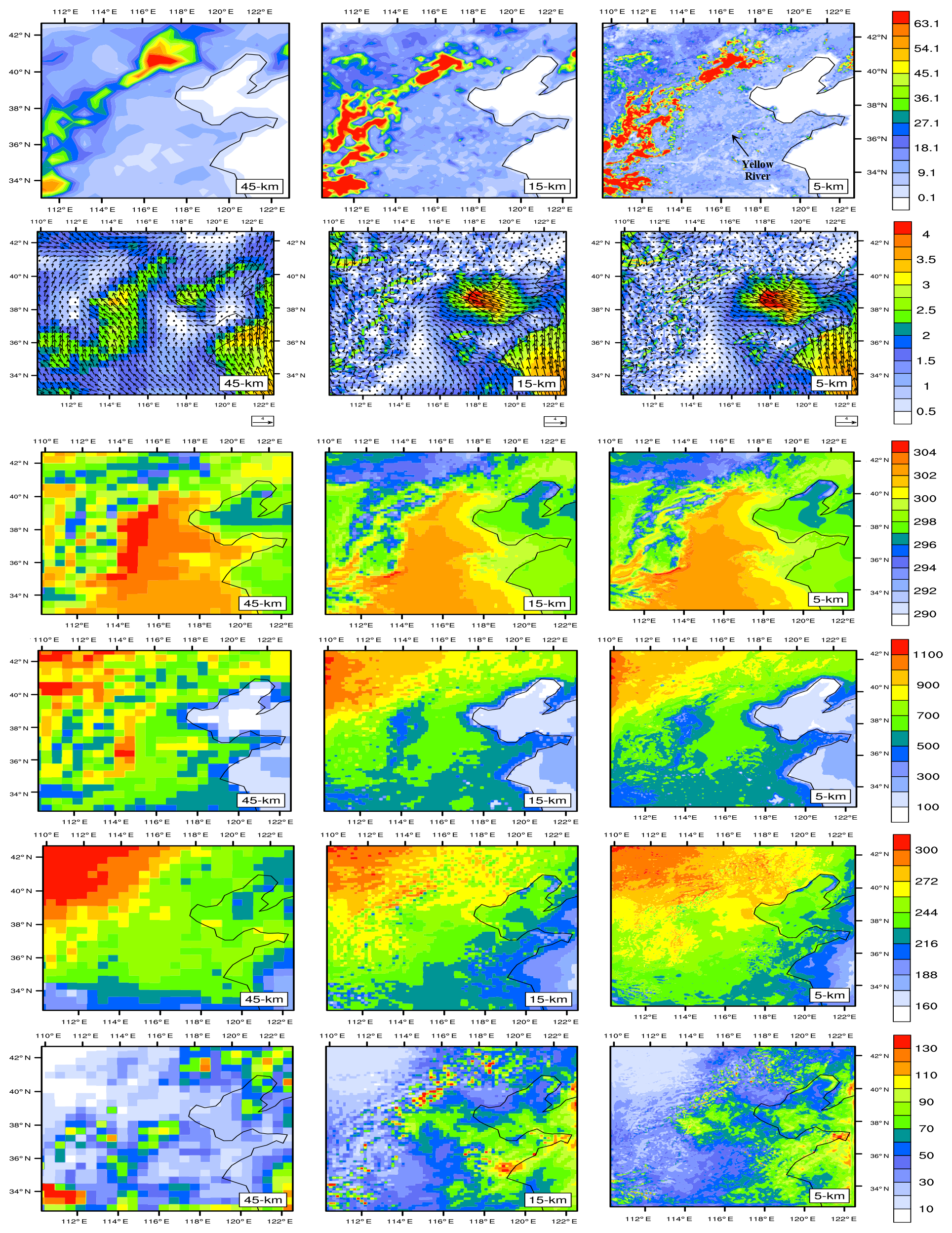
Figure 6Simulated emissions and July average meteorology from the three grids: first row is isoprene emissions (mol km−2 h−1) from biogenic sources on a typical summer day; second row is surface wind vector with the shading representing wind speed (m s−1); third row is surface air temperature (K); fourth row is PBLH (m); fifth row is SWDOWN (W m−2); sixth row is CWP (g m−2).
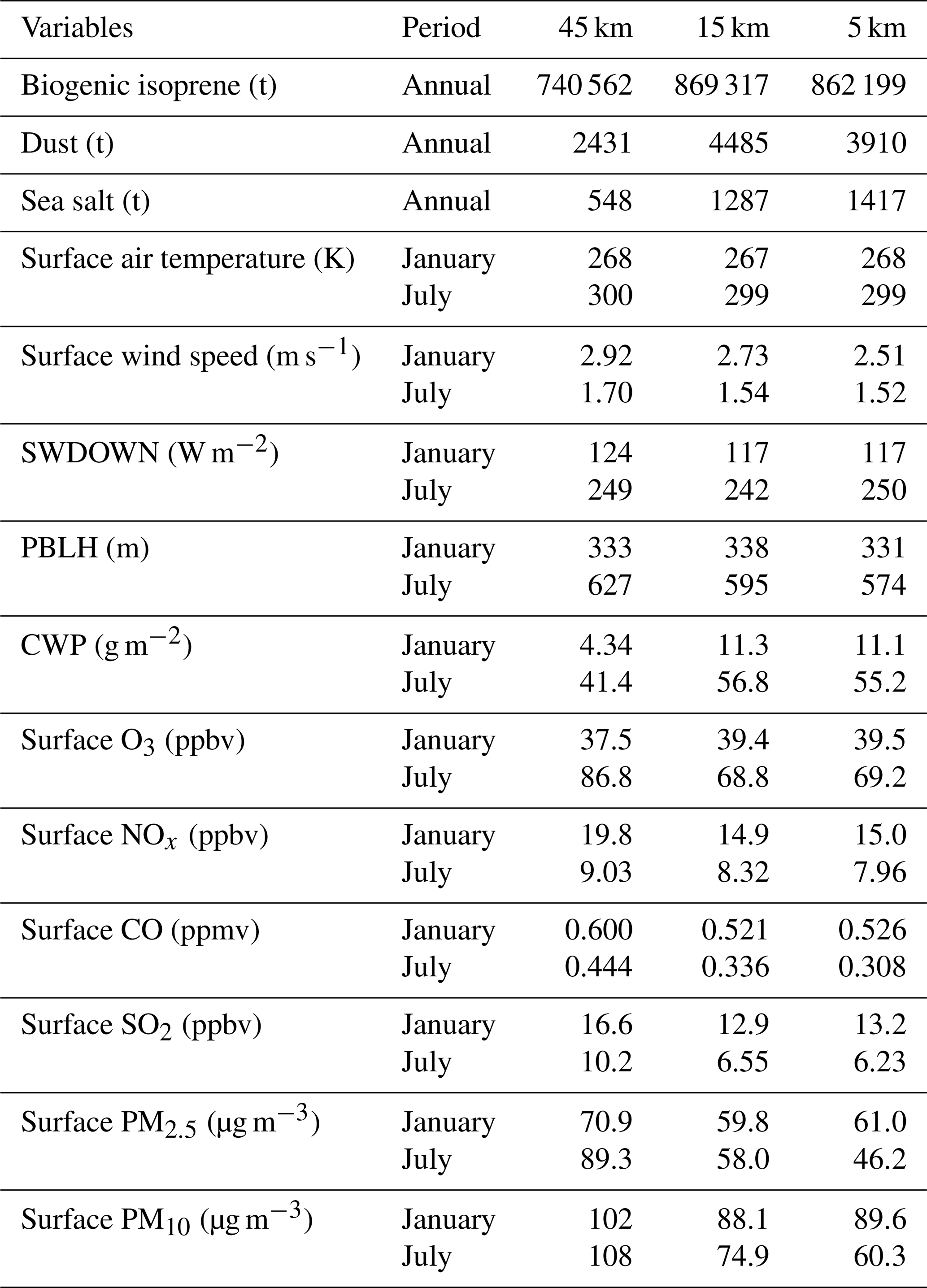
Online-calculated emissions, on the other hand, displayed large differences in both gradient and total mass. Similar to the case of prescribed emissions, a fine-resolution grid tended to give a sharper gradient of dynamic emissions than a coarse-resolution grid did, as highlighted in Fig. 6 (first row), which illustrated the biogenic isoprene emissions (mol km−2 h−1) on a typical summer day. It was apparent that many more details were simulated using a fine-resolution grid, so the flow of the Yellow River can even be seen on the 5 km resolution map that was otherwise invisible on the coarser-resolution maps. Meanwhile, the total masses of dynamic emissions showed large differences across different-resolution grids as listed in Table 3. On an annual basis, the domain total isoprene emissions were 740 562 t when estimated using the 45 km grid, which is approximately 85 % and 86 % of those estimated with the 15 and 5 km grids, respectively. The total dust emissions of the 45 km grid were 2431 t, which is only 54 % and 62 % of those based on the respective 15 and 5 km grids. The percentage contrasts for sea salt emissions were even larger, with emissions of the 15 and 5 km grids being 1.3 and 1.6 times more, respectively, than those of the 45 km grid. It should be noted that, although they differed greatly between the 45 and 15 km grids, the dynamic emissions of the 5 km grid were much closer to those of the 15 km grid, partially explaining why the impact of model resolution on surface air quality was less remarkable when increasing the resolution from 15 to 5 km than from 45 to 15 km.
Table 3Domain total emissions and average meteorology and air quality at various resolutions.
The spatial (gradient) and mass variations in emissions of different-resolution grids result in differences in air quality simulations.
3.2.2 Meteorology
It has been reported that simulated meteorology varies in response to selections of model grid resolutions (e.g., Tie et al., 2010; Lee et al., 2018). Meteorology plays an important role in regulating regional air quality: it affects the emissions amount originating from biogenic, dust, and sea sources; it impacts atmospheric chemical and photochemical transformation; and it directs air flows and the associated transport of trace gases and aerosols. In this investigation, a few meteorological parameters key to air pollutant generation and accumulation were analyzed, including surface wind, air temperature, downward shortwave flux at surface (SWDOWN), planetary boundary layer height (PBLH), and cloud water (liquid + ice) path (CWP). We focused on months that were prone to deteriorated PM2.5 (January) and O3 (July) air quality as shown in Fig. 6 and Table 3.
NU-WRF simulated a similar direction of surface wind in July 2010 over the eastern portion of the domain (second row of Fig. 6). In general, average wind speed was higher over the Bohai Sea and Yellow Sea than over the surrounding land areas, with the dominating wind direction being south and southeast. Based on the results from the 15 and 5 km grids, the peak average wind speeds of over 4 m s−1 were found in Bohai Bay blowing toward Tianjin and Beijing. However, such a peak was absent from the 45 km grid simulation. In the west portion of the domain, the wind direction generally changed from southeast in the south to southwest in the north. Compared to the more organized wind directions of the 45 km grid, wind directions of the 15 and 5 km grids were more chaotic. Averaged over the domain, the January mean wind speed of the 45 km grid was 2.92 m s−1, which was 7 % and 16 % higher than those of the 15 and 5 km grids, respectively. The highest July mean wind speed was again simulated with the 45 km grid; it was 10 % and 12 % higher than the corresponding wind speed of the 15 and 5 km grids, respectively.
Overall, NU-WRF simulated very similar magnitudes and spatial patterns of surface air temperature in July (third row of Fig. 6), regardless of the selection of grid resolution. Large portions of the NCP experienced July average air temperatures of more than 300 K. The minimum average temperature of approximately 290 K was found in the central northern part of the domain, which was part of the Mongolian Plateau with elevations being over 1500 m a.s.l. (meters above sea level). The domain average January and July surface air temperatures were around 268 and 300 K, respectively, for simulations of all three grids.
As expected, the modeling results from all three grids (fourth row of Fig. 6) showed that July average PBLH over sea was much smaller than that over land. The largest average PBLH (more than 1000 m) was found in the northwestern corner of the domain with a dominant land cover type of grassland mosaicked with open shrubland that appeared to be drier than the other land cover types in the domain. The high sensible heating associated with dry soil tended to produce the deep PBL (planetary boundary layer; Tao et al., 2013). The largest domain average PBLHs in January and July were found in the simulations of the 15 and 45 km grids, respectively. In January, the differences of the domain average PBLHs from different grid resolutions were small and within 2 % of each other. In July, however, such differences can be over 9 %.
Regardless of the grid resolutions, NU-WRF simulated a generally southeast–northwest gradient of SWDOWN in July with the highest flux (over 300 W m−2) occurring in the northwestern domain (fifth row of Fig. 6). The differences between the maximum and minimum domain average SWDOWN of the three grids were 5.6 % and 3.3 % in January and July, respectively.
CWP represented the vertical integration of cloud water (including both liquid and ice phases) contents and can be regarded as a proxy of cloud amount and coverage. Opposite to the SWDOWN case, NU-WRF modeled a generally northwest–southeast gradient of CWP in July with the highest values found in the southeastern domain (sixth row of Fig. 6). This is understandable since cloud reflects and scatters the incoming solar radiation and thus affects SWDOWN. Large cloud existence tended to reduce the solar flux reaching the Earth's surface underneath. The CWP differences among the model results of different grid resolutions appeared to be larger than SWDOWN differences. In July, the domain average CWPs of the 15 and 5 km grids were 37 % and 33 % larger than that of the 45 km grid, respectively. The gaps were even larger in January, during which the domain average CWPs from the 15 and 5 km grids were approximately 1.6 times larger than that from the 45 km grid.
3.2.3 Air quality
In response to the aforementioned emissions and meteorological variations resulting from the selection of model grid resolutions, changes in regional air quality ensued as illustrated in Fig. 7 and Table 3. Figure 7 shows the July average concentrations of ground-level O3 and its precursors of NOx and CO, as well as the January mean concentrations of surface SO2, PM2.5, and PM10, during which month the respective pollutants tended to reach high concentrations.
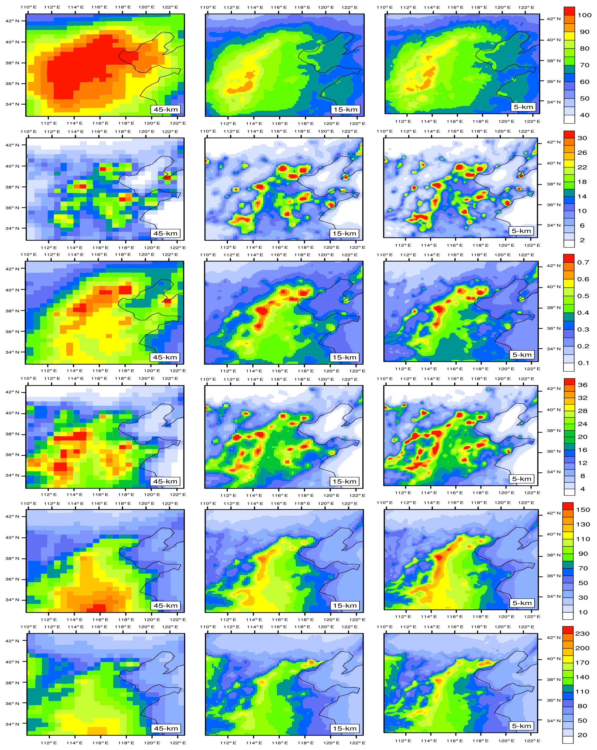
Figure 7Simulated January (SO2, PM2.5, and PM10) and July (O3, NOx, and CO) surface average air quality from the three grids: first row is O3 (ppbv); second row is NOx (ppbv); third row is CO (ppmv); fourth row is SO2 (ppbv); fifth row is PM2.5 (µg m−3); sixth row is PM10 (µg m−3).
O3 is a secondary pollutant that is formed in the atmosphere through complex photochemical processes upon its precursors such as NOx and volatile organic compounds (VOCs). Figure 7 (row 1) shows that the spatial distributions of surface O3 are similar to each other but the concentrations of the 15 and 5 km grids are smaller than those from the 45 km grid. The domain average surface O3 concentration in July was approximately 87 ppbv based on the results from the 45 km grid, which was 26 % and 25 % higher than those of the 15 and 5 km grids, respectively. In January, however, the highest domain average concentration occurred when the 5 km grid was used, which was 5.3 % higher than that of the 45 km grid.
For the primary pollutants, i.e., NOx, CO, and SO2 (rows 2–4 of Fig. 7, respectively), which were emitted directly by their sources, the spatial distributions of their concentrations mimicked closely their emission distributions. High concentrations centered around emission sources with a reducing gradient outward. The domain average concentrations of these three pollutants of the 45 km grid results were always the largest in both January and July. The average surface NOx concentrations from the simulations of the 15 and 5 km grids were around 24 % lower than their counterpart of the 45 km grid in January. In July, the differences were reduced to 7.9 % and 11.8 % for the 15 and 5 km grids, respectively. On the other hand, the larger percentage differences, as compared to the results of the 45 km grid, occurred in July rather than in January for both CO and SO2. For example, the surface CO concentrations of the 5 km grid were 12.3 % and 30.6 % lower than those based on the 45 km grid in January and July, respectively. The ground-level SO2 concentrations from the 5 km grid were 20.5 % and 38.9 lower than those from the 45 km grid in January and July, respectively.
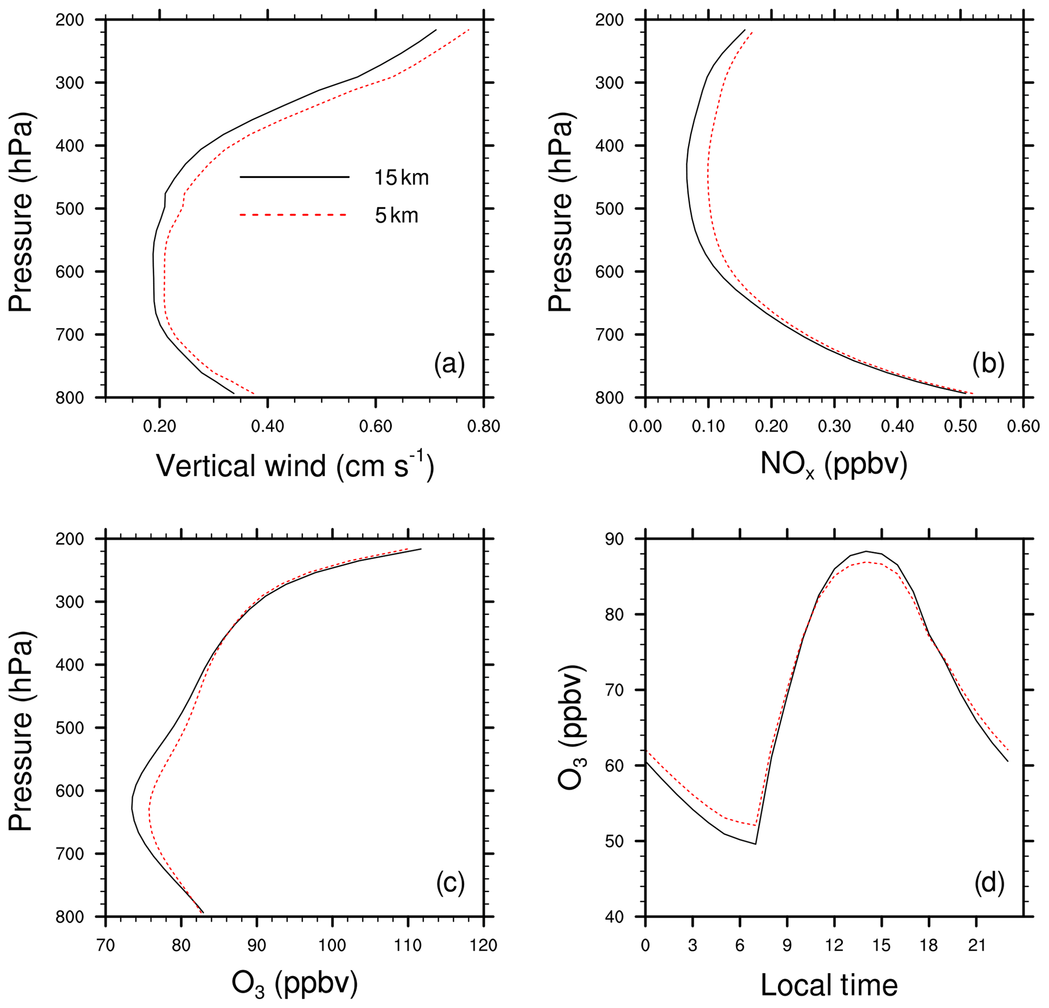
Figure 8Domain average profiles of vertical wind, NOx, and O3 concentrations (a–c) and domain average diurnal variations in surface O3 over July (d).
It was interesting to note that, among the three cases, the domain average July surface O3 and NOx concentrations were both the highest from the 45 km grid, contrary to the results discussed in Sect. 3.1.2a, where the highest O3 concentration occurred in the simulation using the 45 km grid and the highest NOx concentration happened with the 5 km grid. This seemingly contradictory result was internally consistent. Section 3.1.2a actually depicted the average surface concentrations in an urban environment (23 of 25 monitoring sites were in an urban–suburban setting), where surface O3 formation was typically VOC controlled such that NO tended to consume O3 through titrations. As discussed in Sect. 3.2.1, a 5 km grid gave a much sharper emission gradient with anthropogenic emissions concentrating in urban–suburban areas. This led to higher NOx concentrations around urban–suburban areas in the simulation with the 5 km grid, which effectively resulted in lower O3 concentrations there through the NO titration effect. The domain average discussed in this section, however, was the average covering the vast rural area that was generally NOx-limited such that surface O3 formation was controlled by the availability of NOx, with more NOx resulting in more O3 through photochemical processes. In this case, the 45 km grid tended to distribute NOx emissions more evenly across the region, effectively decreasing the surface NOx concentration in urban areas but increasing it over rural areas. The larger average July wind speed simulated by the 45 km grid (Fig. 6 and Table 3) further smoothed out the NOx distribution in the NCP. This in turn increased the domain average surface O3 concentration via photochemistry based on the 45 km resolution results. In addition, vertical lifting played an important role in explaining the maximum regional O3 in July simulated by the 45 km grid as compared to the results by the other two grid resolutions. As displayed in Fig. S4, a fine-resolution model (e.g., 5 km) tended to produce a stronger updraft than a coarse-resolution model (e.g., 45 km), consistent with the findings by Lee et al. (2018). The strong uplift would bring more surface pollutants such as NOx into the upper atmosphere, thus further reducing the NOx availability at ground and limiting the surface ozone production but increasing its formation in the upper atmosphere.
Vertical distributions of O3 also tend to have a sizable impact on the next day's surface O3 levels (e.g., Kuang et al., 2011; Caputi et al., 2019). Figure 8 illustrates the domain average profiles of vertical wind, NOx, O3 (panels a–c), and the average diurnal distribution of surface O3 (panel d) over July. Here we limited our discussion to the results from the 15 and 5 km grids since the 45 km grid artificially allowed more NOx emissions to spread to rural areas to produce much more O3, as shown in the previous paragraph. Lee et al. (2018) claimed that a coarse-resolution model appeared to lower updraft as compared with a fine-resolution model. This study agreed with their finding, as illustrated in Fig. 8a. The domain average July vertical wind in the simulation with the 5 km grid ranged from 0.25 to 0.45 cm s−1 (upward) between 800 and 400 hPa, stronger than the corresponding one of the 15 km grid. The reason was complex and the aerosol–cloud-interaction-induced freezing–evaporation-related invigoration mechanism played a role (Lee et al., 2018). The stronger upward wind tended to lift more gaseous pollutants up to the free troposphere as shown in Fig. 8b (NOx) and Fig. 8c (O3). The pollutants there would have visible impacts on the following-day surface air quality, especially on O3 levels at night and in the morning when sunlight breaks through the nocturnal planetary boundary layer, as evidenced in Fig. 8d. At night with no photochemical formation, surface O3 concentration was largely controlled by upper-level O3 mixing down, NO titration, and O3 dry deposition. With virtually the same average surface NO concentrations from the 15 and 5 km grids, the upper-level O3 mixing down appeared to control the relative magnitudes of surface O3 concentrations simulated using the 15 and 5 km grids. This partially explained why, at night and in the early morning, the ground-level O3 concentrations were higher in the 5 km grid than the 15 km grid. During the daytime when the photochemical formation of O3 takes control, the regional average surface O3 concentrations are largely determined by the availability of O3 precursors (i.e., NOx and VOC) and ambient environmental conditions. In this case, more spreading NOx emissions of the 15 km grid appeared to generate more surface O3 than the 5 km grid did.
PM2.5 and PM10 were mixed pollutants that not only were emitted by various sources but also were generated in the atmosphere through physical and chemical processes. Figure 7 shows that high surface concentrations of PM2.5 (more than 120 µg m−3, row 5) and of PM10 (more than 170 µg m−3, row 6) were still found around the source areas based on the modeling results of the 15 and 5 km grids. However, high PM2.5 and PM10 concentrations spread out to larger areas based on the results from the 45 km grid as compared to the ones from the finer grid resolutions. Similar to the primary pollutants, the largest domain average surface concentrations occurred when a 45 km grid was used for the NU-WRF simulation. The domain average PM2.5 concentrations of the 15 and 5 km grids in January were 15.7 % and 14 % lower than those from the 45 km grid, respectively. The surface PM2.5 concentration differences among the results of different grid resolutions grew larger in July, reaching 48 % when comparing the result from the 5 km grid to that from the 45 km grid. The domain average surface PM10 concentrations showed a similar pattern to that of PM2.5, with the results from the 5 km grid being 12.2 % (January) and 44.2 % (July) smaller than that from the 45 km grid.
It is worth noting that the magnitudes and spatial distributions of ground-level pollutants were close to each other when comparing the results of the 15 and 5 km grids. This again indicates that the improvement of fine-grid-resolution modeling reduces at a certain point. In future MICS-Asia efforts, a 15 km grid appears to offer the optimized results balanced between performance and resources.
Contributing to MICS-Asia Phase III, whose goals included identifying and reducing air quality modeling uncertainty over the region, this investigation examined the impact of model grid resolutions on the performances of meteorology and air quality simulation. To achieve this, NU-WRF was employed to simulate 2010 air quality over the NCP region with three grid resolutions of 45, 15, and 5 km. The modeling results were compared to the observations of surface meteorology archived by CMA and of ground-level air quality collected via CERN. The intermodel comparison among the simulation results of the three grids was also conducted to understand the reasons why model resolution mattered.
The analysis showed that there was no single resolution which would yield the best reproduction of meteorology and air quality across all monitoring sites. From a regional average prospective (i.e., across all monitoring sites in this study), the choice of grid resolution appeared to have a minimal influence on air temperature modeling but affected wind, RH, and precipitation simulation profoundly. A 5 km grid appeared to give the best wind simulation as compared to the observations, quantified by bias, RMSE, standard deviation, and correlation. Compared to the one from the 45 km grid, the simulated wind speed from the 5 km grid reduced the positive bias by 46.8 %. While a 15 km grid yielded the best overall performance of RH modeling, the result of the 45 km grid gave the most realistic reproduction of precipitation. The statement on precipitation should be taken with caution since it was based on comparison with the site observations. Bearing in mind the very heterogeneous nature of precipitation, the penalty of the model hitting or missing a rain event was severe. Thus, the coarse grid covering more areas within a grid cell would reduce chances of mistaken precipitation hitting or missing simulations. However, a comparison of modeled precipitation to gridded observations that were reconstructed using the synergraphic mapping algorithm with topographic adjustment to the monthly precipitation climatology showed the opposite result, where the fine-resolution modeling showed superior reproduction of precipitation than the coarse-resolution simulation did (Gao et al., 2017).
The simulated meteorology differences due to the selection of grid resolution would consequently lead to differences in air quality simulation. Air pollutant concentrations were basically determined by their emissions and underlying meteorology that directed their formation (e.g., O3 and aerosols), transport, and removal processes. For the prescribed emissions originating from anthropogenic and wildfire sources, the grid resolution had limited influence on emissions amount – less than 5 % difference with each other under the different-resolution grids – but a large impact on emission spatial distribution, with sharper emission gradients around sources from a fine-resolution grid than from a coarse-resolution one. For the dynamic emissions driven by meteorology, not only was an emission gradient around a source larger from a higher-resolution grid but also the total emissions amount varied greatly. For example, the domain total annual biogenic isoprene emissions from a 5 km grid was about 16 % larger than those from a 45 km grid due to the underlying differences in land cover and meteorology.
Though the impact of grid resolution on air quality varied from location to location, a finer grid yielded better results for daily mean surface O3, NOx, CO, and PM2.5 simulations from a regional average perspective. For example, after reducing the grid resolution from 45 to 15 km, the positive bias of daily mean surface O3 and PM2.5 decreased by 15 % and 75 %, respectively. Fine-resolution modeling was especially beneficial to high pollutant concentration forecasting. This was important to air quality management. Taking China's NAAQSs as cutoff values for each pollutant, the frequencies of noncompliant occurrences of O3, NOx, SO2, and PM2.5 in the 5 km grid simulation were much closer to the observations than those of the 45 km modeling. For example, the simulation with the 5 km grid produced 168 % and 17 % more exceedances of the NAAQSs of O3 and PM2.5, respectively, whereas the respective exceedances were 573 % and 28 % more with modeling using the 45 km grid, as compared to the observed exceedances. It also was worth noting that the benefit of increasing grid resolution to better surface O3 and PM2.5 simulations started to diminish when the horizontal resolution reached 15 km, agreeing with the finding by Valari and Menut (2008). There was a caveat, though. The anthropogenic MIX and fire GFEDv3 emissions inventories bore 0.25∘ by 0.25∘ and 0.5∘ by 0.5∘ resolutions, respectively. These resolutions cannot resolve the 5 km grid. Should a 5 km resolution emissions inventory be available and used, the benefit of high-resolution modeling would likely be more prominent.
It should be pointed out that NU-WRF significantly overestimated surface O3 concentration but underestimated ground-level CO and NOx concentrations regardless of grid resolutions. This was true not only for the regional averages but also at the majority of the monitoring sites. Missing emissions were believed to be largely responsible for this result (Kong et al., 2020). Underestimate of surface NOx tended to increase ground-level O3 due to the reduced titration effect, especially at night over urban areas that were typically NOx abundant.
In conclusion, grid resolution had a profound effect on NU-WRF performance on meteorology and air quality over East Asia. A fine-resolution grid did not always generate the best modeling results, and the proper selection of horizontal resolution hinged on investigation topics for a given set of physics and chemistry choices in a model. With regard to MICS-Asia Phase III, whose major goal was to examine regional air quality, in general, the finer the grid resolution was, the better the simulation results would be. This was especially true over the coastal areas and complex terrains where a sharp local energy gradient existed. A fine-resolution grid was also extremely helpful in reproducing pollutants at higher concentrations that were most relevant to air quality planning and management. However, the benefit of high resolution was not linear with the decrease in grid size. At a certain point, the improved modeling accuracy due to an increase in grid resolution was so marginal that it could not justify the computational cost associated with the fine-grid simulation. Based on the balance of modeling accuracy and efficiency, a 15 km horizontal grid appeared to be an appropriate choice to optimize model performance and resource usage if the study domain were to remain unchanged for future MICS-Asia activities. The study suggested that the high-resolution emissions, especially the proper representation of emission gradients, would be helpful in improving air quality prediction. Moreover, the profile measurements of both meteorology and air quality, in conjunction with the ground monitoring networks, would be greatly helpful in identifying model deficiencies and thus improving model forecast skills.
All data collected and generated for this research are archived and stored on NASA Center for Climate Simulation (NCCS) servers. Due to the sheer extent of data, it is impractical to upload data to a public domain repository. However, the authors will be happy to share data on an individual-request basis.
The supplement related to this article is available online at: https://doi.org/10.5194/acp-20-2319-2020-supplement.
ZT and MC designed the experiments. ZT, MG, TK, DK, and HB carried out the experiments, working on various modeling components. YW and ZL collected, organized, and archived the ground air quality measurement data. All authors contributed to model result analysis and interpretation. ZT prepared the paper with contributions from all coauthors.
The authors declare that they have no conflict of interest.
This article is part of the special issue “Regional assessment of air pollution and climate change over East and Southeast Asia: results from MICS-Asia Phase III”. It is not associated with a conference.
This work was supported by the NASA's Atmospheric Composition Modeling and Analysis Program (ACMAP) and Modeling, Analysis, and Prediction (MAP) program. The authors thank MICS-Asia for its organized platform of discussion and data sharing. This work was not possible without the supercomputing and mass storage support of the NCCS.
This research has partially been supported by NASA (grant no. NNH14ZDA001N-ACMAP).
This paper was edited by Hailong Wang and reviewed by two anonymous referees.
Akimoto, H., Mori, Y., Sasaki, K., Nakanishi, H., Ohizumi, T., and Itano, Y.: Analysis of monitoring data of ground-level ozone in Japan for long-term trend during 1990–2010: Causes of temporal and spatial variation, Atmos. Environ., 102, 302–310, 2015.
Anenberg, S. C., Horowitz, L. W., Tong, D. Q., and West J. J.: An estimate of the global burden of anthropogenic ozone and fine particulate matter on premature human mortality using atmospheric modeling, Environ. Health Perspect., 118, 1189–1195, https://doi.org/10.1289/ehp.0901220, 2010.
Cai, W., Li, K., Liao, H., Wang, H., and Wu, L.: Weather conditions conductive to Beijing severe haze more frequent under climate change, Nat. Clim. Change, 7, 257–263, https://doi.org/10.1038/NCLIMAE3249, 2017.
Caputi, D. J., Faloona, I., Trousdell, J., Smoot, J., Falk, N., and Conley, S.: Residual layer ozone, mixing, and the nocturnal jet in California's San Joaquin Valley, Atmos. Chem. Phys., 19, 4721–4740, https://doi.org/10.5194/acp-19-4721-2019, 2019.
Carmichael, G., Calori, G., Hayami, H., Uno, I., Cho, S. Y., Engardt, M., Kim, S. B., Ichikawa, Y., Ikeda, Y., Woo, J. H., Ueda, H., and Amann, M.: The MICS-Asia study: model intercomparison of long-range transport and sulfur deposition in East Asia, Atmos. Environ., 36, 175–199, https://doi.org/10.1016/s1352-2310(01)00448-4, 2002.
Carmichael, G., Sakurai, T., Streets, D., Hozumi, Y., Ueda, H., Park, S., Fung, C., Han, Z., Kajino, M., and Engardt, M.: MICS-Asia II: The model intercomparison study for Asia Phase II: methodology and overview of findings, Atmos. Environ., 42, 3468–3490, https://doi.org/10.1016/j.atmosenv.2007.04.007, 2008.
Chen, L., Gao, Y., Zhang, M., Fu, J. S., Zhu, J., Liao, H., Li, J., Huang, K., Ge, B., Wang, X., Lam, Y. F., Lin, C.-Y., Itahashi, S., Nagashima, T., Kajino, M., Yamaji, K., Wang, Z., and Kurokawa, J.: MICS-Asia III: multi-model comparison and evaluation of aerosol over East Asia, Atmos. Chem. Phys., 19, 11911–11937, https://doi.org/10.5194/acp-19-11911-2019, 2019.
Chin, M., Ginoux, P., Kinne, S., Torres, O., Holben, B. N., Duncan, B. N., Martin, R. V., Logan, J. A., Higurashi, A., and Nakajima, T.: Tropospheric aerosol optical thickness from the GOCART model and comparisons with satellite and Sun photometer measurements, J. Atmos. Sci., 59, 461–483, 2002.
Chin, M., Diehl, T., Ginoux, P., and Malm, W.: Intercontinental transport of pollution and dust aerosols: implications for regional air quality, Atmos. Chem. Phys., 7, 5501–5517, https://doi.org/10.5194/acp-7-5501-2007, 2007.
Chou, M.-D. and Suarez, M. J.: A solar radiation parameterization (CLIRAD-SW) for atmospheric studies, vol. 15, NASA Tech. Rep. NASA/TM-1999-10460, NASA, Greenbelt, Maryland, USA, 38 pp., 1999.
Ek, M. B., Mitchell, K. E., Lin, Y., Rogers, E., Grunmann, P., Koren, V., Gayno, G., and Tarpley, J. D.: Implementation of Noah land surface model advances in the National Centers for Environmental Prediction operational mesoscale Eta Model, J. Geophys. Res., 108, 8851, https://doi.org/10.1029/2002JD003296, 2003.
Emmons, L. K., Walters, S., Hess, P. G., Lamarque, J.-F., Pfister, G. G., Fillmore, D., Granier, C., Guenther, A., Kinnison, D., Laepple, T., Orlando, J., Tie, X., Tyndall, G., Wiedinmyer, C., Baughcum, S. L., and Kloster, S.: Description and evaluation of the Model for Ozone and Related chemical Tracers, version 4 (MOZART-4), Geosci. Model Dev., 3, 43–67, https://doi.org/10.5194/gmd-3-43-2010, 2010.
Gao, M., Carmichael, G. R., Wang, Y., Saide, P. E., Yu, M., Xin, J., Liu, Z., and Wang, Z.: Modeling study of the 2010 regional haze event in the North China Plain, Atmos. Chem. Phys., 16, 1673–1691, https://doi.org/10.5194/acp-16-1673-2016, 2016.
Gao, M., Han, Z., Liu, Z., Li, M., Xin, J., Tao, Z., Li, J., Kang, J.-E., Huang, K., Dong, X., Zhuang, B., Li, S., Ge, B., Wu, Q., Cheng, Y., Wang, Y., Lee, H.-J., Kim, C.-H., Fu, J. S., Wang, T., Chin, M., Woo, J.-H., Zhang, Q., Wang, Z., and Carmichael, G. R.: Air quality and climate change, Topic 3 of the Model Inter-Comparison Study for Asia Phase III (MICS-Asia III) – Part 1: Overview and model evaluation, Atmos. Chem. Phys., 18, 4859–4884, https://doi.org/10.5194/acp-18-4859-2018, 2018.
Gao, Y., Leung, L. R., Zhao, C., and Hagos, S.: Sensitivity of U.S. summer precipitation to model resolution and convective parameterizations across gray zone resolution, J. Geophys. Res.-Atmos., 122, 2714–2733, https://doi.org/10.1002/2016JD025896, 2017.
Ginoux, P., Chin, M., Tegen, I., Prospero, J., Holben, B., Dubovik, O., and Lin, S.-J.: Sources and global distributions of dust aerosols simulated with the GOCART model, J. Geophys. Res., 106, 20255–20273, 2001.
Gong, S. L.: A parameterization of sea-salt aerosol source function for sub- and super-micron particles, Global Biogeochem. Cy., 17, 1097, https://doi.org/10.1029/2003GB002079, 2003.
Grell, G. A. and Devenyi, D.: A generalized approach to parameterizing convection combining ensemble and data assimilation techniques, Geophys. Res. Lett., 29, 1693, https://doi.org/10.1029/2002GL015311, 2002.
Grell, G. A., Peckham, S. E., Schmitz, R., McKeen, S. A., Frost, G., Skamarock W. C., and Eder, B.: Fully coupled “online” chemistry within the WRF model, Atmos. Environ., 39, 6957–6975, 2005.
Gross, A. and Stockwell, W. R.: Comparison of the EMEP, RADM2 and RACM Mechanisms, J. Atmos. Chem., 44, 151–170, 2003.
Guenther, A., Karl, T., Harley, P., Wiedinmyer, C., Palmer, P. I., and Geron, C.: Estimates of global terrestrial isoprene emissions using MEGAN (Model of Emissions of Gases and Aerosols from Nature), Atmos. Chem. Phys., 6, 3181–3210, https://doi.org/10.5194/acp-6-3181-2006, 2006.
Hong, S. Y., Noh, Y., and Dudhia, J.: A new vertical diffusion package with an explicit treatment of entrainment processes, Mon. Weather Rev., 134, 2318–2341, 2006.
Huang, R.-J., Zhang, Y., Bozzetti, C., Ho, K.-F., Cao, J.-J., Han, Y., Daellenbach, K. R., Slowik, J. G., Platt, S. M., Canonaco, F., Zotter, P., Wolf, R., Pieber, S. M., Bruns, E. A., Crippa, M., Ciarelli, G., Piazzalunga, A., Schwikowski, M., Abbaszade, G., Schnelle-Kreis, J., Zimmermann, R., An, Z., Szidat, S., Baltensperger, U., Haddad, I. E., and Prevot, A. S. H.: High secondary aerosol contribution to particulate pollution during haze events in China, Nature, 514, 218–222, https://doi.org/10.1038/nature13774, 2014.
Jin, Y., Andersson, H., and Zhang, S.: Air pollution control policies in China: A retrospective and prospects, Int. J. Environ. Res. Publ. Health, 13, 1219, https://doi.org/10.3390/ijerph13121219, 2016.
Kim, D., Chin, M., Kemp, E. M., Tao, Z., Peters-Lidard, C. D., and Ginoux, P.: Development of high-resolution dynamic dust source function – A case study with a stong dust storm n a regional model, Atmos. Environ., 159, 11–25, https://doi.org/10.1016/j.atmosenv.2017.03.045, 2017.
Kong, L., Tang, X., Zhu, J., Wang, Z., Fu, J. S., Wang, X., Itahashi, S., Yamaji, K., Nagashima, T., Lee, H.-J., Kim, C.-H., Lin, C.-Y., Chen, L., Zhang, M., Tao, Z., Li, J., Kajino, M., Liao, H., Wang, Z., Sudo, K., Wang, Y., Pan, Y., Tang, G., Li, M., Wu, Q., Ge, B., and Carmichael, G. R.: Evaluation and uncertainty investigation of the NO2, CO and NH3 modeling over China under the framework of MICS-Asia III, Atmos. Chem. Phys., 20, 181–202, https://doi.org/10.5194/acp-20-181-2020, 2020.
Krotkov, N. A., McLinden, C. A., Li, C., Lamsal, L. N., Celarier, E. A., Marchenko, S. V., Swartz, W. H., Bucsela, E. J., Joiner, J., Duncan, B. N., Boersma, K. F., Veefkind, J. P., Levelt, P. F., Fioletov, V. E., Dickerson, R. R., He, H., Lu, Z., and Streets, D. G.: Aura OMI observations of regional SO2 and NO2 pollution changes from 2005 to 2015, Atmos. Chem. Phys., 16, 4605–4629, https://doi.org/10.5194/acp-16-4605-2016, 2016.
Kuang, S., Newchurch, M. J., Burris, J., Wang, L., Buckley, P. I., Johnson, S., Knupp, K., Huang, G., Phillips, D., and Canrell, W.: Nocturnal ozone enhancement in the lower troposphere observed by lidar, Atmos. Environ., 45, 6078–6084, 2011.
Kumar, S. V., Peters-Lidard, C. D., Tian, Y., Houser, P. R., Geiger, J., Olden, S., Lighty, L., Eastman, J. L., Doty, B., Dirmeyer P., Adams, J., Mitchell, K., Wood, E. F., and Sheffield, J.: Land Information System – An Interoperable Framework for High Resolution Land Surface Modeling, Environ. Model. Softw., 21, 1402–1415, 2006.
Lee, S. S. Li, Z., Zhang, Y. Yoo, H., Kim, S., Kim, B.-G., Choi, Y.-S., Mok, J., Um, J., Choi, K. O., and Dong, D.: Effects of model resolution and parameterizations on the simulations of clouds, precipitation, and their interactions with aerosols, Atmos. Chem. Phys., 18, 13–29, https://doi.org/10.5194/acp-18-13-2018, 2018.
Lelieveld, J., Evans, J. S., Fnais, M., Giannadaki, D., and Pozzer, A.: The contribution of outdoor air pollution sources to premature mortality on a global scale, Nature, 525, 367–371, 2015.
Li, J., Nagashima, T., Kong, L., Ge., B., Yamaji, K., Fu, J. S., Wang, X., Fan, Q., Itahashi, S., Lee, H.-J., Kim, C.-H., Lin, C.-Y., Zhang, M., Tao, Z., Kajino, M., Liao, H., Li, M., Woo, J.-H., Kurokawa, J., Wang, Z., Wu, Q., Akimoto, H., Carmichael, G. R., and Wang, Z.: Model evaluation and intercomparison of surface-level ozone and relevant species in East Asia in the context of MICS-Asia phase III, Part I: overview, Atmos. Chem. Phys., 19, 12993–13015, https://doi.org/10.5194/acp-19-12993-2019, 2019.
Li, M., Zhang, Q., Kurokawa, J. I., Woo, J. H., He, K., Lu, Z., Ohara, T., Song, Y., Streets, D. G., Carmichael, G. R., Cheng, Y., Hong, C., Huo, H., Jiang, X., Kang, S., Liu, F., Su, H., and Zheng, B.: MIX: a mosaic Asian anthropogenic emission inventory under the international collaboration framework of the MICS-Asia and HTAP, Atmos. Chem. Phys., 17, 935–963, https://doi.org/10.5194/acp-17-935-2017, 2017.
Lin, M., Holloway, T., Carmichael, G. R., and Fiore, A. M.: Quantifying pollution inflow and outflow over East Asia in spring with regional and global models, Atmos. Chem. Phys., 10, 4221–4239, https://doi.org/10.5194/acp-10-4221-2010, 2010.
Lu, X., Hong, J., Zhang, L., Cooper, O. R., Schultz, M. G., Xu, X., Wang, T., Gao, M., Zhao, Y., and Zhang, Y.: Severe surface ozone pollution in China: A global perspective, Environ. Sci. Technol. Lett., 5, 487–494, 2018.
Matsui, T., Tao, W.-K., Masunaga, H., Kummerow, C. D., Olson, W. S., Teruyuki, N., Sekiguchi, M., Chou, M., Nakajima, T. Y., Li, X., Chern, J., Shi, J. J., Zeng, X., Posselt, D. J., and Suzuki, K.: Goddard Satellite Data Simulation Unit: Multi-Sensor Satellite Simulators to Support Aerosol–Cloud–Precipitation Satellite Missions, Eos Trans., 90, Fall Meet. Suppl., A21D-0268, 2009.
Matsui, T., Iguchi, T., Li, X., Han, M., Tao, W.-K., Petersen, W., L'Ecuyer, T., Meneghini, R., Olson, W., Kummerow, C. D., Hou, A. Y., Schwaller, M. R., Stocker, E. F., and Kwiatkowski, J.: GPM satellite simulator over ground validation sites, B. Am. Meteorol. Soc., 94, 1653–1660, https://doi.org/10.1175/BAMS-D-12-00160.1, 2013.
Matsui, T., Santanello, J., Shi, J. J., Tao, W.-K., Wu, D., Peters-Lidard, C., Kemp, E., Chin, M., Starr, D., Sekiguchi, M., and Aires, F.: Introducing multi-sensor satellite radiance-based evaluation for regional earth system modeling, J. Geophys. Res., 119, 8450–8475, https://doi.org/10.1002/2013JD021424, 2014.
Maurer, E. P., Wood, A. W., Adam, J. C., Lettenmaier, D. P., and Nijssen, B.: A long-term hydrologically based dataset of land surface fluxes and states for the continuous United State, J. Climate, 15, 3237–3251, 2002.
Mu, M., Randerson, J. T., van der Werf, G. R., Giglio, L., Kasibhatla, P., Morton, D., Collatz, G. J., DeFries, R. S., Hyer, E. J., Prins, E. M., Griffith, D. W. T., Wunch, D., Toon, G. C., Sherlock, V., and Wennberg, P. O.: Daily and 3-hourly variability in global fire emissions and consequences for atmospheric model prediction of carbon monoxide, J. Geophys. Res., 116, D24303, https://doi.org/10.1029/2011JD016245, 2011.
Neal, L. S., Dalvi, M., Folberth, G., McInnes, R. N., Agnew, P., O'Connor, F. M., Savage, N. H., and Tilbee, M.: A description and evaluation of an air quality model nested within global and regional composition-climate models using MetUM, Geosci. Model Dev., 10, 3941–3962, https://doi.org/10.5194/gmd-10-3941-2017, 2017.
Peters-Lidard, C. D., Houser, P. R., Tian, Y., Kumar, S. V., Geiger, J., Olden, S., Lighty, L., Doty, B., Dirmeyer, P., Adams, J., Mitchell, K., Wood, E. F., and Sheffield, J.: High-performance Earth system modeling with NASA/GSFC's Land Information System, Innov. Syst. Softw. Eng., 3, 157–165, 2007.
Peters-Lidard, C. D., Kemp, E. M., Matsui, T., Santanello, J. A., Kumar, S. V., Jacob, J. P., Clune, T., Tao, W.-K., Chin, M., Hou, A., Case, J. L., Kim, D., Kim, K.-M., Lau, W., Liu, Y., Shi, J., Starr, D., Tan, Q., Tao, Z., Zaitchik, B. F., Zavodsky, B., Zhang, S. Q., and Zupanski, M.: Integrated modeling of aerosol, cloud, precipitation and land processes at satellite-resolved scales, Environ. Model. Softw., 67, 149–159, 2015.
Rienecker, M. M., Suarez, M. J., Gelaro, R., Todling, R., Bacmeister, J., Liu, E., Bosilovich, M. G., Schubert, S. D., Takacs, L., Kim, G.-K., Bloom, S., Chen, J., Collins, D., Conaty, A., da Silva, A., Gu, W., Joiner, J., Koster, R. D., Lucchesi, R., Molod, A., Owens, T., Pawson, S., Pegion, P., Redder, C. R., Reichle, R., Robertson, F. R., Ruddick, A. G., Sienkiewicz, M., and Woollen, J.: MERRA – NASA's Modern-Era Retrospective Analysis for Research and Applications, J. Climate, 24, 3624–3648, 2011.
Seo, J., Youn, D., Kim, J. Y., and Lee, H.: Extensive spatiotemporal analyses of surface ozone and related meteorological variables in South Korea for the period 1999–2010, Atmos. Chem. Phys., 14, 6395–6415, https://doi.org/10.5194/acp-14-6395-2014, 2014.
Shi, J. J., Matsui, T., Tao, W.-K., Tan, Q., Peters-Lidard, C. D., Chin, M., Pickering, K., Guy, N., Lang, S., and Kemp, E. M.: Implementation of an aerosol–cloud microphysics-radiation coupling into the NASA Unified WRF: Simulation results for the 6–7 August 2006 AMMA Special Observing Period, Q. J. Roy. Meteorol. Soc., 140, 2158–2175, https://doi.org/10.1002/qj.2286, 2014.
Stockwell, W. R., Middleton, P., Chang, J. S., and Tang, X.: The Second Generation Regional Acid Deposition Model Chemical Mechanism for Regional Air Quality Modeling, J. Geophys. Res., 95, 16343–16367, 1990.
Tao, W.-K., Shi, J. J., Chen, S. S., Lang, S., Lin, P.-L., Hong, S.-Y., Peters-Lidard, C., and Hou, A.: The impact of microphysical schemes on hurricane intensity and track, Asia-Pacific, J. Atmos. Sci., 47, 1–16, 2011.
Tao, Z., Santanello, J. A., Chin, M., Zhou, S., Tan, Q., Kemp, E. M., and Peters-Lidard, C. D.: Effect of land cover on atmospheric processes and air quality over the continental United States – A NASA Unified WRF (NU-WRF) model study, Atmos. Chem. Phys., 13, 6207–6226, https://doi.org/10.5194/acp-13-6207-2013, 2013.
Tao, Z., Yu, H., and Chin, M.: Impact of transpacific aerosol on air quality over the United States: A perspective from aerosol-cloud-radiation interactions, Atmos. Environ., 125, 48–60, https://doi.org/10.1016/j.atmosenv.2015.10.083, 2016.
Tao, Z., Braun, S. A., Shi, J. J., Chin, M., Kim, D., Matsui, T., and Peters-Lidard, C. D.: Microphysics and radation effect of dust on Saharan air layer: An HS3 case study, Mon. Wea. Rev., 146, 1813–1835, https://doi.org/10.1175/MWR-D-17-0279.1, 2018.
Tie, X., Brasseur, G., and Ying, Z.: Impact of model resolution on chemical ozone formation in Mexico City: application of the WRF-Chem model, Atmos. Chem. Phys., 10, 8983–8995, https://doi.org/10.5194/acp-10-8983-2010, 2010.
Valari, M. and Menut, L.: Does an increase in air qulaity model's resolution bring surface ozone concentrations closer to reality?, J. Atmos. Ocean. Technol., 25, 1955–1968, https://doi.org/10.1175/2008JTECHA1123.1, 2008.
van der Werf, G. R., Randerson, J. T., Giglio, L., Collatz, G. J., Mu, M., Kasibhatla, P. S., Morton, D. C., DeFries, R. S., Jin, Y., and van Leeuwen, T. T.: Global fire emissions and the contribution of deforestation, savanna, forest, agricultural, and peat fires (1997–2009), Atmos. Chem. Phys., 10, 11707–11735, https://doi.org/10.5194/acp-10-11707-2010, 2010.
Wang, W.-N., Cheng, T.-H., Gu, X.-F., Chen, H., Guo, H., Wang, Y., Bao, F.-W., Shi, S.-Y., Xu, B.-R., Zuo, X., Meng, C., and Zhang, X.-C.: Assessing spatial and temporal patterns of observed ground-level ozone in China, Sci. Rep., 7, 3651, https://doi.org/10.1038/s41598-017-03929-w, 2017.
Yu, M.: An assessment of urbanization impact on China by using WRF-Chem and configuration optimization, PhD (Doctor of Philosophy) thesis, University of Iowa, https://doi.org/10.17077/etd.lzfu2tj8, 2014.
Zhao, X. J., Zhao, P. S., Xu, J., Meng, W., Pu, W. W., Dong, F., He, D., and Shi, Q. F.: Analysis of a winter regional haze event and its formation mechanism in the North China Plain, Atmos. Chem. Phys., 13, 5685–5696, https://doi.org/10.5194/acp-13-5685-2013, 2013.
Zou, Y., Wang, Y., Zhang, Y., and Koo, J.-H.: Arctic sea ice, Eurasia snow, and extreme winter haze in China, Sci. Adv., 3, e1602751, https://doi.org/10.1126/sciadv.1602751, 2017.