Urban canopy meteorological forcing and its impact on ozone and PM_2.5: role of vertical turbulent transport

It is well known that the urban canopy (UC) layer, i.e., the layer of air corresponding to the assemblage of the buildings, roads, park, trees and other objects typical to cities, is characterized by specific meteorological conditions at city scales generally differing from those over rural surroundings. We refer to the forcing that acts on the meteorological variables over urbanized areas as the urban canopy meteorological forcing (UCMF). UCMF has multiple aspects, while one of the most studied is the generation of the urban heat island (UHI) as an excess of heat due to increased absorption and trapping of radiation in street canyons. However, enhanced drag plays important role too, reducing mean wind speeds and increasing vertical eddy mixing of pollutants. As air quality is strongly tied to meteorological conditions, the UCMF leads to modifications of air chemistry and transport of pollutants. Although it has been recognized in the last decade that the enhanced vertical mixing has a dominant role in the impact of the UCMF on air quality, very little is known about the uncertainty of vertical eddy diffusion arising from different representation in numerical models and how this uncertainty propagates to the final species concentrations as well as to the changes due to the UCMF.

To bridge this knowledge gap, we set up the Regional Climate Model version 4 (RegCM4) coupled to the Comprehensive Air Quality Model with Extensions (CAMx) chemistry transport model over central Europe and designed a series of simulations to study how UC affects the vertical turbulent transport of selected pollutants through modifications of the vertical eddy diffusion coefficient (K_v) using six different methods for K_v calculation. The mean concentrations of ozone and PM_2.5 in selected city canopies are analyzed. These are secondary pollutants or having secondary components, upon which turbulence acts in a much more complicated way than in the case of primary pollutants by influencing their concentrations not only directly but indirectly via precursors too. Calculations are performed over cascading domains (of 27, 9, and 3 km horizontal resolutions), which further enables to analyze the sensitivity of the numerical model to grid resolution. A number of model simulations are carried out where either urban canopies are considered or replaced by rural ones in order to isolate the UC meteorological forcing. Apart from the well-pronounced and expected impact on temperature (increases up to 2 ^∘C) and wind (decreases by up to 2 ms⁻¹), there is a strong impact on vertical eddy diffusion in all of the six K_v methods. The K_v enhancement ranges from less than 1 up to 30 m² s⁻¹ at the surface and from 1 to 100 m² s⁻¹ at higher levels depending on the methods. The largest impact is obtained for the turbulent kinetic energy (TKE)-based methods.

The range of impact on the vertical eddy diffusion coefficient propagates to a range of ozone (O₃) increase of 0.4 to 4 ppbv in both summer and winter (5 %–10 % relative change). In the case of PM_2.5, we obtained decreases of up to 1 µg m⁻³ in summer and up to 2 µg m⁻³ in winter (up to 30 %–40 % relative change). Comparing these results to the “total-impact”, i.e., to the impact of all meteorological modifications due to UCMF, we can conclude that much of UCMF is explained by the enhanced vertical eddy diffusion, which counterbalances the opposing effects of other components of this forcing (temperature, humidity and wind). The results further show that this conclusion holds regardless of the resolution chosen and in both the warm and cold parts of the year.

1 Introduction

Cities have numerous effects on the environment, and the impact on the atmospheric environment is probably the most “far reaching”, as it acts not only locally but also on regional and global scales (Folberth et al., 2015). This impact has many pathways. First of all, cities represent intense emission hotspots, which have been recognized already in the 1970s and 1980s (Gifford and Hanna, 1973; Seinfeld, 1989), and they affect the air quality and the atmospheric chemistry over multiple scales (Lawrence et al., 2007; Stock et al., 2013). Secondly, cities represent distinct surfaces compared to their rural counterparts due to a high percentage of artificial coverage with a specific geometric layout. These surfaces, comprising the urban canopy (UC), modify the thermal and radiative balance of the overlying air (Arnfield, 2003) which results in the well-known and documented urban heat island effect (UHI; Oke, 1982; Oke et al., 2017), when urban temperatures are higher than those over rural surroundings depending on the synoptic conditions (Žák et al., 2019). However, UC has an impact on other meteorological variables. It represents enhanced drag on winds which results in the decrease of average wind speed (Huszar et al., 2014; Jacobson et al., 2015; Zha et al., 2019). On the other hand, this drag triggers mechanical turbulence, enhancing vertical mixing (Barnes et al., 2014; Huszar et al., 2018b; Ren et al., 2019) and thus contributing to the increase of the planetary boundary layer (PBL) height (Roth, 2000; Flagg and Taylor, 2011). It has been also recognized that increased runoff and suppressed evaporation from urban land surfaces reduce the humidity in cities (e.g., Richards, 2004) and the so-called urban dry island (UDI) effect can occur, as recently defined by Hao et al. (2018). Huszar et al. (2014) argued that urbanization contributes to warming of whole regions and largely determines their climate (Květoň and Žák, 2007). Not surprisingly, mitigation strategies of adverse urban climate conditions are a current research area (e.g., Zhao et al., 2017).

As seen above, meteorological conditions are strongly perturbed over urbanized areas, especially in the boundary layer Rotach et al. (2005); thus, the urban canopy represents a significant forcing on the local- to regional-scale meteorological variables (urban canopy meteorological forcing; UCMF). Modifications in meteorological conditions due to the rural-to-urban transition (i.e., the UCMF) will result in perturbation of species concentrations – in a similar manner to the meteorological changes due to the climate-change impact on air pollution (Huszar et al., 2011; Juda-Rezler et al., 2012).

The urban meteorological forcing encompasses many components and each has a specific impact on air quality, often counterbalancing other components. Higher urban temperatures in connection with UHI directly modify chemical reaction rates and aerosol nucleation as well as indirectly modify dry deposition and wet scavenging rates (Seinfeld and Pandis, 1998). Although higher temperatures favor ozone formation (Im et al., 2011), in urban areas, the situation can be different. Huszar et al. (2018a) showed that due to higher temperatures alone, surface ozone in urban areas is reduced, while the main contribution is given by increased dry deposition velocities and increased flux of nitrogen oxides (NO_x) towards nitric acid (HNO₃). Sarrat et al. (2006) concluded too that, especially during nighttime, UHI influences the $\mathrm{NO}+{\mathrm{O}}_{\mathrm{3}}\to {\mathrm{NO}}_{\mathrm{2}}+{\mathrm{O}}_{\mathrm{2}}$ reaction and ozone dry deposition reducing its concentrations. Regarding aerosols, Huszar et al. (2018b) showed that due to elevated urban temperatures, gas-to-particle partitioning is limited leading to decrease of the secondary inorganic component of PM_2.5 (particles of diameter <2 µm).

Another component of the urban meteorological forcing is the changed wind pattern and average speed. Wang et al. (2009), Hidalgo et al. (2010) and Ryu et al. (2013a, b) modeled the UHI-induced urban-breeze circulation resulting in pollutant transport from and to cities. This depends on the daytime but also on the surrounding terrain and coast (Ganbat et al., 2015; Li et al., 2017) and usually leads to increases of urban ozone concentrations. Urban surfaces have, however, an opposite role too: higher drag due to the urban architecture induces wind stilling or stagnation, which consequently reduces the dispersion of urban emissions and secondary pollutants into larger scales. According to Jacobson et al. (2015), the total column pollution over a megacity is enhanced due to air stagnation. Due to wind stilling only, Huszar et al. (2018a, b) modeled large increases of primary pollutants (NO_x, SO₂) and primary components of PM_2.5; however, O₃ is reduced due to increased titration. The work of de la Paz et al. (2016) showed that lower wind over urban areas is the main driver of urban surface-induced air-quality changes.

It has to be noted here that emissions occur on street level, which of course cannot be resolved by regional-scale models. However, these models can resolve the turbulent layer over the building level where turbulent mixing in the vertical detrains scalars from streets canyons into the turbulent boundary layer above the buildings and the conventional atmospheric turbulence becomes dominant (Belcher, 2005; Belcher et al., 2015). The magnitude of the vertical turbulent diffusion is proportional to the vertical turbulent diffusivity (K_v), with typical values spanning from 0.1 to 1 m² s⁻¹ in stable nighttime conditions up to 100 m² s⁻¹ in the daytime convective mixed layer (Brasseur and Jacob, 2017). Due to surface heterogeneities typical to urban areas, mechanical turbulence is significantly increased in cities and eddy transport helps pollutant removal from near the surface towards the upper layers of urban PBL (Stutz et al., 2004). Indeed, a very strong link is identified between air pollution, vertical eddy diffusion and the overall structure of the urban PBL (Masson et al., 2008).

Many studies adopted regional-scale modeling techniques to describe the urbanization impact on species concentrations. Martilli et al. (2003) and Sarrat et al. (2006) focused on Paris and Athens and found significant ground-level pollutant decrease, mainly due to enhanced turbulence when urban surfaces are considered. Reduction of ground-level primary pollutant concentrations (NO_x and CO) due to enhanced vertical mixing due to urbanization is modeled by Struzewska and Kaminski (2012) too. If mitigation measures are implemented to reduce UHI, the consequent reduction of PBL height and vertical turbulent transport causes an increase of primary pollutants but a decrease of ozone over the surface (Fallmann et al., 2016). Large Chinese agglomerations of the Pearl River Delta and Yangtze River Delta (PRD and YRD) have been subject of numerous studies and all argued that urbanization-induced increase of vertical turbulent transport favors the dispersion of primary pollutants (e.g., NO_x) but this leads to enhancement of, e.g., ozone (Wang et al., 2007, 2009). Zhu et al. (2015) arrived at similar conclusions but found larger ozone changes over higher model levels. Xie et al. (2016a, b) argued that the urban-canopy-induced enhancement of vertical eddy transport is important especially during summer and arrived at expected conclusions, i.e., a decrease of primary and increase of secondary pollutants (ozone). Zhong et al. (2017, 2018) predict stronger vertical transport too and emphasize its major role, but they also look at the simultaneous effect of urban emissions and their radiative effects and conclude that the decrease of surface concentrations is outweighed partly by the PBL stabilization due to aerosol radiative cooling.

Enhanced vertical eddy transport due to the introduction of urban surfaces is the main driver of PM₁₀ (particle matter of diameter <10 µm) as found by Zhu et al. (2017). Liao et al. (2014) applied a range of urban canopy models (UCMs) within a mesoscale model and found that those UCMs that produce deeper PBL predict stronger reduction of PM₁₀, underlining the dominant role of urban turbulence. Urban-enhanced vertical eddy diffusion was found to be the primary factor that led to SO₂ decreases over Chinese cities in Chen et al. (2014). Kim et al. (2015) showed for Paris (France) that, when using urban canopy models that support stronger vertical mixing in the model over urban areas, PM_2.5 concentrations become lower and fit better to observations. In Ren et al. (2019), the turbulent effects caused by urban expansion reduces the urban canopy pollution under otherwise the same weather and emission intensities. Li et al. (2019a) recently analyzed the benefits to use a detailed large-eddy simulation (LES) of urban boundary layer compared to mesoscale model representation of turbulence and found that vertical turbulence is a dominant process that determines the pollutant's removal from urban areas; however, LES provides more homogeneous ozone and NO_x profiles that have a better agreement with observational data, as they argued. Li et al. (2019b) using the Weather Research and Forecasting model (WRF) analyzed the urbanization-induced air-quality changes over California (US) and found that the main driver of ozone and PM_2.5 changes is the changes in ventilation; i.e., both wind speed and vertical eddy diffusion seem to play a very important role. Janssen et al. (2017) analyzed the modifications of primary and secondary organic aerosol (POA/SOA) and found that the PBL increase and enhanced turbulence over cities have opposing effects on these two aerosol components: while POA decreases due to increased removal, increases are encountered for SOA due to stronger downward transport from the residual layer (RL). Finally, the role of the intermittent turbulence in removing PM_2.5 from near the surface over urbanized areas was recently examined by Wei et al. (2018).

As seen above, the vast majority of the authors argue that the turbulence is a dominant if not the most important factor that determines the overall impact of urban-canopy-induced meteorological forcing on air quality. On the other hand, very few of them looked at the contribution of individual impact of each perturbed meteorological parameters (temperature, wind, turbulence). Recently, in our previous works (Huszar et al., 2018a, b), we modeled the impact of urbanization on meteorological conditions and, consequently, on air quality using a regional-scale, offline coupled climate–chemistry model system. The offline way of coupling (in contrast to the online approach) enabled us to separate the components, and in addition to the total impact, we looked at the isolated impact of modified temperature, humidity, wind and vertical eddy diffusion coefficient. It is clear this leads to some inconsistencies in the meteorological conditions provided to the chemistry transport model; however, these “intermediate” simulations serve only to explain how the chemical changes are “building up” from “building up” of the meteorological influences, and an assumption is made, according to which the possible effect of these inconsistencies is small when averaged over a long period. Our results underlined the findings of previous authors. The impact of changed K_v values indeed dominates the overall impact; however, at a different time of day, other impacts can counterbalance and become dominant. We found that during nighttime, the temperature impacts PM_2.5 concentrations more (resulting in increase) than the increased turbulence (resulting in decrease). Furthermore, it turned out clearly that the total impact of the combined effect of different meteorological parameters is, in fact, a result of counteracting effects of opposite signs but comparable magnitudes. In the vast majority of papers listed above, and confirmed by our previous findings, the impact of enhanced vertical eddy diffusion turned out to be the strongest one. The vertical eddy diffusion coefficient that enters the chemistry transport models coupled online or offline to the driving mesoscale models is usually parameterized or diagnosed from large-scale fields as wind, temperature, PBL height or the prognostic turbulent kinetic energy (depending on the PBL scheme used). Questions arise here: how does the uncertainty that comes from calculating K_v values propagate to the urban impact on species concentration? Does the dominant role of the turbulence impact hold if using other options for K_v calculation?

Our paper is motivated by the questions above, and its primary objective is to evaluate how the regional-scale model representation of vertical diffusion (K_v) of scalar variable (e.g., pollutant concentration) affects the impact of urban areas on air quality via the urban meteorological forcing. In other words, we are interested how a range of methods for K_v calculations translates to a range of K_v values, how this propagates to the impact of urbanization on vertical diffusion, and finally, what range of impact on species concentrations this will consequently lead to. Our focus will be ozone and PM_2.5 concentrations. These are relevant secondary urban pollutants (or with secondary components), upon which turbulence acts in a much more complicated way (compared to primary pollutants) by influencing their concentrations not only directly but indirectly via precursors too. This work is a follow-up study to our previous works (Huszar et al., 2018a, b) and extends them by focusing on the vertical eddy diffusion which appears to be a major factor in the urban air quality coupling. Moreover, the effect of horizontal resolution, a key factor in regional chemistry–climate modeling, is evaluated here too, and our focus is extended to winter months (DJF) as well. A tailored chain of model experiments is implemented to achieve this goal, which is detailed in the next section. The results are then presented in Sect. 3, which encompasses the validation of the model results, the impact on meteorological parameters as well as the impact on air quality. Finally, the results are discussed and conclusions are drawn.

2 Methodology

2.1 Models used

2.1.1 RegCM4

The regional climate simulations were performed by the Regional Climate Model version 4.6 (RegCM4), which serves as a meteorological driver for the chemistry transport model simulations (see further). RegCM4 is a non-hydrostatic mesoscale climate model developed at International Centre for Theoretical Physics (ICTP) based on the MM4 model (Giorgi et al., 2012). RegCM4 offers multiple methods for calculating convection; here the Tiedtke scheme was chosen (Tiedtke et al., 1989). Cloud and rain microphysics is computed using the explicit moisture scheme of Nogherotto et al. (2016), which offers a more comprehensive treatment of moisture and its transformations in air compared to the older SUBBEX scheme (Pal et al., 2000). For radiative transfer, the scheme from the National Center for Atmospheric Research (NCAR) Community Climate Model version 3 (CCM3; Kiehl et al., 1996) was used.

The planetary boundary layer turbulence was parameterized using the scheme developed at the University of Washington by Grenier and Bretheron (2001) and Bretherton et al. (2004) (denoted “UW”). The UW is a local prognostic 1.5-order scheme and provides an alternative to the default non-local diagnostic Holtslag PBL scheme (HOL; Holtslag et al., 1990) originally included in RegCM. Giorgi et al. (2012) made tests to identify the differences between these two PBL parameterizations and they found excessive vertical turbulent transfer in the HOL scheme for heat and water vapor leading to large biases in winter temperatures and problems capturing low-level stratus. The UW scheme seemed to overcome this shortcoming. Another reason for choosing this scheme in our simulations was that it provides prognostic turbulent kinetic energy (TKE) values on model output which enable to use TKE-based estimation of vertical eddy diffusion coefficient. Moreover, UW itself contains such a method (see further) and directly supplies K_v values upon model output readily usable in chemistry transport model calculations.

Fluxes of heat, radiation, water and momentum between the land surface and the atmosphere are calculated with the Community Land Model version 4.5 (CLM4.5; Lawrence et al., 2011; Oleson et al., 2013) implemented inside the driving regional climate model. To account for the specifics of urbanized surfaces, CLM4.5 contains the CLMU urban canopy module (Oleson et al., 2008, 2010), which considers the classical canyon representation of urban geometry where cities are composed of street canyons. The canyon is bounded by roofs, walls and canyon floor, and trapping of solar and long-wave radiation within is considered.

Within the urban canyon, heat and momentum fluxes are calculated using the Monin–Obukhov similarity theory with roughness lengths and displacement heights typical for the canyon environment (Oleson et al., 2010). Anthropogenic heat flux from air conditioning and heating is computed within the urban canopy model from the heat conduction equation based on interior boundary conditions corresponding to interior temperature of the building. To this heat flux, waste heat from air heating/conditioning is further added. It is parameterized directly from the amount of energy required to keep the internal building temperature between prescribed maximum and minimum values, assuming 50 % efficiency of the heating/cooling systems (Oleson et al., 2008).

2.1.2 CAMx v6

The chemical simulations were performed with the Comprehensive Air Quality Model with Extensions (CAMx) version 6.50 chemistry transport model (CTM) (Environ, 2018). CAMx is an Eulerian photochemical CTM that implements multiple gas-phase chemistry schemes (CB5, CB6, SAPRC07TC). The CB5 scheme (Yarwood et al., 2005) was invoked in this study, having optimal complexity for long-term climate-scale simulations. Particle sizes are considered using a static two-mode approach. Dry deposition is solved using the Zhang et al. (2003) approach, while for wet deposition the Seinfeld and Pandis (1998) method is applied. The ISORROPIA thermodynamic equilibrium model (Nenes et al., 1998) is also activated in our setup to calculate the composition and phase state of the ammonia–sulfate–nitrate–chloride–sodium–water inorganic aerosol system in equilibrium with gas-phase precursors. Secondary organic aerosol (SOA) is computed with the semi-volatile equilibrium scheme SOAP (Strader et al., 1999).

CAMx is coupled offline to RegCM using the meteorological preprocessor RegCM2CAMx, originally developed by Huszar et al. (2012). For the diagnostic calculations of the vertical eddy diffusion coefficients, originally, the OB70 (O'Brien, 1970) method was implemented in RegCM2CAMx, which uses a simple prescription of the K_v profile. Huszar et al. (2016a) extended RegCM2CAMx by the Community Multi-scale Air Quality model (CMAQ) scheme (Byun and Ching, 1999) which applies the similarity theory for different stability regimes of the boundary layer. The stability regime in the CMAQ method is defined using the dimensionless ratio of the height above the ground and the Monin–Obukhov length. Here, we further extended the range of possible turbulent diffusion packages with a non-local Yonsei University (YSU) turbulent mixing scheme (Hong et al., 2006) which contains an explicit treatment of entrainment processes at the PBL top. We also added the ACM2 method (Pleim, 2007) which is a new version of the original asymmetric convective model (ACM) and includes the non-local scheme of ACM combined with an eddy diffusion scheme. ACM2 is thus able to represent both the supergrid and subgrid components of turbulent transport. The fifth K_v calculation method (Mellor–Yamada–Janjić; MYJ) is based on the TKE approach of Mellor and Yamada (1982), as implemented by Janjic (1994). MYJ implements 1.5-order (level-2.5) turbulence closure mode and determines the eddy diffusion coefficients from prognostic TKE. Finally, the last method of calculating K_v values for CAMx is to read them directly from RegCM output (denoted as the DIRECT method). In fact, DIRECT and MYJ differ only in the implementation but are based on the same physical principles. In summary, a range of six K_v calculation methods (CMAQ, DIRECT, ACM2, OB70, MYJ and YSU) are available to translate RegCM outputs to CAMx-ready K_v fields representing a wide range of values to drive vertical eddy diffusion (see further). It is clear that by this approach the calculation of K_v values is based sometimes on different concept than the calculation of PBL characteristics in the driving meteorological model (e.g., TKE-based PBL scheme in RegCM and similarity theory in CMAQ K_v scheme). However, all K_v methods use only large-scale characteristics from the meteorological model as input (wind, temperature, humidity, TKE profile, PBL height, etc.) without any a priori expectation on how these physical quantities have been obtained. In this regard, we assume this “non-consistency” a minor issue. Furthermore, Lee et al. (2011) showed too that using a “non-consistent” method in calculating K_v for CTMs does not implicate less accurate results than directly coupling the PBL parameters.

It has to be noted that the dry deposition scheme used in CAMx does not depend directly on the K_v values provided on CAMx inputs. Instead, for the aerodynamic resistance, calculation of diffusion through the first model layer to the ground is done using the scheme of Louis (1979) based on the solar insolation, wind speed, surface roughness and near-surface temperature lapse rate. Consequently, different K_v computation methods do not directly impact dry deposition velocities.

Further developments of RegCM2CAMx here include that it takes cloud/rain/snow water directly from RegCM output, which in the version used already enables to output these variables. No feedbacks of the modeled species concentrations on RegCM radiation/microphysical processes were considered. Huszár et al. (2016b), using a similar setup to the one here, showed that urbanization-induced chemical changes have a very small radiative feedback in long-term average.

2.2 Model setup and simulations

Model simulations were performed over three telescopic domains of the following horizontal resolution (and size – as grid boxes): 27 km (189×141), 9 km (189×165) and 3 km (93×69). Each computational domain is centered over Prague, Czech Republic (50.075^∘ N, 14.44^∘ E), and uses the same map projection (Lambert conformal conic). The three domains are denoted PHA27, PHA09 and PHA03, accordingly. In the vertical, the model grid is made of 23 layers for the 27 km domain. For the higher-resolution domains (PHA09 and PHA03), this is increased to 41 levels. The lowermost level is about 60–70 m thick, while the model top is at 50 hPa (around 20 km) for each domain. Within the RegCM runs, the outer 27 km domain was forced by the ERA-Interim reanalysis (Simmons et al., 2010). The nested 9 and 3 km domains are forced by the corresponding parent domain using one-way nesting. The 27 km simulations were calculated in hydrostatic mode, while the rest, due to higher resolution, required a non-hydrostatic approach.

The chemistry transport model experiments were performed over the same horizontal grid as the RegCM4 simulations. They use 18 vertical layers which are identical to the first 18 layers of the PHA27 domain setup. For the 9 and 3 km runs, the lowermost CAMx layers are identical to RegCM layers too; for higher ones, layer collapsing was applied which means that CAMx layers spawn across several RegCM model layers. The chemical simulation for the 27 km domain were forced by the Model for OZone and Related chemical Tracers version 4 (MOZART-4) global CTM runs forced by National Centers for Environmental Prediction (NCEP) reanalysis (Emmons et al., 2010). The inner domains were one-way nested inside the coarse domain.

Land use information was derived from the Coordination of Information on the Environment (CORINE) Land Cover (CLC) 2012 land cover data (https://land.copernicus.eu/pan-european/corine-land-cover, last access: 19 February 2020) and the United States Geological Survey (USGS) database where CORINE was not available. The urban geometry parameters are taken from the $\mathrm{0.05}{}^{\circ }\times \mathrm{0.05}{}^{\circ }$ resolution LandScan dataset which provides average building heights (H) and urban canyon height-to-width ratios (H:W), and the fraction of pervious surface (e.g., vegetation), roof area and impervious surfaces (e.g., roads and sidewalks) are provided. Within CLM4.5, urban land use type is represented as a fraction in percentages of urban intensity categories (HD, MD, LD and TBD). This gives a reasonable description of urban coverage at all resolutions (even at low resolution, small cities are accounted for as low-percentage values).

The Netherlands Organisation for Applied Scientific Research (TNO) Monitoring Atmospheric Composition and Climate (MACC)-III (an update of the previous version (II); Kuenen et al., 2014) data were used as emissions for Europe except Czech Republic, where a high-resolution national Register of Emissions and Air Pollution Sources (REZZO) dataset issued by the Czech Hydrometeorological Institute (http://www.chmi.cz, last access: 19 February 2020) and the ATEM traffic emissions dataset provided by ATEM (Studio of ecological models; http://www.atem.cz/en, last access: 19 February 2020) was used. The listed emission sources contain annual emissions of the main pollutants, namely NO_x, SO₂, CO, volatile organic compounds (VOCs), PM_2.5 and PM₁₀. MACC-III data are gridded data, while the Czech REZZO and ATEM datasets are defined as area, point and line (for road transportation) shapefiles of irregular shapes corresponding to counties, major sources and roads.

The raw emission data are preprocessed using the Flexible Universal Processor for Modeling Emissions (FUME) emission model (Benešová et al., 2018, http://fume-ep.org/, last access: 19 February 2020). FUME is intended primarily for the preparation of CTM-ready emissions files. As such, FUME is responsible for preprocessing the raw input files and the spatial distribution, chemical speciation and time disaggregation of input emissions. Emissions are provided in 11 activity sectors (SNAP – Selected Nomenclature for Air Pollution) and sector-specific time disaggregation (van der Gon et al., 2011) and speciation factors (Passant, 2002) are applied to spatially interpolated emissions to derive hourly speciated emissions for CAMx. Biogenic emissions of volatile organic compounds (BVOCs) are calculated using the Model of Emissions of Gases and Aerosols from Nature (MEGAN) v2.1 (Guenther et al., 2012).

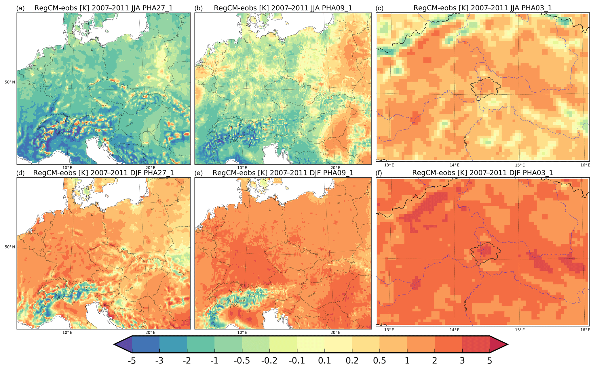
Figure 1 The difference between RegCM model near-surface temperature and E-OBS data for 2007–2011 JJA (a, b, c) and DJF (d, e, f) for the 27, 9 and 3 km domains (columns) in ^∘C. Note that the 27 km domain is cropped to show only the part corresponding to the 9 km domain. For the right panels, the administrative boundary of Prague is indicated too.

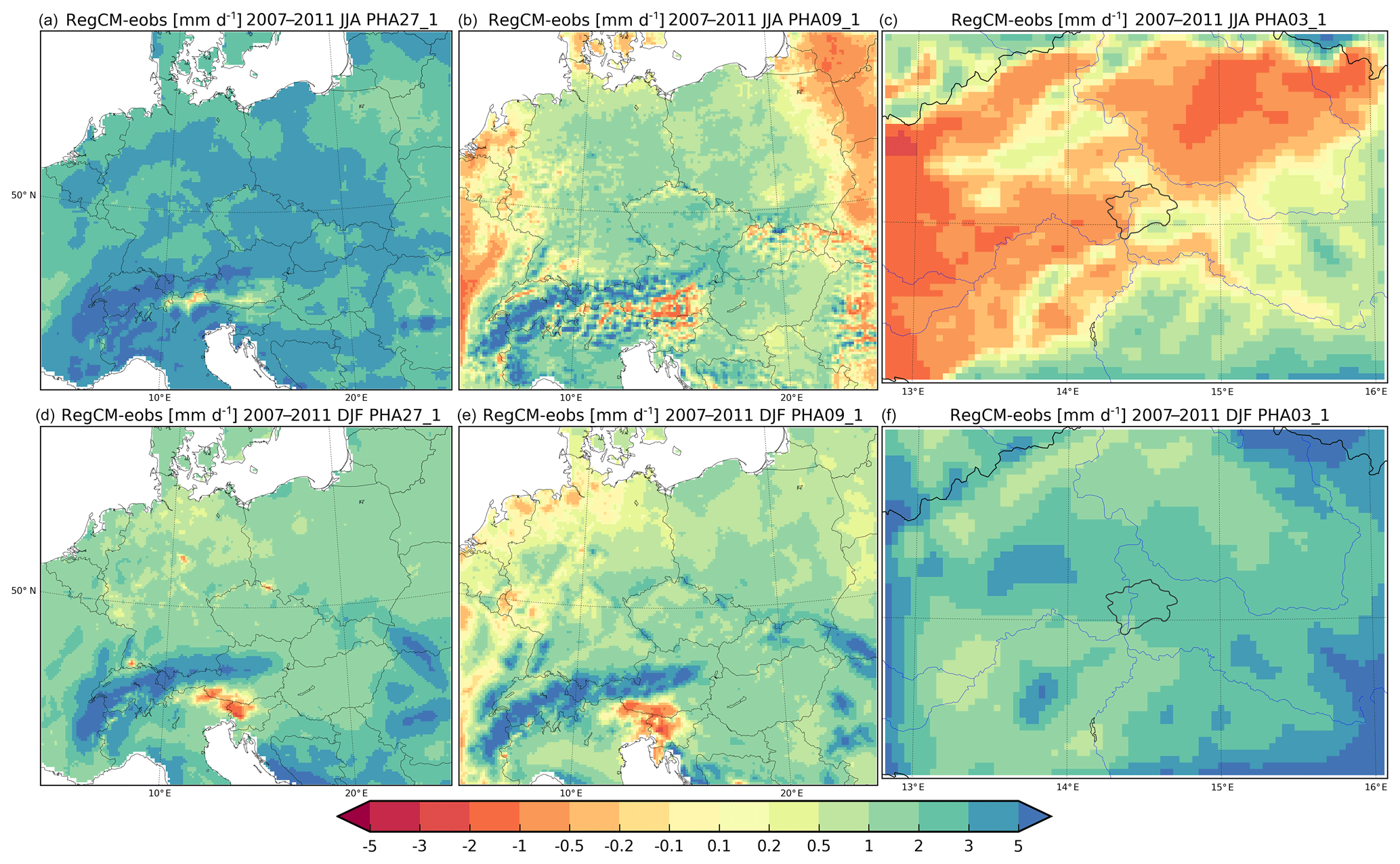
Figure 2 The difference between RegCM model precipitation and E-OBS data for 2007–2011 JJA (a, b, c) and DJF (d, e, f) for the 27, 9 and 3 km domains (columns) in mm d⁻¹. Note that the 27 km domain is cropped to show only the part corresponding to the 9 km domain. For the right panels, the administrative boundary of Prague is indicated too.

Since it is an offline coupled model, first, the RegCM model experiments were carried out. Afterwards, the meteorology-dependent BVOC emissions were computed by MEGAN. For each grid box, the fractional cover of different plant functional types and their emission factors determine the actual BVOC emission flux (i.e., for urban grid boxes it can be even zero). In the following, the meteorological inputs for CAMx are generated. Finally, BVOC emissions are combined with the anthropogenic emissions calculated by FUME. Having all inputs prepared, a series of CAMx simulations for the 2007–2011 period was conducted for each model domain, and these are summarized in Table 1. For RegCM, a pair of model experiments were performed, denoted “URBAN” and “NOURBAN”, where urban land surface was considered (and modeled with the CLMU model within RegCM) or replaced by rural surface most typical for the surroundings of the particular city (i.e., crops predominantly). The urban effects were thus calculated using the “annihilation method” (Baklanov et al., 2016), which has been often employed for urban studies but also for transport-related impact assessment (Huszar et al., 2013, e.g.,).

Table 1 Model simulations performed with RegCM (column 1) and CAMx (other columns). The second column denotes which urban effect is considered: NOURBAN – none; URB_t+q+uv – effect of temperature, humidity, wind; URB_t+q+uv+kv – effect of temperature, humidity, wind and turbulence. The third column lists the K_v methods used.

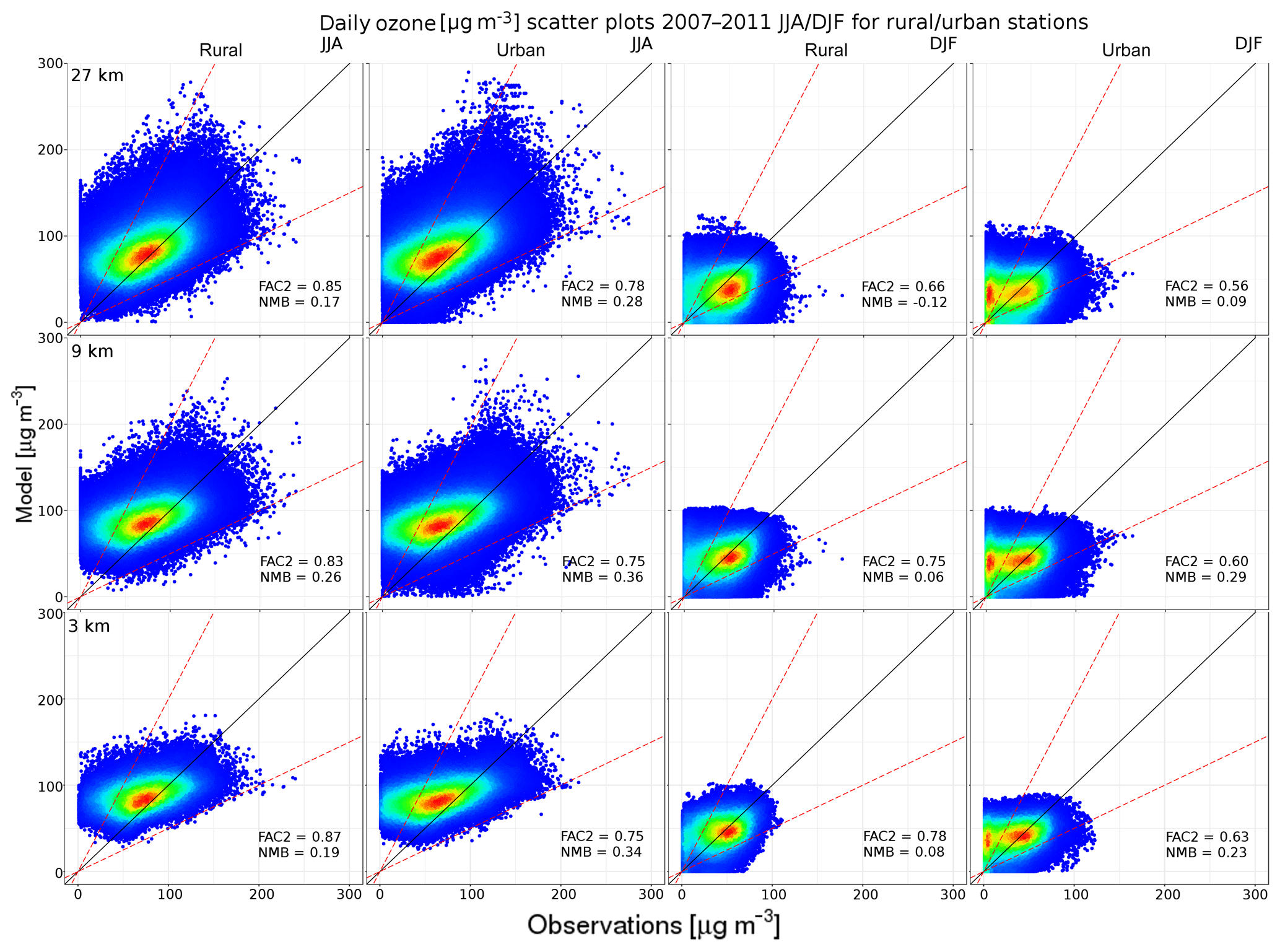
Figure 3 Scatter plots of daily ozone values for JJA (columns 1 and 2) and DJF (columns 3 and 4) for rural and urban stations in µg m⁻³. The rows represent different model resolutions from 27 km (top) to 3 km (bottom). Dot colors stand for the density of the model–observation pairs. Dashed red lines define the “factor-2” (FAC2) region. Calculated values of FAC2 and the normalized mean bias (NMB) are indicated too.

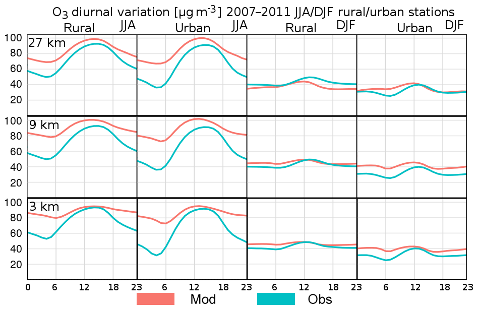
Figure 4 Comparison of average diurnal cycles of ozone with measurements µg m⁻³ for JJA (columns 1 and 2) and DJF (columns 3 and 4) for rural and urban background stations for the three domains (27, 9 and 3 km, from top to bottom): model (red) and observation (green).

Using RegCM meteorology, numerous of CAMx runs were carried out depending on which urban meteorological effects are considered and which K_v calculation method is employed. The “NOURBAN” reference CAMx run is driven by RegCM meteorology which does not consider any urban meteorological forcing, i.e., no temperature, humidity, wind and turbulence effects, which means it is driven by the NOURBAN RegCM runs. These CAMx experiments implement the CMAQ method for K_v calculation, which is the default option and was used also in Huszar et al. (2018a, b). Within the impact of the simulated meteorological changes on chemistry, the following effects were taken into account (1) modified temperature (t-impact); (2) modified absolute humidity (q-impact); (3) modified wind speed (uv-impact) and (4) modified vertical eddy diffusion coefficient; kv-impact). In a further set of simulations, denoted “URB_t+q+uv+kv”, all the listed effects were considered, and finally, in the “URB_t+q+uv” simulations, the kv-impact was removed. In addition, the “URB_t+q+uv+kv” and the “URB_t+q+uv” simulations were repeated with all listed K_v calculation methods. In this way, the total urban impact can be evaluated as the difference between the corresponding URB_t+q+uv+kv and NOURBAN model experiments. However, the main focus of the paper is the kv-impact (as URB_t+q+uv+kv minus URB_t+q+uv), which is now possible to evaluate by six different representations of vertical eddy diffusion. Each listed simulation is repeated for all model domains, which allows us to assess the sensitivity of results on horizontal model resolution too. In the case of the representation of meteorological conditions in AQ modeling, this can be relatively large (Tie et al., 2010). Finally, it has to be noted that for chemical simulations, the land use was kept the same for all model experiments in order to isolate the effect of meteorological changes on air quality.

3 Results

3.1 Model validation

Here, we provide a basic comparison of the most important modeled quantities to measured data (both the meteorology and air quality).

3.1.1 Meteorology

For meteorological variables, the gridded E-OBS van der Besselaar et al. (2011) data, which enable spatial comparison, were chosen to reflect the model values. The modeled average summer (JJA) and winter (DJF) near-surface temperatures and precipitation are evaluated for all model resolutions. Note that from the 27 km model domain, results are shown only over a subdomain corresponding roughly to the 9 km domain area to facilitate comparison. In Fig. 1, the difference between the modeled and measured near-surface temperatures is presented. During summer, the 27 and 9 km resolution simulations tend to underestimate surface temperatures by 2 ^∘C, while the 9 km one has smaller biases and even some overestimation occurs over the eastern part of the domain up to 1 ^∘C. Largest differences are encountered over mountainous areas, where the main reason lies probably in the poor model representation of complex orography. The 3 km simulation shows a warm bias almost everywhere up to 1–2 ^∘C (except a few areas near the Czech border). For the winter months, a warm model bias is seen at each resolution, being lowest in the 27 km one (up to 2 ^∘C) and reaches 3 ^∘C at 3 km resolution. Notably, the warm bias is largest over Prague (indicated by its borders), which suggests that the regional climate model used overestimates the urban temperature effects.

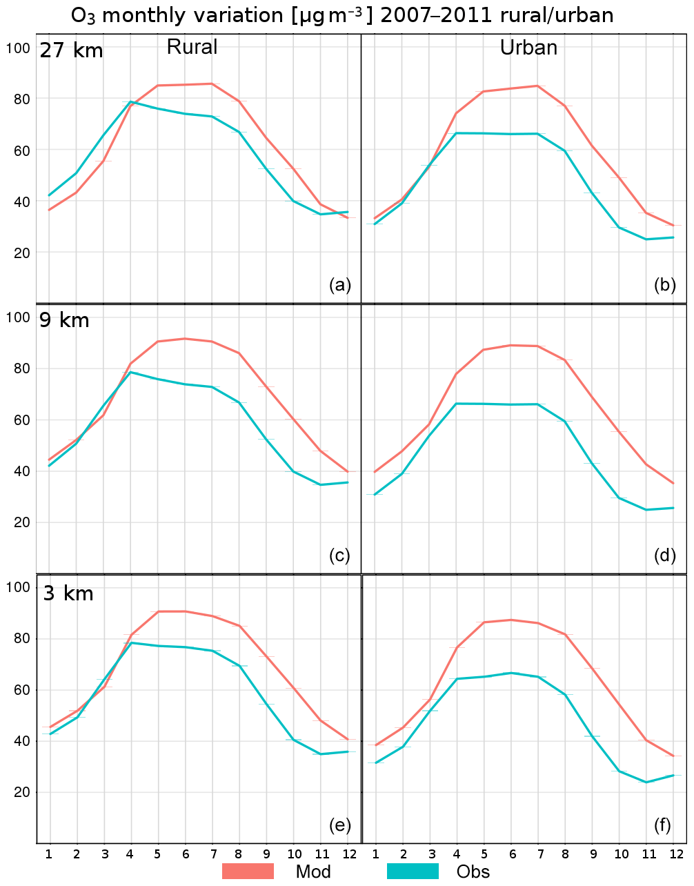
Figure 5 Comparison of monthly ozone values with measurements daily in µg m⁻³ for rural (a, c, e) and urban background stations (b, d, f) for the three domains (27, 9 and 3 km, from top to bottom): model (red) and observation (green).

The difference between the model total precipitation and observation is shown in Fig. 2 in mm d⁻¹. During winter, precipitation is overestimated in RegCM at each resolution, reaching up to 3–4 mm d⁻¹ above mountains. The medium-resolution model simulation shows somewhat smaller bias, while at 3 km and around Prague, the model overestimated rain by 2–3 mm d⁻¹. A different picture is seen during JJA: the low-resolution simulations show a strong overestimation of the precipitation by up to 2–3 mm d⁻¹ all over the domain. A much smaller positive model bias is encountered for 9 km, with values usually lower than 1 mm d⁻¹ (with even some negative bias over the domain edges). At the highest resolution, both positive and negative biases are present in the range of −3 to 2 mm d⁻¹. For the area of Prague, the bias is however small, lying between −0.5 to 0.5 mm d⁻¹.

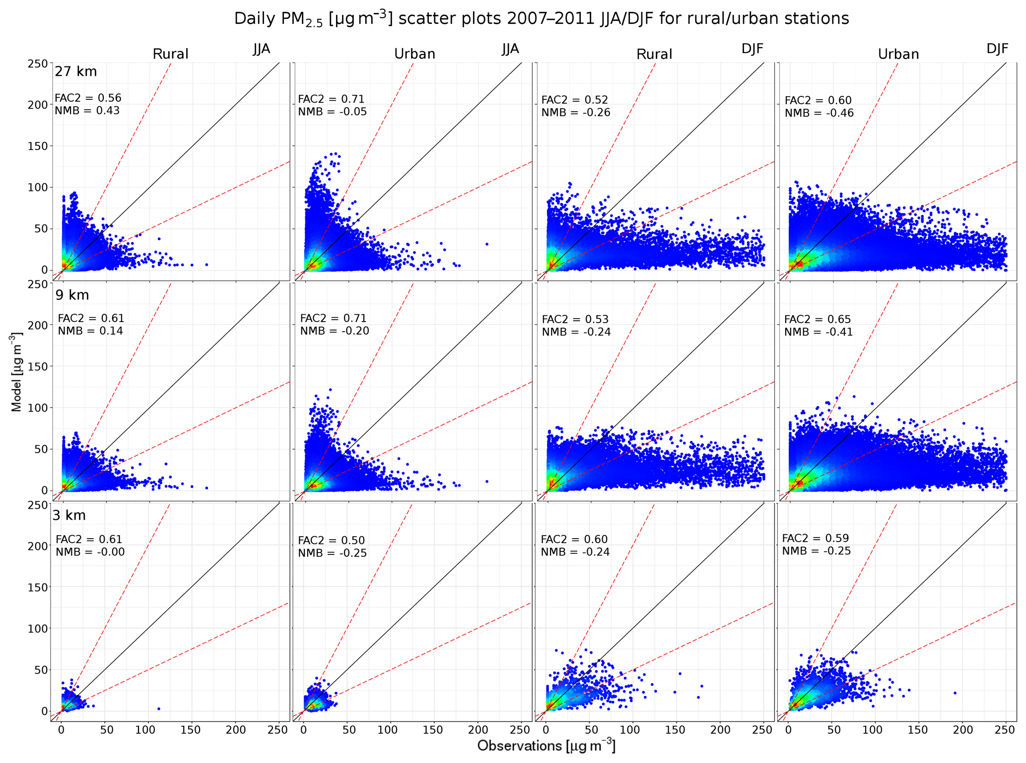
Figure 6 Scatter plots of daily PM_2.5 values for JJA (columns 1 and 2) and DJF (columns 3 and 4) for rural and urban stations in µg m⁻³. The rows represent different model resolutions from 27 km (top) to 3 km (bottom). Dot colors stand for the density of the model–observation pairs. Dashed red lines define the FAC2 region. Calculated values of FAC2 and the NMB are indicated too.

3.1.2 Air quality

The modeled surface concentrations were compared against the European Environment Agency AirBase (https://www.eea.europa.eu/data-and-maps/data/aqereporting-8, last access: 19 February 2020) station data. Rural and urban background stations were selected which are not affected by local sources unresolved by the models (i.e., traffic stations were not considered). The validation focuses on two key pollutants: O₃ and PM_2.5. Below, we use the term “modeled surface values” to mean the uniform concentration of the lowermost model layer at the corresponding grid box, which corresponds roughly to the urban canopy layer.

In Fig. 3, the scatter plots of measured and modeled ozone values are shown. It is seen that the vast majority of the values lie within a factor of 2 (i.e., conform to the FAC2). FAC2 is a robust measure, as it is weakly influenced by outliers (Chang and Hanna, 2004). FAC2 is lower in winter when observations exhibit very low values that are not resolved by the model, regardless of the relatively high resolution (3 km). In summer, model values are usually overestimated, and the overestimation is slightly higher at 27 and 9 km resolutions. It is also evident that the model provides a narrower range of values than measurements, especially during summer when it is unable to capture low ozone situations (large number of observation near zero, while model values are around 50 to 150 µg m⁻³).

The deviations seen in the scatter plots are better understood looking at the comparison of seasonal average diurnal cycles in Fig. 4. For summer, the average daily maximum ozone is reasonably captured with a little positive bias around 3–5 µg m⁻³ at 27 and 9 km resolutions, while urban stations have this bias slightly larger. The daily maximum ozone values are almost perfectly captured for 3 km resolution with a small overestimation for urban stations. The timing of the maxima is reasonably captured too. However, the model tends to strongly overestimate nighttime values for all resolutions and especially for urban stations. This explains the overall overestimation of average daily values seen in the scatter plots. For winter, model biases are smaller. For rural stations, the model underestimates measured values for the 27 km resolution and slightly overestimates for the higher ones. Here, however, the daily ozone maxima are well modeled. The observed urban values are overestimated by the model, especially during morning hours by up to 10 µg m⁻³; however, again, daily maxima are reasonably captured. The comparison of monthly means in Fig. 5 confirms the overestimation of ozone values during JJA (by 10–20 µg m⁻³), where the main contributors are the too-high ozone values during the night, as seen from the previous figure. On the other hand, winter (and spring) averages are modeled with higher accuracy, and even some underestimation by model occurs for the 27 km resolution (seen also in the diurnal cycles). Again, the positive model bias is somewhat larger for urban stations than background ones.

The daily PM_2.5 scatter plots in Fig. 6 and the corresponding normalized mean bias (NMB) values suggest that PM_2.5 is underestimated in the model, except for summer over rural stations at 27 km resolution. On the other hand, very good agreement in terms of this metrics is achieved for the 3 km resolution during JJA. It is seen that the underestimation is caused mostly by the high end of the observed values which CAMx is not able to reproduce. The FAC2 statistic is about 0.6–0.7 at each resolution and season. The gain in using higher resolution is not clear and the model improvement depends on which metric is analyzed. For rural stations, however, the 3 km simulations seem to be more accurate than the lower-resolution ones.

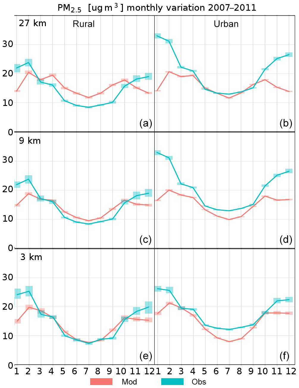
Figure 7 Comparison of monthly PM_2.5 concentrations with measurements daily in µg m⁻³ for rural (a, c, e) and urban background stations (b, d, f) for the three domains (27, 9 and 3 km, from top to bottom): model (red) and observation (green).

The monthly values in Fig. 7 bring some light to the root of model biases seen in scatter plots. Winter concentrations are underestimated by the model in each case by about 5–10 µg m⁻³ over rural stations and 10–15 µg m⁻³ over urban ones. During JJA and for rural stations, model concentrations of PM_2.5 tend to be higher than the measured ones by about 3–4 µg m⁻³ for the 27 km resolution, somewhat smaller for the 9 km one (about 2 µg m⁻³) and are in very good agreement for the fine-resolution simulations. Over urban stations, the model is consistently lower in PM_2.5 concentrations; here, however, the highest underestimation for JJA occurs at 3 km resolution (around 3–5 µg m⁻³).

It has to be noted that many urban background stations selected in the analysis are taken from small urban areas and their emission is not resolved well by the model. Therefore, the average urban model concentrations are only slightly different from rural ones (higher values for PM_2.5 in urban areas and lower ones for O₃ due to titration effects).

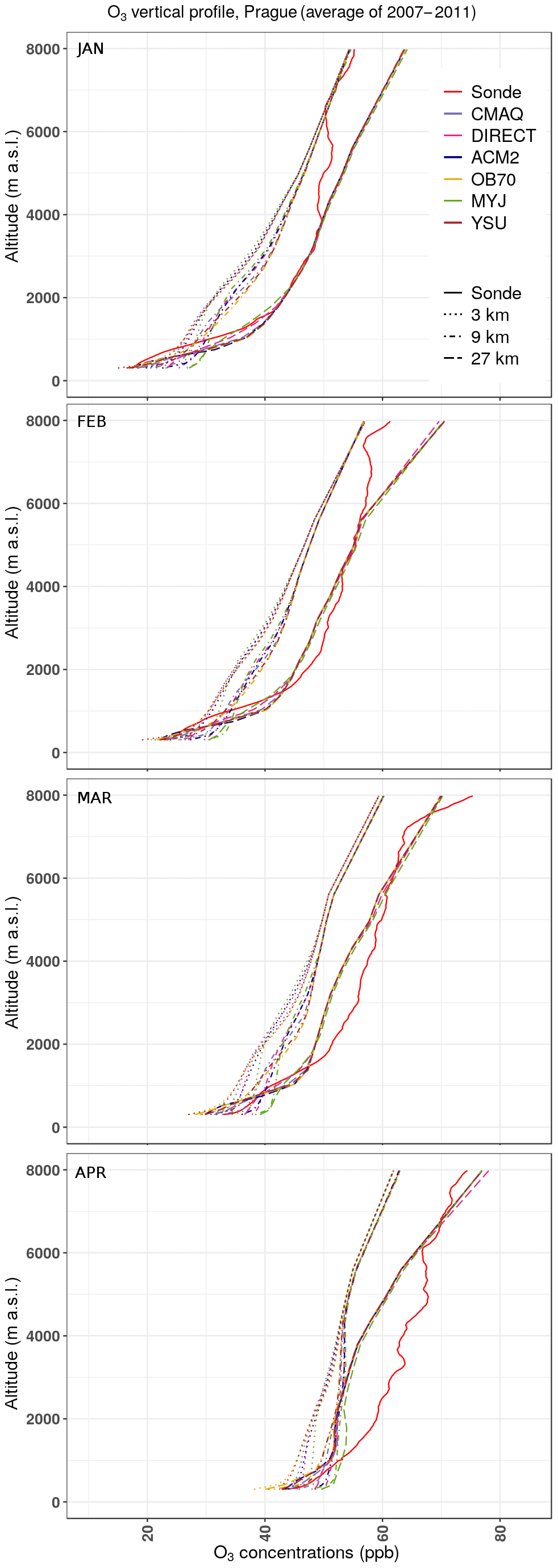
Figure 8 Comparison of monthly O₃ vertical profiles with sounding data for Prague, Czech Republic, for January–April. Solid red lines denote the measured data. Dashed, dot-dashed and dotted lines indicate the 27, 9 and 3 km resolution model data, and different colors indicate different K_v methods. Measurements are from 12:00 UTC each day. Concentrations are in ppbv. The vertical axis indicates the elevation above sea level.

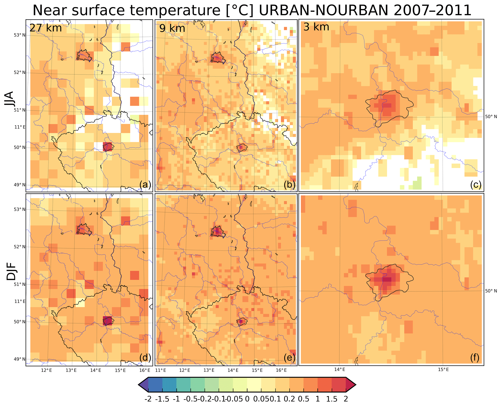
Figure 9 Impact of urban surfaces on near-surface temperature in ^∘C for JJA (a, b, c) and DJF (d, e, f) for the three resolutions (27, 9 and 3 km). Shaded areas represent statistically significant changes over the 98 % threshold using a two-tailed t test. The geographic locations of Berlin and Prague are indicated by their administrative boundaries.

Finally, to validate the model's ability to resolve the vertical transport and the sensitivity to the choice of K_v method, we contrasted the modeled pollutant profiles with available ozone sounding data for Prague, Czech Republic, measured for January to April at 12:00 UTC (see http://portal.chmi.cz/files/portal/docs/meteo/oa/sondaz_ozon.html, last access: 19 February 2020). Figure 8 shows a systematic underestimation of observed O₃ values occurring for elevations (above sea level) higher than about 1000 m, reaching 10 ppbv or even exceeding it. It is also clear that the coarse-resolution experiment tends to agree with the sounding data best, at least for the two winter months. On the other hand, the lowest ozone values are systematically modeled at the highest model resolution (3 km). Near the surface, ozone is usually overestimated by different simulations, while the 3 km resolution shows the best match. From the shape of the modeled profiles, it is also clear that the TKE-based MYJ method results in the most straight curve (highest values near the surface, lowest at high elevations) meaning that it produces the strongest mixing for ozone (see further in Sec. 3.2.3). On the other hand, the OB70 and YSU methods result in the most skewed ozone profiles at lower elevations (up to 1000 m) with the best agreement with observed values. In summary, it is difficult to conclude which resolution or K_v methods result in the best model–observation agreement. It seems that for higher elevations, coarse resolutions are more accurate, while at lower ones, the high-resolution simulations match observations better. Further, within the PBL, K_v methods producing lower K_v values (YSU and OB70) lead to ozone vertical patterns which most resemble the observations.

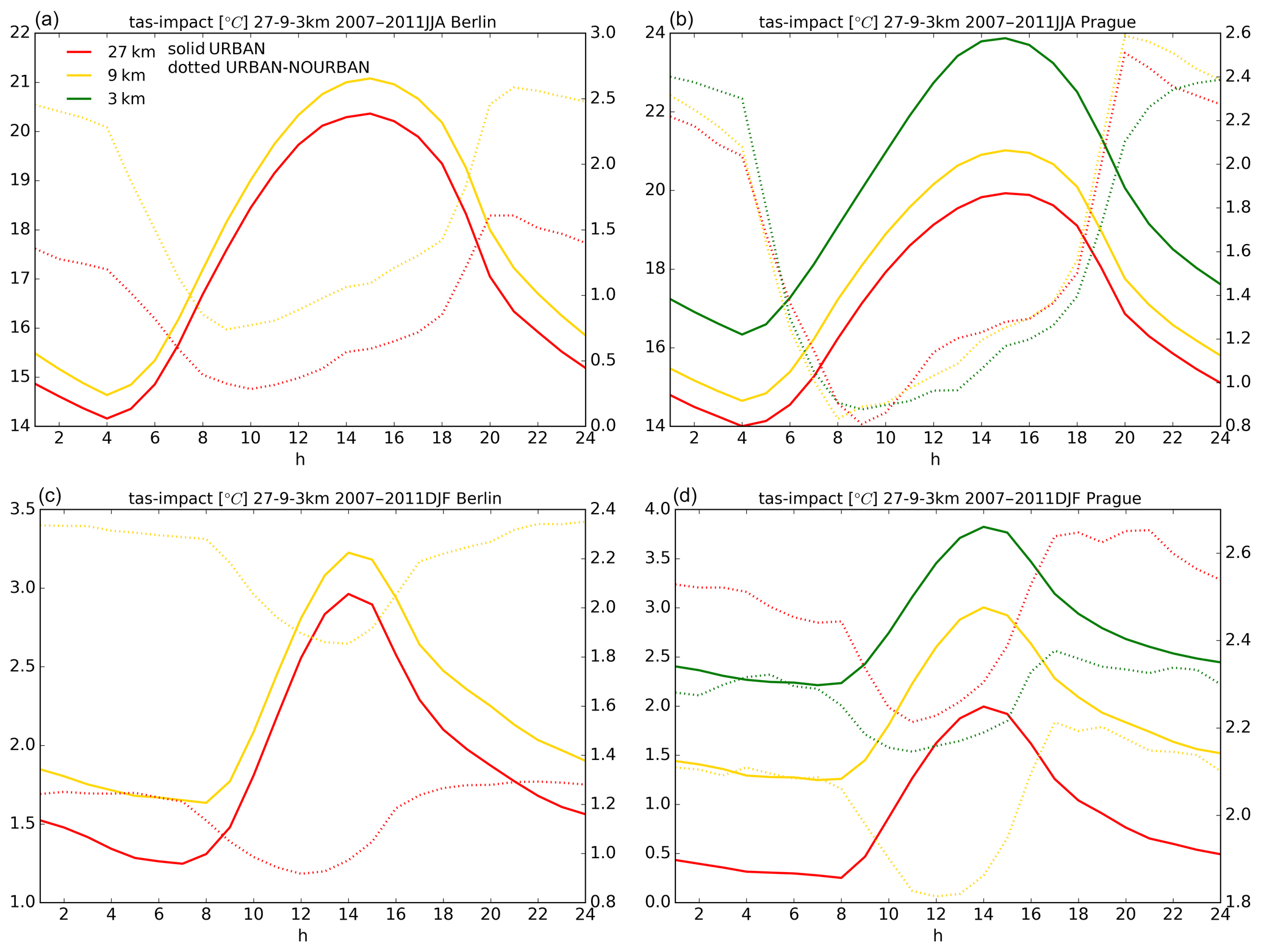
Figure 10 Impact of urban surfaces on near-surface temperature diurnal cycle in ^∘C for JJA (a, b) and DJF (c, d) for the three resolutions (27 km – red, 9 km – orange and 3 km – dark green). Solid lines are the absolute values (left-hand y axis) from the URBAN model experiment; dashed lines represent the urban impact (right-hand y axis).

3.2 Impact on meteorology

In our recent papers (Huszar et al., 2018a, b), we showed that urban canopies largely influence the local and regional summer values of temperature, humidity, wind speed and the vertical eddy diffusion coefficient (which determines the vertical turbulent transport). Here, we extend our analysis to winter months as well as to the sensitivity on the chosen horizontal grid resolution. It is widely known that, during winter months at stable stratification, buoyant turbulence is suppressed and the mechanical one dominates. Our analysis extended for winter thus brings new insight on how the urban canopy meteorological forcing acts on air quality under substantially different weather conditions compared to the hot season. Further, an important parameter to mesoscale modeling of urban meteorological effects is the model resolution which determines how well the urban land use heterogeneity is represented along with the (meso-)synoptic weather features that strongly influence the urban canopy meteorological phenomenon (e.g., UHI; Žák et al., 2019). The urbanization-induced meteorological effects (i.e., the UCMF) will be evaluated as the difference between RegCM URBAN and NOURBAN experiments. In spatial figures, results will be shown for the central European region that covers the two large cities we focus on (Berlin and Prague). These two cities will be the focus in the diurnal cycle figures too (except for results on the 3 km resolution, which covers only Prague).

3.2.1 Temperature

In Fig. 9, the spatial impact of urban canopy on near-surface temperature is shown. In general, the DJF impact on temperature is higher for both cities and exceeds 2 ^∘C. In summer, the impact lies between 1.5 and 2 ^∘C. Over Berlin, the 9 km simulation results in a more pronounced impact in both seasons. Over Prague, the impact is highest for the 27 km simulation in both seasons. It is also seen that if spatially averaged over coarse resolution, the high-resolution impact over Prague will be lower than over the 9 km and, especially, over the 27 km simulation. Further, the figure shows that most of the area analyzed exhibits statistically significant temperature impact, suggesting that even minor urbanized areas (small cities, villages) play a role in modulating near-surface temperatures.

The diurnal cycle of the urban canopy absolute temperatures and the difference compared to the non-urban case is shown in Fig. 10. It is seen that higher resolutions exhibit warmer urban canopy temperatures in accordance with the conclusions made in the validation. According to the expectations, maximum urban warming occurs during the evening at around 20:00–22:00 UTC (22:00 to 24:00 LT) for JJA. For DJF, the maximum difference occurs at different times over each city: for Berlin, it is around 00:00 UTC (01:00 LT); however, over Prague, it occurs earlier, around 04:00 to 08:00 UTC (05:00 to 09:00 LT). Over Berlin, the 9 km simulation results in almost 2 times higher impact (1 ^∘C vs. 2 ^∘C). Over Prague, the situation differs: the highest impact, in contrast to the absolute values, occurs for the 27 km simulation for DJF; however, for JJA, the results for the three resolutions are very close to each other and show maximum warming around 2.4 ^∘C.

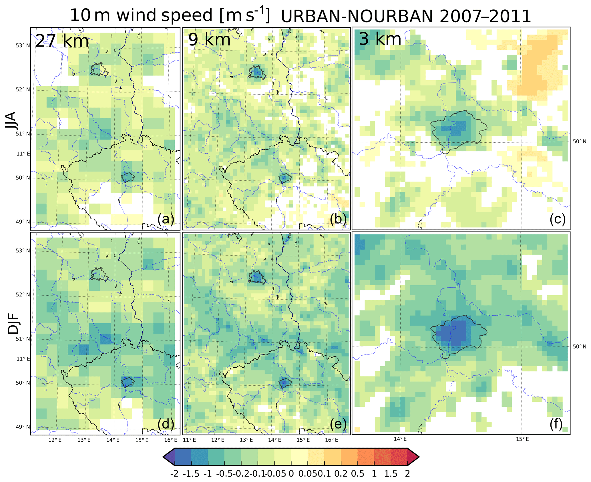
Figure 11 Impact of urban surfaces on 10 m wind speed in m s⁻¹ for JJA (a, b, c) and DJF (d, e, f) for the three resolutions (27, 9 and 3 km). Shaded areas represent statistically significant changes over the 98 % threshold using a two-tailed t test. The geographic locations of Berlin and Prague are indicated by their administrative boundaries.

3.2.2 Wind speed

In Fig. 11, the JJA and DJF average impact on 10 m wind speed is shown for the three resolutions. It is seen that the wind is significantly decreased over urbanized areas, while the decrease is higher in DJF (around −1.5 to −2 ms⁻¹ compared to −1 ms⁻¹). The smallest decrease is modeled for the 27 km simulation for both cities and seasons. Statistically significant changes on the 98 % level are modeled over a large part of the analyzed region, suggesting that even small urban areas contribute to the wind reduction significantly.

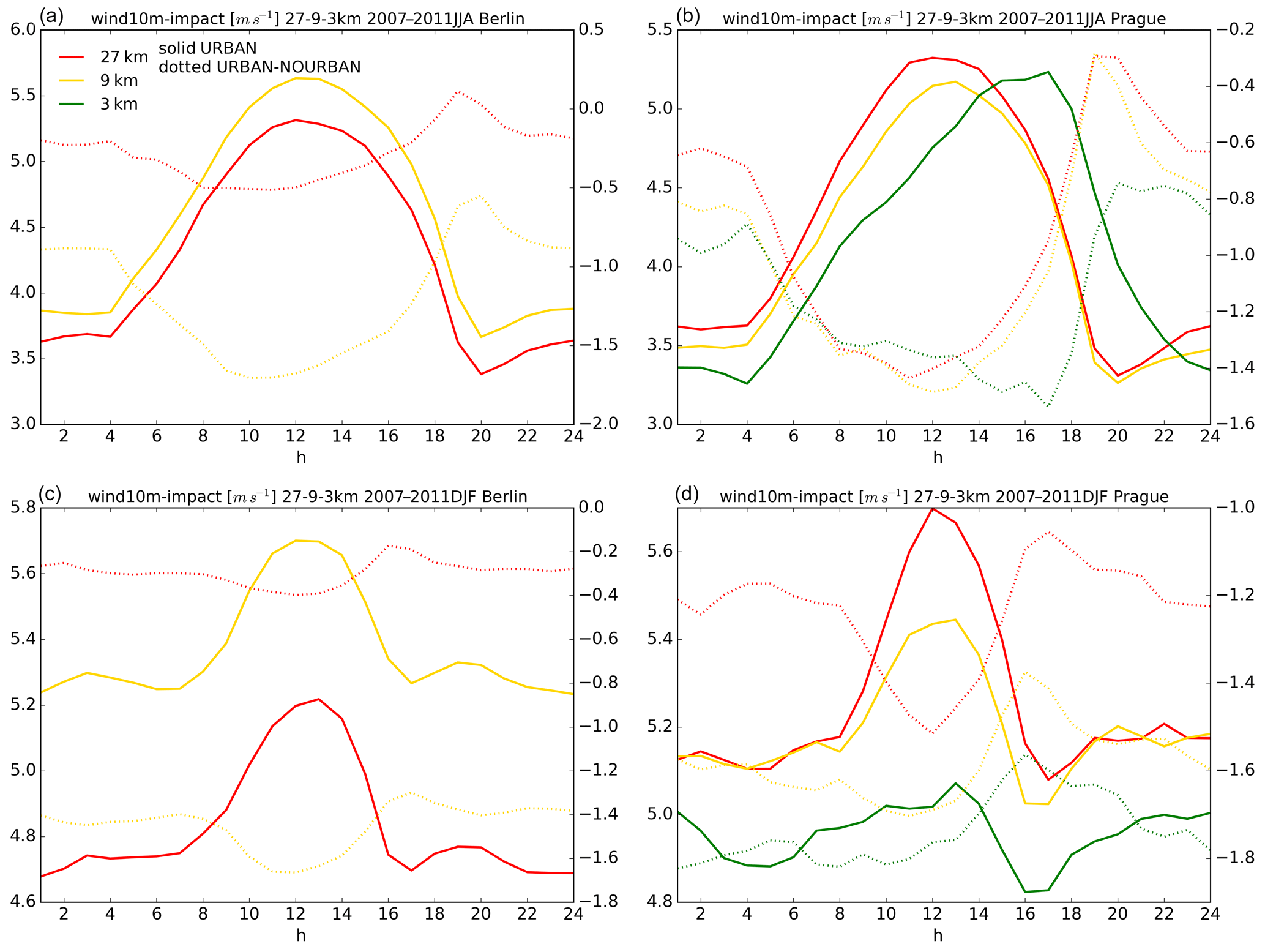
Figure 12 Impact of urban surfaces on the diurnal cycle of the 10 m wind speed in ms⁻¹ for JJA (a, b) and DJF (c, d) for the three resolutions (27 km – red, 9 km – orange and 3 km – dark green). Solid lines are the absolute values (left-hand y axis) from the URBAN model experiment; dashed lines represent the urban impact (right-hand y axis).

Regarding the diurnal cycle of the wind speed and its urban-canopy-induced changes in Fig. 12, it is seen that the two analyzed cities behave somewhat differently; while, over Berlin, the 27 km simulation produces lower winds than the 9 km one, over Prague, the lowest wind speeds are modeled for the highest resolution. A more unique picture (in accordance with the spatial figures) is seen for the impact itself. The higher the model resolution, the stronger the impact on winds. For Berlin, it reaches −1.5 ms⁻¹ for both seasons at noon. For Prague, the wind impact reaches −1.4 ms⁻¹ for JJA and can be as strong as −1.8 ms⁻¹ for DJF.

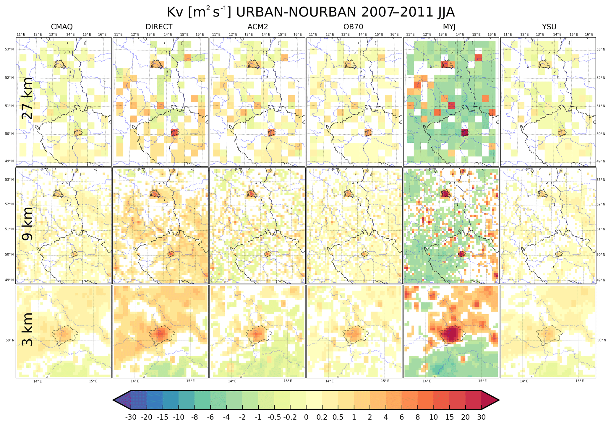
Figure 13 Impact of urban surfaces on the vertical eddy diffusion coefficient at 65 m in m² s⁻¹ for the 27 km (upper), 9 km (middle) and 3 km (lower row) for each K_v method (CMAQ, DIRECT, ACM2, OB70, MYJ and YSU, from left to right). Shaded areas represent statistically significant changes over the 98 % threshold using a two-tailed t test. The geographic locations of Berlin and Prague are indicated by their administrative boundaries.

3.2.3 Vertical eddy diffusivities

The main focus of this paper is the urban impact on the vertical eddy diffusion coefficient as a key factor determining urban pollution transport. Here, we present this impact for each of the K_v methods that are listed in Sect. 2.1.2. In Fig. 13, the urbanization-induced changes of the JJA eddy diffusion coefficient at the first model level (approximately 65 m, i.e., at urban canopy layer height) are shown for all three model resolutions (rows) and six K_v methods (columns). It is clear from each method/resolution that K_v values are affected the most over the two selected large cities (Berlin and Prague); however, statistically significant changes occur over rural areas too. The most striking feature is the wide range of K_v changes (predominantly increases). The smallest urbanization-induced increase is, in general, obtained for the CMAQ and YSU schemes: in both cases, the rural-to-urban transition results in about 1–2 m² s⁻¹ increase of K_v over both cities. The strongest increase is modeled with the TKE-based DIRECT and MYJ methods, where it reaches 15 and 30 m² s⁻¹, respectively. The ACM2 and OB70 methods lie in the middle range with increases up to 6–10 m² s⁻¹. Regarding the sensitivity of the resolution, its effect seems to be small, and the three resolutions result in a comparable change of K_v values, while often the 27 km resolution produces the strongest impact, especially when spatially averaging the higher-resolution results to 27 km. In summary, the urbanization-induced K_v changes above the urban canopy layer during JJA encompass a relatively wide range from 1 to 30 m² s⁻¹.

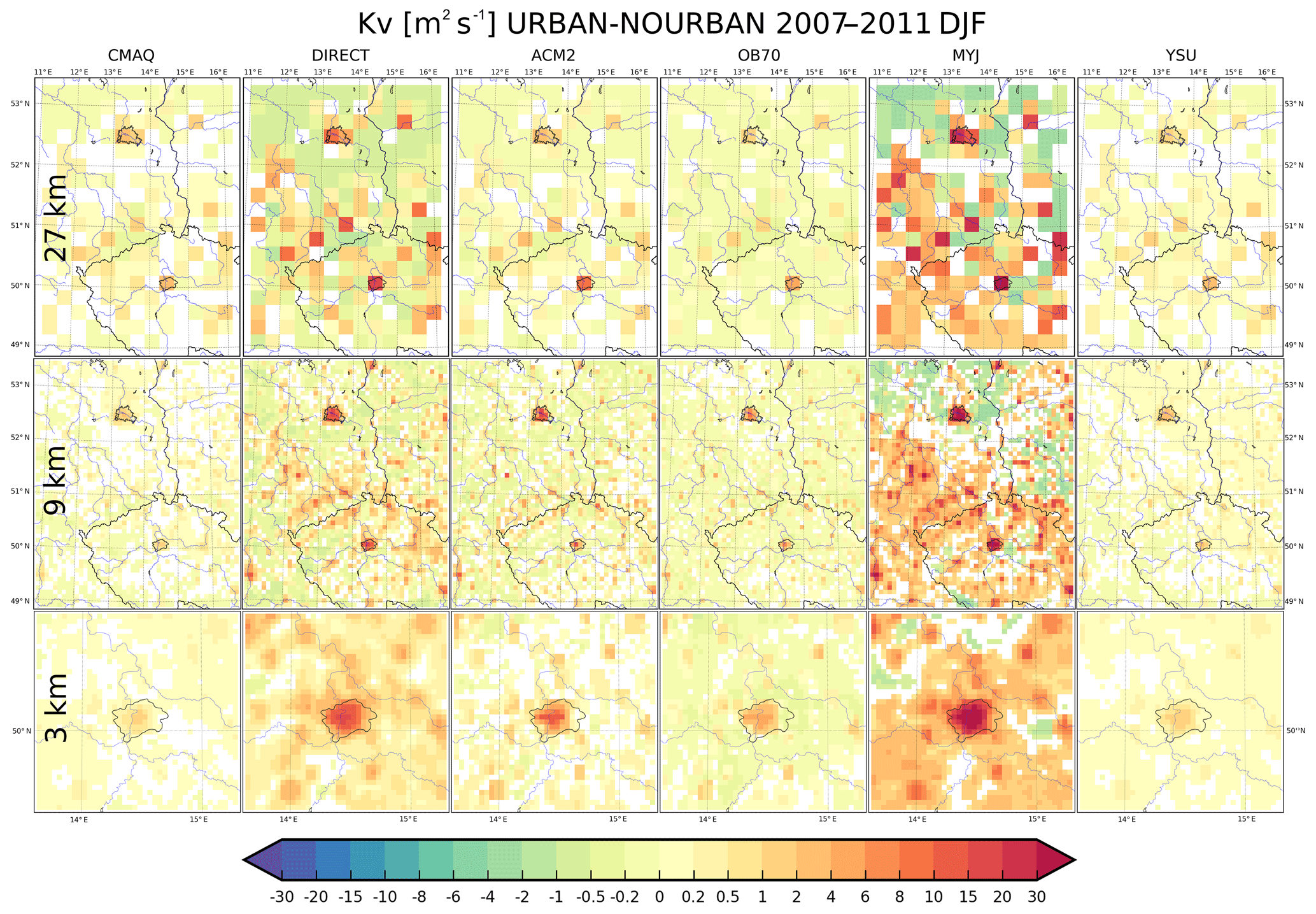
Figure 14 Same as Fig. 13 but for DJF.

The DJF impact on K_v at the canopy layer height is shown in Fig. 14, and very similar patterns are seen when compared to JJA, both qualitatively and quantitatively. The strongest impact is obtained for the two TKE-based methods (DIRECT and MYJ), reaching 15 to 30 m² s⁻¹. On the other hand, a 1 order of magnitude smaller impact is calculated for the CMAQ and YSU methods (up to 2 m² s⁻¹). Similarly to the JJA impact, the ACM2 and OB70 methods lie in the middle range of the K_v methods, with the former one somewhat stronger. During both seasons, a few areas encounter a statistically significant K_v decrease in the DIRECT and MYJ methods. This might be connected to the general wind reduction over large areas and the corresponding reduced TKE generation resulting in lower K_v values, but this would require more analysis.

Figure 15 Impact of urban surfaces on the diurnal cycle of the vertical eddy diffusion profile in m² s⁻¹ over Berlin for the 27 km (columns 1 and 3) and 9 km (columns 2 and 4) domains for both seasons (columns 1–2 for JJA, columns 3–4 for DJF). Individual rows represent different K_v methods (CMAQ, DIRECT, ACM2, OB70, MYJ and YSU, from top to bottom). Contour lines denote the absolute K_v values from the URBAN model experiment.

In order to understand the K_v evolution during the day, we plotted its diurnal cycle in Fig. 15 for Berlin. We are interested here not only in the urban canopy values but also in the impact on the whole K_v profile (within the PBL), and the absolute values from the URBAN model experiments are plotted as well as contour lines. Regarding the absolute values, it is seen that the largest K_v values are generated during early afternoon hours, in line with the expectations. The level of maximum K_v is higher in JJA (about 150–600 m) than during DJF (100–500) and also higher for the 9 km simulation compared to 27 km one. The TKE-based methods (DIRECT and MYJ) produce higher values, reaching 200 m² s⁻¹ for the DIRECT method and 120 m² s⁻¹ for MYJ in JJA. The lowest K_v values are calculated using the OB70 and YSU, reaching about 20 m² s⁻¹ in JJA. Winter K_v values are much lower, as expected. It is also seen that K_v values are usually larger for the 9 km simulation in both seasons. Here, the MYJ and DIRECT methods are the exceptions, with sightly higher values for the 27 km resolution. Somewhat distinct diurnal distribution is obtained with the ACM2 method. K_v values remain relatively large throughout the whole day, and the maximum value is reached at much higher levels than for other methods (around 500–800 m). Turning our attention to the urban-canopy-induced K_v changes (shaded colors), it is seen, again, that the highest impact is obtained using the DIRECT and MYJ methods, reaching 100 m² s⁻¹. It is also clear that the impact is higher during JJA and stronger for the 9 km resolution for all methods. The highest impact occurs at comparable levels to the absolute values and consistently around late afternoon to early evening hours for each method. This means that the maximum of the impact is shifted to 3 to 6 h later than the occurrence of the maximum absolute values. The smallest impact is simulated for the YSU and OB70 methods, reaching 10–20 m² s⁻¹ at their maximum, which occurs in afternoon/early evening hours.

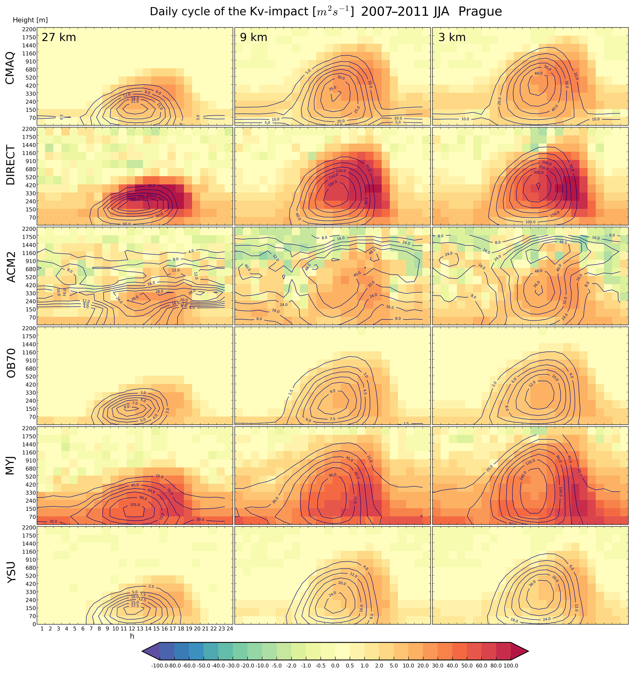
Figure 16 Impact of urban surfaces on the JJA diurnal cycle of the vertical eddy diffusion profile in m² s⁻¹ over Prague for the 27, 9 and 3 km domains (columns from left to right). Individual rows represent different K_v methods (CMAQ, DIRECT, ACM2, OB70, MYJ and YSU, from top to bottom). Contour lines denote the absolute K_v values from the URBAN model experiment.

In Fig. 16, the absolute K_v values and the urban canopy impact are shown for Prague for JJA in the same manner as for Berlin, only extended by the 3 km simulation. In general, both the absolute K_v values as well as the impact is very similar to the impact over Berlin. The absolute eddy diffusion coefficient increases with increasing resolution and is, again, highest for the DIRECT and MYJ methods reaching 350 and 150 m² s⁻¹, respectively. The lowest K_v values are obtained when calculated by the YSU and OB70 methods (up to 20 m² s⁻¹). It is also clear that, at higher resolutions, the maximum K_v occurs at higher model levels. Regarding the impact, there is a very clear increase when going into higher resolutions, and the change is especially large between the 27 and 9 km resolutions.

Figure 17 Impact of urban surfaces on the DJF diurnal cycle of the vertical eddy diffusion profile in m² s⁻¹ over Prague for the 27, 9 and 3 km domains (columns from left to right). Individual rows represent different K_v methods (CMAQ, DIRECT, ACM2, OB70, MYJ and YSU, from top to bottom). Contour lines denote the absolute K_v values from the URBAN model experiment.

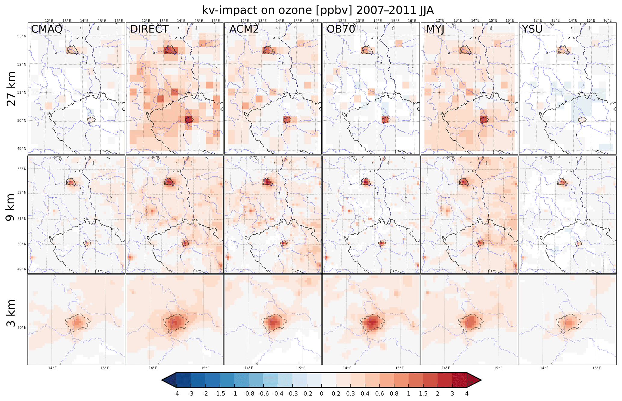
Figure 18 The impact of urbanization-induced K_v enhancement (i.e., increase of vertical eddy diffusivity) on surface O₃ concentrations in ppbv for the 27, 9 and 3 km resolutions (top to bottom) for JJA for the six K_v methods (CMAQ, DIRECT, ACM2, OB70, MYJ and YSU). The geographic locations of Berlin and Prague are indicated by their administrative boundaries. Shaded areas represent statistically significant changes on the 98 % level using a two-tailed t test.

During DJF (Fig. 17), absolute K_v values are, of course, smaller compared to summer ones; however, one cannot clearly conclude an increase when turning to higher resolutions. For example, for the DIRECT and MYJ methods, the 27 km results are higher than those obtained for the 9 and 3 km simulations. However, these two methods still produce the largest vertical diffusivities (up to 40–50 m² s⁻¹, with MYJ being higher). Regarding the urban canopy impact, the DIRECT and MYJ methods result in the strongest change. However, in contrast to Berlin (or to the Prague JJA results), the strongest impact is modeled at 27 km resolution, while for other K_v methods, the difference between individual resolution is not significant.

3.3 Impact on the air quality

The chemical changes, in particular the changes in the concentrations of O₃ and PM_2.5 as a result of the simulated urban canopy meteorological forcing (seen above), are presented here. This includes the effects of modified temperature, wind and vertical diffusivity, which were analyzed in the previous section. The effect of the urban-canopy-induced modifications of humidity is included too. However, we showed in Huszar et al. (2018b) that the impact is negligible. In accordance with Huszar et al. (2018b), we will distinguish different impacts based upon which urban meteorological perturbation is considered: e.g., the “t+q+uv-impact” indicates the combined impact of temperature, humidity and wind changes; the “kv-impact” stands for the chemical changes triggered by modified vertical eddy diffusion values only; and the “t+q+uv+kv-impact” indicates the impact of all considered urban canopy meteorological changes which, in this paper, will be equivalent to the “total-impact”. We will start with the impact of enhanced turbulent transport which is the main focus of this paper.

3.3.1 The effect of perturbed diffusivities

In Figs. 13–17, we presented the range of K_v perturbation caused by the introduction of urban land surfaces, and it was seen that it covers 2 orders of magnitude (increases from a few m² s⁻¹ to tens of m² s⁻¹). Here, our attention moves to the range of perturbations of O₃ and PM_2.5 urban canopy concentrations this leads to (i.e., the kv-impact is evaluated for individual K_v methods).

Ozone

Figure 18 presents the JJA changes of O₃ due to the urbanization-induced K_v enhancement for the three resolutions and six K_v methods. Ozone is increased in all cases, ranging from 0.2 to 3 ppbv (about 5 %–10 %), as expected following Huszar et al. (2018a). They showed that the main contributor to this increase is the reduced destruction due to the turbulence-enhanced vertical removal of NO_x from the canopy layer and the increased turbulent flux from the RL during the night. The smallest increase is modeled by the CMAQ and YSU methods. At 27 km resolution, the largest effect is obtained using the DIRECT method; at 9 km, the four remaining methods give a rather comparable impact for both cities. At 3 km resolution, the largest impact is seen for the ACM2 and OB70 methods. For Berlin, higher resolution leads to a stronger impact for each method. For Prague, it is most often the 27 km resolution where the highest impact is modeled (expect YSU). In general, the impact over Berlin is stronger than that over Prague.

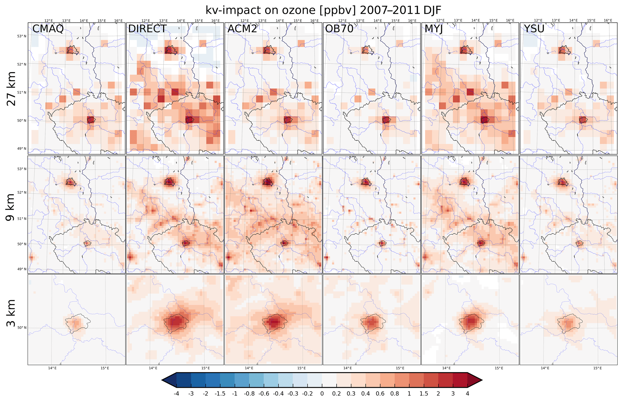
Figure 19 Same as Fig. 18 but for DJF.

The DJF impact in Fig. 19 is stronger than the JJA one, often reaching 4–5 ppbv (up to 30 %–40 % change). Here, again, the smallest effect is obtained using the CMAQ and YSU methods. The strongest one is seen for the DIRECT, MYJ and ACM2 methods at each resolution. It is also clear that higher resolution usually leads to smaller modeled impact.

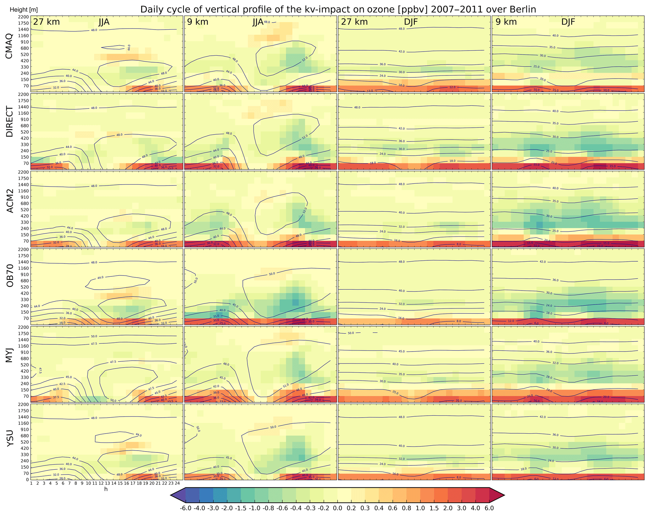
Figure 20 The impact of the urbanization-induced K_v enhancement (i.e., increase of vertical eddy diffusivity) on the diurnal cycle of the O₃ profile over Berlin for JJA (columns 1–2) and DJF (columns 3–4) evaluated over the 27 km (columns 1 and 3) and 9 km (columns 2 and 4) domains. Rows correspond to individual K_v methods. Colors indicate the difference; contours stand for the absolute concentrations (from the total-impact). Units are in ppbv.

To gain a more detailed insight into the range of kv-impacts, we also plotted the diurnal cycle of the vertical profile above both analyzed cities along with the absolute values. In Fig. 20, we present the results for Berlin for both seasons. Regarding the absolute values in JJA, at higher levels, they are higher and this elevated maximum (usually around 200–500 m) “reaches” the surface as the usual early afternoon summer ozone maxima occur (about 40–50 ppbv). These are somewhat higher at 9 km resolution. Turning our attention to the impact, a very clear maximum is seen near the surface during early evening, reaching 6 ppbv, while the effect is stronger for the 9 km resolution. This maximum is not visible only for the OB70 method at 27 km resolution. Another striking feature is the ozone decrease up to −2 ppbv at higher levels (200–400 m) with maximum intensity coinciding with the maximum surface increase and slightly shifted compared to maxima of the absolute values. In general, the impact (similarly to the absolute values) is more pronounced for the 9 km resolution and reaches higher levels. A secondary ozone maximum in the daily cycle is detectable from noon to the evening at altitudes around 500–1500 m (higher altitudes at 9 km resolution), reaching 0.3–0.4 ppbv. During DJF, the pattern of absolute values is much simpler, with gradually increasing concentrations with increasing altitude including the expected weak afternoon maximum. The 9 km resolution profiles usually have lower values compared to 27 km ones, except near the surface when the ACM2 method provides higher values. The kv-impact on O₃ is characterized by a clear increase at the surface model layer with a weak maximum during late afternoon up to 6 ppbv, while the strongest effect is modeled for the DIRECT and ACM2 methods. The diurnal amplitude of the impact is much smaller than during JJA and it is clearly stronger for the 9 km resolution than for the 27 km one. The O₃ decrease at higher levels is well seen (around 300–400 m; up to −2 ppbv reduction) and it is much stronger for the 9 km resolution.

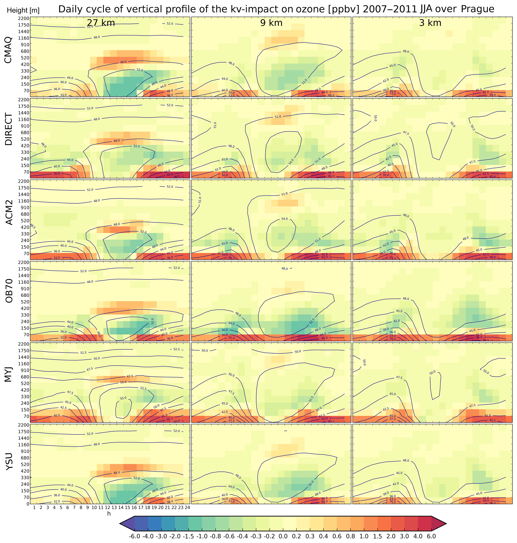
Figure 21 The impact of the urbanization-induced K_v enhancement (i.e., increase of vertical eddy diffusivity) on the diurnal cycle of the O₃ profile over Prague for JJA. Columns represent the three resolutions (27, 9 and 3 km, from left to right). Rows correspond to individual K_v methods. Colors indicate the difference; contours stand for the absolute concentrations (from the total-impact). Units are in ppbv.

The pattern of the kv-impact on O₃ as well as that of the absolute values is very similar for Prague compared to Berlin, as seen in Fig. 21. The O₃ increase is limited to the lowermost layers and there is again a clear early evening maximum reaching 5–6 ppbv. The impact reaches almost zero values during midday near the surface, as seen for Berlin too. The decrease at higher levels (200–400 m) with maximum during late afternoon/early evening is evident from model results too and reaches −2 to −4 ppbv. Finally, the secondary maximum of O₃ increase during noon hours at around 500–1500 m occurs as well and reaches 1 ppbv. The impact for the 3 km resolution seems to be the smallest, probably in connection with the fact that the absolute values are the smallest at this resolution.

Figure 22 Same as Fig. 21 but for DJF.

During DJF, over Prague (Fig. 22), both the absolute values and the kv-impact resemble the pattern seen for Berlin. The diurnal amplitude is much smaller for the impact, with maxima usually around early evening, and occasionally a weaker maximum is seen during morning hours for the DIRECT, ACM2, OB70 and MYJ methods. Again, the smallest impact is modeled for the CMAQ and YSU methods, and the values for the 3 km resolution are below those for lower resolutions. The ozone decrease at higher altitudes (around 200–500 m) is detectable too, reaching −2 ppbv.

In summary, different K_v methods lead to not only different average kv-impact on ozone values but substantially different vertical profiles and different shape of the daily cycle including the timing of the maximum value and occurrence of secondary maxima at higher altitudes.

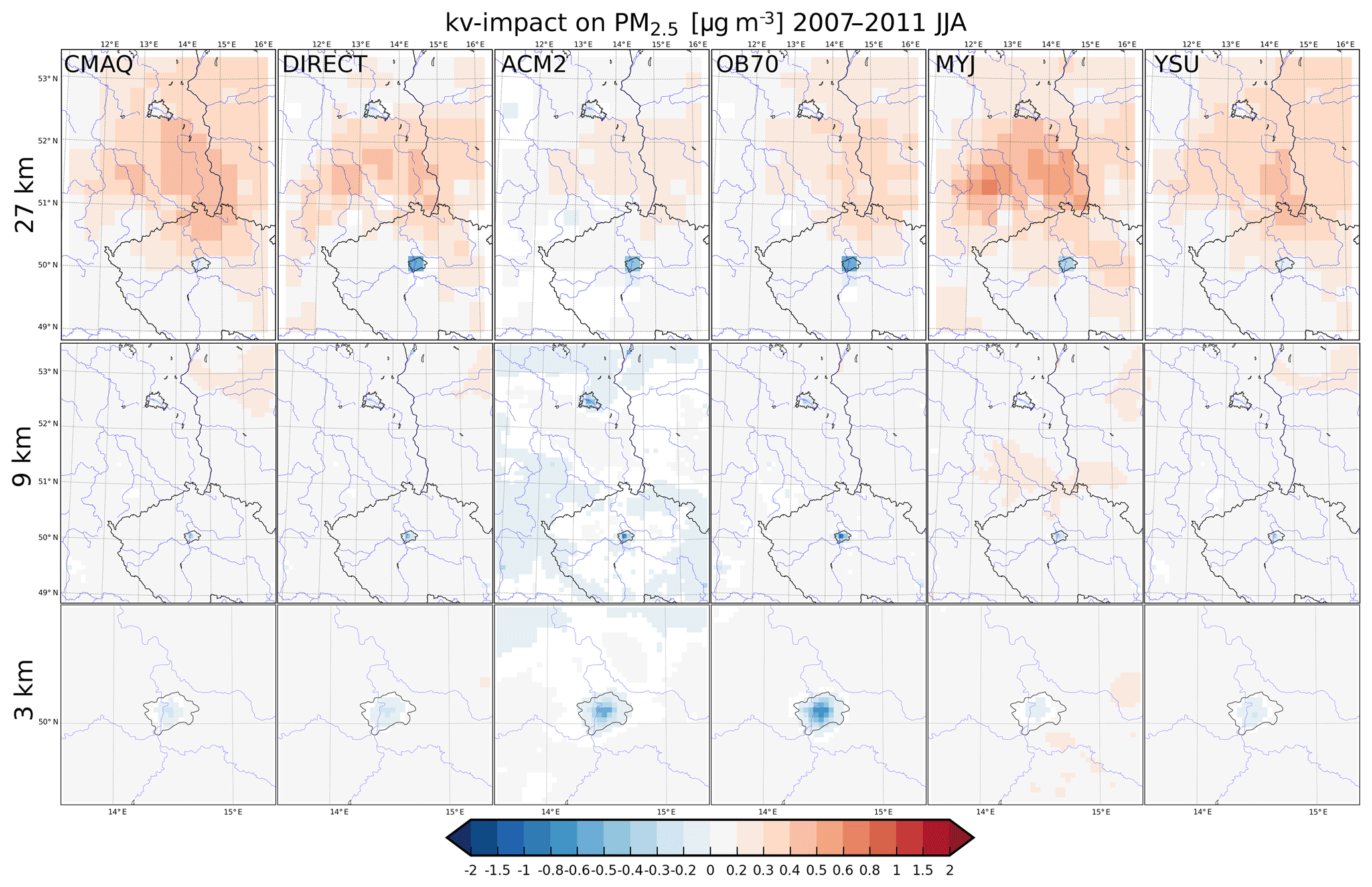
Figure 23 The impact of urbanization-induced K_v enhancement (i.e., increase of vertical eddy diffusivity) on surface PM_2.5 concentrations in µg m⁻³ for the 27, 9 and 3 km resolutions (top to bottom) for JJA for the six K_v methods (CMAQ, DIRECT, ACM2, OB70, MYJ and YSU). The geographic locations of Berlin and Prague are indicated by their administrative boundaries. Shaded areas represent statistically significant changes on the 98 % level using a two-tailed t test.

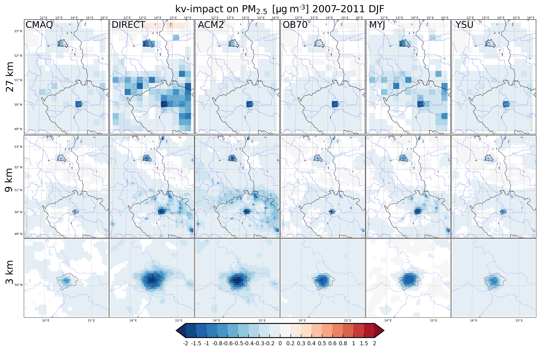
Figure 24 Same as Fig. 23 but for DJF.

PM_2.5

Our attention now turns to the UCMF-induced PM_2.5 changes, and we first look at the changes in near-surface concentrations due to the kv-impact. The results for JJA and DJF are presented in Figs. 23 and 24, respectively. For JJA and for Prague, there is a clear decrease of PM_2.5, in line with the expectation of higher vertical turbulent removal (dispersion) of aerosol as well as their precursors from the urban canopy layer (Huszar et al., 2018b). In general, the 27 km resolution leads to stronger decrease of up to −2 µg m⁻³, especially for the DIRECT, ACM2 and OB70 methods. For higher resolutions, these methods result in the largest impacts too (−1 to −2 µg m⁻³), while very weak impact is modeled using the CMAQ and YSU methods (from −0.2 to −0.4 µg m⁻³). A slightly different picture is obtained for the kv-impact for Berlin. While at 9 km resolution, the conclusions are very similar to the ones seen for Prague (decreases of PM_2.5 of similar magnitude; ACM2 and OB70 providing the strongest impact), at 27 km resolution, the impact is either a very small decrease (DIRECT and ACM2, up to −0.2 µg m⁻³) or a slight increase up to 0.3 µg m⁻³ for the remaining methods. It is seen that there is a general increase of PM_2.5 over a large part of the analyzed region and this increase dominates the impact over Berlin. This is probably caused by the PM_2.5 removed from the urban atmosphere (due to higher K_v values) and transported to and deposited in other regions, causing an opposite effect.

During DJF, the kv-impact leads to clear increase of PM_2.5 concentrations for all resolutions, cities and methods. The strongest impact is seen for the DIRECT, ACM2 and MYJ methods, peaking at −2 µg m⁻³, while, again, the smallest impact is obtained for the CMAQ and YSU methods (below −1 µg m⁻³). It is also clear that the impact calculated for lower resolutions is usually slightly stronger, especially over Prague.

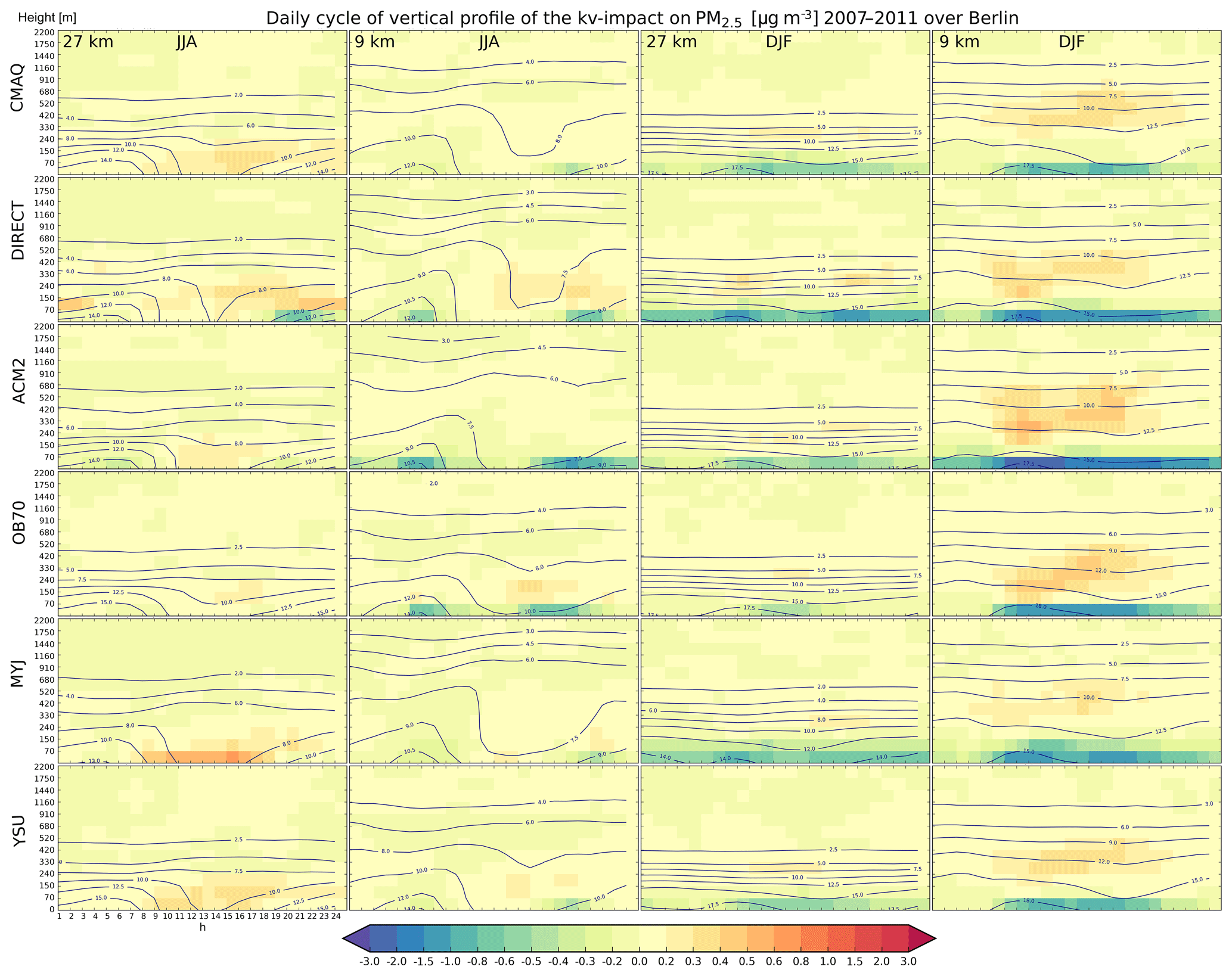
Figure 25 The impact of the urbanization-induced K_v enhancement (i.e., increase of vertical eddy diffusivity) on the diurnal cycle of the PM_2.5 profile over Berlin for JJA (columns 1–2) and DJF (columns 3–4) evaluated over the 27 km (columns 1 and 3) and 9 km (columns 2 and 4) domains. Rows correspond to individual K_v methods. Colors indicate the difference; contours stand for the absolute concentrations (from the total-impact). Units are in µg m⁻³.

In order to see how the kv-impact on PM_2.5 evolves during the day, we plotted in Fig. 25 the diurnal cycle of the impact of urbanization-induced K_v enhancement on the PM_2.5 vertical profiles along with the absolute values. At the surface, the absolute values are higher during DJF (18 µg m⁻³) compared to JJA (up to 15 µg m⁻³) as expected due to the more stagnant meteorological conditions. However, at higher elevations, JJA concentrations are higher due to enhanced vertical transport from the canopy layer. It is also clear that for the 9 km resolution, PM_2.5 decreases with height slower than in the 27 km run, which is in line with the slightly stronger vertical mixing in the 9 km resolution compared to 27 km one (see Fig. 15). Further, it is seen that the K_v methods giving stronger vertical turbulent diffusivities (e.g., DIRECT) result in lower near-surface concentrations, and vice versa (e.g., OB70), especially for JJA. The diurnal cycle of the absolute values is characterized by a clear maximum during morning hours and a minimum (especially in JJA) during afternoon. Looking at the kv-impact on PM_2.5 concentrations, it is seen that the near-surface values are characterized by decreases except the 27 km simulation values during JJA (in line with Fig. 23). At 9 km resolution, during JJA, this decrease encompasses two peaks: a primary peak during the afternoon reaching −1 µg m⁻³ and a secondary one during morning (up to −0.6 µg m⁻³). The strongest impact is provided by the DIRECT, ACM2 and OB70 methods, as seen in the spatial figure above. At higher altitudes, the PM_2.5 removed from the urban canopy layer causes a positive impact “region” (at about 100–300 m) up to 0.3–0.4 µg m⁻³ occurring during the afternoon. At 27 km resolution, however, this elevated maximum reaches the ground and leads to an almost complete disappearance of surface decreases. During DJF, the two resolutions behave qualitatively in a very similar way. Both lead to a well-pronounced surface PM_2.5 decrease, while it is stronger in the 9 km resolution (up to −2 to −3 µg m⁻³). The DIRECT and ACM2 methods provide the largest impact. The double-peak shape of the near-surface impact is less clear or missing; instead, the kv-impact remains high from morning to evening hours. The elevated increase of PM_2.5 is more pronounced during the cold season and is, similarly to JJA, stronger over at 9 km resolution, reaching 0.5–0.6 µg m⁻³ at about 200–500 m.

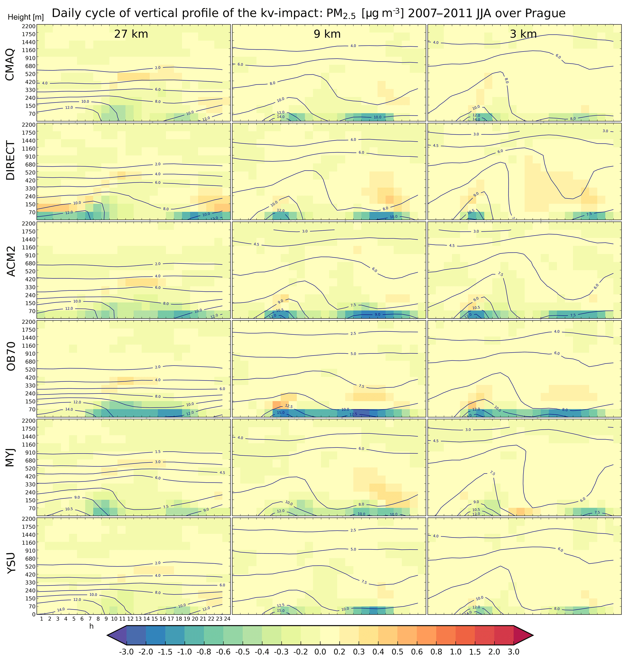
Figure 26 The impact of the urbanization-induced K_v enhancement (i.e., increase of vertical eddy diffusivity) on the diurnal cycle of the PM_2.5 profile over Prague for JJA. Columns represent the three resolutions (27, 9 and 3 km, from left to right). Rows correspond to individual K_v methods. Colors indicate the difference; contours stand for the absolute concentrations (from the total-impact). Units are in µg m⁻³.

For Prague, the JJA absolute values in Fig. 26 look quantitatively and qualitatively very similar to those over Berlin, with peak values around 10–15 µg m⁻³ during morning hours, while higher values are modeled with K_v methods producing lower K_v values (e.g., OB70). The kv-impact manifests again as two maxima of the near-surface PM_2.5 decrease, reaching −2 to −3 µg m⁻³. The strongest impact is seen for the DIRECT, ACM2 and OB70 methods, as is seen for Berlin too. The elevated positive impact seen for Berlin is present here too and reaches 0.5–0.6 µg m⁻³ with two maxima: one during morning hours and one during evening hours. In general, the impact over the 9 and 3 km resolutions (up to −3 µg m⁻³) is stronger than that over 27 km (up to −1.5 µg m⁻³).

Figure 27 Same as Fig. 26 but for DJF.

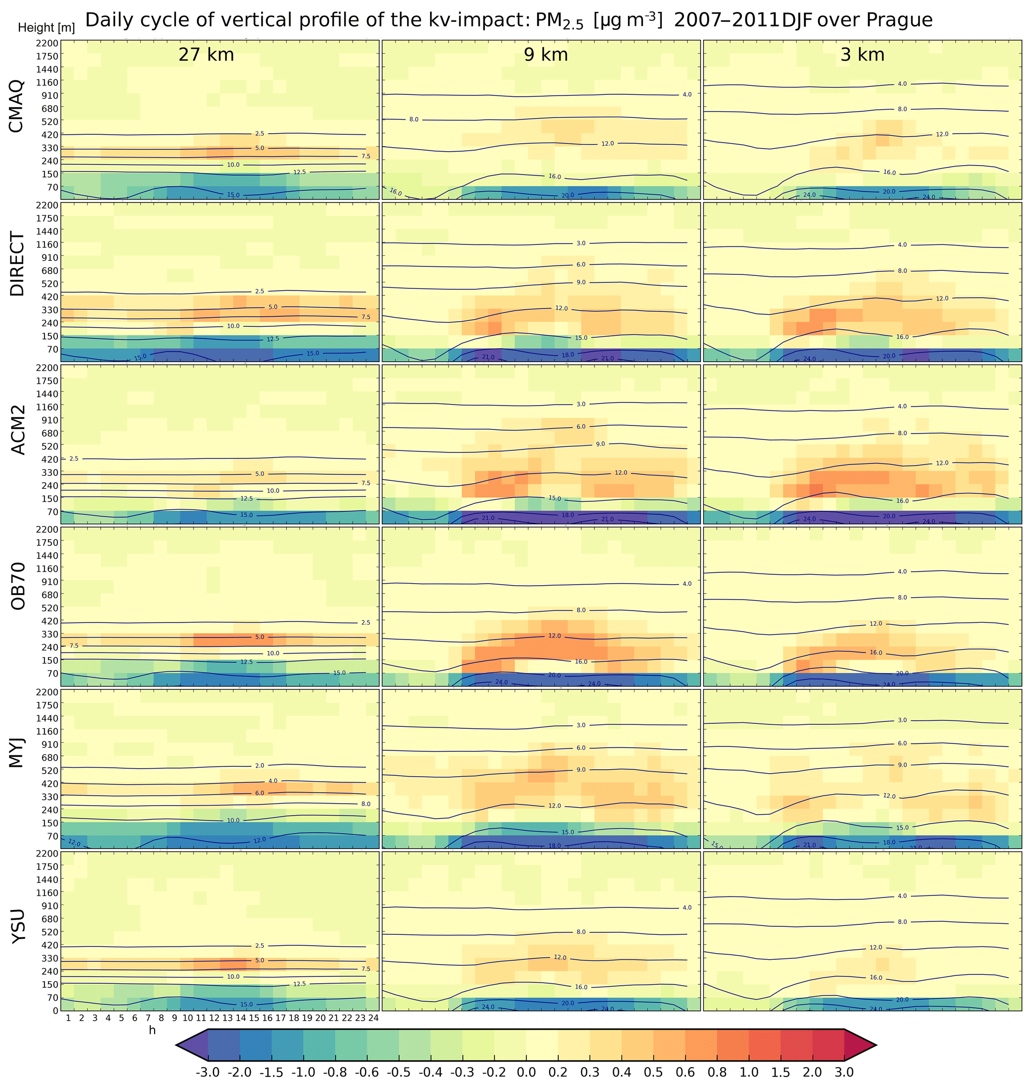
Figure 27 presents the absolute K_v values and the kv-impact for DJF for Prague. It is clear that the 9 and 3 km resolutions result in higher near-surface concentrations and the vertical spread of the PM_2.5 is stronger than that at 27 km. Regarding the impact, it reaches higher values in the 9 km and 3 km resolutions, and the maximum kv-impact is reached for the DIRECT, ACM2 and OB70 methods (up to −3 µg m⁻³ decrease) during daytime. For the 27 km resolution and for the YSU and CMAQ methods, the PM_2.5 decrease is smaller (up to about −1 µg m⁻³). Similar to Berlin, the PM_2.5 increase and higher levels are evident too and are stronger for the 9 and 3 km resolutions. They occur between 150 and 400 m, and reach 0.8–1 µg m⁻³, especially for the DIRECT, ACM2 and OB70 methods.

3.3.2 The total urban impact

One of the most important questions to answer in this paper concerns the dominance of enhanced turbulence within the urban canopy impact on air quality via the urban meteorological effects. To answer this question, we evaluated also the total- or the t+q+uv+kv-impact for both analyzed pollutants as the difference between the URB_t+q+uv+kv and NOURBAN simulations for each resolution. As the NOURBAN model experiment is calculated using only the CMAQ K_v method; the total-impact is given also only for this method. Here, based on short 1-month test simulations, we verified that the t-, q- and uv-impacts depend on the choice of the K_v calculation only weakly (in contrast to the kv-impact itself, which is strongly dependent on the choice of the K_v scheme).

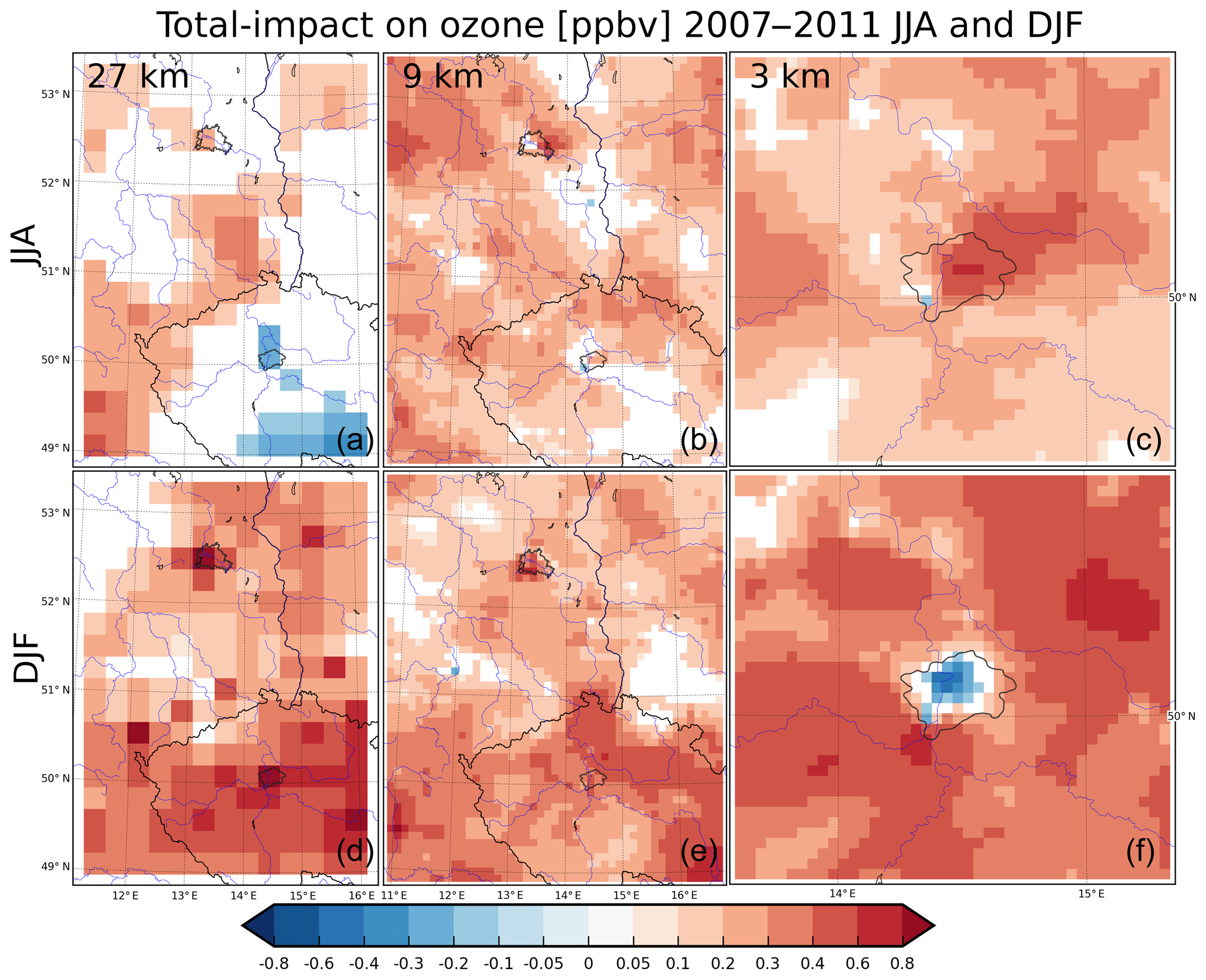
Figure 28 The total impact of urban meteorological changes (i.e., temperature, humidity, wind and vertical eddy diffusivity) on surface O₃ concentrations in ppbv for the 27, 9 and 3 km resolutions (left to right) for JJA (a, b, c) and DJF (d, e, f). Shaded areas represent statistically significant changes on the 98 % threshold level using a two-tailed t test. The default CMAQ K_v method was invoked in this calculation. The geographic locations of Berlin and Prague are indicated by their administrative boundaries.

Figure 28 presents the total-impact of the urban meteorological changes on the mean canopy concentrations of O₃ for each resolution and both seasons. Huszar et al. (2018a) predicted that near-surface O₃ should increase due to the increased removal (turbulent dispersion) of NO_x from urban areas and thus reduced titration, as well as due to enhanced turbulent transport from higher levels, although they pointed out that the overall effect is always a result of competitive impact of multiple influences. Indeed, in our results, ozone usually increases too, but the magnitude of the increase changes substantially across resolutions, and it is different for the two cities. For Berlin, it reaches around 0.2–0.3 and 0.4–0.6 ppbv for the 27 and 9 km simulations, respectively. For Prague, increases are encountered for the 9 and 3 km resolutions, reaching 0.3 and 0.8 ppbv, respectively. However, for the 27 km simulation, the overall urban impact turns out to be negative (about −0.2 ppbv). During DJF, ozone increases over both cities, mostly for the 27 km resolution (reaching 0.8 ppbv). However, for Prague, in the 3 km resolution, O₃ decreases (up to −0.6 ppbv), in contrast to the JJA results.

Figure 29 The diurnal cycle of the absolute ozone concentrations (solid; left-hand axis) as well as the total-impact (i.e., the t+q+uv+kv-impact; dashed; right-hand axis) above Berlin (a, c) and Prague (b, d) for JJA (a, b) and DJF (c, d) in ppbv. Red, orange and green colors stand for 27, 9 and 3 km resolutions, respectively.

In order to see whether the simulated total-impact is uniform during the day or if it behaves qualitatively and quantitatively differently during different hours, we plotted further the diurnal cycle of this impact along with the absolute concentrations for both cities and seasons, as shown in Fig. 29. For JJA, the absolute values (solid lines) are in line with the expectation of maximum during afternoon, while the difference between the different resolutions is not greater than 6–8 ppbv (greatest differences in the daily maxima and nighttime values). The impact (dashed lines) is characterized by a clear main maximum during afternoon hours reaching 3 ppbv for Berlin, while it is less pronounced in the coarse-resolution simulation. A secondary maximum is visible too during morning hours, especially for Prague. The minimum of the impact is encountered during early afternoon, and here, the differences between the resolutions are very large for Prague, ranging from −2 ppbv to almost 0, explaining the overall negative impact of the urban canopy meteorological forcing on ozone in the previous figure. During DJF, absolute ozone concentrations encounter two maxima: one during early morning and one during early afternoon. In DJF, ozone titration is the dominant process in cities, while ozone is transported here by turbulence from upper levels. The titration rate is highest when NO_x emissions are peaking and this occurs in the morning and late afternoon, putting the two ozone maxima in between. In general, the 9 and 3 km resolutions result in higher absolute ozone for this season, especially during nighttime. The total-impact is, again, characterized by a clear late afternoon maximum reaching 2–3 ppbv and being strongest in the 27 km simulation. It is present also in the 3 km simulation for Prague; however, a negative peak forms here during morning (reaching −1.5 ppbv), which results in the overall negative impact on ozone seen in Fig. 28.

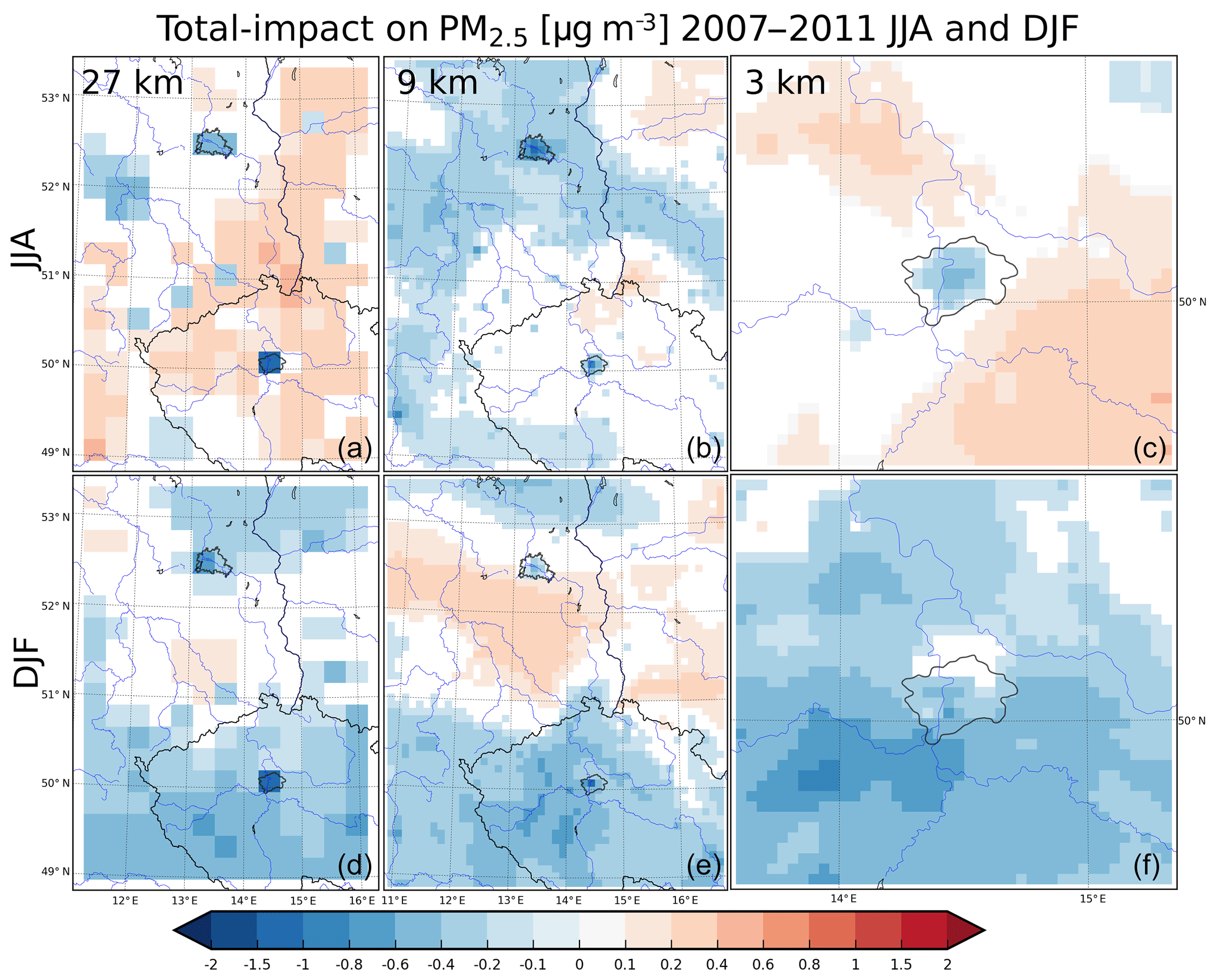
Figure 30 The total impact of urban meteorological changes (i.e., temperature, humidity, wind and vertical eddy diffusivity) on surface PM_2.5 concentrations in ppbv for the 27, 9 and 3 km resolutions (left to right) for JJA (a, b, c) and DJF (c, e, f). Shaded areas represent statistically significant changes on the 98 % threshold level using a two-tailed t test. The default CMAQ K_v method was invoked in this calculation. The geographic locations of Berlin and Prague are indicated by their administrative boundaries.

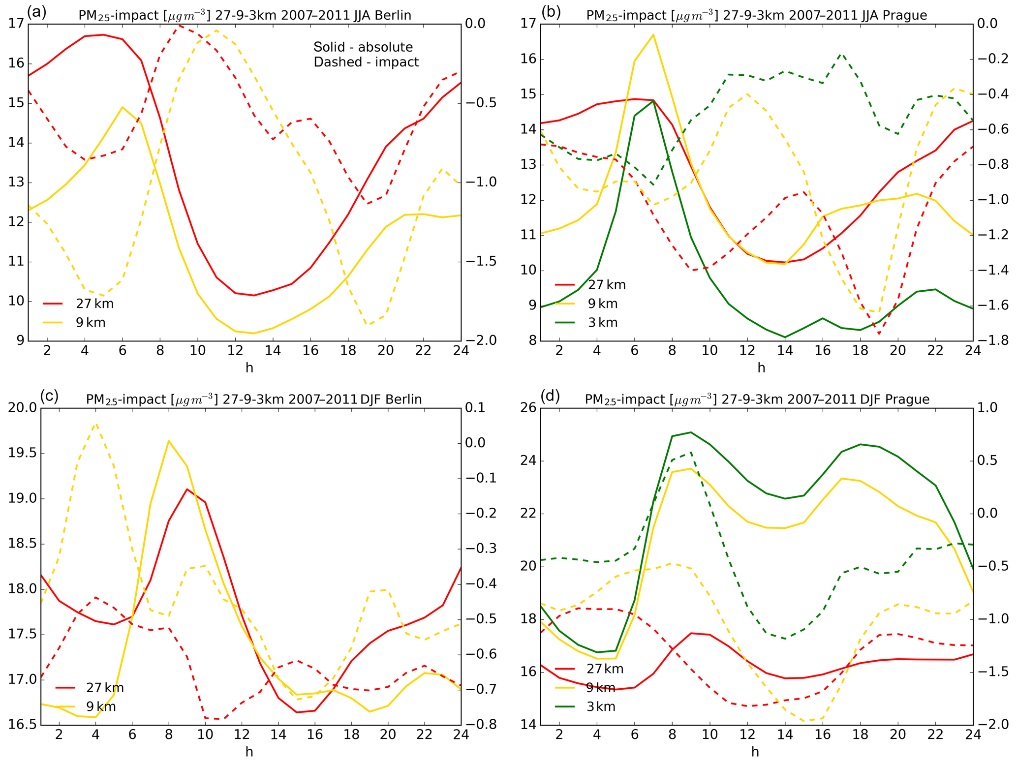
Figure 31 The diurnal cycle of the absolute PM_2.5 concentrations (solid; left-hand axis) as well as the total-impact (i.e., the t+q+uv+kv-impact; dashed; right-hand axis) above Berlin (a, c) and Prague (b, d) for JJA (a, b) and DJF (c, d) in µg m⁻³. Red, orange and green colors stand for 27, 9 and 3 km resolutions, respectively.

The total-impact on PM_2.5 surface concentrations is presented in Fig. 30. The impact is negative in all cases, confirming the expectations that the effect of turbulent removal dominates (Huszar et al., 2018b). However, the magnitude of the change varies greatly between the cities and resolutions. It reaches −1.5 to −2 µg m⁻³ for Prague in both analyzed seasons and is strongest at 27 km resolution, while at 3 km, the decrease is only about −0.6 µg m⁻³. Over Berlin, the decrease is in the range of −0.4 to −1 µg m⁻³; in JJA, it is slightly stronger in the 9 km simulation, while in DJF, the opposite holds.

The diurnal cycle of the absolute near-surface PM_2.5 concentrations as well as the total-impact over Berlin and Prague is presented in Fig. 31. A clear maximum occurs in the absolute values in JJA during morning hours over both cities, in line with the emissions' temporal evolution, while the difference between individual resolutions is within 5 µg m⁻³ and is highest during nighttime when the 27 km simulation produces the largest concentrations. Regarding the total-impact, in JJA, there is a clear negative peak during evening hours for both cities, reaching −2 µg m⁻³. However, at 3 km resolution, this peak is less pronounced and reaches only about −0.6 µg m⁻³. Here, another peak is present during morning hours and this is seen also at 27 and 9 km resolutions, especially for Berlin. During DJF, absolute concentrations exhibit a main maximum during morning hours, while a secondary peak is present during evening hours, probably in connection with the diurnal cycle of the emissions. The diurnal cycle of the impact is very similar between individual resolutions and cities with one main peak during morning hours when the impact is the smallest (it almost disappears over Berlin at 9 km resolution). Later, the impact increases, during noon to afternoon hours, reaching −2 µg m⁻³, similarly to the JJA impact. Again, the smallest impact is modeled at 9 km resolution (about −1 µg m⁻³).

In summary, when comparing the individual resolutions, it is clear that the total-impact for both O₃ and PM_2.5 can vary largely, in both the quantitative and qualitative sense. Further, it is evident that the kv-impact (evaluated in the previous section) will add further uncertainty to the results, as its spread is even larger than the spread seen in the total-impact due to different resolutions (bear in mind that the kv-impact represents a major component of the total impact). Further, the total-impact was evaluated using the CMAQ method. This resulted in one of the smallest kv-impacts. Even as such, it clearly dominates the total-impact. Consequently, using other K_v methods would lead to even stronger total-impact (increase of ozone and decrease of PM_2.5) and thus confirms the dominance of the modifications in vertical turbulent transport among other components of the urban canopy meteorological forcing.

4 Discussion and conclusions

The validation of model results showed a clear overestimation of winter temperatures in RegCM, along with a precipitation overestimation. Previously, Giorgi et al. (2012) reported this positive bias too using the same PBL scheme (UW scheme). Along with the positively biased winter temperatures, this suggests that the heat removal from the surface towards higher levels is probably underestimated (in contrast to the older HOL scheme), and this leads to higher surface temperatures. Large positive rain bias was shown also in Huszár et al. (2016b), and they attributed it to overestimation of cloudiness which, in winter, can lead to positive temperature bias due to reduced radiative cooling of the surface. In summer, the results are more mixed but the model stays within a reasonable range compared to observations.

The comparison of modeled pollutant concentrations with observations showed several model deficiencies. For ozone, it is especially the strong overestimation of the nighttime values (while daytime peaks are reasonably captured), which in turn leads to underestimation of the diurnal amplitude. This was commonly encountered in regional climate chemistry studies (Zanis et al., 2011; Huszar et al., 2016a; Karlický et al., 2017). For example, Zanis et al. (2011) found that nighttime ozone values are captured in the model (they used CAMx too) with less accuracy than daytime ones and argue that this is caused by more stable conditions when ozone values are more sensitive to the vertical profiles of meteorological variables, emissions and the precursor concentrations. It is clear that, in the future, more emphasis should be put on processes determining nighttime surface ozone, as improving the nighttime model accuracy will yield a more reasonable starting point for the development of daytime ozone (Wong and Stutz, 2010) and an overall better model performance. The positive nighttime ozone bias results in overestimated monthly ozone.

Higher model ozone may suggest that some of the urban impacts on this gas may be slightly overestimated, assuming that the impact increases with increasing absolute values. It is also evident from the results that higher resolutions did not bring substantial improvement to model accuracy (except that the daily ozone maxima are captured with a higher accuracy in the 3 km model runs). The same conclusion was recently stated by Falasca and Curci (2018), who applied WRF over Italy at similar (cascading) domain resolutions. It also evident from the absolute values of concentrations in the ozone diurnal cycle figures that K_v methods produce higher diffusivities (compared to the default one), resulting in higher ozone values (e.g., the TKE-based methods), which is due to higher NO_x turbulent removal in cities and therefore lower ozone titration. This means that the positive ozone bias will be even higher. This, however, does not mean that these methods are erroneous, as the model bias has in general multiple causes (inaccurate diurnal profile of emissions, biased nighttime chemistry, etc.) rather than one particular process (vertical eddy diffusion).

Regarding PM_2.5, the most important model shortcoming is the strong underestimation of observed values during winter, especially over urban stations. On the other hand, overestimation occurs in summer, especially for the 27 and 9 km domains. Many stations from western Europe were included in the validation, and these showed systematic model overestimation also in Huszar et al. (2018b) and outweighed the underestimation seen for other central European countries, especially Czech Republic, which encompasses the whole 3 km domain. Note that the emission data used in this study are basically a new version of those used in the former study and differ only slightly. The REZZO/ATEM emissions used for Czech Republic are also quantitatively very similar to the TNO data over this country too. Huszar et al. (2016a), using similar model resolution and emission data, showed similar large DJF underestimations of PM_2.5 and attributed them to underestimated nitrate aerosol and black/organic carbon. Myhre et al. (2006) and Schaap et al. (2004) encountered similar negative bias for these aerosol components. Further, we see that using the other K_v calculation method which produces stronger diffusivities will result in higher turbulent removal of PM_2.5 from near the surface, resulting in more pronounced negative bias. However, similar to the case of ozone, this does not imply that these “stronger” K_v schemes are wrong, as, again, the model bias has multiple components (and here most probably caused the bias in the secondary aerosol formation). In such cases, improving model physics can often lead reduced model accuracy.

In summary, a weak sensitivity of modeled concentrations to the resolution of the driving meteorological as well as CTM is seen, as concluded earlier by Markakis et al. (2015), who performed similar climate-driven air quality simulations over Paris (France). Indeed, the largest uncertainty of modeled concentrations is associated with emissions, especially over urban areas (Aleksankina et al., 2019); however, recall that in our case, emissions were kept constant and only the uncertainty of the representation of urban boundary layer was analyzed.

The average urban canopy impact on temperature is very similar to the values presented in Huszar et al. (2018a) who, for the two analyzed cities (Berlin and Prague), encountered increases up to 1.5–2 ^∘C. The diurnal variation of the impact shows also large similarities in both the quantitative and qualitative sense, when the maximum impact occurs around late evening. The urban impact on temperature is consistent with previous observation (Gaffin et al., 2008) and model-based studies (Pichierri et al., 2012; Giannaros and Melas, 2012; Struzewska and Kaminski, 2012), while Sarrat et al. (2006) simulated somewhat later timing of the maximum urban impact. Our simulations, extended to winter, suggest that the magnitude of the impact remains similarly high during winter and here probably the effects of anthropogenic heat dominate over the radiative and thermal effects associated with radiation trapping (Karlický et al., 2018; Varentsov et al., 2018; Halenka et al., 2019). Although increased resolution results in spatially more detailed impact, with maximum temperature increases concentrated in the city center (seen especially for Prague in the 3 km simulation), there is no systematic effect of the choice of resolution. The impact, however, strongly depends on how the model grid covers a particular city and if the city center matches a grid point (Prague) or if it lies in between (Berlin). This suggests that efforts should be made to adapt the grid to the geographic location of city centers which is best achieved by choosing multiple disjunct nested domains under the parent grids (e.g., as in Wang et al., 2012).

The impact on average wind speed with values up to −2 ms⁻¹ matches previous studies too. For example, Struzewska and Kaminski (2012) simulated similar reductions for central European cities, but Chinese cities in Zhu et al. (2017) encountered comparable decreases too. Compared to the decreases in Huszar et al. (2018a), reaching −1 ms⁻¹, our results suggest that, in the event of wind, higher resolutions bring stronger impact. Indeed, the 27 and the 9 km impacts are always less than the 3 km result for Prague. This indicates that higher resolutions yield stronger peak wind modifications in city centers. A sudden decrease (in the absolute sense) of the wind impact during evening hours is visible in our simulations too and is probably connected to the evening PBL transition (Lapworth, 2003). The wind impact during winter turned out to be somewhat larger than that in summer, which is connected to more stable stratification when less turbulence is present (see further) and less momentum is transferred to the surface from above the PBL. The timing of both the minimum and maximum urban canopy wind speeds (as well as those of temperature) is in very good agreement with Zhang and Zheng (2004).

Our results suggest a large sensitivity of the modeled vertical eddy diffusivities to the choice of the method for its calculation, and the same is true for the urban-canopy-induced changes. Near-surface K_v modifications range from 0.5 to as much as 30 m² s⁻¹. Over higher model levels, the impact spans 2 orders of magnitude, i.e., 1 to 100 m² s⁻¹, comparable to the range of absolute values themselves. The TKE-based methods systematically generate higher K_v values; this is in line with Kim et al. (2015), who compared a improved version of MYJ used here and the YSU scheme. They concluded that MYJ generates stronger vertical mixing at about 400–500 m above the surface than the YSU scheme, although the depth of the PBL was larger in YSU in their simulations. Our K_v values for the CMAQ method are in good agreement with the values of Huszar et al. (2018a) calculated using the same method. Kim et al. (2015) predicted a K_v increase due to application of the urban canopy scheme up to 100 m² s⁻¹ (same as in our study), and the height of the maximum increase coincides well with our results too. In Environ (2011), OB70 and YSU methods generated the smallest K_vs too, in line with our results. However, they predicted K_v values for the MYJ methods comparable to CMAQ (and comparable to our CMAQ values), in contrast to our results. This could suggest that the TKE from which K_v is derived is somewhat overestimated in our RegCM simulations.

The resolution seems to have rather minor impact on the result near the surface. However, a finer resolution results in stronger impact at higher elevations. This seems to be true for both the absolute diffusivities as well as for the urban canopy impact. Regarding the difference between winter and summer, in winter, absolute K_v values are lower, as expected from the more frequent stable stratification. The urban canopy impact on K_v at higher levels is stronger in summer; however, at the surface, the difference between summer and winter is rather small. The maximum K_v impact is simulated in all diffusion schemes during early evening. This is related to the evening PBL transition when urban PBL height decreases more slowly than the rural one, resulting in a relatively large urban–rural difference and hence a large impact on K_v (Pal et al., 2012).

The simulated changes in the vertical eddy diffusion coefficient alone led to ozone increases, as expected from the previous studies of Sarrat et al. (2006) and Kim et al. (2015). NO_x is removed from the surface layer more efficiently over urbanized areas, leading to reduced ozone titration, while at the same time the increased transport from the residual layer during nighttime is contributing too, as shown by Huszar et al. (2018a). They used the CMAQ method for K_v calculation and simulated (for JJA) a higher ozone increase up to 3 and 2 ppbv over Berlin and Prague, respectively, compared to our CMAQ results of about 1.5 and 0.8 ppbv for Berlin and Prague. Higher kv-impact on ozone (up to 4 ppbv) is simulated with the TKE-based methods, but comparable magnitude is achieved also with the ACM2 and OB70 approaches. It is not clear whether higher resolutions lead to systematic change of the urban core kv-impact. Often, the middle resolution (9 km) exhibits the largest value. Interestingly, the kv-impact for OB70 is one of the strongest; the urban-canopy-induced K_v modifications were at the low end in the case of this method. This is also true for the ACM2 method, for which the K_v modifications were far from the strongest; however, this propagated to almost the strongest impact on near-surface ozone. The impact during winter is somewhat stronger than that in summer. This is probably due to higher reduction of NO_x–ozone titration in winter caused by NO_x turbulent dispersion. Again, the CMAQ and YSU methods generate weakest ozone changes. In summary, the simulated range of K_v changes of about 0.5 to 30 m² s⁻¹ was propagated to a range of the kv-impact near the surface of about 0.6 to 4 ppbv. The vertical profile of ozone changes further showed decreases at higher levels. This is probably due to NO_x being removed from the surface, causing titration at higher levels, but the increased transport from RL can contribute too. Zhu et al. (2015) showed that in urban plumes, ozone is increased in the upper boundary and decreased in the lower one. Our results exhibit a small increase of ozone at higher levels and the mentioned decrease often extends to the lower boundary layer, putting our results in line with theirs. The range of elevated ozone decreases due to different K_v methods is relatively large, spanning from −0.4 to −2 ppbv.

The response of PM_2.5 concentrations to urban-canopy-enhanced vertical turbulent transport predominantly shows decreases due to the dominance of dispersion by increased eddy diffusion (Zhu et al., 2017; Kim et al., 2015). Huszar et al. (2018b), however, showed that individual aerosol components react differently to increased eddy transport and secondary aerosols can even increase slightly, although the decrease of the primary aerosols shaped the total PM_2.5 response. Our results suggest PM_2.5 decrease from a few tenths up to −1 µg m⁻³ in summer and even stronger decrease (up to −2 µg m⁻³) in winter, which is – at least for summer – quantitatively close to Huszar et al. (2018b), who simulated summer decreases for Berlin and Prague up to −2 and −1 µg m⁻³, respectively. The decreases due to urban-canopy-induced K_v enhancement in Kim et al. (2015) are somewhat larger, but this can be due to different chosen city (Paris). Our results indicate that, in connection with K_v enhancement, even increases can occur. This is probably due to the fact that the aerosol removed from the surface level to the upper ones is transported to other regions where it is deposited back to lower levels outweighing the turbulence-enhanced local reduction. This effect is expected to be strong over a larger domain, where the simulation allows the aerosol to be transported to larger distances. Indeed, our 27 km domain results show some PM_2.5 increase, especially over rural areas but also for Berlin. Our results further showed that the winter PM_2.5 decreases are larger, which is in line with the fact that the winter urban-canopy-induced K_v increases are higher too. Comparing the individual K_v methods, it is seen that the strongest impact is simulated by the ACM2 scheme, but the OB70 and the TKE-based schemes are comparably strong too. On the other hand, the default CMAQ scheme generates a much weaker impact along with the YSU scheme. Kim et al. (2015) concluded too that the MYJ scheme resulted in a larger impact on PM than the YSU. We also found that during summer the strongest impact is modeled during afternoon/evening hours, reaching −3 µg m⁻³, in line with Huszar et al. (2018b). The choice of the K_v method, however, strongly determines the shape of the diurnal cycle of the impact, especially in summer.

The total urban canopy impact (i.e., the combined impact of temperature, humidity, wind and turbulence) exhibited a relatively large range of values for ozone from −0.6 to 0.8 ppbv, depending on the resolution and season. This underlines the fact that the total-impact encompasses multiple components that act simultaneously and have opposite signs (Huszar et al., 2018a). This includes both reductions (due to increased $\mathrm{NO}+{\mathrm{O}}_{\mathrm{3}}\to {\mathrm{NO}}_{\mathrm{2}}$ reaction and increased dry deposition) and increases (due to vertical turbulent removal of NO_x from the near surface where it causes titration). Over Prague, the wind and the temperature impact in winter was evaluated to be relatively large, while the CMAQ impact on K_v was small. As the total-impact was evaluated only for this K_v method, this suggests that decreases due to increased temperature and decreased wind speeds will be strong, and indeed, they apparently outweighed the impact of enhanced turbulence leading to concentration decrease, especially over the fine-resolution domain. However, when we compare these results to the much stronger kv-impact gained by other K_v methods, we clearly see that using them would turn the impact into a positive one, making the turbulence changes again a dominant factor shaping the total-impact. We can conclude here that the vertical eddy diffusion is a dominant factor that determines the impact of urban canopy forcing on ozone; however, there is relatively large uncertainty given how K_v values are calculated, and under certain conditions this dominance is not clear or can be even slightly overweighed by opposite effects.

In the case of the total impact on PM_2.5, the dominance of enhanced turbulence is clear for each resolution, city and season, although the magnitude covers a wide range, from a few tenths up to −2 m² s⁻¹. As already said, the CMAQ method was used to calculate the total impact, and again, the PM_2.5 change due to kv-impact calculated using this method turned to be one of the smallest. We can thus conclude here that using other methods would lead to even larger decreases of PM_2.5 due to the total urban impact, confirming the dominance of enhanced vertical eddy transport over urban areas.

In summary, our results confirm that turbulence is a prominent factor that determines the impact of urban canopy meteorological forcing on the urban air quality. In the case of ozone, it leads to increased concentrations, while PM_2.5 responds with decreases. This holds for both summer and winter seasons. Finally, model resolution seems to play a rather minor role, and the effect of urban-canopy-induced modifications of vertical eddy diffusion is dominant in both coarse- and high-resolution model simulations. Our study demonstrates the dominant role of turbulent transport of pollutants above urban areas and stresses the need for further investigation of how variation of urban land use (within urban mitigation and adaptation strategies) influences the pollutant transport from the urban canopy to the whole urban PBL.