Source backtracking for dust storm emission inversion using an adjoint method: case study of Northeast China

Emission inversion using data assimilation fundamentally relies on having the correct assumptions about the emission background error covariance. A perfect covariance accounts for the uncertainty based on prior knowledge and is able to explain differences between model simulations and observations. In practice, emission uncertainties are constructed empirically; hence, a partially unrepresentative covariance is unavoidable. Concerning its complex parameterization, dust emissions are a typical example where the uncertainty could be induced from many underlying inputs, e.g., information on soil composition and moisture, land cover and erosive wind velocity, and these can hardly be taken into account together. This paper describes how an adjoint model can be used to detect errors in the emission uncertainty assumptions. This adjoint-based sensitivity method could serve as a supplement of a data assimilation inverse modeling system to trace back the error sources in case large observation-minus-simulation residues remain after assimilation based on empirical background covariance.

The method follows an application of a data assimilation emission inversion for an extreme severe dust storm over East Asia (Jin et al., 2019b). The assimilation system successfully resolved observation-minus-simulation errors using satellite AOD observations in most of the dust-affected regions. However, a large underestimation of dust in Northeast China remained despite the fact that the assimilated measurements indicated severe dust plumes there. An adjoint implementation of our dust simulation model is then used to detect the most likely source region for these unresolved dust loads. The backward modeling points to the Horqin desert as the source region, which was indicated as a non-source region by the existing emission scheme. The reference emission and uncertainty are then reconstructed over the Horqin desert by assuming higher surface erodibility. After the emission reconstruction, the emission inversion is performed again, and the posterior dust simulations and reality are now in much closer harmony. Based on our results, it is advised that emission sources in dust transport models include the Horqin desert as a more active source region.

1 Introduction

Severe dust storms are relatively common events in arid or semi-arid regions over the globe, e.g., in North Africa, the Middle East, Southwest Asia and East Asia, and Australia (Shao et al., 2013). Dust particles could be lifted several kilometers high into the atmosphere and subsequently carried over distances of thousands of kilometers by the prevailing winds. Substantial amounts of dust particles in dust storms are a great threat to human health and properties in areas downwind of dust source regions (World Meteorological Organization, 2018; Basart et al., 2019). The impact on human health consists of dust pneumonia, strep throat, cardiovascular disorders and eye infections. Dust storms can also carry irritating spores, bacteria, viruses and persistent organic pollutants (World Meteorological Organization, 2017). Next to human health, the resulting low visibility can cause a severe disruption of the transportation system. For instance, struck by a choking dust storm, visibility in Beijing plummeted, and over 1100 flights were delayed in early May 2017 (Jin et al., 2019b). The dust cycle itself is also a key player in the Earth system, with profound effects on terrestrial and ocean fertilization, precipitation (Benedetti et al., 2014) and atmospheric radiation (Kosmopoulos et al., 2017).

Due to the growing interest in dust storms, the understanding of the physical processes associated with the dust cycles has increased rapidly over the last decades (Ginoux et al., 2012; World Meteorological Organization, 2018). To improve the simulation skill of dust models, many studies were carried out to parameterize the emission rates using wind tunnel tests or field experiments (Shao et al., 1996; Marticorena and Bergametti, 1995; Alfaro et al., 1998; Fécan et al., 1999). These emission parameterization schemes were then incorporated into large-scale global chemical transport models, e.g., CAMS-ECMWF (Morcrette et al., 2009), or regional ones, e.g., NASA-GEOS-5 (Colarco et al., 2010) and BSC-DREAM8b (Basart et al., 2012). An important application of these models is to forecast dust concentrations over a few hours to a few days in order to reduce the potential impact on society (Wang et al., 2000; Gong et al., 2003). Different from anthropogenic aerosols, dust particles arise from a complex erosion process with extremely high spatial and temporal variability. A crucial element for the correct simulation (and forecast) of dust transport is the correct representation of the source areas and emission rates. In large-scale modeling systems, this representation remains relatively crude, due to uncertainty in the different input data such as soil properties (most importantly soil texture data), surface roughness, land cover (vegetation), topography, as well as insufficient knowledge about the aerosol lifting process itself (Escribano et al., 2016). Besides, quality of forecast of relatively coarse resolution models for wind fields and soil moisture can impact prognostic quality of dust emission and transport. The difficult task of describing all of these inputs correctly subsequently leads to nontrivial simulation errors. Large discrepancies (a factor of up to 10) in dust emissions among models were reported in the evaluation of multiple models participating in the Aerosol Comparison between Observations and Models (AeroCom) phase I experiments (Huneeus et al., 2011; Koffi et al., 2012); the observation-minus-simulation difference can even be as large as 2 orders of magnitude (Uno et al., 2006; Gong and Zhang, 2008).

Recent advances in sensor technology and the reduced cost of monitoring systems have led to an increase in observation data that could be used to analyze dust storms. These observations could be used to explore and improve aerosol emission simulation through inverse modeling. Progress in dust emission inversion has been made in the last decade by assimilating column-integrated satellite aerosol properties (e.g., Moderate Resolution Imaging Spectroradiometer (MODIS) in Schutgens et al., 2012, Khade et al., 2013, Yumimoto and Takemura, 2015, Yumimoto et al., 2016a, Di Tomaso et al., 2017, and Himawari-8 in Jin et al., 2019b), Cloud-Aerosol LIdar with Orthogonal Polarization (CALIPSO) vertical aerosol profiles in Sekiyama et al. (2010), and ground-based PM₁₀ concentrations (Jin et al., 2018, 2019a).

Most of these dust emission inversion systems use variational methods to estimate the optimal emissions. Since a large programming effort is required to formulate and implement the tangent linear (TL) model and its adjoint model (AM) in the traditional 4DVar, those systems often employ model-reduced or ensemble-based variational assimilation. With model reduction, a simplified tangent-linear model is used to propagate the background error covariance. Ensemble methods generate an ensemble of perturbed emissions and propagate this ensemble to approximate the evolution of background error covariance. Both of these adjoint-free methods are able to reduce uncertainty in emissions by determining the dominant and sensitive patterns. The computation costs necessarily limit the size of the reduced tangent-linear model or the size of the ensemble to a number that is much smaller than the size of the emission parameter space. Consequently, the optimal emissions that can be calculated are constrained to a subset of the original space, which is defined by the model or parameter reduction that was applied.

A crucial element of all inversion methods is the proper specification of the spread in possible estimates, which is in this application the spread in possible emissions. Ideally, the emission uncertainties should be both physically reasonable and capable of providing sufficient variations to explain the observation-minus-simulation differences. Unfortunately, the many possible errors that could be present in dust emission parameterizations could not be described all together, and simplifications are needed. Many studies use fairly coarse emission uncertainty, limited to optimization of a few scaling factors for emission inventories spanning a larger domain. For example, in the dust emission inversion research by Yumimoto et al. (2008), the emission background covariance is assumed to be uncorrelated in space, and the uncertainty is simply defined as 500 % of the prior emission flux rate. Khade et al. (2013) introduced an uncertain erodibility fraction parameter field to introduce variability in dust emissions over the Sahara and reduced the uncertainty by using an ensemble adjustment Kalman filter (EAKF). Di Tomaso et al. (2017) attributed the emission error to the uncertainty in the friction velocity threshold (FVT), which was reduced by estimating an optimal correction factor using a local ensemble transform Kalman filter (LETKF). Limited by the ensemble size, the multiplicative value was considered spatially and temporally constant. In a previous study described in Jin et al. (2018), a spatially varying multiplicative factor was applied to compensate for the errors in the FVT in the dust emission parameterization. More recently in Jin et al. (2019b), the uncertainties were described by including uncertainty in the FVT and in the surface wind field.

An essential step before starting an inversion is to check whether the specified uncertainties are actually able to explain the differences between observations and simulations. The sensitivity of the model with respect to the uncertainties should learn whether the parameters considered are really the dominant problematic parameters. Under the circumstances that the aforementioned model-reduced or ensemble-based variational data assimilation algorithms are adopted, the knowledge of the sensitivity is particularly valuable, since it can efficiently help the model/parameter reduction by removing those insensitive problematic parameters. Based on this knowledge, the background covariance could be improved, which will immediately improve the emission inversions.

An efficient way of examining sensitivities is the use of an adjoint model. This is especially useful for examining the sensitivity of a limited number of output values for changes in a large amount of input values. The first implementations of an adjoint of an atmospheric transport model were in the early 1980s with applications in numerical weather forecasting (Dimet and Talagrand, 1986; Talagrand and Courtier, 1987). Implementations in chemical transport models (CTMs) can be found in Elbern et al. (1997), Hakami et al. (2005), Hourdin and Talagrand (2006), Henze et al. (2007b), and An et al. (2016). The standard forward version of a CTM requires input from initial conditions and model parameters and provides concentrations in receptor points as output. The state evolution could therefore be regarded as source-oriented. Adjoint models, however, could be regarded as receptor-oriented, as they use a distortion in a receptor point as input and compute from this the distortions of the input parameters that explain this. In case of many uncertain parameters, an adjoint model is very efficient in calculating model sensitivities than other methods such as the traditional finite-difference method, which requires many forward model runs with perturbed inputs (Zhai et al., 2018).

In this study, we first review the emission inversion conducted in Jin et al. (2019b), where the Himawari-8 satellite AOD observations were assimilated for a dust storm event in May 2017. Although significant improvements in dust simulation and forecast skills driven by the posterior emissions were reported, some large regional simulation errors remained. In particular, during three severe dust (SD) outbreaks, some high dust concentrations observed at ground level were not at all or not completely resolved by the a posteriori simulations, although the assimilated AOD observations also indicated that a severe dust plume was present. An adjoint version of the transport model is then introduced. It will not be used to optimize emissions (although that would make sense in a 4DVar context); instead, it is used to trace back the potential emission source that could explain the observed high concentrations. For the three selected dust outbreaks the sensitivity towards the emissions is computed for observation sites that were not resolved correctly by the assimilation. Each of the results pointed to the Horqin desert as the most likely source region for this event. The Horqin desert, which is also named the Horqin sandy land, is mixed with sparse vegetation and agriculture lands in northeastern China. Though it is recognized as one potential emission source in several dust models, it is also considered of far less importance compared to other major ones, e.g., the Gobi and Mongolia deserts and Taklamakan desert (Zhang et al., 2003; Ginoux et al., 2012; UNEP, WMO, and UNCCD, 2016). Kim et al. (2013) suggested a dynamic vegetation index is essential for representing the seasonal bareness variation that regulates dust emissions over this region. Zhang et al. (2016) predicted a declining trend in dust emission from this sandy land due to the climate change. For LOTOS-EUROS used in this work and another model, BSC-DREAM8b, it is not present as an easily erodible in the dust emission scheme, at least for these tested severe events. To evaluate whether dust emissions from the Horqin desert could indeed explain the observed high concentrations, a new inversion is applied with a modified emission model with a higher surface erodibility over this region. The new reference model is further improved by assimilating ground-based PM₁₀ observations, which significantly reduce the remaining differences.

While various studies on aerosol and/or dust emission inverse modeling assume that the locations of sources are known, this study represents application of this methodology in detecting dust source areas which are still not recognized as sources with a significant contribution to the airborne dust cycle. Within this context, the highlights are 2-fold. First, this study shows how an adjoint model could be used to identify potential sources in case large observation-minus-simulation error residues are found that cannot be explained by the existing model and assumed or empirical uncertainties and thus cannot be corrected using a data assimilation system. With the potential source region identified by the adjoint sensitivities, the background emission uncertainty is updated. Second, although the existing emission scheme worked properly in most deserts in East Asia, e.g., Gobi and Mongolia, it highly underestimated the possible emissions from the Horqin desert. Based on our results, it is advised that emission sources in dust transport models include the Horqin desert as a more active source region.

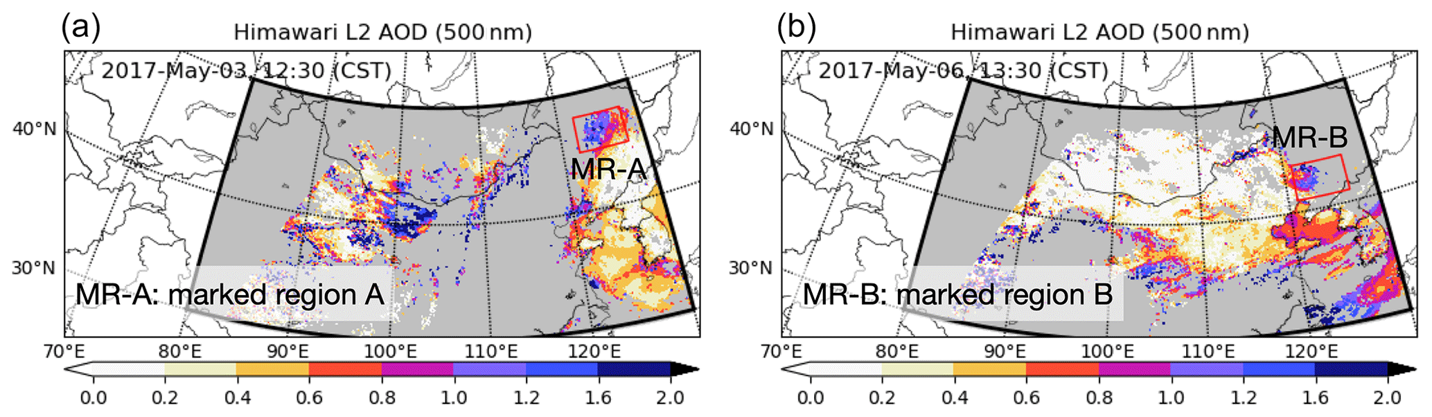
Figure 1 Two snapshots of Himawari-8 Level 2 AODs (500 nm) on 3 May, 12:30 and 6 May, 13:30. Note that only observations within the black framework are included, where gray values denote pixels for which no AOD was retrieved.

This paper is organized as follows. Section 2 introduces the measurements, the Himawari-8 AOD and the ground-based PM₁₀ observations that are used in this study. Section 3 mainly discusses the numerical dust transport model, the various causes of simulation emission errors, and the difficulties in accurate emission uncertainty quantification. Section 4 presents the theory of adjoint modeling and evaluates the accuracy of adjoint sensitivity. Section 5 reviews the emission uncertainty construction that was used in the previous study (Jin et al., 2019b) on dust storm emission inversion for an event in May 2017 and shows the locally high error residues in that assimilation, when three severe dust outbreaks are not well reproduced in Northeast China even though the assimilated measurements indicated severe dust plumes. Section 6 detects the most likely emission source for the three dust outbreaks at first; then the dust model is reconstructed by assuming higher soil erodibility for emissions over the potential source regions found with the adjoint model. The emission uncertainty is also updated here. Finally, a regional emission inversion is performed again using the new input. Section 7 further discusses the added value of using adjoint sensitivities for detecting sources to resolve observation-minus-simulation errors.

2 Measurements

2.1 Himawari-8 AOD

The first of the next-generation geostationary Earth orbit meteorological satellites, Himawari-8, was launched in October 2014 by the Japan Meteorological Agency (Bessho et al., 2016) and is pointed to East Asia. One of the instruments on the satellite is the Advanced Himawari Imager (AHI) (Yoshida et al., 2018), which provides observations with a fine temporal (10 min) and spatial (5 km) resolution and a wide domain covering East Asia. The aerosol products have been widely used in the airborne aerosol/dust data assimilation (Yumimoto et al., 2016b; Sekiyama et al., 2016; Dai et al., 2019). In our previous emission inversion in Jin et al. (2019b), the Himawari-8 AOD was assimilated to identify and track the rapidly changing dust storm events. Snapshots of the Himawari-8 AOD are shown in Fig. 1.

2.2 Ground PM₁₀ measurements

Next to the Himawari-8 AOD, hourly PM₁₀ concentrations from the China Ministry of Environmental Protection (MEP) air quality monitoring network are another powerful observational source. The network has over 1500 stations, which are shown in Fig. 2, and also offers an opportunity to monitor the dust plume with high accuracy. These PM₁₀ measurements from the network are not only used as independent data to evaluate the a posteriori dust simulations after assimilation of Himawari-8 AOD in Jin et al. (2019b), but also treated as supplementary data assimilated in the new emission inversion specifically designed to resolve the observed dust in Northeast China.

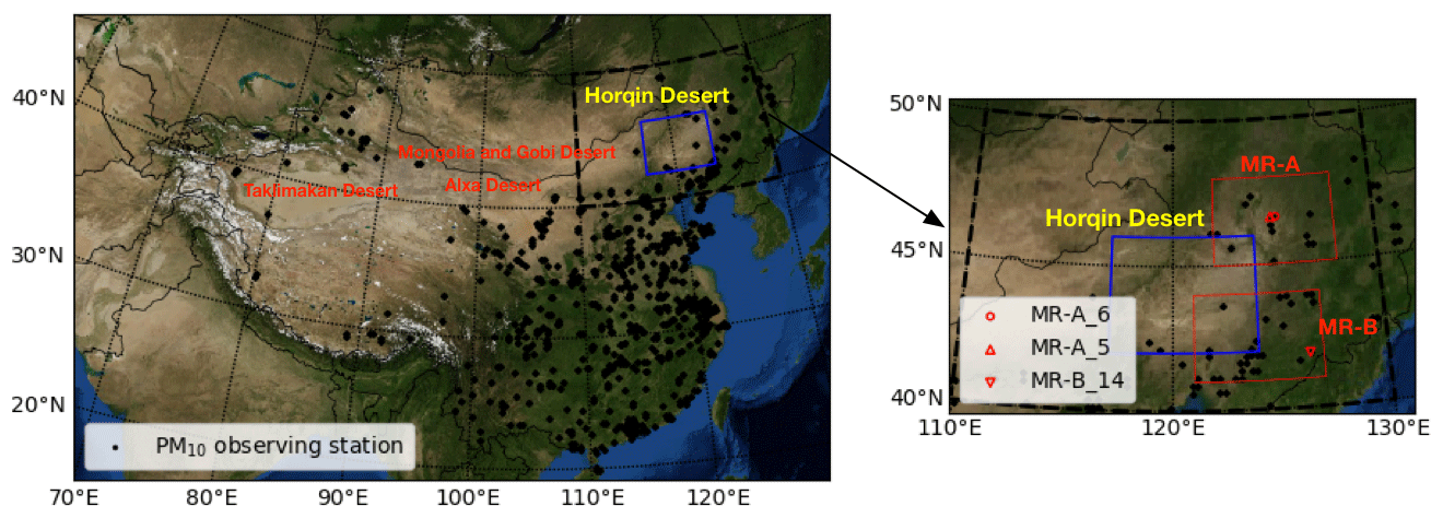
Figure 2 Locations of the Mongolia and Gobi, Alxa, Taklimakan, and Horqin deserts. The dots indicate locations of China MEP air quality monitoring sites. Red marked region A (MR-A) and marked region B (MR-B) are where the dust is observed but not reproduced using the transport model in this study.

Though both the aforementioned Himawari-8 and the ground PM₁₀ data are actually a sum of the dust aerosols and particles released in local activities, the 2017 dust storm events were reported as extremely severe ones, with dust concentrations at downwind cities reaching up to 4000 µg m⁻³; hence, dust aerosols are very dominant in the full aerosols. For such kinds of severe dust events, Mahowald et al. (2017) indicated AOD can be directly used as a reliable tool to represent dust loading in the atmosphere. AODs from Moderate Resolution Imaging Spectroradiometer (MODIS) satellite products and the ground PM₁₀ observations were also directly used to represent dust intensity for the same event in Zhang et al. (2018). Therefore, all these measurements are assumed to be representative for comparison with the dust simulations in this study too. In case of less severe dust storms, observational bias corrections (Dee and Uppala, 2009) would be required to remove the non-dust part from the observations to allow comparison with a “dust-only” model (Jin et al., 2019a). Besides, a variable observation representation error is used in this study to reduce the observation bias influence, as will be explained in Sect. 6.2.

3 Dust model

3.1 Model configuration

A regional chemical transport model, LOTOS-EUROS, is used to simulate the dust lifecycles, including emission, advection, diffusion, dry and wet deposition, and sedimentation (Manders et al., 2017). To simulate dust outbreaks in East Asia, the model is configured on a domain from 15 to 50^∘ N and 70 to 140^∘ E, at a resolution of ${\mathrm{0.25}}^{\circ }\times {\mathrm{0.25}}^{\circ }$. Vertically, the model is configured on eight layers with a top at 10 km, where the second layer is a mixing layer representing a well-mixed boundary layer. The model is driven by meteorological data from the European Centre for Medium-Ranged Weather Forecasts (ECMWF), in this study operational forecasts for horizons of 3–12 h starting from the 00:00 and 12:00 analyses, retrieved at a regular longitude–latitude grid of about 7 km resolution. The dust aerosols in the model are described by five aerosol bins as shown in Table 1.

Table 1 Dust aerosol size distribution in LOTOS-EUROS.

The severe dust storm event studied in this paper took place over East Asia in May 2017 and has already been used as a case study for emission inversion in Jin et al. (2019b). The dust storm first originated from the Gobi and Mongolia deserts and was then carried by the prevailing wind to northern and central China. After crossing northern China, the dust plume moved further east to the Korean Peninsula and Japan (Minamoto et al., 2018), and part of the plume was eventually even transported across the Pacific Ocean (Zhang et al., 2018).

3.2 Dust emission parameterization and error analysis

The physical basis of the dust emission model adopted in LOTOS-EUROS is the parameterization scheme by Marticorena and Bergametti (1995). The dust flux ℱ_v is calculated as a function of horizontal saltation ℱ_h, the sandblasting efficiency α (Shao et al., 1996), a terrain preference 𝒮, and an erodible surface fraction 𝒞 as

$$\begin{array}{}\text{(1)}& {\mathcal{F}}_v={\mathcal{F}}_h\cdot \mathit{\alpha }\cdot \mathcal{S}\cdot \mathcal{C}.\end{array}$$

The dust saltation rate ℱ_h is proportional to the third power of the wind friction velocity u_*, as long as this exceeds a certain (surface-dependent) friction velocity threshold u_*t:

$$\begin{array}{}\text{(2)}& {\mathcal{F}}_h=\left\{\begin{array}{ll}\mathrm{0}& u_{*}\le u_{*t}\\ \frac{p_a}{g}{u}_{*}^{\mathrm{3}}\left(\mathrm{1}+\frac{u_{*t}}{u_{*}}\right)\left(\mathrm{1}-\frac{u_{*t}^{\mathrm{2}}}{u_{*}^{\mathrm{2}}}\right)& u_{*}>u_{*t}\end{array}\right..\end{array}$$

The friction velocity u_* is computed from the ECMWF 10 m wind speed assuming neutral atmospheric stability, following a logarithmic profile. The friction velocity threshold u_*t is derived first for an idealized dry and smooth surface and then increased using two correction factors that described the actual situation in a grid cell: the first factor accounts for soil moisture in the presence of clay and the second factor accounts for surface roughness elements. More formulas and details related to the ℱ_h parameterization can be found in Jin et al. (2018).

Of the other factors in Eq. (1), the sandblasting efficiency α is determined by the average diameter of the soil particles in saltation and the average diameter of suspended particles. The terrain preference 𝒮 represents the probability of having accumulated sediments in a given model cell (Ginoux et al., 2001), calculated as

$$\begin{array}{}\text{(3)}& {\mathcal{S}}_i={\left({\displaystyle \frac{z_{\text{max}}-z_i}{z_{\text{max}}-z_{\text{min}}}}\right)}^{\mathrm{5}},\end{array}$$

where z_i denotes the elevation of the given grid cell i, while z_max and z_min represent the maximum and minimum elevations in the surrounding ${\mathrm{10}}^{\circ }\times {\mathrm{10}}^{\circ }$ area, respectively. Note that a typo error was made in the same terrain preference equation but without a power of 5 in the related PhD thesis (Jin, 2019). The current configuration assumes that only areas that are identified as barren surfaces in the land-use maps allow wind-blown dust emissions, while all vegetated or water-covered surfaces are considered non-erodible. The fraction of barren surface 𝒞 in a grid cell is taken from the Global Land Cover database (http://forobs.jrc.ec.europa.eu/products/glc2000/, last access: April 2020).

Even though the existing parameterizations were already validated with a high credibility either in wind tunnel tests or in simulations for case studies, the representations of these schemes in regional and global atmospheric models are still limited. Many uncertainties are present, for example in the land-use (derived from the Global Land Cover database) and soil databases (derived from the PSU/NCAR mesoscale model known as MM5) that are used as input. These uncertainties result in differences between observations and simulations that cannot be traced back immediately to a single cause. Besides, these deterministic parameterizations are not representative of the stochastic nature of dust emissions. For example, the dust saltation only occurs when u_t exceeds the minimum friction velocity that is needed to initiate a movement of soil particles. However, observations show that within the dust particle size range the threshold friction velocity also differs widely due to stochastic inter-particle cohesion. In reality there will always be a (small) amount of free-moving dust which can be resuspended even by weak wind forces (Shao and Klose, 2016).

Several emission inverse modeling studies have analyzed and estimated sources of dust aerosols on regional scales and decreased uncertainties in the emission model by minimization of observation-minus-simulation differences. However, the large amount of uncertainties cannot be constrained completely by the available observations. Most studies therefore coarsen the uncertainties, limiting the optimization to only a few scaling factors for the emissions field (e.g., Yumimoto et al., 2008) or for precursor emission inputs (e.g., for the relative erodibility surface fraction by Khade et al., 2013, and friction velocity threshold by Di Tomaso et al., 2017, and Jin et al., 2018) spanning large domains. However, a coarse and simplified emission uncertainty configuration might not be able to resolve all observation-minus-simulation differences during the inverse modeling. An example of this will be shown in Sect. 5.2, where three severe dust outbreaks are described. The emission inversion assimilating satellite aerosol optical depth (AOD) was able to produce a posteriori emission fields that lead to dust simulations in agreement with dust observations at ground level, except for a small region in the domain.

4 Adjoint model

The adjoint approach provides an efficient tool for calculating the sensitivity of a simulation model with respect to its input parameters. In this study, an adjoint model is used to identify potential source regions for dust that could explain the mismatch between simulations and observations in the northeast of China.

4.1 Adjoint theory

The following notation will be used for the discrete time step of our simulation model:

$$\begin{array}{}\text{(4)}& {\mathit{x}}^k={\mathcal{M}}^{k-\mathrm{1}}({\mathit{x}}^{k-\mathrm{1}},{\mathit{f}}^{k-\mathrm{1}}).\end{array}$$

In here, x^k denotes the state vector at time k that consists of 3D fields of dust aerosol concentrations for each of the five dust size bins in the model, input vector f^k−1 consists of emission fields for the five size bins, and ℳ^k denotes the model operator that simulates x^k given the state and input at time k−1. For a pure dust transport simulation, the model is linear with respect to both x and f and could therefore be written using matrix operators:

$$\begin{array}{}\text{(5)}& {\mathit{x}}^k={\mathbf{M}}^{k-\mathrm{1}}{\mathit{x}}^{k-\mathrm{1}}+{\mathbf{E}}^{k-\mathrm{1}}{\mathit{f}}^{k-\mathrm{1}}.\end{array}$$

The operator M^k represents the transport part of the model, while E^k represents the emission part. Repeated application of Eq. (5) provides the evolution of the state from time k−K to time k:

$$\begin{array}{}\text{(6)}& {\displaystyle }{\mathit{x}}^k=& {\displaystyle }{\mathbf{M}}^{k-\mathrm{1}}\left({\mathbf{M}}^{k-\mathrm{2}}{\mathit{x}}^{k-\mathrm{2}}+{\mathbf{E}}^{k-\mathrm{2}}{\mathit{f}}^{k-\mathrm{2}}\right)+{\mathbf{E}}^{k-\mathrm{1}}{\mathit{f}}^{k-\mathrm{1}}\text{(7)}& {\displaystyle }=& {\displaystyle }{\mathbf{M}}^{k-\mathrm{1}}\cdot {\mathbf{M}}^{k-\mathrm{2}}{\mathit{x}}^{k-\mathrm{2}}+{\mathbf{M}}^{k-\mathrm{1}}\cdot {\mathbf{E}}^{k-\mathrm{2}}{\mathit{f}}^{k-\mathrm{2}}+{\mathbf{E}}^{k-\mathrm{1}}{\mathit{f}}^{k-\mathrm{1}}\text{(8)}& {\displaystyle }=& {\displaystyle }{\mathbf{M}}^{k-\mathrm{1}}\cdot {\mathbf{M}}^{k-\mathrm{2}}\cdot \mathrm{\dots }\cdot {\mathbf{M}}^{k-(K-\mathrm{1})}\cdot {\mathbf{M}}^{k-K}{\mathit{x}}^{k-K}+\text{(9)}& {\displaystyle }& {\displaystyle }{\mathbf{M}}^{k-\mathrm{1}}\cdot {\mathbf{M}}^{k-\mathrm{2}}\cdot \mathrm{\dots }\cdot {\mathbf{M}}^{k-(K-\mathrm{1})}\cdot {\mathbf{E}}^{k-K}{\mathit{f}}^{k-K}+\text{(10)}& {\displaystyle }& {\displaystyle }\mathrm{\dots }+{\mathbf{M}}^{k-\mathrm{1}}\cdot {\mathbf{E}}^{k-\mathrm{2}}{\mathit{f}}^{k-\mathrm{2}}+{\mathbf{E}}^{k-\mathrm{1}}{\mathit{f}}^{k-\mathrm{1}}.\end{array}$$

We define a model response function as a scalar function of the state:

$$\begin{array}{}\text{(11)}& \mathcal{J}\left({\mathit{x}}^k\right)\in \mathcal{R}.\end{array}$$

The response could for example be defined as the simulation at a single location (an observation site) or an average over multiple grid cells. The gradient of this response function at time k with respect to the input vector f^k−K follows from the application of the chain rule and using the fact that Eq. (9) is the only term in the expansion of x^k that depends on f^k−K:

$$\begin{array}{ll}\text{(12)}& {\displaystyle }{\mathrm{\nabla }}_{{\mathit{f}}^{k-K}}\mathcal{J}\left({\mathit{x}}^k\right)=& {\displaystyle }{\mathrm{\nabla }}_{{\mathit{f}}^{k-K}}{\left({\mathit{x}}^k\right)}^T\cdot {\mathrm{\nabla }}_{{\mathit{x}}^k}\mathcal{J}\left({\mathit{x}}^k\right)\text{(13)}& {\displaystyle }=& {\displaystyle }({\mathbf{E}}^{k-K}{)}^T\cdot ({\mathbf{M}}^{k-K}{)}^T\cdot \mathrm{\dots }\cdot ({\mathbf{M}}^{k-\mathrm{2}}{)}^T{\displaystyle }& {\displaystyle }\cdot ({\mathbf{M}}^{k-\mathrm{1}}{)}^T\cdot {\mathrm{\nabla }}_{{\mathit{x}}^k}\mathcal{J}({\mathit{x}}^k).\end{array}$$

The transpose (M^k)^T of the linear model operator M^k is referred to as the adjoint model. To compute the above gradient ∇𝒥, the adjoint model is applied in a reverse time sequence k−1, k−2, …, k−K. The first adjoint operation in this sequence is applied on the adjoint forcing:

$$\begin{array}{}\text{(14)}& {\mathrm{\nabla }}_{{\mathit{x}}^k}\mathcal{J}\left({\mathit{x}}^k\right).\end{array}$$

An adjoint model is a powerful tool to compute the model response with respect to various input parameters. A useful application is found in 4D variational data assimilation, where it is used to derive the gradient of a cost function for the difference between observations and simulations. In the context of air quality, this approach has been used to constrain initial conditions, emissions, and other uncertain model parameters such as uptake (Elbern et al., 2000; Henze et al., 2009).

For this study, an adjoint implementation of the LOTOS-EUROS model will be used to identify potential emission source regions. The adjoint model is created from the same source code, but using an internal flag it applies adjoint (transpose) versions of the transport and emission operators. Using a negative time step, it is able to run backwards in time, as is required to compute the gradients as in Eq. (12). The assimilation system that is used in this study remains the reduced-tangent-linearization four-dimensional variation (4DVar) that was developed in earlier studies (Jin et al., 2018, 2019a, b), which does not use the adjoint implementation. Although it would be possible to use the adjoint for the assimilation too, it was chosen to keep the assimilation system the same in order to compare results before and after the introduction of new emission sources.

4.2 Testing the implementation of the adjoint model

Before using the adjoint model to identify potential emission sources, the implementation is first illustrated and tested by looking at a single site. A suitable test to validate whether the adjoint model computes the correct sensitivity of the model towards changes in the input is to compare its evaluation with a finite-difference method (Henze et al., 2007a; Guerrette and Henze, 2015). That is, the sensitivity of a model response 𝒥(x^k) to the previous emission field f^k−K is computed either using the adjoint or by perturbing the emission field. For this test, we define the response function as the dust concentration in the grid cell where during the most severe dust plume (SD1) the highest PM₁₀ concentration was observed within marked region MR-A, referred to as “MR-A_6”, the location of which could be found in Fig. 2. The response function becomes

$$\begin{array}{}\text{(15)}& \mathcal{J}\left({\mathit{x}}^k\right)=\mathbf{H}{\mathit{x}}^k,\end{array}$$

where the matrix operator H is actually a row vector with zeros except for the elements that represent the five dust size bins in the selected grid cell:

$$\begin{array}{}\text{(16)}& \mathbf{H}=[\mathrm{0},\mathrm{\dots },\mathrm{0},\mathrm{1},\mathrm{1},\mathrm{1},\mathrm{1},\mathrm{1},\mathrm{0},\mathrm{\dots },\mathrm{0}].\end{array}$$

The adjoint forcing becomes

$$\begin{array}{}\text{(17)}& {\mathrm{\nabla }}_{{\mathit{x}}^k}\mathcal{J}\left({\mathit{x}}^k\right)={\mathbf{H}}^T.\end{array}$$

Time t_k is set to 19:00 on 3 May 2017, when the dust concentration in MR-A_6 peaked.

Following Eq. (12), the sensitivities of this dust concentration towards dust emissions at time t_k−K are

$$\begin{array}{}\text{(18)}& \begin{array}{rl}{\mathrm{\nabla }}_{{\mathit{f}}^{k-K}}\mathcal{J}\left({\mathit{x}}^k\right)=& ({\mathbf{E}}^{k-K}{)}^T\cdot ({\mathbf{M}}^{k-K}{)}^T\cdot \mathrm{\dots }\\ & \cdot ({\mathbf{M}}^{k-\mathrm{2}}{)}^T\cdot ({\mathbf{M}}^{k-\mathrm{1}}{)}^T\cdot {\mathbf{H}}^T.\end{array}\end{array}$$

A snapshot of the adjoint emission sensitivities on 3 May, 13:00 CST is shown in Fig. 3a for one of the five dust size bins in the model. According to these values, the dust concentration in MR-A_6 simulated for 6 h later is most sensitive to emissions that are roughly in the rectangular box. Note that in this example the response function 𝒥 has units of concentrations, which gives ∇_f𝒥 the units of concentrations (µg m⁻³) over emissions (µg m⁻² s⁻¹), equivalent to s m⁻¹.

The same sensitivity could also be calculated using a finite-difference method. For this, 16 locations are chosen within the box shown in Fig. 3a. The locations are marked with dots and put at locations where the adjoint sensitivities are non-zero. Then 16 model runs are performed over [13:00, 19:00], where each run is similar to a standard simulation but using emissions that are only non-zero at [13:00, 14:00] at just 1 of the 16 marked locations. The magnitude of these emissions is simply set to 1 µg m⁻² s⁻¹ for each bin. The result of each simulation is the simulated concentration in µg m⁻³ in the MR-A_6 location at 19:00. The ratio between simulated concentration and emission has units s m⁻¹ and is a measure of the sensitivity of the simulation in MR-A_6 at 19:00 towards an emission at one of the marked locations at 13:00.

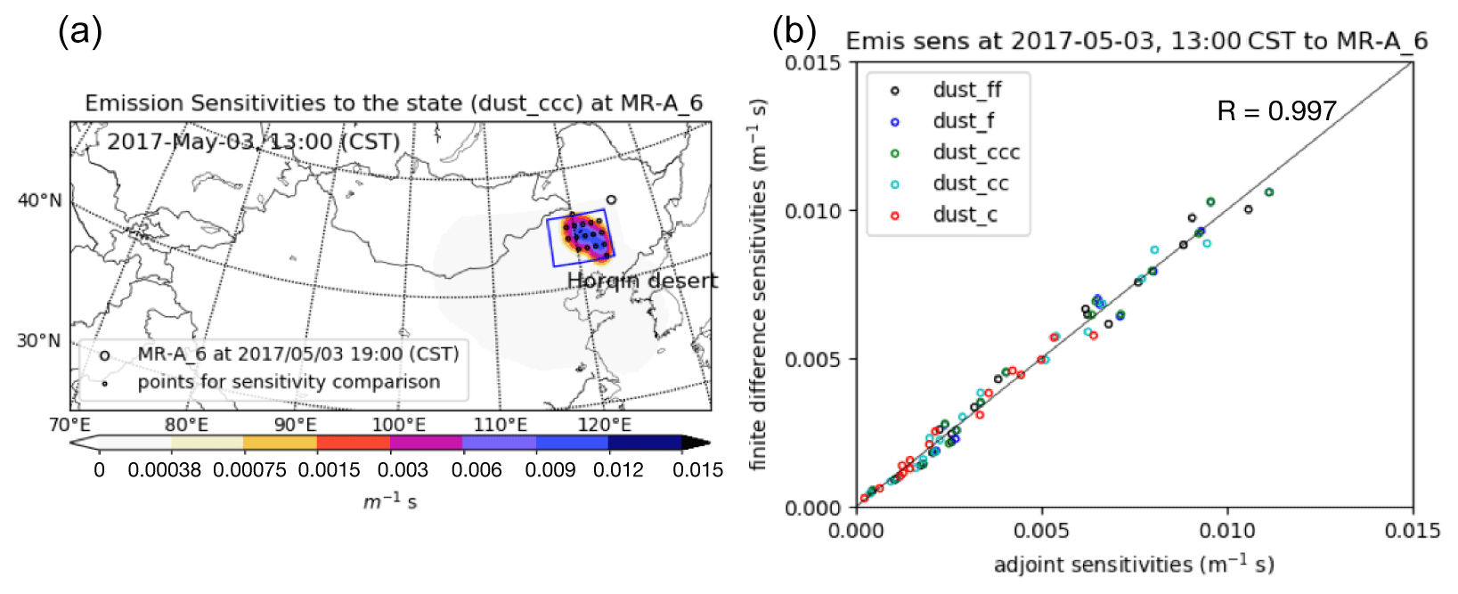
Figure 3 Illustration of sensitivities of dust concentrations at 19:00 in location MR-A_6 towards emissions from selected points at 13:00; (a) map of emission sensitivities computed by the adjoint model; (b) comparison between sensitivities computed by the adjoint method and finite differences.

The scatter plot in Fig. 3b compares the 16 computed sensitivities (for each of the five size bins) versus the sensitivities computed with the adjoint model. The results show that the adjoint-computed sensitivities are in good agreement with the finite-difference sensitivities, which results in a relative high Pearson correlation coefficient of R=0.997. The comparison suggests that the adjoint model has been implemented correctly. The differences that remain might be due to rounding errors at points where the sensitivity is low and model processes other than transport and emission which are not included in the adjoint. Both the finite-difference and adjoint methods seem able to derive emission sensitivities. An advantage of the adjoint method however is that it computes sensitivities with one single simulation, while the finite-difference method requires many more (16 in this example).

5 Dust emission inversion

In Jin et al. (2019b), an assimilation system which combines the same transport model (LOTOS-EUROS) and the reduced-tangent-linearization 4DVar data assimilation (Jin et al., 2018) was used to assimilate from Himawari-8 AOD observations. The assimilation system adjusted the dust emissions in the source regions to obtain the best comparison between simulated and observed AOD. Through comparison with independent PM₁₀ data, the dust concentration forecast was validated to be strongly improved at most downwind sites by the assimilation. However, some large regional simulation errors still remained, especially in Northeast China, as will be discussed later on.

5.1 Dust emission

The uncertainty of the emission in Jin et al. (2019b) was mainly assigned as a sum of two sources, the uncertainty in the friction velocity threshold and in the erosive wind fields. The uncertainty in the friction velocity threshold u_*t was described by a spatially varying multiplicative factor β, defined as random variables with a mean of 1.0 and a standard deviation σ of 10 %. The uncertainty in the friction wind velocity u_* was described by the spread in a meteorological ensemble with 26 members. Note that the dust emission model output data are on every hour per grid cell, and results may vary strongly from hour to hour. Also, dust concentration extremes that last less than 1 h can be missed in model output data. In the inversion system, the temporal variation of the emission model is maintained and could be further increased by the uncertainty during the assimilation window(s) of 24 h.

Figure 4a shows the accumulated dust emission flux from 2 May, 15:00, to 4 May, 15:00 China Standard Time (CST). These dust emissions are responsible for the event that is studied. Outside of this period, the dust emissions are rather weak. The figure shows that the main source regions are in the Gobi and Mongolia deserts. Figure 4b shows the corresponding standard deviation of the accumulated emission that follows from assumed uncertainty.

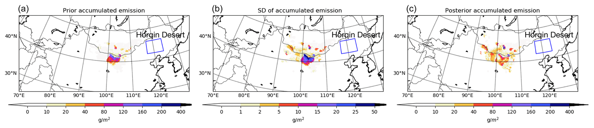
Figure 4 Accumulated prior dust emissions from 2 May 2017, 15:00 (CST) to 4 May, 15:00 (a) as well as the assumed standard deviation (b) and the estimate after assimilation (c). This figure is adapted from Fig. 2 in Jin et al. (2019b).

Two snapshots of Himawari-8 AODs during the tested dust events can be found in Fig. 1. These types of data were assimilated with LOTOS-EUROS simulations in two 24 h windows. The posterior accumulated emissions are also shown in Fig. 4c. Both the prior and posterior simulations indicate that the dust was emitted from the Gobi, Mongolia and Alex deserts. Previous research (Zhang et al., 2018) and simulation from an operational dust forecast model, BSC-DREAM8b (https://ess.bsc.es/bsc-dust-daily-forecast, last access: April 2020), have identified the same emission source for this event.

The red box in Fig. 2 indicates the location of the Horqin desert. The area is not a completely sandy desert but has some vegetation, although sparse. No (or hardly) any dust emissions are assumed to be released from here in the emission model, and therefore the associated uncertainty is also zero. Thus, the Horqin desert is in the model considered completely free of dust emissions, and emissions could also not be introduced by the inversion system. However, as we shall see later on, dust emissions from this region could very well explain observed differences between observations and simulations, and therefore the inversion system should be adjusted to allow emissions from there too.

5.2 Regional differences between observations and posterior simulations

Snapshots of the dust forecasts based on the a posteriori emissions and PM₁₀ concentration during the dust events are shown in Figs. 5 and 6. Although for most locations the a posteriori dust simulations showed good agreement with the PM₁₀ observations, some large mismatches remained, especially in the northeastern part of China. Specifically, extremely high values of surface dust concentration over three severe dust events were reported by the ground-based monitoring system in this region, but neither could be reproduced to the full extent by the simulations. This is illustrated in Fig. 5 for the first severe dust plume from 3 May 2017, 08:00(CST) to 20:00, which we will refer to as “SD1”, and in Fig. 6 for the second dust outbreak from 4 May, 02:00 to 14:00, which is referred to as “SD2”. Similar figures for the third event (“SD3”) are available as the Supplement.

The top row in Fig. 5 shows PM₁₀ observations at three different moments during the SD1 event. Obviously a dust plume crosses the red marked region A (MR-A), with maximum PM₁₀ observations rising rapidly from 200 µg m⁻³ at 08:00 to more than 2000 µg m⁻³ at 20:00. The second and third rows show the a priori and a posteriori LOTOS-EUROS simulations on the surface dust concentration for the same hours. Unfortunately, the simulations in the MR-A region were completely free of dust in both simulations. Note that the simulated prior and posterior AODs, which are not shown here, generally have a similar profile to the surface dust concentration shown in Fig. 5b and c.

The Himawari-8 AOD maps also indicated the existence of a severe dust plume over MR-A, as can be seen in the snapshot of AOD on 3 May, 12:30 in Fig. 1a. Most of the AOD values over MR-A exceed 1.2. Our first 24 h cycle of emission inversion was performed by assimilating these high-valued AOD. The simulations driven by the posterior emission fields, shown in Fig. 5c.1–c.3, did however not lead to a dust load over MR-A during this period. The differences between the posterior simulations and observations indicate that the current emission model and associated uncertainties cannot explain the dust plume in MR-A. In other words, the dust plume that moved over MR-A was not due to emissions from the Gobi and Mongolia deserts we predefined in the background emission but must originate from somewhere else.

The three snapshots of PM₁₀ observations in Fig. 6a indicate the second severe dust plume (SD2) over the same region MR-A. In this case, both prior and posterior LOTOS-EUROS model simulations include a dust plume over MR-A (see Fig. 6b and c), which could be traced back to emissions from the Gobi, Mongolia, and Alex deserts. The maximum of the modeled surface dust concentration over MR-A on 4 May is around 500 µg m⁻³. However, the maximum PM₁₀ measurement value exceeds 2000 µg m⁻³. It is true that these observations minus simulation might be caused by the emission underestimation over the Mongolia and Gobi deserts. Yet those emissions also contributed the dust plume observed in central China. In this case, those dust flux rates are actually constrained at a modest level by those observations. Besides, the dust plume did not fully cover the observed dust-affected regions. Thus, the dust level is considered to be partially due to the predefined emissions but also due to emissions from another region. For this event, Himawari-8 measurements are not successfully retrieved due to cloud scenes over MR-A; thus, AOD snapshots are not available.

The underestimation of dust concentrations over MR-A during the SD1 and SD2 events was also found in other simulation systems, for example, as published by the SDS-WAS service (https://ess.bsc.es/bsc-dust-daily-forecast, last access: April 2020). As an example, results for SD1 and SD2 from the forecast system BSC-DREAM8b (Basart et al., 2012; Mona et al., 2014) are shown in the last row of Figs. 5 and 6, respectively. These suggests that these emission models are also prone to underestimating the emission rate over the Horqin desert.

A similar conclusion was drawn for the third dust outbreak (“SD3”), for which simulation and PM₁₀ measurements are available in the Supplement. For SD3, it was found that a severe dust plume was recorded over the marked region (MR-B) in Northeast China. However, neither the prior nor posterior simulations of the BSC-DREAM8b simulation reproduce any dust over MR-B, although the assimilated Himawari-8 AOD values did indicate the existence of a dust plume over this region, as shown in Fig. 1b.

Figure 5 PM₁₀ observations and surface dust concentrations simulated for the first severe dust event (SD2) for 3 May, 08:00 (CST) (a.1–d.1), 14:00 (a.2–d.2), and 20:00 (a.3–d.3). Top row PM₁₀ observations (a.1–a.3), second row prior simulations (b.1–b.3), third row posterior simulations (c.1–c.3), and bottom row BSC-DREAM8b simulations (d.1–d.3). MR-A: marked region A.

Figure 6 PM₁₀ observations and surface dust concentrations simulated for the second severe dust event (SD2) for 4 May, 02:00 (CST) (a.1–d.1), 08:00 (a.2–d.2), and right column 14:00 (a.3–d.3). Top row PM₁₀ observations (a.1–a.3), second row prior simulations (b.1–b.3), third row posterior simulations (c.1–c.3), and bottom row BSC-DREAM8b simulations (d.1–d.3). MR-A: marked region A.

To further illustrate the three severe dust outbreaks in Northeast China on 3 and 4 May, the time series of the PM₁₀ observations averaged over all monitoring stations inside the marked region MR-A are shown in Fig. 7a. The average PM₁₀ levels are around 100–200 µg m⁻³ when there is no dust (earlier than 2 May, 12:00). The peak of SD1 arrives in marked region MR-A around 3 May 08:00 and has left the region on 4 May 00:00; the averaged PM₁₀ concentrations have reached a value of up to 1000 µg m⁻³. The most severe dust plume occurs during SD2 on 4 May, with average PM₁₀ measurements inside MR-A up to 1500 µg m⁻³.

Figure 7 (a) Hourly PM₁₀ observations averaged over MR-A (13 sites), with shaded area indicating the standard deviation range; (b) root mean square error of prior and posterior simulation, posterior of extra emission inversion, and reconstructed prior and posterior within MR-A. The location of the stations is indicated in Fig. 2.

6 Result and discussion

6.1 Identification of new emission sources

During the investigated severe dust outbreaks (SD1 and SD2), the emission inversion was not able to provide a posteriori simulations that correctly represented the high dust concentrations observed in sites in the northeast of China. To identify whether this could be due to missing dust sources, the adjoint model is used to identify potential source regions.

Similarly to the illustrative example in Sect. 4.2, the sensitivity of a response function towards changes in emissions is computed using the adjoint model for each of the three dust outbreaks. The adjoint forcings H^T in Eq. (18) are chosen as the observed state variables in MR-A_6 on 3 May 19:00 for SD1, in MR-A_5 on 4 May 10:00 for SD2, and in MR-B_14 on 6 May 18:00 for SD3, respectively. The locations of MR-A_6, MR-A_5 and MR-B_14 can be found in Fig. 2b. These three sites (and also the surrounding stations) reported the highest PM₁₀ levels during the three dust outbreaks. For each case, the adjoint forcing H^T is filled with values of 10 µg m⁻³ for each bin in the cell with the observation site. Time series of emission sensitivity fields are shown in Fig. 8 for the severe dust outbreaks SD1 and SD2, while the sensitivities for SD3 are reported in the Supplement.

Figure 8a.1–a.6 show the potential source regions for the high PM₁₀ values observed in MR-A_6 on 3 May, 11:00. The blue marked box encloses the Horqin desert, which is a potential source region for dust emitted 10 h before the observation time. If the dust was emitted earlier, it seems to originate from regions further south, mainly the North China Plain. Though it is also considered a weak potential source by Ginoux et al. (2012), it is a densely populated region covered with vegetation and therefore treated as being further less likely to be a source of dust in our model. Besides, the PM₁₀ observations on 3 May, 03:00 and 06:00 corresponding to the last two snapshots in Fig. 8a are presented in Fig. S3 in the Supplement: they show that the northern China plains were clear of dusts during the event. The sensitivity maps show that for this time period the MR-A_6 location is not sensitive to dust emitted from the Gobi and Mongolia deserts, which are in the current emission model of the main source regions. This explains also why the assimilation system, which was based on adjusting emissions from these deserts, was not able to resolve the high dust levels within marked region MR-A during SD1.

As shown in Fig. 8b.1–b.6, a potential source region for dust observed in marked region MR-A during SD2 is again the Horqin desert, in case the emission took place 12 h before observation. For emissions longer ago, the Gobi and Mongolia deserts could be source regions too. According to the reference and posterior dust simulations in Fig. 6, the dust plume that originated from the Gobi desert was in fact carried to MR-A on 4 May, after 20 to 30 h of long-range transport. However, the simulated dust concentrations in this plume are much lower than the observed PM₁₀ concentrations. The best explanation is that the dust plume was first released from the Gobi desert and that a part of it was carried to Northeast China by the prevailing winds. When it crossed over the Horqin desert, huge amounts of new dust particles were lifted too, and the mixed plume reached marked region MR-A on 4 May. An observational study mainly based on Himawari-8 RGB imagery carried by Minamoto et al. (2018) also indicated that the dust particles in SD2 were not only from the Gobi desert, but might also originate from the Horqin desert, which was up to now recognized as a less active source by most dust emission models.

Similar conclusions were drawn for the severe dust event (“SD3”), for which figures of backward emission sensitivities are available as the Supplement. For SD3, it was noticed that dust emissions from the Horqin desert between 6 May 09:00 and 15:00 could explain the high dust loads observed. Earlier emissions are traced northwards from regions in Siberia or other high-latitude regions as discussed in Bullard et al. (2016) that are still not identified as active source in dust emission models.

The simulation of the emission source sensitivities over the three independent dust events all indicated that the Horqin desert is likely to be the main source region for SD1 and SD3, and also at least partly a source region for SD2. Therefore, the existing emission scheme needs to be adjusted to allow dust emission more erodible from the Horqin desert, especially when dust is observed in Northeast China.

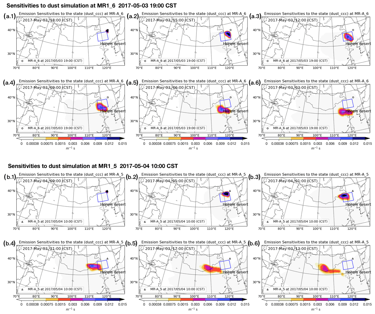
Figure 8 Backward time series of emission sensitivity of the dust simulation at MR-A_6 3 May 2017, 19:00 CST: emission sensitivity distribution on 3 May 2017, 18:00 (a.1), 15:00 (a.2), 12:00 (a.3), 09:00 (a.4), 06:00 (a.5), 03:00 (a.6); and of the dust simulation at MR-A_5 4 May 2017, 10:00: emission sensitivity distribution on 4 May 2017, 09:00 (b.1), 05:00 (b.2), 01:00 (b.3), 3 May, 21:00 (b.4), 17:00 (b.5), 13:00 (b.6).

6.2 Emission inversion with improved emission uncertainty

Parameterization of source areas, which requires knowledge on soil properties and vegetation cover, parameterization of surface roughness, dust emission and transport processes are some possible reasons why the current simulation model is not always able to simulate the actual dust emissions. From the study with the adjoint model it was shown that a lack of emissions from the Horqin desert is likely to be one of these reasons. To allow dust emissions from this region too, the following changes were applied to model the emissions and their uncertainties.

• In the land-use database, most parts of the Horqin desert are described as “sparse vegetated”. For this region, the properties of sparse vegetated surfaces are set similarly to “bare areas”, which leads to a higher erodibility parameter 𝒞_i in Eq. (1).

• The terrain preference correction is disabled, leading to 𝒮_i=1 in Eq. (3).

• A tuning factor 0.7 is used to obtain a lower new friction velocity threshold in Eq. (2).

• The uncertainties in the new emission field is described similarly to Jin et al. (2018, 2019b) by correction factors applied to the new friction velocity threshold. The correction factors are spatially varying and have a mean 1 and a standard deviation 10 %.

These changes are highly empirical and chosen just to have better dust simulations for May 2017. However, these might not be sufficient to correctly describe the emissions from the Horqin dessert during other events. Application in other simulations therefore requires careful inspection by the user.

Table 2 Dust storm emission inversions.

Note: –: no assimilation; emis inver: emission inversion; improved emis: improved emission model.

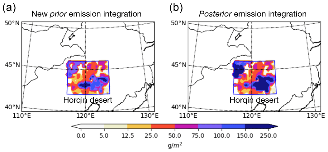
Figure 9 Accumulated dust emissions over the Horqin desert from 3 May, 20:00 CST to 5 May, 07:00 (SD2): (a) prior emissions; (b) posterior emissions. The “old” priori and posterior accumulated emission map can be seen in Fig. 4.

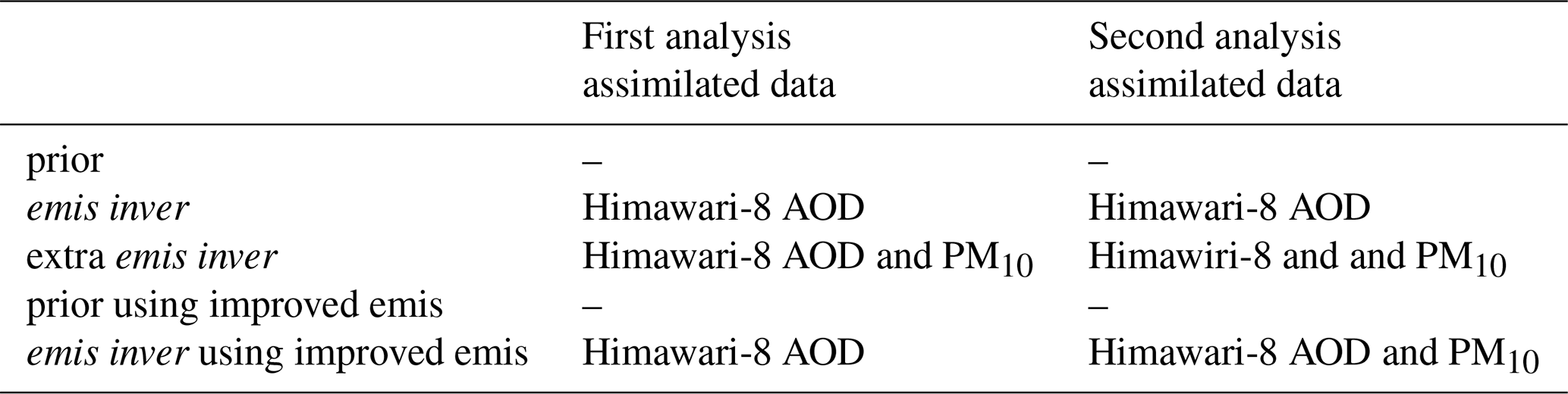
The assimilation of Himawari-8 AODs described in Jin et al. (2019b) The experiment is set from 3 May to 5 May with two 24 h assimilation cycles, which covers the two dust outbreaks, SD1 and SD2, respectively. As seen in Fig. 7b, the two analyses are performed on 4 May, 00:00 and 5 May, 00:00, respectively. Each of them calculates the most likely emission fields in the past 24 h that fits both the prior information and available measurements. Himawari-8 AOD values are assimilated in the first cycle, of which the measurement error configurations are similar to those in Jin et al. (2019b). However, almost no AOD values are retrieved in the second window over the MR-A region; hence, the ground PM₁₀ observations are assimilated additionally. A variable representation error designed in Jin et al. (2018) is used to represent the uncertainty of PM₁₀ measurements, in which a smaller representation error is assigned to measurements reporting a higher PM10 value so that those small-value PM₁₀ observations with larger non-dust fraction will has less influence in assimilation than those high-value measurements. Details over these assimilation tests are listed in Table 2.

The model domain is still configured on the whole of East Asia from 15 to 50^∘ N and 70 to 140^∘ E shown in Fig. 2. The computation complexity on our reduce-tangent-linearization 4DVar is generally proportional to the size of uncertain emission fields. To save the computation costs, the aforementioned new emission and uncertainty are only applied to dust emission over the Horqin desert, while over the rest of the domain, the deterministic emission scheme described in Jin et al. (2019b) is used.

It is actually unfair to compared the results between the emission inversion in Jin et al. (2019b) and the proposed one using improved emission model directly, since the difference could be caused either by extra PM₁₀ observations or by the emission schemes introduced. Therefore, an extra emission inversion is conducted. As shown in Table 2, it repeats the previous emission inversion exactly but extra PM₁₀ observations over the MR-A region are assimilated. The extra emission inversion results in the consistent posterior to the emission inversion in Jin et al. (2019b). The posterior simulation of extra emission inversion is not shown in this paper, but the RMSE time series over MR-A region is calculated and given in Fig. 7b which are approximately the same to the posterior of emission inversion in Jin et al. (2019b). It is because the existing emission background error covariance that explains the emission spread cannot resolve the extra PM₁₀ measurements. The comparison indicates that solely assimilating extra PM₁₀ but without using improved emission modeling has no effect on improving dust emission inversion over Northeast China.

Figure 10 Simulation of SD1 using the new emission fields: (a) a priori and (b) posterior (by assimilating the Himawari-8 AODs) on 3 May, 08:00 (a.1–b.1); 14:00 (a.2–b.2); 20:00 (a.3–b.3). MR-A: marked region A.

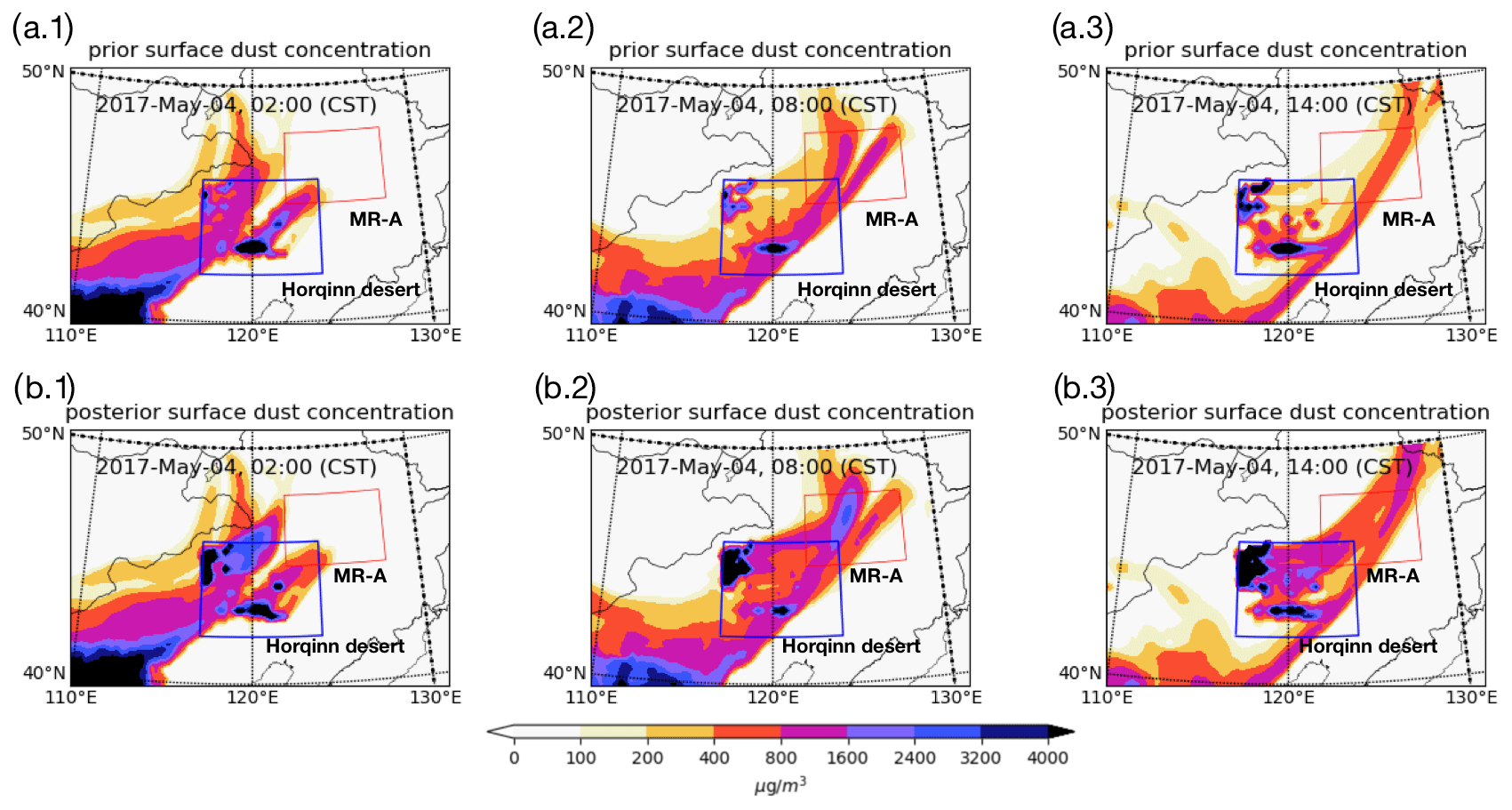
Figure 11 Simulation of SD2 using the new emission fields: (a) prior and (b) posterior (by assimilating the ground-based PM₁₀ observations) on 4 May, 02:00 (a.1–b.1); 08:00 (a.2–b.2); 14:00 (a.3–b.3). MR-A: marked region A.

The emission inversions using the new emission and uncertainty model are then performed. The accumulated dust emissions before and after assimilation are shown in Fig. 9. After assimilation (panel b), a much stronger total emission is estimated than what is computed by the updated a priori model (panel a). In comparison, the “old” parameterization scheme indicates that there is no dust emission at all as shown in Fig. 4. Snapshots of the dust simulations on SD1 and SD2 driven by these emissions are shown in Figs. 10 and 11 for three different times (columns), respectively; in each figure, the top row shows simulations using the reference emissions, and the bottom row using the assimilation result.

These maps could be compared to the observations and simulations using the original emission model as shown in Figs. 5 and 6. Driven by a more easily erodible emission scheme, the a priori simulation (see Fig. 10a) generated a dust band which originated from the Horqin desert and then carried towards the northeast crossing the MR-A. The dust simulation in Fig. 10b are obtained by assimilating the Himawari-8 AOD values on 3 May. This posterior is in better agreement with the real dust load according to the PM₁₀ observations.

During SD2, parts of the dust concentrations in the MR-A originate from a dust plume that was lifted from the Gobi and Mongolia deserts. This initial plume is the result of a LOTOS-EUROS simulation driven by the prior emission scheme. Meanwhile, extra particles are also mobilized from the Horqin desert and transported northwards. The new emission model increases the dust load, however, the simulation without assimilation still under estimates the PM₁₀ concentrations shown in Fig. 6a.1–a.3. Using the posterior emission field, the dust simulations are enhanced further and are in much better agreement with the observations.

To quantify the improvements through the assimilation, the root mean square error (RMSE) between the observed PM₁₀ concentrations and the a priori and posterior dust simulations has been computed for each hour during the two dust outbreaks SD1 and SD2. These RMSE values are added to Fig. 7b, which already showed similar time series for simulations using the original emission model. Using the “new” emission model, the a priori RMSE values are slightly improved compared to the older simulations. Although extra emissions from the Horqin dessert are now included, the default amount is still not strong enough to simulate the observed dust peak, especially during SD2. The largest improvement is made when assimilation is used to further enhance the emissions; the maximum RMSE values during SD1 are reduced from 1100 to 600 µg m⁻³, and during SD2 they are reduced from 2000 to 1000 µg m⁻³. In the original assimilation configuration this could not be achieved since the emission uncertainty model did not allow any additional emissions from the Horqin desert at all.

7 Summary and conclusion

In this study, we illustrate the importance of using a correct background error covariance in emission inversion. An adjoint-based sensitivity method is used to identify new error sources that should be included when constructing emission uncertainties. The methodology is applied to dust outbreaks over East Asia in May 2017.

First, the dust storm emission inversion in Jin et al. (2019b) was reviewed. Although in there improvements in dust simulations and forecasts have been achieved through assimilation of Himawari-8 satellite AOD, large errors still remained unresolved at some locations. Specifically, three severe dust outbreaks in Northeast China were investigated, which are neither reproduced by the a priori nor posterior simulation despite the assimilated measurements indicating the existence of severe dust plumes.

To trace back the potential emission sources, an adjoint model has been introduced, which efficiently calculates the sensitivities of model responses with respect to a large number of input parameters. Evaluation showed that the adjoint sensitivities are in good agreement with the values obtained using a finite-difference method. The adjoint model was then used to trace the sensitivity of three independent dust events to emissions from upwind regions. All the experiments indicate that the Horqin desert is the most likely source region, which is modeled as a non-source in our existing emission parameterizations.

The emission scheme and the corresponding uncertainties over the Horqin desert are then reconstructed by assigning higher erodibility. The agreement with observations is only slightly improved when using a standard model simulation. However, more significant improvements are made when a new assimilation is carried out that is able to further enhance the new emissions. The maximum RMSE between dust simulation and PM₁₀ observations are reduced from 2000 to 1100 µg m⁻³. In future, the residues could be further reduced using a better reference emission as well as an improved uncertainty description for the Horqin desert. Note that also the presence of non-dust particles in the PM₁₀ observations limits the assimilation accuracy; removal of the non-dust part as in (Jin et al., 2019a) will become part of the standard procedure in the future work when the huge amount of computing power is available.

Although existing emission scheme work properly for most deserts in East Asia, e.g., Gobi and Mongolia, they seem to highly underestimate the Horqin desert as a source region. Based on our results, it is advised that dust sources in dust transport models include the Horqin desert as a more active source region, especially when severe dust is observed in Northeast China.

Our study clearly shows the importance of using a correct background error covariance in resolving observation-minus-simulation errors in emission inversions. The proposed adjoint method could also be performed to identify the sensitivity towards emission sources and guide the construction of emission uncertainties. This does not only hold for applications focusing on dust, but also for other atmospheric inverse modeling applications, e.g., black carbon, haze, or gases in case that their source locations are not fully known yet.