the Creative Commons Attribution 4.0 License.
the Creative Commons Attribution 4.0 License.
 | 07 Dec 2020
Methane mapping, emission quantification, and attribution in two European cities: Utrecht (NL) and Hamburg (DE)
Julianne M. Fernandez
Malika Menoud
Daniel Zavala-Araiza
Zachary D. Weller
Stefan Schwietzke
Joseph C. von Fischer
Hugo Denier van der Gon
Thomas Röckmann
Characterizing and attributing methane (CH4) emissions across varying scales are important from environmental, safety, and economic perspectives and are essential for designing and evaluating effective mitigation strategies. Mobile real-time measurements of CH4 in ambient air offer a fast and effective method to identify and quantify local CH4 emissions in urban areas. We carried out extensive campaigns to measure CH4 mole fractions at the street level in Utrecht, the Netherlands (2018 and 2019), and Hamburg, Germany (2018). We detected 145 leak indications (LIs; i.e., CH4 enhancements of more than 10 % above background levels) in Hamburg and 81 LIs in Utrecht. Measurements of the ethane-to-methane ratio (C2:C1), methane-to-carbon dioxide ratio (CH4:CO2), and CH4 isotope composition (δ13C and δD) show that in Hamburg about 1∕3 of the LIs, and in Utrecht 2∕3 of the LIs (based on a limited set of C2:C1 measurements), were of fossil fuel origin. We find that in both cities the largest emission rates in the identified LI distribution are from fossil fuel sources. In Hamburg, the lower emission rates in the identified LI distribution are often associated with biogenic characteristics or (partly) combustion. Extrapolation of detected LI rates along the roads driven to the gas distribution pipes in the entire road network yields total emissions from sources that can be quantified in the street-level surveys of 440±70 t yr−1 from all sources in Hamburg and 150±50 t yr−1 for Utrecht. In Hamburg, C2:C1, CH4:CO2, and isotope-based source attributions show that 50 %–80 % of all emissions originate from the natural gas distribution network; in Utrecht more limited attribution indicates that 70 %–90 % of the emissions are of fossil origin. Our results confirm previous observations that a few large LIs, creating a heavy tail, are responsible for a significant proportion of fossil CH4 emissions. In Utrecht, 1∕3 of total emissions originated from one LI and in Hamburg from two LIs. The largest leaks were located and fixed quickly by GasNetz Hamburg once the LIs were shared, but 80 % of the (smaller) LIs attributed to the fossil category could not be detected and/or confirmed as pipeline leaks. This issue requires further investigation.
- Article
(17165 KB) - Full-text XML
-
Supplement
(8871 KB) - BibTeX
- EndNote


Methane (CH4) is the second most important anthropogenic greenhouse gas (GHG) after carbon dioxide (CO2) with a global warming potential of 84 compared to CO2 over a 20-year time horizon (Myhre et al., 2013). The increase in CH4 mole fraction from about 0.7 ppm (parts per million) or 700 ppb (parts per billion) in pre-industrial times (Etheridge et al., 1998; MacFarling Meure et al., 2006) to almost 1.8 ppm at present (Turner et al., 2019) is responsible for about 0.5 W m−2 of the total 2.4 W m−2 radiative forcing since 1750 (Etminan et al., 2016; Myhre et al., 2013). In addition to its direct radiative effect, CH4 plays an important role in tropospheric chemistry and affects the mixing ratio of other atmospheric compounds, including direct and indirect greenhouse gases, via reaction with the hydroxyl radical (OH), the main loss process of CH4 (Schmidt and Shindell, 2003). In the stratosphere CH4 is the main source of water vapor (H2O) (Noël et al., 2018), which adds another aspect to its radiative forcing. Via these interactions the radiative impact of CH4 is actually higher than what can be ascribed to its mixing ratio increase alone, and the total radiative forcing ascribed to emissions of CH4 is estimated to be almost 1 W m−2, ≈60 % of that of CO2 (Fig. 8.17 in Myhre et al., 2013). Given this strong radiative effect and its relatively short atmospheric lifetime of about 9.1±0.9 yr (Prather et al., 2012), CH4 is an attractive target for short- and medium-term mitigation of global climate change as mitigation will yield a rapid reduction in warming rates.
CH4 emissions originate from a wide variety of natural and anthropogenic sources; this includes, for example, emissions from natural wetlands, agriculture (e.g., ruminants or rice agriculture), and waste decomposition, as well as emissions (intended and non-intended) from oil and gas activities that are associated with production, transport, processing, distribution, and end use in the fossil fuel sector (Heilig, 1994). Fugitive unintended and operation-related emissions occur across the entire oil and natural gas supply chain. In the past decade, numerous large studies have provided better estimates of the emissions from extended oil and gas production basins (Allen et al., 2013; Karion et al., 2013; Omara et al., 2016; Zavala-Araiza et al., 2015; Lyon et al., 2015), the gathering and processing phase (Mitchell et al., 2015), and transmission and storage (Zimmerle et al., 2015; Lyon et al., 2016) in the United States (US). A recent synthesis concludes that the national emission inventory of the US Environmental Protection Agency (EPA) underestimated supply chain emissions by as much as 60 % (Alvarez et al., 2018). McKain et al. (2015) discussed how inventories may underestimate the total CH4 emission for cities. Also, an analysis of global isotopic composition data suggests that fossil-related emissions may be 60 % higher than what has been previously estimated (Schwietzke et al., 2016). A strong underestimate of fossil-fuel-related emissions of CH4 was also implied by an analysis of δ14C–CH4 in pre-industrial air (Hmiel et al., 2020). These emissions do not only have adverse effects on climate, but also represent an economic loss (Xu and Jiang, 2017) and a potential safety hazard (West et al., 2006). While CH4 is the main component in natural gas distribution networks (NGDNs), composition of natural gas varies from one country or region to another. In Europe the national authorities provide specifications on components of natural gas in the distribution network (Table 8 in UNI MISKOLC and ETE, 2008).
Regarding CH4 emissions from NGDNs, a number of intensive CH4 surveys with novel mobile high-precision laser-based gas analyzers in US cities have recently revealed the widespread presence of leak indications (LIs: CH4 enhancements of more than 10 % above background level) with a wide range of magnitudes (Weller et al., 2018, 2020; von Fischer et al., 2017; Chamberlain et al., 2016; Hopkins et al., 2016; Jackson et al., 2014; Phillips et al., 2013). The number and severity of natural gas leaks appear to depend on pipeline material and age, local environmental conditions, and pipeline maintenance and replacement programs (von Fischer et al., 2017; Gallagher et al., 2015; Hendrick et al., 2016). For example, NGDNs in older cities with a larger fraction of cast iron or bare steel pipes showed more frequent leaks than NGDNs that use newer plastic pipes. The data on CH4 leak indications from distribution systems in cities are valuable for emission reduction in US cities, which allows local distribution companies (LDCs) in charge of NGDNs to quickly fix leaks and allocate resources efficiently (Weller et al., 2018; von Fischer et al., 2017; Lamb et al., 2016; McKain et al., 2015).
The CH4 emissions in urban European cities are not well known, which requires carrying out extensive campaigns to collect required observation data. Few studies have estimated urban CH4 fluxes using eddy covariance measurements (Gioli et al., 2012; Helfter et al., 2016), airborne mass balance approaches (O'Shea et al., 2014), and the radon-222 flux and mixing layer height techniques (Zimnoch et al., 2019). Gioli et al. (2012) showed that about 85 % of methane emissions in Florence, Italy, originated from natural gas leaks. Helfter et al. (2016) estimated CH4 emissions of 72±3 t km−2 yr−1 in London, UK, mainly from sewer system and NGDN leaks, which is twice as much as reported in the London Atmospheric Emissions Inventory. O'Shea et al. (2014) also showed that CH4 emissions in greater London are about 3.4 times larger than the report from the UK National Atmospheric Emission Inventory. Zimnoch et al. (2019) estimated CH4 emissions of m3 yr−1 for Kraków, Poland, based on data for the period of 2005 to 2008 and concluded that leaks from NGDNs are the main emission source in Kraków based on the carbon isotopic signature of CH4. Chen et al. (2020) also showed that incomplete combustion or loss from temporarily installed natural gas appliances during big festivals can be the main source of CH4 emissions from such events, while these emissions have not been included in inventory reports for urban emissions.
Here we present the results of mobile in situ measurements at the street level for whole-city surveys in two European cities, Utrecht in the Netherlands (NL) and Hamburg in Germany (DE). In this study, we quantified LI emissions using an empirical equation from Weller et al. (2019), which was designed based on controlled release experiments from von Fischer et al. (2017), to quantify ground-level emission locations in urban area, such as leaks from NGDNs. In addition to finding and categorizing the CH4 enhancements (in a similar manner as done for the US cities in order to facilitate comparability), we made three additional measurements to better facilitate source attribution: the concomitant emission of ethane (C2H6) and CO2 and the carbon and hydrogen isotopic composition of the CH4. These tracers allow an empirically based source attribution for LIs. In addition to emission quantifications of LIs across the urban areas in these two cities, we also quantified CH4 emissions from some of the facilities within the municipal boundary of Utrecht and Hamburg using a Gaussian plume dispersion model (GPDM).
2.1 Data collection and instrumentation
2.1.1 Mobile measurements for attribution and quantification
Mobile atmospheric measurements at the street level were conducted using two cavity ring-down spectroscopy (CRDS) analyzers (Picarro Inc. model G2301 and G4302), which were installed on the back seat of a 2012 Volkswagen Transporter (see Sect. S1.1 and Fig. S1 in the Supplement). The model G2301 instrument provides atmospheric mole fraction measurements of CO2, CH4, and H2O, each of them with an integration time of about 1 s, which results in a data frequency of ≈0.3 Hz for each species. The reproducibility for CH4 measurements was ≈1 ppb for 1 s integration time. The G2301 instrument was powered by a 12 V car battery via a DC-to-AC converter. The flow rate was ≈187 mL min−1. Given the volume and pressure of the measurement cell (volume 50 mL and pressure ≈190 mbar) the cell is flushed approximately every 3 s, so observed enhancements are considerably smoothed out. The factory settings for CH4 and CO2 were used for the water correction.
The G4302 instrument is a mobile analyzer that provides atmospheric mole fraction measurements of C2H6, CH4, and H2O. The flow rate is 2.2 L min−1 and the volume of the cell is 35 mL (operated at 600 mb, thus 21 mL at standard temperature and pressure – STP) so the cell is flushed in 0.01 s, which means that mixing is insignificant given the 1 s measurement frequency of the G4302. The additional measurement of C2H6 is useful for source attribution since natural gas almost always contains a significant fraction of C2H6, whereas microbial sources generally do not emit C2H6 (Yacovitch et al., 2014). The G4302 runs on a built-in battery that lasts for ≈6 h. The instrument can be operated in two modes at ≈1 Hz frequency for each species: the CH4-only mode and the CH4–C2H6 mode. In the CH4-only mode the instrument has a reproducibility of ≈10 ppb for CH4. The factory settings for CH4 and C2H6 were used for the water correction. In the CH4–C2H6 mode the reproducibility is about 100 ppb for CH4 and 15 ppb for C2H6. For Utrecht surveys (see Sect. S1.2, Fig. S2a), the G4302 was not yet available for the initial surveys in 2018, but it was added for the later revisits (see Sect. S1.2, Table S1 in the Supplement). For Hamburg (see Sect. S1.2, Fig. S2b), both instruments operated during the entire intensive 3-week measurement campaign in October–November 2018 (see Sect. S1.2, Table S2). The time delay from the inlet to the instruments was measured and accounted for in the data processing procedure. The Coordinated Universal Time (UTC) time shifts between the Global Positioning System (GPS) and the two Picarro instruments were corrected for each instrument in addition to the inlet delay (see Sect. S1.2, Tables S1 and S2). The clocks on the Picarro instruments were set to UTC but showed drift over the period of the campaigns. We recorded the drifts for each day's survey and corrected to UTC. The data were also corrected for the delay between air at the inlet and the signal in the CH4 analyzers. This delay was determined by exposing the inlet to three small CH4 pulses from exhaled breath, ranging from 5–30 s, depending on the instrument and tubing length. We averaged the three attempts to determine the delay for each instrument and used the delays for each instrument. Individual attempts were 1 to 2 s different from each other. For the G4302 the delay was generally about 5 s and for the G2301 it was about 30 s; the difference is mainly due to the different flow rates. The recorded CH4 mole fractions were projected back along the driving track according to this delay.
Teflon tubing (0.25 in.) was used to pull in air either from the front bumper (0.5 m a.g.l. – above ground level) to the G2301 or from the rooftop (2 m a.g.l.) to the G4302. To avoid dust in the inlets for both instruments, and Acrodisc® syringe filter (0.2 µm) was used for G2301 and Parker Balston 9933-05-DQ was used for G4302. The G2301 was used for quantification and attribution purposes and the G4302 mainly for attribution. After a data quality check, a comparison between the two instruments during simultaneous measurements showed that all LIs were detectable by both instruments despite the difference in instrument characteristics and inlet height (see Sect. S1.3, Fig. S3). In the majority of cases CH4 enhancements for each LI from both instruments were similar to each other. We note that there is likely a compensation of differences from two opposing effects between the two measurement systems. The inlet of the G2301 was at the bumper and thus closer to the surface sources, but the rather low flow rate and measurement rate of the instrument led to some smoothing of the signal in the cavity. Because of the high gas flow rate, signal smoothing is greatly reduced for the G4302, but the inlet was on top of the car and thus further away from the surface sources (see Table S3, Sect. S1.3). The vehicle locations were registered using a GPS that recorded the precise driving track during each survey.
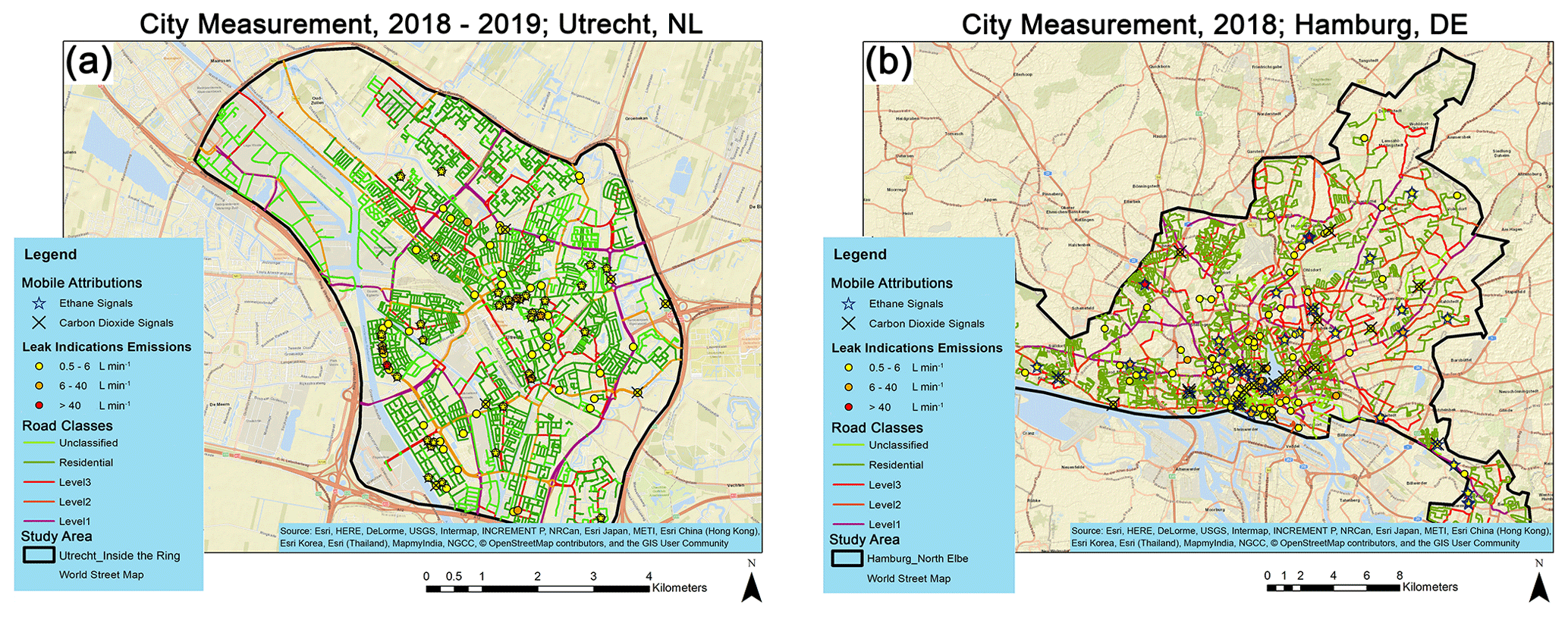
Figure 1Locations of significant LIs for the categories on different street classes in (a) Utrecht and (b) Hamburg. Road colors indicate the street classes according to the OSM. Black polygons show urban study areas.
2.1.2 Target cities: Utrecht and Hamburg
Utrecht is the fourth largest city in the Netherlands with a population of approximately 0.35 million within an area of roughly 100 km2. It is located close to the center of the Netherlands and is an important infrastructural hub in the country. The Utrecht city area that we target in this study is well constrained by a ring of highways around the city (A27, A12, A2, and N230) with approximately 0.28 million inhabitants living within this ring on roughly 45 km2 of land. Figure S2a (see Sect. S1.2) shows the streets that were driven in Utrecht and Fig. 1a shows the street coverage over four street categories (level 1, 2, 3, residential, and unclassified) obtained from the Open Street Map (OSM; https://www.openstreetmap.org/#map=6/51.330/10.453, last access: 22 April 2019). Table S4 (see Sect. S1.5) provides information on road coverage based on different street categories. The hierarchy of OSM road classes is based on the importance of roads in connecting parts of the national infrastructure. Level 1 roads are primarily larger roads connecting cities, level 2 roads are the second most important roads and part of a greater network to connect smaller towns, and level 3 roads have tertiary importance and connect smaller settlements and districts. Residential roads are roads that connect houses, and unclassified roads have the lowest importance of interconnecting infrastructure. Moreover, several transects were also made to measure the atmospheric mole fraction of CH4 from the road next to the waste water treatment plant (WWTP) in Utrecht – a potentially larger single source of CH4 emissions in the city (see Sect. S1.6, Table S5).
Hamburg is the second largest city in Germany (about 1.9 million inhabitants, 760 km2 area) and hosts one of the largest harbors in Europe. The study area in Hamburg is north of the Elbe river (Fig. 1b) with ≈1.4 million inhabitants on about 400 km2 land. Figure S2b (see Sect. S1.2) shows the streets that were covered in Hamburg and Fig. 1b shows the street coverage categorized in the four categories of OSM. More information on road coverage based on OSM street categories is provided in Table S4 (see Sect. S1.5). The local distribution companies (LDCs) in Utrecht (STEDIN; https://www.stedin.net/, last access: 30 September 2020) and Hamburg (GasNetz Hamburg; https://www.gasnetz-hamburg.de, last access: 20 October 2020) confirmed that full pipeline coverage is available beneath all streets. Therefore, the length of roads in the study areas of Utrecht and Hamburg are representative of NGDN length. The Hamburg harbor area hosts several large industrial facilities that are related to the midstream and downstream oil and gas sector, including refineries and storage tanks. An oil production site (oil well, separator, and storage tanks) at Allermöhe (in Hamburg-Bergedorf) was also visited. Information from the State Authority for Mining, Energy and Geology (LBEG, 2018) was used to locate facilities. Precise locations of the facilities surveyed are given in the Table S6 (see Sect. S1.6). In order to separate these industrial activities from the NGDN emissions in this study, CH4 emissions from these locations were estimated, but evaluated apart from the emissions found in each city. The reported in situ measurements, GPS data, and boundaries of study areas reported here are available on the Integrated Carbon Observation System (ICOS) portal (Maazallahi et al., 2020b).
2.1.3 Driving strategy
The start and end points for each day's measurement surveys across Utrecht and Hamburg were the Institute for Marine and Atmospheric research Utrecht (IMAU; Utrecht University) and the Meteorological Institute (MI; Hamburg University), respectively. From these starting locations, each day's surveys targeted the different districts and neighborhoods of the cities (see Sect. S1.2, Tables S1 and S2). Measurement time periods and survey areas were chosen to select favorable traffic and weather conditions and to avoid large events (e.g., construction; see Sect. S1.5, Fig. S4), which normally took place between 10:00 and 18:00 LT. Average driving speeds on city streets were in the range of 17±7 km h−1 in Utrecht and 20±6 km h−1 in Hamburg.
As part of our driving strategy, we revisited locations where we had observed enhanced CH4 readings (see Sect. S1.7, Fig. S5). Not all recorded CH4 mole fraction enhancements are necessarily the result of a stationary CH4 source. For example, they could be related to emissions from vehicles that run on compressed natural gas or vehicles operated with traditional fuels but with faulty catalytic converter systems. Later we will discuss how to exclude or categorize these unintended signals (see Sect. 2.2.2 and 2.3.1). Therefore, we revisited a large number of locations – 65 in Utrecht (≈80 %) and 100 in Hamburg (≈70 % – where enhanced CH4 had been observed during the first survey in order to confirm the LIs. In contrast to the measurements carried out in many cities in the United States (US) (von Fischer et al., 2017), our measurements were not carried out using Google Street View cars, but with a vehicle from the Institute for Marine and Atmospheric research Utrecht (IMAU), Utrecht University (see Sect. S1.1, Fig. S1). Due to time and budget restrictions, it was not possible to cover each street at least twice, as done for the US cities. After evaluation of the untargeted first surveys that covered each street at least once, targeted surveys were carried out for verification of observed LIs and for collection of air samples at locations with high CH4 enhancements. The rationale behind this measurement strategy is that if an enhancement was not recorded during the first survey, it obviously cannot be verified in the second survey. The implications of the difference in the measurement strategy will be discussed in the Results and Discussion sections below.
In total, approximately 1300 km of roads were driven during Utrecht surveys and about 2500 km during the Hamburg campaign. In Utrecht, some revisits were carried out several months to a year after the initial surveys in order to check the persistence of the LIs. In Hamburg, revisits were also performed within the 4-week intensive measurement period. Further details about the driving logistics are provided in Sect. S1.6 and Tables S1 and S2. It is possible that pipeline leaks that were detected during the initial survey were repaired before the revisit, and the chance of this occurring increases as the time interval between visits gets longer.
2.1.4 Air sample collection for attribution
In addition to the mobile measurement of C2H6 and CO2 for LI attribution purposes, samples for lab isotope analysis of δ13C–CH4 and δ2H–CH4 (hereinafter δ13C and δD, respectively) were collected during the revisits at locations that had displayed high CH4 enhancements during the first surveys. Depending on the accessibility and traffic, samples were either taken inside the car (see Sect. S1.8, Fig. S6a) using tubing from the bumper inlet or outside the car on foot using the readings from the G4302 to find the best location within the plume (see Sect. S1.8, Fig. S6b). All the samples taken in the north Elbe study area and from most of the facilities were collected when the car was parked, but the samples inside the new Elbe tunnel and close to some facilities where there was no possibility to park were taken in motion while we were within the plume. The sampling locations across the north Elbe study area in Hamburg were determined based on the untargeted surveys and the confirmation during revisits. The C2H6 information was not used in the selection of sampling locations in order to avoid biased sampling. Sampling locations from the facilities were determined based on wind direction, traffic, and types of activities. Samples for isotope analysis were collected in non-transparent aluminum-coated Tedlar Supelco SeupelTM Inert SCV gas sampling bags (2 L) and SKC standard FlexFoil® air sample bags (3 L) using a 12 V pump and 1∕4 in. Teflon tubing that pumps air with a flow rate of ≈0.25 L min−1. In total, 103 bag samples were collected at 24 locations in Hamburg, 14 of them in the city area north of the Elbe river and 10 at larger facilities. Usually, three individual samples were collected at each source location, plus several background air samples on each sampling day. This sampling scheme generally results in a range of mole fractions that allow source identification using a Keeling plot analysis (Keeling, 1958, 1961). Fossil CH4 sources in the study areas for this paper (inside the ring for Utrecht and north Elbe in Hamburg) refer to emissions originating from natural gas leaks.
2.1.5 Meteorological data
Meteorological information reflecting the large-scale wind conditions during the campaigns was obtained from measurements at the Cabauw tower (51.970263∘ N, 4.926267∘ E) operated by the Koninklijk Nederlands Meteorologisch Instituut (KNMI) (Van Ulden and Wieringa, 1996) for Utrecht and the Billwerder tower (53.5192∘ N, 10.1029∘ E) operated by the MI at Hamburg University (Brümmer et al., 2012) for Hamburg. The wind direction and wind speed data from the masts were used for planning the surveys. Pressure and temperature measurements were used to convert volume to mass fluxes for CH4. We also used information from the towers for the GPDM calculations of the emission rates from larger facilities because the local wind measurements from the 2-D anemometer were not logged continuously due to failure in logging the setup of the measurements. In Utrecht, the Cabauw tower is located about 20 km from the WWTP. In Hamburg the Billwerder tower is about 18 km from the soil and compost company and about 8 km from oil production facilities. Uncertainties in the wind data will be described later.
2.2 Emission quantification
2.2.1 Data preparation and background extraction of mobile measurements
The first step of the evaluation procedure is quality control of the data from both CH4 analyzers and the GPS records. Periods of instrument malfunction and unintended signals based on notes written during each day's measurements were removed from the raw data. Extraction of the LIs from in situ measurements requires estimation of the background levels (see Sect. S2.1, Fig. S7). We estimated the CH4 background as the median value of ±2.5 min of measurements around each individual point as suggested in Weller et al. (2019). For estimating the CO2 background level we used the 5th percentile of ±2.5 min of measurements around each individual point (Brantley et al., 2014; Bukowiecki et al., 2002). The background determination method for CH4 was selected from Weller et al. (2019) to follow the emission quantification algorithm for urban studies, and while this algorithm does not include background extraction for CO2, we chose the commonly adopted method of background determination for this component. These background signals were subtracted from the measurement time series to calculate the CH4 and CO2 enhancements. For C2H6, the background was considered zero as it is normally present at a very low mole fraction between ∼0.4 and 2.5 ppb (Helmig et al., 2016) and is lower than the G4302 detection limit.
2.2.2 Quantification of methane emissions from leak indications
We wrote an automated MATLAB® script (available on GitHub from Maazallahi et al., 2020a) based on the approach initially introduced in von Fischer et al. (2017) and improved in Weller et al. (2019). This algorithm was designed to quantify CH4 emissions from ground-level emission release locations within 5–40 m from the measurement (von Fischer et al., 2017), such as pipeline leaks, and it has been demonstrated that the algorithm adequately estimates the majority of those emissions from a city (Weller et al., 2018). Using the same algorithm also ensures that results are comparable between European and US cities. The individual steps will be described below. Mapping and spatial analysis were conducted using Google Earth and ESRI ArcMap software. A flow diagram of the evaluation procedure is provided in Sect. S2.2 and Fig. S8.
Following the algorithm from von Fischer et al. (2017), measurements at speeds above 70 km h−1 were excluded, as the data from the controlled release experiments (von Fischer et al., 2017) were not reliable at high speed (Weller et al., 2019). We also excluded measurements during periods of zero speed (stationary vehicle) to avoid unintended signals coming from other cars running on compressed natural gas when the measurement car was stopped in traffic. In order to merge the sharp 1 Hz-frequency records of the GPS with the ≈0.3 Hz data from the G2301 analyzer, the CH4 mole fractions were linearly interpolated to the GPS times.
Weller et al. (2019) established an empirical equation to convert LIs observed with a Picarro G2301 in a moving vehicle in urban environments into emission rates based on a large number of controlled release experiments in various environments (Eq. 1).
In this equation, C represents CH4 enhancements above the background in parts per million (ppm) and Q is the emission rate in liters per minute (L min−1). Weller et al. (2019) used controlled releases to demonstrate that the magnitude of the observed methane enhancement is related to the emission rate and carefully characterized the limitations and associated errors of this equation. We used Eq. (1) to convert CH4 enhancements encountered during our measurements in Utrecht and Hamburg to emission rates, and we use these estimates to categorize LIs into three classes: high (emission rate > 40 L min−1), medium (emission rate 6–40 L min−1), and low (emission rate 0.5–6 L min−1), following the categories from von Fischer et al. (2017) (Table 1).
Table 1Natural gas distribution network CH4 emission categories.

The spatial extent of individual LIs was estimated as the distance between the location where the CH4 mole fraction exceeded the background by more than 10 % (≈0.200 ppm; as used in von Fischer et al., 2017, and Weller et al., 2019) and the location where it fell below this threshold level again. LIs that stay above the threshold for more than 160 m were excluded in the automated evaluation because we suspect that such extended enhancements are most likely not related to leaks from the NGDN (von Fischer et al., 2017).
In a continuous measurement survey on a single day, consecutive CH4 enhancements above background observed within 5 s were aggregated and the location of the emission source was estimated based on the weighted averaging of coordinates (Eq. 2). Decimal degree coordinates were converted to Cartesian coordinates (see Sect. S2.3, Fig. S9) relative to local references (see Sect. S2.3, Table S7). In Utrecht, the Cathedral tower (Domtoren) and in Hamburg St. Nicholas' Church were selected as local geographic datums. LIs observed on different days at similar locations were clustered and interpreted as one point source when circles with a 30 m radius around the center locations overlapped, similar to Weller et al. (2019). The enhancement of the cluster was assigned the maximum observed mole fraction and located as the weighted average of the geographical coordinates of the LIs within that cluster (Eq. (2) from Weller et al., 2019), where wi is the CH4 enhancement of each LI.
We compared the outputs of our software to the one developed by Colorado State University (CSU) for the surveys in US cities (von Fischer et al., 2017; Weller et al., 2019). A total of 30 LIs were detected and no significant differences were observed (linear fit equation , R2=0.99) (see Sect. S2.4, Fig. S10). As mentioned above, in our campaign-type studies not all streets were visited twice, so this criterion was dropped from the CSU algorithm. Instead, we used explicit source attribution by co-emitted tracers.
The emission rate per kilometer of road covered during our measurements was then scaled up to the city scale using the ratio of total road length within the study area boundaries derived from OSM to the length of streets covered and converted to a per capita emission using the population in the study areas based on LandScan data (Bright et al., 2000). Note that in this upscaling practice, emissions quantified from facilities were excluded.
To account for the emission uncertainty, similar to Weller et al. (2018) for the US city studies, we used a bootstrap technique that was initially introduced in Efron (1979, 1982), as this technique is adequate in resampling of both parametric and non-parametric problems, even with a non-normal distribution of observed data. Tong et al. (2012) indicated that the bootstrap resampling technique is sufficiently capable of estimating the uncertainty of emissions with a sample size equal to or larger than nine. Efron and Tibshirani (1993) suggested that a minimum of 1000 iterations is adequate in the bootstrap technique. In this study, we used a non-parametric bootstrap technique to account for the uncertainty of total CH4 emissions from all LIs in each city with 30 000 replications. As mentioned above the algorithm is based on CH4 enhancements in measurements with 5–40 m of distance from a controlled release location and can produce large uncertainty for the emission quantification of individual LIs (Fig. 4 in Weller et al., 2019). However, with a sufficient sample size, the uncertainty associated with the total emissions quantified in an urban area is more precise.
2.2.3 Quantification of methane emissions from larger facilities
Apart from the natural gas distribution network, there are larger facilities in both cities that are potential CH4 sources within the study area. Several facilities in or around the cities were visited during the mobile surveys to provide emission estimates. We applied a standard point source GPDM (Turner, 1969) to quantify methane emissions from these larger facilities. A flowchart describing the steps taken during quantification from facilities in given in Sect. S2.5. and Fig. S11. We note that emission quantification using GPDM with data from mobile measurements is prone to large errors (factor of 3 or more) (Yacovitch et al., 2018), especially when the measurements are carried out close to the source. In this study, we also report the data obtained from larger facilities, since rough emission estimates from facilities can be obtained in the city surveys. Caulton et al. (2018) discuss uncertainties of emission quantification with GPDM. Individual facilities were visited during the routine screening measurements and during revisits for LI confirmation and air sampling.
In Utrecht, the WWTP is located in the study area, and streets around this facility were passed several times during surveys. In Hamburg, we initially performed screening measurements in the harbor area (extensive industrial activities) and near an oil production site and then revisited these sites for further quantification and isotopic characterization. The data from the oil production site can be fit reasonably well with a GPDM and were therefore selected for quantification, similar to studies in a shale gas production basin in the USA (Yacovitch et al., 2015) and in the Netherlands (Yacovitch et al., 2018).
In Eq. (3), C is the CH4 enhancement converted to grams per cubic meter (g m−3) at Cartesian coordinates x, y, and z relative to the source ([xyz]source=0 at ground-level source), x is the distance of the plume from the source aligned with the wind direction, y is the horizontal axis perpendicular to the wind direction, and z is the vertical axis. Q is the emission rate in grams per second (g s−1), u (m s−1) is the wind speed along the x axis, and σy and σz are the horizontal and vertical plume dispersion parameters (described below), respectively.
Determination of an effective release location is a challenge for the larger facilities. Effective emission locations for each facility were estimated based on wind direction measurements and the locations of maximum CH4 enhancements. The facilities were generally visited multiple times under different wind conditions. The locations of the maximum CH4 enhancements were then projected against the ambient wind, and the intersection point of these projections during different wind conditions was defined as the effective emission location of the facility. At least two measurement transects with different wind directions were used to estimate the effective location of the source. If wind directions, road accessibility, and the shape of plumes were not sufficient to indicate the effective source location, the geographical coordinates of centroids of the possible sources using Google Earth imageries and field observations were used to determine the effective emission location. For the WWTP in Utrecht we also contacted the operator and asked for the location of sludge treatment as it is the major source of CH4 emissions (Paredes et al., 2019; Schaum et al., 2015).
Neumann and Halbritter (1980) showed that the main parameters in a sensitivity analysis of GPDM are the wind speed and source emission height in close distance, and the influence of emission height becomes less further downwind compared to the mixing layer height. In this study, the heights of emission sources were low (<10 m) and estimated during surveys and/or using Google Earth imageries; considering such a larger measurement distance from the facilities, the main source of uncertainty of the emission estimates for the WWTP and compost and soil company is most likely the mean wind speed. For the upstream facilities in Hamburg the major sources of uncertainties can be the mean wind speed and emission height. We considered a 0–4 m source height for the WWTP in Utrecht, and for the upstream facilities in Hamburg we considered a 0–5 m emission height for the compost and soil site, 0–2 m for the separator, 0–10 m for the storage tank, and 0–1 m for the oil extraction wellhead. We used a 1 m interval for each of these height ranges to quantify emissions in GPDM.
Cross-wind horizontal dispersions σy were estimated from the measured plumes by fitting a Gaussian curve to the individual plumes from each set during each day's survey. A set of plumes is defined as back-to-back transects during a period of time downwind of each facility on different days. Later average emissions from all sets of plumes were used to report CH4 emissions for each of the facilities. A suitable Pasquill–Gifford stability class was then determined by selecting a pair of parameters (Table 1-1 in EPA, 1995) that matches best and giving the closest number the fitted value of σy. Vertical dispersions σz were then estimated with the identified Pasquill–Gifford stability class in the first step using the distances to the source locations (Table 1-2 in EPA, 1995). Uncertainties due to these estimates will be discussed below. Mass emission rates were calculated using the metric volume of CH4 at 1 bar of atmospheric pressure (0.715 kg m−3 at 0 ∘C and 0.666 kg m−3 at 20 ∘C, p. 1.124 in IPCC, 1996), and linear interpolation was used for temperatures in between.
Due to technical issues, local wind data were not logged continuously, and thus we used wind data from two towers, which are 8 to 20 km away from the facilities we focused on for emission quantifications. These distances introduce extra uncertainties in analyzing the emissions using GPDM, mainly in the wind speed. By comparing some of the local high-quality wind data to data from the towers, we estimated that the local wind speed is within the range of ±30 % of the collected tower data. This range was adopted to estimate the wind speed for emission quantifications for the set of plumes measured downwind of the facilities. The wind directions were aligned at the local scale of each facility based on the locations of sources and locations of maxima of average CH4 enhancements from a set of transects in each day's survey, and we considered ±5∘ uncertainty in the wind direction for the GPDM quantification.
2.3 Emission attribution
2.3.1 Mobile C2H6 and CO2 measurements
During the Utrecht campaign, the overall mole fraction of CH4 and C2H6 in the NGDN was ≈80 % and ≈3.9 % (STEDIN, personal communication, 2020), and in Hamburg the mole fraction of CH4 and C2H6 in the NGDN was about ≈95 % and ≈3.4 % (GasNetz Hamburg, personal communication, 2020), respectively. This ratio can vary depending on the mixture of gas compositions from different suppliers, but should meet the standards for gas compositions in the Netherlands (65 mol %–96 mol % for CH4 and 0.2–11 mol % for C2H6; ACM, 2018) and in Germany (83.64–96.96 mol % for CH4 and 1.06–6.93 mol % for C2H6; DVGW, 2013). Compressed natural gas vehicles can be mobile CH4 emission sources (Nam et al., 2004; Curran et al., 2014; Naus et al., 2018; Popa et al., 2014), and in this study we also observed CH4 signals from vehicles. For example, the point-to-point C2H6:CH4 ratio (C2:C1) calculated from road measurements of a car exhaust shown in Fig. S12 (see Sect. S2.6) is 14.2±7.1 %. During the campaigns in Utrecht and Hamburg the C2:C1 of NGDNs was less than 10 %, and in our study, we removed all the locations where the C2:C1 ratio was greater than 10 %. CH4 emissions from combustion processes are always accompanied by large emissions of CO2 and can therefore be identified based on the low CH4:CO2 emission ratio. In this study, LIs with a CH4:CO2 ratio between 0.02 and 20 with R2 greater than 0.8 were attributed to combustion.
2.3.2 Lab isotopic analysis of δ13C and δD
After sample collections, the bag samples were returned to the IMAU for analysis of both δ13C and δD (Brass and Röckmann, 2010), and some samples were analyzed at the Greenhouse Gas Laboratory (GGL) in the department of Earth Sciences, Royal Holloway University of London (RHUL), for δ13C (Fisher et al., 2006) (see Sect. S2.7, Fig. S13).
At the IMAU, we used a ThermoFinnigan MAT DeltaPlus XL (Thermo Fisher Scientific Inc., Germany) isotope ratio mass spectrometry (IRMS) instrument. We used a reference cylinder calibrated against Vienna Pee Dee Belemnite (VPDB) for δ13C and Vienna Standard Mean Ocean Water (VSMOW) for δD at the Max Planck Institute for Biogeochemistry (MPI-BGC), Jena, Germany (Sperlich et al., 2016). The cylinder contained CH4 mole fractions of 1975.5±6.3 ppb, ‰ vs. VPDB, and ‰ vs. VSMOW. The samples were pumped through a magnesium perchlorate (Mg(ClO4)2) dryer before the CH4 extraction steps. Each sample was measured at least two times (up to four times) for each isotope. Every other sample, the reference gas was also measured three times for δ13C and δD. Each measurement, from the CH4 extraction to the mass spectrometer, took ≈30 min.
At the GGL, FlexFoil SKC bag samples were each analyzed for methane mole fractions and δ13C. Methane mole fractions were determined using a Picarro G1301 CRDS, which measured every 5 s for 2 min, resulting in a precision ±0.3 ppb (Lowry et al., 2020; France et al., 2016; Zazzeri et al., 2015). Each sample was then measured for stable isotopes (δ13C–CH4) using an Elementar Trace gas and continuous-flow gas chromatography isotope ratio mass spectrometry (CF-GC-IRMS) system (Fisher et al., 2006), which has an average repeatability of ±0.05 ‰. CH4 extraction was preceded by a drying process using Mg(ClO4)2. Each sample was measured three times for δ13C–CH4, and the duration of each analysis was ≈20 min. Both instruments are calibrated weekly to the WMO X2004A methane scale using air-filled cylinders that were measured by the National Oceanic and Atmospheric Administration (NOAA) and cylinders that were calibrated against the NOAA scale by the MPI-BGC (France et al., 2016; Lowry et al., 2020).
The analytical systems for isotope analysis have been described, used, and/or compared in several previous publications (Fisher et al., 2011; Röckmann et al., 2016; Umezawa et al., 2018; Zazzeri et al., 2015). Measurement uncertainties in δ13C and δD are 0.05 ‰–0.1 ‰ and 2 ‰–5 ‰, respectively.
After the LIs were analyzed and quantified, the measurements of C2H6, CO2, and isotopic composition from the air samples were used for source attribution. We characterize the observed LIs as of fossil origin when they had a concomitant C2H6 signal between 1 % and 10 % of the CH4 enhancements and when the isotopic composition was in the range −50 ‰ to −40 ‰ for δ13C and −150 ‰ to −200 ‰ for δD. An LI was characterized as microbial when there was no C2H6 signal (<1 % of the CH4 enhancements larger than 500 ppb), δ13C was between −55 ‰ and −70 ‰, and δD was between −260 ‰ and −360 ‰ (Fig. 7 in Röckmann et al., 2016). LIs with enhancements of CH4 lower than 500 ppb and no C2H6 signals were categorized as unclassified. LIs with no C2H6 signals, no significant CH4:CO2 ratio, and no information on δ13C and δD were also categorized as unclassified. The source signatures for each sampling location were determined by a Keeling plot analysis of the three samples collected in the plumes and a background sample taken on the same day.
3.1 Quantification of CH4 emissions across Utrecht and Hamburg
Table 2 summarizes the main results from the surveys in Hamburg and Utrecht. The number of kilometers of roads covered in Hamburg is roughly a factor of 2 larger than in Utrecht, and the number of detected LIs is also roughly a factor of 2 larger for all three categories. This shows that the overall density of LIs (kilometers covered per LI) in both cities is not very different. Specifically, an LI is observed every 5.6 km in Utrecht and every 8.4 km in Hamburg. While not all streets were visited twice in both cities (see Sect. S1.5, Table S4) 80 % of LIs in Utrecht and 69 % of LIs in Hamburg were revisited, which account for 91 % and 86 % of emissions, respectively, in the study areas. During revisits, 60 % of CH4 emissions in Utrecht and 46 % of emissions in Hamburg were confirmed. In both cities, all LIs in the high emission category were re-observed. In some cases, revisits were carried out several months after the first detection, and the LIs were still confirmed (see, e.g., Sect. S1.7, Fig. S5).
Table 2Measurements and result summaries across the study area inside the ring in Utrecht and north Elbe in Hamburg.
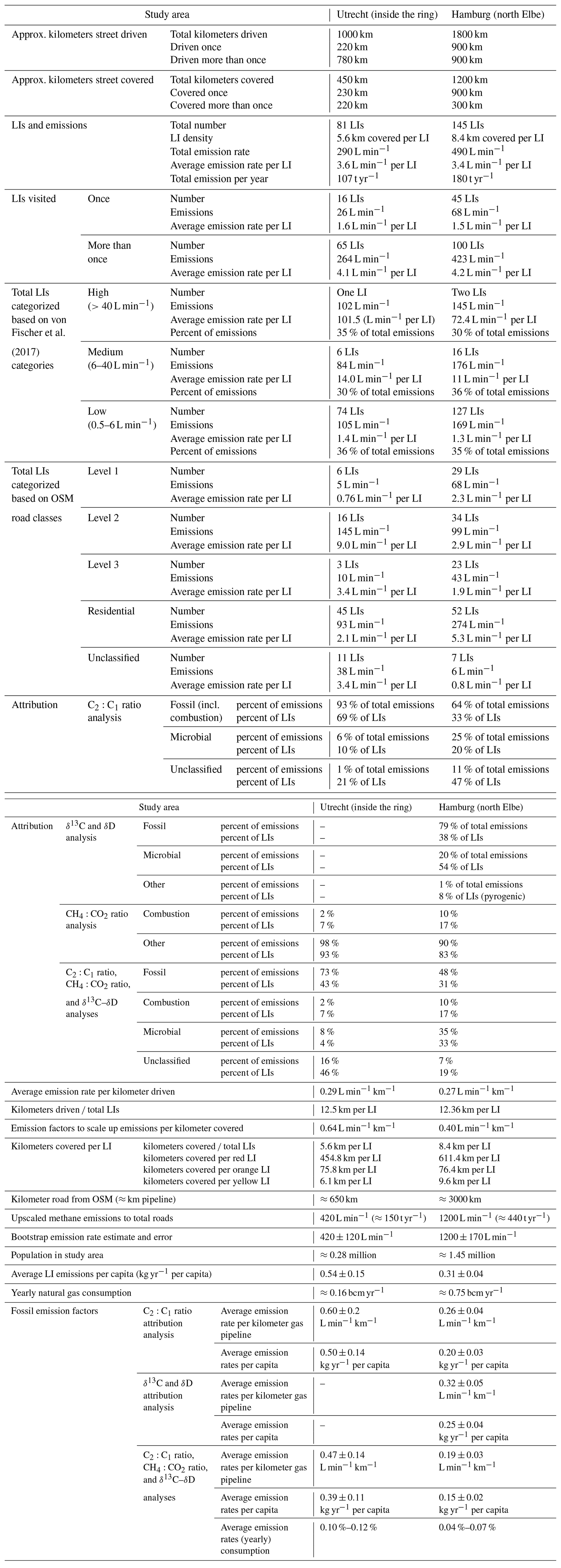
The distribution of CH4 LIs across the cities of Utrecht and Hamburg is shown in Fig. 2. As shown in Table 2, a total of 145 significant LIs were detected in Hamburg and 81 in Utrecht; these LIs cover all three LI categories. Two LIs in Hamburg and one LI in Utrecht fall in the high (red) emission category; the highest LI detected in Utrecht and Hamburg corresponded to emission rates of ≈100 and ≈70 L min−1, respectively. It has been noted that estimates for individual leaks with the Weller et al. (2019) algorithm can have large error; thus, these results are indicative of large leaks, but the precise emission strength is very uncertain. Six LIs in Utrecht and 16 LIs in Hamburg fall in the middle (orange) emission category, and 127 LIs in Hamburg and 74 LIs in Utrecht fall in the low (yellow) emission category. The distribution of emissions over the three categories is also similar between the two cities, with roughly one-third of the emissions originating from each category (Fig. 2), but the number of LIs in each category is different. The contribution of LIs in the high emission category is about a third of the total observed emissions – 35 % in Utrecht (one LI) and 30 % in Hamburg (two LIs).
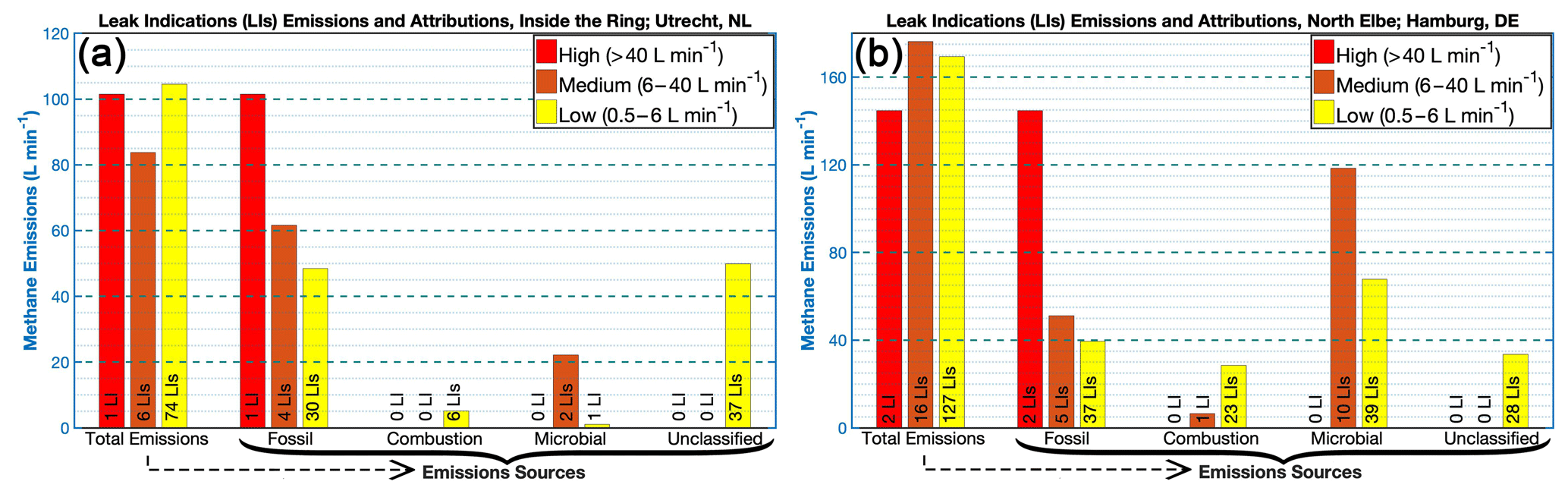
Figure 2Total CH4 emission rates from different sources in (a) Utrecht and (b) Hamburg; the arrow shows how the emissions are attributed to different sources.
CH4-emitting locations were categorized based on the roads where the LIs were observed (Figs. 1–3 and Table S8 in Sect. S3.1). Average emission rates per LI as derived from Eq. (1) are similar for the two cities with 3.6 L min−1 per LI in Utrecht and 3.4 L min−1 per LI in Hamburg, but they are distributed differently across the road (Fig. 3). In Utrecht, emitting locations on level 2 roads contributed the most (50 % of emissions) to the total emissions, while in Hamburg the majority of the emissions occurred on residential roads (56 % of total emissions). This shows that the major leak indications may happen on different road classes in different cities, and there is no general relation to the size of streets between these two cities.
Figure 3Total CH4 emissions in Utrecht and Hamburg; the arrow shows how the total emissions are distributed on different road classes.
In Fig. 4, we compare cumulative CH4 emissions for Utrecht and Hamburg to numerous US cities (Weller et al., 2019). After ranking the LIs from largest to smallest, it becomes evident that the largest 5 % of the LIs account for about 60 % of emissions in Utrecht and 50 % of the emissions in Hamburg.

Figure 4Cumulative plot of CH4 emissions across US cities, Utrecht, and Hamburg; datasets for the US cities are from Weller et al. (2019).
As mentioned above, the observed total emission rates observed on roads in an urban environment in the two cities are relatively similar when normalized by the total kilometers covered: 0.64 L min−1 km−1 for Utrecht and 0.4 L min−1 km−1 for Hamburg (Table 2). Using these two emission factors, the observed emission rates (≈110 t yr−1 in Utrecht and ≈180 t yr−1 in Hamburg) were upscaled to the entire road network in the two cities: ≈650 km in Utrecht and ≈3000 km in Hamburg. This includes the implicit assumption that the pipeline network is similar to the street network. Total upscaled emission rates based on mobile measurements on roads in an urban environment before considering attribution analysis over LI locations are 150 and 440 t yr−1 across the study areas of Utrecht and Hamburg, respectively. Distributing the calculated emission rates over the population in the city areas yields emission rates of 0.54±0.15 kg yr−1 per capita for Utrecht and 0.31±0.04 kg yr−1 per capita for Hamburg (see Sect. S3.2, Fig. S14).
3.2 Attribution of CH4 emissions across Utrecht and Hamburg
Figure 5 shows the results of the isotope analysis for the 21 locations in Hamburg where acceptable Keeling plots were obtained (see Sect. S3.3, Tables S9 and S10). The results cluster mostly in three groups, which are characterized by the expected isotope signatures for fossil, microbial, and pyrogenic samples as described in Röckmann et al. (2016).
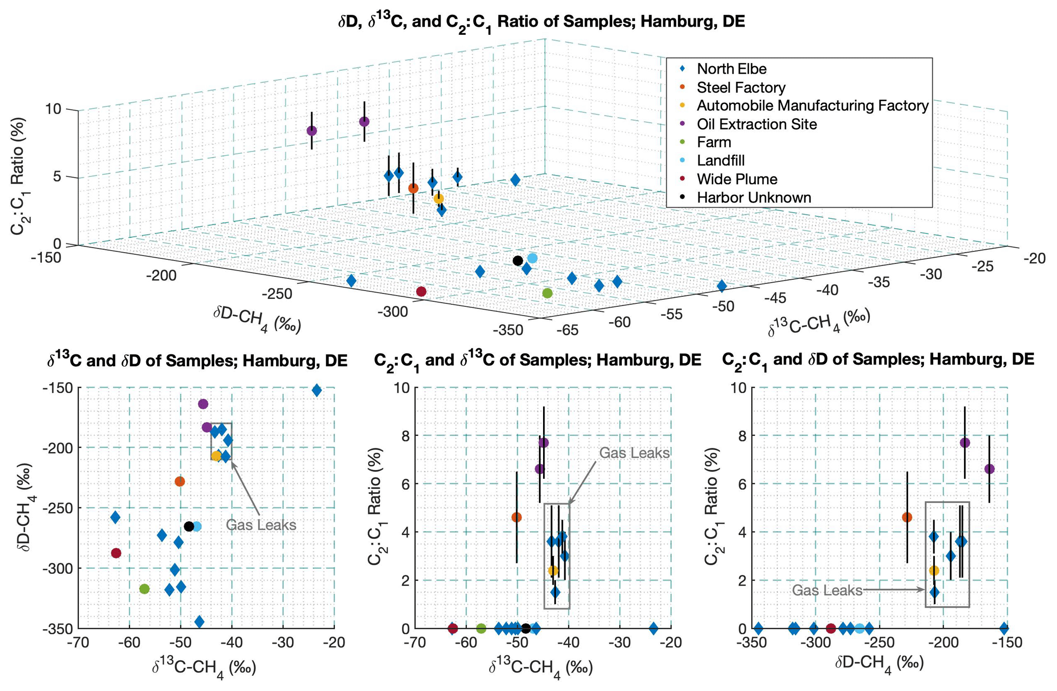
Figure 5Results from the attribution measurements in Hamburg: C2:C1 ratios and isotopic signatures (δ13C and δD) of collected air samples; measurement uncertainty in δ13C is 0.05 ‰–0.1 ‰ and in δD 2 ‰–5 ‰.
Average isotope signatures for the LIs in the city of Hamburg were ‰ and ‰ for the samples characterized as microbial and ‰ and ‰ for the samples characterized as fossil (Fig. 5). One sample from the Hamburg city area displays a very high source signature of ‰ and ‰. The origin of CH4, with such an unusual isotopic signature, could not be identified and is considered an outlier. In Hamburg, 10 % of the LI locations (38 % of emissions) on the north side of the Elbe were sampled for isotope analysis. The lab isotopic attributions show that the LIs with the higher emission rates are mostly caused by emissions of fossil CH4. A total of 79 % of the inferred emissions at 38 % of the LIs were identified as of fossil origin, 20 % of emissions at 54 % of the LIs as of microbial origin (for an identified source see Sect. S3.3, Fig. S15), and 1 % of emissions at 8 % of LIs as of pyrogenic origin.
In Hamburg, during three passes through the new Elbe tunnel (see Sect. S3.4, Fig. S16) a CH4:CO2 ratio of 0.2±0.1 ppb ppm−1 was derived for combustion-related emissions. During the surveys of open roads, clear CH4:CO2 correlations were observed for several LIs, and an example of a measurement of car exhaust is shown in Fig. S12a (see Sect. S2.6) with ppb ppm−1. Previous studies have shown relatively low CH4:CO2 ratios of ppb ppm−1 (Popa et al., 2014), 0.41 ppb ppm−1 (Nam et al., 2004), and 0.3 ppb ppm−1 (Naus et al., 2018) when cars work under normal conditions. During cold-engine (Naus et al., 2018) or incomplete combustion conditions, the fuel-to-air ratio is too high, which results in enhanced emissions of black carbon particles, reduced carbon compounds, and therefore higher CH4:CO2 ratios. Hu et al. (2018) reported 2±2.1 ppb ppm−1 in a tunnel but 12±5.3 ppb ppm−1 on roads. In addition to car exhaust, there are other combustion sources that can affect CH4 and CO2 mole fractions at the street level, including natural gas water heaters (CH4:CO2 ratio of ≈2 ppb ppm−1; Lebel et al., 2020) and restaurant kitchens. Based on the CH4:CO2 ratio (ppb ppm−1) criterion defined above (see Sect. 2.3.1), 17 % of LIs (10 % of emissions) can be attributed to combustion (see Sect. S3.4, Fig. S17) with a mean CH4:CO2 ratio of 3.2±3.9 ppb ppm−1 (max = 18.7 and min = 0.8 ppb ppm−1). The C2:C1 ratio for these LIs attributed to combustion in Hamburg was 7.8±3.5 %. In Utrecht 7 % of LIs (2 % of emissions) are attributed to combustion with a mean CH4:CO2 ratio of 9.8±5.8 ppb ppm−1 (max = 16.7 and min = 3.0 ppb ppm−1).
Based on the C2H6 signals, 64 % of the emissions (33 % of LIs) were characterized as fossil, while 25 % of emissions (20 % of LIs) were identified as microbial. Due to low CH4 and C2H6 enhancements, 47 % of the locations (11 % of emissions) were considered unclassified. The C2:C1 ratio for the LIs attributed to emissions from NGDNs in the Hamburg study area (north Elbe) is 4.1±2.0 %. The oil production site in southeast Hamburg had a higher C2:C1 ratio of 7.1±1.5 %.
Figure 6CH4 enhancements measured downwind of the waste water treatment plant on Brailledreef Street and later used for quantifications from this facility in Utrecht; the center of the area where the sludge treatment is located was considered the effective CH4 emission source. The plumes are plotted on the same scale, and maximum CH4 enhancement is ≈0.3 ppm.
In Utrecht, C2H6 was measured only during four surveys in February, April, and June 2019 (revisits of 2 d surveys across the city center and 2 d to LIs with high emission rates) as the CH4–C2H6 analyzer was not available during the first campaign. The C2:C1 ratios from this limited survey indicate that 93 % of emissions (69 % of the LIs across the city center, including combustion) are likely from fossil sources (Table 2) and 73 % of emissions (43 % of the LIs, including combustion) out of all LIs. In Utrecht, the C2:C1 ratio for the LIs attributed to NGDNs is 3.9±0.8 %.
3.3 Quantification of CH4 plume from larger facilities
Table 3 shows the emission rate estimates from the larger facilities in Utrecht and Hamburg. CH4 plumes from the WWTP (Fig. 6 and in Sect. S1.6., Table S5) were intercepted numerous times during the city transects, and the error estimate in Table 3 represents 1 standard deviation of five sets of measurements; each measurement comprises two to four transects during three measurement days (12 February 2018, 24 April 2018, and 7 January 2019). Figure 7 shows an example of a fit of a Gaussian plume to the measurements from the Utrecht WWTP. The derived distance to the source was 215±90 m, the hourly average wind speed was 3.5±1.1 m s−1, and the wind direction was 178±5∘ (see Sect. S1.6, Table S5).
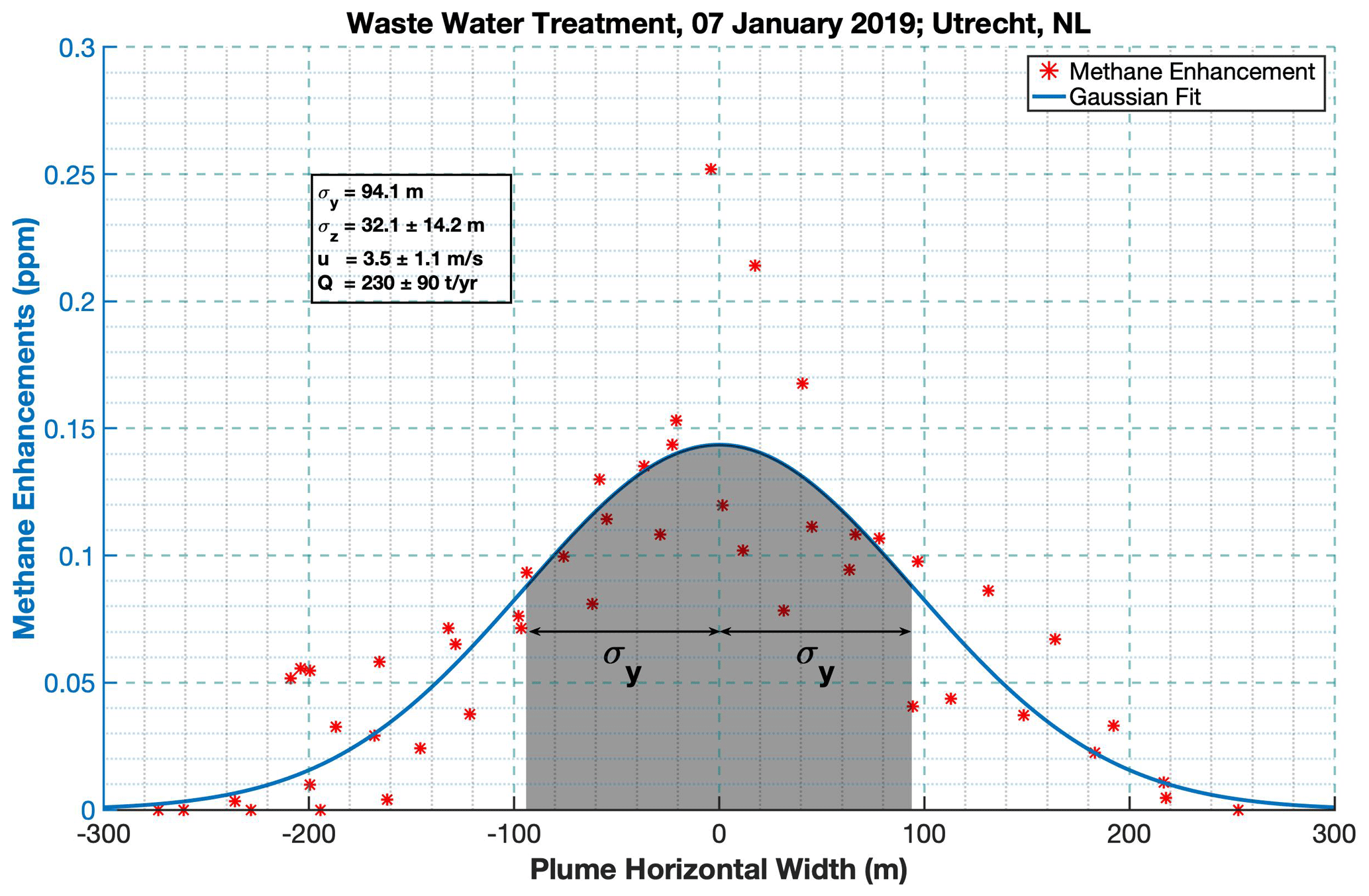
Figure 7Gaussian curve fitted to some transects downwind of the waste water treatment plant in Utrecht.
Table 3CH4 emissions from larger facilities in Utrecht and Hamburg estimated with the Gaussian plume model.
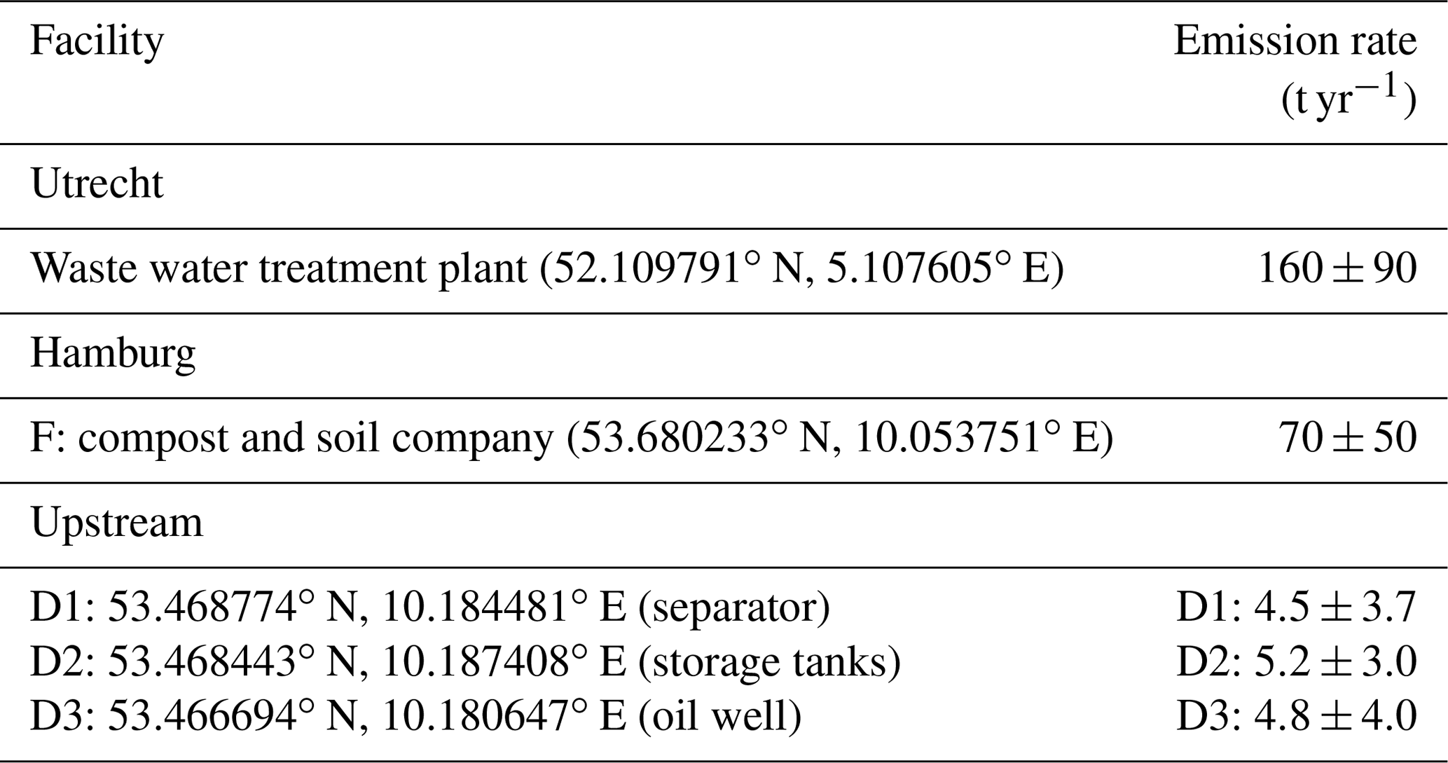
The total emission rate of the WWTP in Utrecht was estimated at 160±90 t yr−1. The reported errors include stability classes, wind speed and direction, and effective point source coordinates. Not all transects provided datasets that allowed an adequate Gaussian fit, and these were not included in total estimates from the facilities; e.g., measurements during the visits to the harbor area in Hamburg were excluded. In Hamburg, plumes from several facilities were also intercepted several times (see Sect. S1.6, Table S6). For a compost and soil company in Hamburg we estimate an emission rate of 70±50 t yr−1. The mobile quantifications at the upstream sites in Hamburg from a separator, a tank, and an oil well yield annual CH4 emissions of 4.5±3.7, 5.2±3.0, and 4.8±4.0 t yr−1, respectively.
4.1 Detection and quantification
As mentioned above (see Sect. 2.2.2), we used methods similar to the ones introduced by von Fischer et al. (2017) and updated in Weller et al. (2019) that were used to characterize CH4 emissions from local gas distribution systems in the US. An important difference is that we did not visit each street twice in the untargeted survey, and the revisits were specifically targeted at locations where we had found an LI during the first visit. A consequence of the different sampling strategy is that we do not base our city-level extrapolated emissions estimates on “confirmed” LIs, as done in Weller et al. (2019), but on all the LIs observed. In our study, 60 % of CH4 LIs in Utrecht and 46 % of LIs in Hamburg were confirmed. This number may be biased high, since we preferentially revisited locations that had shown higher LIs, and the percentage of confirmed LIs may have been lower if we had visited locations with smaller LIs. Von Fischer et al. (2017) reported that LIs in the high emission rate category have a 74 % chance of detection, which decreased to 63 % for the middle category and 35 % for the small category. In our study, all LIs within the high emission rate category (n=1 and n=2 LIs in Utrecht and Hamburg, respectively) were confirmed in both cities. Overall, the confirmation rates found in Hamburg and Utrecht were similar to the ones reported in the US cities by von Fischer et al. (2017), suggesting that the results from both driving strategies can be compared when we take into account an overall confirmation percentage of roughly 50 %.
In 13 US cities the “LI density” ranged from one LI per 1.6 km driven to one LI per ≈320 km driven (EDF, 2019). This illustrates that cities within one country can be very different in their NGDN infrastructure. In Utrecht, one LI was observed every 5.6 km of street covered and in Hamburg every 8.4 km covered. Note that we normalize the number of LIs per kilometer of road covered, not kilometers of road driven, since the revisits were targeted to confirm LIs, which would bias the statistics if we normalized by kilometers of road driven. After accounting for the confirmation percentage of 50 %, the LI densities in Utrecht and Hamburg become one LI per 11.2 km covered in Utrecht and one LI per 16.8 km covered in Hamburg. When we take into account the attributions (the fraction of fossil to total LIs is 43 % in Utrecht and 31 % in Hamburg), confirmed LIs from the NGDN are found every 26 km in Utrecht and every 54 km in Hamburg. The highest 1 % of the LIs in Utrecht and Hamburg account for approximately 30 % of emissions, emphasizing the presence of a skewed distribution of emissions. The emissions distribution is even more skewed for these two European cities than for countrywide US cities, where approximately 25 % of emissions come from the highest 5 % of the LIs. Skewed emission distributions appear to be typical for emissions from the oil and gas supply chain across different scales. For example, a synthesis study reviewing the distribution of upstream emissions from the US natural gas system shows that in the US 5 % of the leaks are responsible for 50 % of the emissions (Brandt et al., 2016).
4.2 Attribution
Four different approaches were combined in Hamburg for emission source attribution, which allows an evaluation of their molecular consistency. Figure 5 shows that measurements of C2:C1, δD, and δ13C provide a very consistent distinction between fossil and microbial sources of CH4. Except for one outlier with very enriched δ13C and δD contents and no C2H6 signal, all samples that are classified as “microbial” and depleted in δ13C and δD signatures contain no measurable C2H6. Samples that are characterized as “fossil”, based on δ13C and δD signatures, bear a C2H6 concomitant signal. This strengthens the confidence in source attribution using these tracers. The fossil δ13C signature of bag samples from natural gas leaks in Hamburg ( ‰) is higher than recent reports from the city of Heidelberg, Germany ( ‰; Hoheisel et al., 2019). This shows that within one country, δ13C from NGDNs can vary from one region to another. These numbers do not agree within combined errors but are also not very different. δ13C values of CH4 from the NGDN can vary regionally and temporally, e.g., due to differences in the mixture of natural gas from various suppliers for different regions in Germany (DVGW, 2013). In a comprehensive study at the global scale, it is also shown that δ13C values of fossil fuel CH4 have significant variabilities in different regions within an individual basin (Fig. 4 in Sherwood et al., 2017).
In Hamburg both C2:C1 and CH4:CO2 analyses along with δ13C and δD signatures suggest that ≈50 % to ≈80 % of estimated emissions (≈30 % and ≈40 % of LIs, respectively) originate from NGDNs, whereas CH4:CO2 analysis and the smaller sample of C2:C1 measurements in Utrecht suggest that the overwhelming fraction (70 %–90 % of emissions; 40 %–70 % of LIs) originated from NGDNs. We note that although it is widely assumed that microbial CH4 is not associated with ethane, some studies have reported microbial production of ethane, so it may not be a unique identifier (Davis and Squires, 1954; Fukuda et al., 1984; Gollakota and Jayalakshmi, 1983; Formolo, 2010). The online C2:C1 analysis to attribute LIs is fast and can be used at a larger scale, but with the instrument we used we were not able to clearly attribute sources with CH4 enhancements of less than 500 ppb. Isotopic analysis by IRMS can attribute sources for smaller LIs (down to 100–200 ppb) but is clearly more labor-intensive, and it would be a considerable effort to take samples from all LIs observed across an urban area. Overall, C2H6 and CO2 signals are very useful in eliminating non-fossil LIs in mobile urban measurements, and with improvements in instrumentations=, analyzing signals of these two species along with evaluation of CH4 signals can make the process of detecting pipeline leaks from NGDNs more efficient.
In Hamburg, most of the LIs were detected in the city center (Fig. 1). This means that the LI density is higher than the average value in the center, but much lower than the average value in the surrounding districts and residential areas. Many of the LIs in the city center were attributed to combustion and microbial sources; thus, they do not originate from leaks in the NGDN. Many of the microbial LIs encountered in Hamburg are around the Binnenalster lake (see Sect. S3.3, Fig. S15), which suggests that anaerobic methanogenesis (Stephenson and Stickland, 1933; Thauer, 1998) can cause microbial emissions in this lake, as seen in other studies focused on emissions from other lakes (e.g., DelSontro et al., 2018; Townsend-Small et al., 2016). Microbial CH4 emissions from the sewage system (Guisasola et al., 2008) can also be an important source in this area, as seen in US urban cities (Fries et al., 2018). Fries et al. (2018) performed direct measurement of CH4 and nitrous oxide (N2O) from a total of 104 sites, analyzed δ13C and δD signatures of samples from 27 of these locations, and attributed 47 % of these locations to microbial emissions in Cincinnati, Ohio, USA.
4.3 Comparison to national inventory reports
In national inventory reports, total upscaled emissions from NGDNs are based on sets of emission factors for different pipeline materials (e.g., grey cast iron, steel, or plastic) at different pressures (e.g., mbar or >200 mbar). The reported emission factors are based on the IPCC tier 3 approach (IPCC: Intergovernmental Panel on Climate Change; Buendia et al., 2019). However, emission estimates do not exist for individual cities, including Utrecht and Hamburg. Also, it is not possible to calculate a robust city-level estimate using the nationally reported emission factors because there are no publicly available associated activity data, i.e., pipeline materials and lengths for each material, at the level of individual cities. As a result, a robust direct comparison between nationally reported emissions and our measurements, akin to a recent study in the United States (Weller et al., 2020), is currently not possible. The following juxtaposition of our estimates and national inventory downscaling to the city level is therefore provided primarily as an illustration of the data gaps rather than a scientific comparison. In Utrecht, we attributed 70 %–90 % of the mobile-measurement-inferred emissions of ≈150 t yr−1 to the NGDN, thus 105–135 t yr−1.
The Netherlands National Institute for Public Health and the Environment (RIVM) inventory report derived an average NGDN emission factor of ≈110 kg km−1 yr−1 using 65 leak measurements from different pipeline materials and pressures in 2013. This weighted average ranged from a maximum of 230 kg km−1 yr−1 for grey cast iron pipelines to a minimum of 40 kg km−1 yr−1 for pipelines of other materials with overpressures 200 mbar (for details, see p. 130 in Peek et al., 2019). This results in average CH4 emissions of ≈70 t yr−1 (min = 30 t yr−1 and max = 150 t yr−1) for the study area of Utrecht, assuming ≈650 km of pipelines inside the ring and further assuming that Utrecht's NGDN is representative of the national reported average (see qualifiers above). The average emissions for the Utrecht study, based on emissions factors reported for the Netherlands, is smaller by a factor of 1.5–2 compared to the emissions derived here. The variability factor of 5, from the reported emissions (resulting from the variability in pipeline materials), highlights the need for city-level specific activity data for a robust comparison. In Hamburg, 50 %–80 % of the upscaled emissions of 440 t yr−1 (220–350 t yr−1) can be attributed to emissions from the NGDN. The national inventory from the Federal Environment Agency (UBA) in Germany reports an average CH4 emission factor for NGDNs from low-pressure pipelines of ≈290 kg km−1 yr−1 (max = 445 kg km−1 yr−1 for grey cast iron and min = 51 kg km−1 yr−1 for plastic) based on measurements from the 1990s (Table 169 in Federal Environment Agency, 2019). Assuming ≈3000 km of pipelines in the targeted region, and further assuming that Hamburg's NGDN is representative of the national reported average (see qualifiers above), results in an estimated NGDN CH4 emissions average of ≈870 t yr−1 (min = 155 t yr−1 and max = 1350 t yr−1). While this study's estimate (220–350 t yr−1) falls in the lower end of this range, the reported emissions variability factor of 9 (resulting from the variability in pipeline materials) again highlights the need for city-level specific activity data for a robust comparison. To put the national inventory comparison into perspective, it should be noted that GasNetz Hamburg detected and fixed leaks for 20 % of the fossil LIs in this study, which accounted for 50 % of emissions. In Utrecht and Hamburg, the natural gas consumption in our target areas was retrieved through communications with LDCs. In the Utrecht and Hamburg study areas, natural gas consumption is 0.16 bcm yr−1 (STEDIN, personal communication, 2020) and 0.75 bcm yr−1 (GasNetz Hamburg, personal communication, 2020), respectively. The estimated emissions from NGDNs in our study are between 0.10 % and 0.12 % in Utrecht and between 0.04 % and 0.07 % in Hamburg for total annual natural gas consumption in the same area. In the US, where the majority of natural gas consumption is from residential and commercial sectors, Weller et al. (2020) reported emissions of 0.69 Tg yr−1 (0.25–1.23 with a 95 % confidence interval), with a sum of ≈170 Tg yr−1 (US EIA, 2019), showing a 0.4 % (0.15 %–0.7 %) loss from NGDNs. The US NGDN loss is about 4 times larger than our reported loss in Utrecht and is about 10 times larger than the loss for Hamburg. Considering the population of Utrecht (≈0.28 million) and Hamburg (≈1.45 million), the natural gas consumption densities in these study areas are ≈570 and ≈520 m3 yr−1 per capita; in the US (population ≈330 million; US Census Bureau, 2020) the density is about ≈730 m3 yr−1 per capita (see Sect. S3.2, Fig. S14). This shows that annual natural gas consumption per capita in the US is about 30 % and 40 % higher than in Utrecht and Hamburg, respectively. The emission per kilometer of pipeline in Utrecht is between 0.45 and 0.5 L min−1 km−1 and in Hamburg between 0.2 and 0.32 L min−1 km−1. In the US, based on 2 086 000 km of local NGDN pipeline (Weller et al., 2020), this emission factor will be between 0.32 and 1.57 L min−1 km−1. This shows higher emissions per kilometer of pipeline in countrywide studies in the US compared to just the two European cities of Utrecht and Hamburg (see qualifiers above). This can be partly explained by pipeline material, maintenance protocols, and higher use of natural gas consumption in the US. However, the substantial variability in emission rates across US cities, as well as the annual variability of gas consumption over the year, again restricts a direct comparison of two cities with a national average measured over multiple years.
Normalized LI emissions per capita in Utrecht (0.54±0.15 kg yr−1 per capita) are almost double the emission factor in Hamburg (0.31±0.04 kg yr−1 per capita). This metric may be useful to compare cities, assuming that the emission quantification method is equally effective for different cities. CH4 emissions can vary among different cities, depending on the age, management, and material of NGDNs and/or the management of local sewer systems. In our study, we only surveyed two cities, and the above number may not be adequate for extrapolation to the country scale (McKain et al., 2015).
4.4 Interaction with utilities
After the city surveys, locations with the highest emissions (high and medium categories) were shared with STEDIN Utrecht, and all LI locations were reported to GasNetz Hamburg. The utilities repair teams were sent to check whether LIs could be detected as leaks from the NGDN and fixed. The LDCs follow leak detection procedures based on country regulations (e.g., for GasNetz Hamburg, see Sect. S4.1, Table S11). GasNetz Hamburg also co-located the coordinates of the detected and reported LIs with the NGDN and prioritized repairs based on the safety regulations mentioned in Table S12 (see Sect. S4.1). This interaction with the LDCs resulted in fixing major NGDN leaks in both cities. In Utrecht the only spot in the high emission category was reported to STEDIN, but the pipelines on this street had been replaced, which most likely fixed the leak, as it was not found later by the gas company or in our later survey with the CH4–C2H6 analyzer. In Utrecht, half of the LIs in the medium category were found and repaired.
A routine leak survey (detection and repair) had been performed by GasNetz Hamburg 1–5 months before the campaign for the different regions (see Sect. S4.1, Table S11). The timing of any routine detection and repair likely influences the absolute number of LIs measured during independent mobile measurements, and the survey by GasNetz Hamburg thus likely influenced the absolute number of LIs measured in our campaign. We then reported the LI latitude–longitude coordinates to GasNetz Hamburg about 4 months after our campaign. Additionally, we provided map images of the LIs immediately after the campaign. The comparison of the number of reported LIs (and emission rates) during our campaign with those identified by GasNetz Hamburg post-campaign assumes that the leaks continued to emit gas until they were detected and fixed by GasNetz Hamburg (if they were detected).
Depending on how close the gas leaks are located to a building, the LDCs prioritize the leaks into four classes from the highest to lowest priority: A1, A2, B, and C (see Sect. S4.1, Table S12). In Hamburg, both LIs in the high category were identified as A1 gas leaks and fixed by GasNetz Hamburg immediately. Most of the Hamburg LIs that were detected and identified as fossil are in close proximity to the natural gas distribution pipelines (see Sect. S4.2, Table S13). Investigation of the pipeline material shows that most of NGDN emissions are due to leaks from steel pipelines (see Sect. S4.2, Table S14), which are more prone to leakage because of pipeline corrosion (Zhao et al., 2018). Nevertheless, only 7 of the 30 LIs (23 %) that were positively attributed to fossil CH4 were detected and fixed by the LDC. If we assume that the fraction of fossil to total LIs determined in Hamburg (≈35 %) is representative for the entire population of LIs encountered (thus also for the ones that were not attributable), about 50 of the 145 LIs are likely due to fossil CH4. The LDC found and fixed leaks at 10 of these locations (≈20 %). A recent revisit (January 2020) to these locations confirmed that no LIs were detected at 9 out of these 10 locations. For the 10th location a smaller LI was detected in close proximity, and GasNetz Hamburg confirmed that this was a leak from a steel pipeline. The whole pipeline system on this street dates back to the 1930s and is targeted for replacement in the near future.
In summary, about 20 % of the LIs, including the two largest LIs that were attributed to a fossil source, were identified as NGDN gas leaks (see Sect. S4.2, Fig. S18) and were repaired by GasNetz Hamburg, but these accounted for about 50 % of fossil CH4 emissions in Hamburg, similar to what was observed in the US studies (Weller et al., 2018). Possibly, smaller leakages that can be detected with the high-sensitivity instruments used in mobile surveys cannot be detected with the less sensitive equipment of LDCs. Another possible explanation for the fact that the LDC did not detect more leaks may be that reported LI locations do not always coincide with the actual leak locations, although Weller et al. (2018) reported that the median distance of actual leak locations to the reported ones was 19 m. Combined measurements with GasNetz Hamburg are planned to investigate why the majority of the smaller LIs reported in mobile surveys are not detected in the regular surveys of the LDC.
The average C2:C1 ratio for LIs with a significant C2H6 signals across Hamburg was 5.6±3.9 %. For the spots where the LDC found and fixed leaks this ratio was 3.9±2.6 %. Thus, some of the locations where CH4 enhancements were found were influenced by sources with an even higher C2:C1 ratio than the gas in the NGDN. One confirmed example is the very high ratio found in exhaust from a vehicle as shown in Fig. S12 (see Sect. S2.6). The abnormal operation of this vehicle is confirmed by the very high CH4:CO2 ratio of 5.5 ppb ppm−1 (Sect. S2). This is more than 20 times higher than the CH4:CO2 ratios of 0.2±0.1 ppb ppm−1 observed during passages through the Elbe tunnel, a ratio that agrees with previous studies (Sect. S2).
Repairing gas leaks in a city has several benefits for safety (preventing explosions), sustainability (minimizing GHG emissions), and economics. Gas that is not lost via leaks can be sold for profit, but gas leak detection and repair are expensive and usually associated with interruptions of the infrastructure (breaking up pavements and roads). Also, as reported above, and in agreement with the studies in US cities, for small LIs the underlying leaks are often not found by the LDCs, possibly because their equipment is less sensitive and aimed at finding leak rates that are potentially dangerous.
Our measurements in Hamburg demonstrate that smaller LIs in particular may originate from biogenic sources, e.g., the sewage system, and not necessarily from leaks in the NGDN. In this respect, attribution of LIs prior to reporting to the LDCs may be beneficial to facilitate effective repair. Figure S19 (see Sect. S5) illustrates how the individual measurement components can be efficiently combined in a city leak survey program.
4.5 Large facilities
The WWTP in Utrecht emits 160±90 t yr−1, which is similar to the total detected emissions (150 t yr−1) inside the study area of Utrecht. The emissions reported for this facility from 2010 until 2017 are 130±50 t yr−1 (Rijksoverheid, 2019), in good agreement with our measurements. CH4 emissions from a single well in Hamburg were estimated at 4.4±3.5 t yr−1, which is in the range of median emissions of 2.3 t yr−1 reported for gas production wells in Groningen, NL (Yacovitch et al., 2018), and average emissions of all US oil and gas production wells of 7.9±1.8 t yr−1 (Alvarez et al., 2018). In Hamburg, the emissions from a compost and soil company amount to about 10 % of the total emissions in the city target region, whereas a wellhead, a storage tank, and a waste–oil separator contribute only about 1 % each. This shows that individual facilities can contribute significantly to the total emissions of a city. The contribution of each source is dependent on infrastructure, urban planning, and other conditions in the city (e.g., age and material of the pipeline, maintenance programs, waste management, sewer system conditions), which may change the source mix from one city to another. For example, in Utrecht the WWTP is located within our domain of study. The wastewater treatment in Hamburg most likely causes CH4 emissions elsewhere. Therefore, facility-scale CH4 emissions should be reported on a more aggregated provincial or national level. For emissions from the NGDN, the urban scale is highly relevant, as emissions can only be mitigated at this scale.
Mobile measurements provide a fast and accurate technique for observing and identifying even relatively small CH4 enhancements (i.e., tens of parts per billion) across cities and are useful for detecting potential gas leaks. During our intensive measurement campaigns, 81 LIs were observed in Utrecht (corresponding to emissions of ≈110 t CH4 yr−1) and 145 LIs (≈180 t CH4 yr−1) in Hamburg. These estimates, based on the streets covered, were then upscaled to the total study area using the road network map as a proxy for the length of the pipeline network, which then yielded total emissions of 150 and 440 t yr−1 across the study area of Utrecht and Hamburg, respectively. The isotopic signature of CH4 in air samples and continuous mobile measurement of CO2 and C2H6 mole fraction show that not all the LIs observed across the two cities have a fossil origin. In Utrecht, C2:C1 and CH4:CO2 analyses show that 70 %–90 % of emissions were fossil. In Hamburg, C2:C1, CH4:CO2, and δ13C–δD analyses suggest that 50 %–80 % of emissions originate from natural gas pipelines. For the locations where samples for isotope analysis were collected, 80 % of emissions were identified as fossil. A large fraction of emissions in both cities originated from a few high-emitting locations. The LDC in Hamburg (GasNetz Hamburg) detected and fixed leaks at 20 % of the locations that are likely due to fossil sources, but these accounted for 50 % of emissions. Large LIs were generally confirmed as gas leaks from steel pipelines. The C2:C1 ratio at the locations where gas leaks were fixed by GasNetz Hamburg was 3.9±2.6 %. The mobile measurement technique is less labor- and time-intensive than conventional methods and can provide extensive coverage across a city in a short period. Based on our experience for the Netherlands and Germany a protocol could be developed that aids LDCs in guiding their leak detection and repair teams. The use of emission categories and source attribution can help target repair activities to the locations of large fossil emissions. Emission quantification from large facilities shows that these emissions may be equivalent to total CH4 emissions from NGDN leaks in urban environments. In order to analyze discrepancies between spatially explicit measurement-based estimates as presented here and reported annual average national emissions by sector, a coordinated effort with national agencies is necessary to address the lack of publicly available activity data (e.g., pipe material) disaggregated from the national level (e.g., at the city level).
A MATLAB® code to analyze urban surveys is available on GitHub from Maazallahi et al. (2020a).
The data, including in situ measurements, GPS data, and boundaries of study areas, are available on the Integrated Carbon Observation System (ICOS) portal from Maazallahi et al. (2020b).
A virtual tour of the measurements is available on the Leibniz Information Centre for Science and Technology and University Library (TIB) portal from Maazallahi et al. (2020c).
The supplement related to this article is available online at: https://doi.org/10.5194/acp-20-14717-2020-supplement.
HM performed the mobile measurements, wrote the MATLAB® code, analyzed the data, and together with TR drafted the paper. JMF and MM contributed with air sampling and isotope analysis. DZA and SS contributed to the scientific interpretation and comparison between European and US cities. ZDW and JCvF facilitated comparison to US cities and contributed to the statistical analysis. HDvdG and TR provided instruments and equipment as well as supervising the measurements and data analysis. TR developed the research idea and coordinated the city campaigns. All authors contributed to the interpretation of the results and the improvement of the paper.
The authors declare that they have no conflict of interest.
This work was supported by the Climate and Clean Air Coalition (CCAC) Oil and Gas Methane Science Studies (MMS) hosted by the United Nations Environment Programme. Funding was provided by the Environmental Defense Fund, the Oil and Gas Climate Initiative, the European Commission, and CCAC. This project received further support from the H2020 Marie Skłodowska-Curie project Methane goes Mobile – Measurements and Modelling (MEMO2; https://h2020-memo2.eu/, last access: 30 November 2020), grant number 722479. Daniel Zavala-Araiza and Stefan Schwietzke were funded by the Robertson Foundation. We thank Rebecca Fisher, who supervised the RHUL contribution to the isotopic analysis for the Hamburg campaign. Special thanks to Stefan Bühler from the Meteorological Institute of Hamburg University and Stefan Kinne from the Max Planck Institute for Meteorology for hosting our team during the Hamburg city measurement surveys. We would like to extend our appreciation to the anonymous referees for the insightful comments, which led to improvements of the paper. We appreciate continuous efforts from the executive and management board of GasNetz Hamburg along with Luise Westphal, Michael Dammann, Ralf Luy, and Christian Feickert, who facilitated productive communications, provided information on the gas infrastructure in Hamburg, and organized leak repairs with their teams in the study area in Hamburg. We also thank the asset manager of STEDIN Utrecht, Ricardo Verhoeve, who provided information and planned leak repairs by STEDIN in Utrecht. We thank Charlotte Große from DBI Gas and Environmental Technologies GmbH Leipzig (DBI GUT Leipzig), who helped with clarifying information on reported emission factors provided in national inventory reports. We thank the former MSc students of Utrecht University, Laurens Stoop and Tim van den Akker, who helped with the measurements in the Utrecht study area.
This research has been supported by the Environmental Defense Fund, the Oil and Gas Climate Initiative, the European Commission, CCAC (grant no. 1043-000011-11070-100-00), and the H2020 Marie Skłodowska-Curie project Methane goes Mobile – Measurements and Modelling (grant no. 722479).
This paper was edited by Eliza Harris and reviewed by two anonymous referees.
ACM: Authority for Consumers and Markets in the Netherlands, Low NOx Burgners (LNBs) gas code, available at: https://wetten.overheid.nl/BWBR0037935/2018-05-26 (last access: 25 June 2020), 2018.
Allen, D. T., Torres, V. M., Thomas, J., Sullivan, D. W., Harrison, M., Hendler, A., Herndon, S. C., Kolb, C. E., Fraser, M. P., Hill, A. D., Lamb, B. K., Miskimins, J., Sawyer, R. F., and Seinfeld, J. H.: Measurements of methane emissions at natural gas production sites in the United States, P. Natl. Acad. Sci. USA, 110, 17768–17773, https://doi.org/10.1073/pnas.1304880110, 2013.
Alvarez, R. A., Zavala-Araiza, D., Lyon, D. R., Allen, D. T., Barkley, Z. R., Brandt, A. R., Davis, K. J., Herndon, S. C., Jacob, D. J., Karion, A., Kort, E. A., Lamb, B. K., Lauvaux, T., Maasakkers, J. D., Marchese, A. J., Omara, M., Pacala, S. W., Peischl, J., Robinson, A. L., Shepson, P. B., Sweeney, C., Townsend-Small, A., Wofsy, S. C., and Hamburg, S. P.: Assessment of methane emissions from the U.S. oil and gas supply chain, Science, 361, 186–188, https://doi.org/10.1126/science.aar7204, 2018.
Brandt, A. R., Heath, G. A., and Cooley, D.: Methane Leaks from Natural Gas Systems Follow Extreme Distributions, Environ. Sci. Technol., 50, 12512–12520, https://doi.org/10.1021/acs.est.6b04303, 2016.
Brantley, H. L., Hagler, G. S. W., Kimbrough, E. S., Williams, R. W., Mukerjee, S., and Neas, L. M.: Mobile air monitoring data-processing strategies and effects on spatial air pollution trends, Atmos. Meas. Tech., 7, 2169–2183, https://doi.org/10.5194/amt-7-2169-2014, 2014.
Brass, M. and Röckmann, T.: Continuous-flow isotope ratio mass spectrometry method for carbon and hydrogen isotope measurements on atmospheric methane, Atmos. Meas. Tech., 3, 1707–1721, https://doi.org/10.5194/amt-3-1707-2010, 2010.
Bright, E. A., Coleman, P. R., and Dobson, J. E.: LandScan: A Global Population database for estimating populations at risk, Photogram. Eng. Remote Sens., 66, 849–858, https://doi.org/10.1201/9781482264678-24, 2000.
Brümmer, B., Lange, I., and Konow, H.: Atmospheric boundary layer measurements at the 280 m high Hamburg weather mast 1995–2011: mean annual and diurnal cycles, Meteorol. Z., 21, 319–335, https://doi.org/10.1127/0941-2948/2012/0338, 2012.
Buendia, E. C., Guendehou, S., Limmeechokchai, B., Pipatti, R., Rojas, Y., Sturgiss, R., Tanabe, K., Wirth, T., Romano, D., Witi, J., Garg, A., Weitz, M. M., Cai, B., Ottinger, D. A., Dong, H., MacDonald, J. D., Ogle, S. M., Rocha, M. T., Sanchez, M. J. S., Bartram, D. M., and Towprayoon, S.: 2019 refinement to the 2006 IPCC guidelines for national greenhouse gas inventories, available at: https://www.ipcc.ch/report/2019-refinement-to-the-2006-ipcc-guidelines-for-national (last access: 4 June 2020), 2019.
Bukowiecki, N., Dommen, J., Prévôt, A. S. H., Richter, R., Weingartner, E., and Baltensperger, U.: A mobile pollutant measurement laboratory – Measuring gas phase and aerosol ambient concentrations with high spatial and temporal resolution, Atmos. Environ., 36, 5569–5579, https://doi.org/10.1016/S1352-2310(02)00694-5, 2002.
Caulton, D. R., Li, Q., Bou-Zeid, E., Fitts, J. P., Golston, L. M., Pan, D., Lu, J., Lane, H. M., Buchholz, B., Guo, X., McSpiritt, J., Wendt, L., and Zondlo, M. A.: Quantifying uncertainties from mobile-laboratory-derived emissions of well pads using inverse Gaussian methods, Atmos. Chem. Phys., 18, 15145–15168, https://doi.org/10.5194/acp-18-15145-2018, 2018.
Chamberlain, S. D., Ingraffea, A. R., and Sparks, J. P.: Sourcing methane and carbon dioxide emissions from a small city: Influence of natural gas leakage and combustion, Environ. Pollut., 218, 102–110, https://doi.org/10.1016/J.ENVPOL.2016.08.036, 2016.
Chen, J., Dietrich, F., Maazallahi, H., Forstmaier, A., Winkler, D., Hofmann, M. E. G., Denier van der Gon, H., and Röckmann, T.: Methane emissions from the Munich Oktoberfest, Atmos. Chem. Phys., 20, 3683–3696, https://doi.org/10.5194/acp-20-3683-2020, 2020.
Curran, S. J., Wagner, R. M., Graves, R. L., Keller, M., and Green, J. B.: Well-to-wheel analysis of direct and indirect use of natural gas in passenger vehicles, Energy, 75, 194–203, https://doi.org/10.1016/j.energy.2014.07.035, 2014.
Davis, J. B. and Squires, R. M.: Detection of Microbially Produced Gaseous Hydrocarbons Other than Methane, Science, 119, 381–382, https://doi.org/10.1126/science.119.3090.381, 1954.
DelSontro, T., Beaulieu, J. J., and Downing, J. A.: Greenhouse gas emissions from lakes and impoundments: Upscaling in the face of global change, Limnol. Oceanogr. Lett., 3, 64–75, https://doi.org/10.1002/lol2.10073, 2018.
DVGW: Technische Regel – ArbeitsblattDVGW G 260 (A), Bonn, available at: https://shop.wvgw.de/var/assets/leseprobe/508866_lp G 260.pdf (last access: 30 November 2020), 2013.
EDF: Local leaks impact global climate, available at: https://www.edf.org/climate/methanemaps, last access: 5 November 2019.
Efron, B.: Bootstrap Methods: Another Look at the Jackknife, Ann. Stat., 7, 1–26, https://doi.org/10.1214/aos/1176344552, 1979.
Efron, B.: The Jackknife, the Bootstrap and Other Resampling Plans, Society for Industrial and Applied Mathematics, Philadelphia, PA, USA, ISBN 978-0-89871-179-0, 1982.
Efron, B. and Tibshirani, R. J.: An Introduction to the Bootstrap, Champman & Hall, London, 1993.
EPA: User's guide for the industrial source guide complex (ISC3) dispersion models, in: volume II – Description of model algorithms, US Environmental Protection Agency Office of Air Quality Planning and Standards Emissions, Monitoring, and Analysis Division Research Triangle Park, North Carolina, 1995.
Etheridge, D. M., Steele, L. P., Francey, R. J., and Langenfeld, R. L.: Atmospheric methane between 1000 A.D. and present: Evidence of anthropogenic emissions and climatic variability, J. Geophys. Res., 103, 979–993, 1998.
Etminan, M., Myhre, G., Highwood, E. J., and Shine, K. P.: Radiative forcing of carbon dioxide, methane, and nitrous oxide: A significant revision of the methane radiative forcing, Geophys. Res. Lett., 43, 12614–12623, https://doi.org/10.1002/2016GL071930, 2016.
Federal Environment Agency: National Inventory Report for the German Greenhouse Gas Inventory 1990–2017, available at: https://unfccc.int/documents/194930 (last access: 23 May 2020), 2019.
Fisher, R., Lowry, D., Wilkin, O., Sriskantharajah, S., and Nisbet, E. G.: High-precision, automated stable isotope analysis of atmospheric methane and carbon dioxide using continuous-flow isotope-ratio mass spectrometry, Rapid Commun. Mass Spectrom., 20, 200–208, https://doi.org/10.1002/rcm.2300, 2006.
Fisher, R. E., Sriskantharajah, S., Lowry, D., Lanoisellé, M., Fowler, C. M. R., James, R. H., Hermansen, O., Lund Myhre, C., Stohl, A., Greinert, J., Nisbet-Jones, P. B. R., Mienert, J., and Nisbet, E. G.: Arctic methane sources: Isotopic evidence for atmospheric inputs, Geophys. Res. Lett., 38, L21803, https://doi.org/10.1029/2011GL049319, 2011.
Formolo, M.: The Microbial Production of Methane and Other Volatile Hydrocarbons, in: Handbook of Hydrocarbon and Lipid Microbiology, Springer, Berlin, Heidelberg, 113–126, 2010.
France, J. L., Cain, M., Fisher, R. E., Lowry, D., Allen, G., O'Shea, S. J., Illingworth, S., Pyle, J., Warwick, N., Jones, B. T., Gallagher, M. W., Bower, K., Le Breton, M., Percival, C., Muller, J., Welpott, A., Bauguitte, S., George, C., Hayman, G. D., Manning, A. J., Myhre, C. L., Lanoisellé, M., and Nisbet, E. G.: Measurements of δ13C in CH4 and using particle dispersion modeling to characterize sources of Arctic methane within an air mass, J. Geophys. Res.-Atmos., 121, 14257–14270, https://doi.org/10.1002/2016JD026006, 2016.
Fries, A. E., Schifman, L. A., Shuster, W. D., and Townsend-Small, A.: Street-level emissions of methane and nitrous oxide from the wastewater collection system in Cincinnati, Ohio, Environ. Pollut., 236, 247–256, https://doi.org/10.1016/j.envpol.2018.01.076, 2018.
Fukuda, H., Fujii, T., and Ogawa, T.: Microbial Production of C2-Hydrocarbons, Ethane, Ethylene and Acetylene, Agric. Biol. Chem., 48, 1363–1365, https://doi.org/10.1080/00021369.1984.10866323, 1984.
Gallagher, M. E., Down, A., Ackley, R. C., Zhao, K., Phillips, N., and Jackson, R. B.: Natural Gas Pipeline Replacement Programs Reduce Methane Leaks and Improve Consumer Safety, Environ. Sci. Technol. Lett., 2, 286–291, https://doi.org/10.1021/acs.estlett.5b00213, 2015.
Gioli, B., Toscano, P., Lugato, E., Matese, A., Miglietta, F., Zaldei, A., and Vaccari, F. P.: Methane and carbon dioxide fluxes and source partitioning in urban areas: The case study of Florence, Italy, Environ. Pollut., 164, 125–131, https://doi.org/10.1016/j.envpol.2012.01.019, 2012.
Gollakota, K. G. and Jayalakshmi, B.: Biogas (natural gas?) production by anaerobic digestion of oil cake by a mixed culture isolated from cow dung, Biochem. Biophys. Res. Commun., 110, 32–35, https://doi.org/10.1016/0006-291X(83)91255-X, 1983.
Guisasola, A., de Haas, D., Keller, J., and Yuan, Z.: Methane formation in sewer systems, Water Res., 42, 1421–1430, https://doi.org/10.1016/j.watres.2007.10.014, 2008.
Heilig, G. K.: The greenhouse gas methane (CH4): Sources and sinks, the impact of population growth, possible interventions, Popul. Environ., 16, 109–137, https://doi.org/10.1007/BF02208779, 1994.
Helfter, C., Tremper, A. H., Halios, C. H., Kotthaus, S., Bjorkegren, A., Sue, C., Grimmond, B., Barlow, J. F., and Nemitz, E.: Spatial and temporal variability of urban fluxes of methane, carbon monoxide and carbon dioxide above London, UK, Atmos. Chem. Phys., 16, 10543–10557, https://doi.org/10.5194/acp-16-10543-2016, 2016.
Helmig, D., Rossabi, S., Hueber, J., Tans, P., Montzka, S. A., Masarie, K., Thoning, K., Plass-Duelmer, C., Claude, A., Carpenter, L. J., Lewis, A. C., Punjabi, S., Reimann, S., Vollmer, M. K., Steinbrecher, R., Hannigan, J. W., Emmons, L. K., Mahieu, E., Franco, B., Smale, D., and Pozzer, A.: Reversal of global atmospheric ethane and propane trends largely due to US oil and natural gas production, Nat. Geosci., 9, 490–495, https://doi.org/10.1038/ngeo2721, 2016.
Hendrick, M. F., Ackley, R., Sanaie-Movahed, B., Tang, X., and Phillips, N. G.: Fugitive methane emissions from leak-prone natural gas distribution infrastructure in urban environments, Environ. Pollut., 213, 710–716, https://doi.org/10.1016/j.envpol.2016.01.094, 2016.
Hmiel, B., Petrenko, V. V, Dyonisius, M. N., Buizert, C., Smith, A. M., Place, P. F., Harth, C., Beaudette, R., Hua, Q., Yang, B., Vimont, I., Michel, S. E., Severinghaus, J. P., Etheridge, D., Bromley, T., Schmitt, J., Faïn, X., Weiss, R. F., and Dlugokencky, E.: Preindustrial 14 CH4 indicates greater anthropogenic fossil CH4 emissions, Nature, 578, 409–412, https://doi.org/10.1038/s41586-020-1991-8, 2020.
Hoheisel, A., Yeman, C., Dinger, F., Eckhardt, H., and Schmidt, M.: An improved method for mobile characterisation of δ13CH4 source signatures and its application in Germany, Atmos. Meas. Tech., 12, 1123–1139, https://doi.org/10.5194/amt-12-1123-2019, 2019.
Hopkins, F. M., Kort, E. A., Bush, S. E., Ehleringer, J. R., Lai, C.-T., Blake, D. R., and Randerson, J. T.: Spatial patterns and source attribution of urban methane in the Los Angeles Basin, J. Geophys. Res.-Atmos., 121, 2490–2507, https://doi.org/10.1002/2015JD024429, 2016.
Hu, N., Liu, S., Gao, Y., Xu, J., Zhang, X., Zhang, Z., and Lee, X.: Large methane emissions from natural gas vehicles in Chinese cities, Atmos. Environ., 187, 374–380, https://doi.org/10.1016/j.atmosenv.2018.06.007, 2018.
IPCC: Guidelines for national greenhouse inventories, available at: https://www.ipcc-nggip.iges.or.jp/public/gl/guidelin/ch1ref8.pdf (last access: 29 November 2019), 1996.
Jackson, R. B., Down, A., Phillips, N. G., Ackley, R. C., Cook, C. W., Plata, D. L., and Zhao, K.: Natural gas pipeline leaks across Washington, DC, Environ. Sci. Technol., 48, 2051–2058, https://doi.org/10.1021/es404474x, 2014.
Karion, A., Sweeney, C., Pétron, G., Frost, G., Michael Hardesty, R., Kofler, J., Miller, B. R., Newberger, T., Wolter, S., Banta, R., Brewer, A., Dlugokencky, E., Lang, P., Montzka, S. A., Schnell, R., Tans, P., Trainer, M., Zamora, R., and Conley, S.: Methane emissions estimate from airborne measurements over a western United States natural gas field, Geophys. Res. Lett., 40, 4393–4397, https://doi.org/10.1002/grl.50811, 2013.
Keeling, C. D.: The concentration and isotopic abundances of atmospheric carbon dioxide in rural areas, Geochim. Cosmochim. Ac., 13, 322–334, https://doi.org/10.1016/0016-7037(58)90033-4, 1958.
Keeling, C. D.: The concentration and isotopic abundances of carbon dioxide in rural and marine air, Geochim. Cosmochim. Ac., 24, 277–298, https://doi.org/10.1016/0016-7037(61)90023-0, 1961.
Lamb, B. K., Cambaliza, M. O. L., Davis, K. J., Edburg, S. L., Ferrara, T. W., Floerchinger, C., Heimburger, A. M. F., Herndon, S., Lauvaux, T., Lavoie, T., Lyon, D. R., Miles, N., Prasad, K. R., Richardson, S., Roscioli, J. R., Salmon, O. E., Shepson, P. B., Stirm, B. H., and Whetstone, J.: Direct and Indirect Measurements and Modeling of Methane Emissions in Indianapolis, Indiana, Environ. Sci. Technol., 50, 8910–8917, https://doi.org/10.1021/acs.est.6b01198, 2016.
LBEG: Geoinformation of Lower Saxony and Schleswig-Holstein, available at: https://nibis.lbeg.de/cardomap3/ (last access: 23 May 2020), 2018.
Lebel, E. D., Lu, H. S., Speizer, S. A., Finnegan, C. J., and Jackson, R. B.: Quantifying Methane Emissions from Natural Gas Water Heaters, Environ. Sci. Technol., 54, 5737–5745, https://doi.org/10.1021/acs.est.9b07189, 2020.
Lowry, D., Fisher, R. E., France, J. L., Coleman, M., Lanoisellé, M., Zazzeri, G., Nisbet, E. G., Shaw, J. T., Allen, G., Pitt, J., and Ward, R. S.: Environmental baseline monitoring for shale gas development in the UK: Identification and geochemical characterisation of local source emissions of methane to atmosphere, Sci. Total Environ., 708, 134600, https://doi.org/10.1016/j.scitotenv.2019.134600, 2020.
Lyon, D. R., Zavala-Araiza, D., Alvarez, R. A., Harriss, R., Palacios, V., Lan, X., Talbot, R., Lavoie, T., Shepson, P., Yacovitch, T. I., Herndon, S. C., Marchese, A. J., Zimmerle, D., Robinson, A. L., and Hamburg, S. P.: Constructing a Spatially Resolved Methane Emission Inventory for the Barnett Shale Region, Environ. Sci. Technol., 49, 8147–8157, https://doi.org/10.1021/es506359c, 2015.
Lyon, D. R., Alvarez, R. A., Zavala-Araiza, D., Brandt, A. R., Jackson, R. B., and Hamburg, S. P.: Aerial Surveys of Elevated Hydrocarbon Emissions from Oil and Gas Production Sites, Environ. Sci. Technol., 50, 4877–4886, https://doi.org/10.1021/acs.est.6b00705, 2016.
Maazallahi, H., Fernandez, J. M., Menoud, M., Zavala-Araiza, D., Weller, Z. D., Schwietzke, S., von Fischer, J. C., Denier van der Gon, H., and Röckmann, T.: MATLAB® code for evaluation of Urban Surveys, Zenodo, https://doi.org/10.5281/zenodo.3928972, 2020a.
Maazallahi, H., Fernandez, J. M., Menoud, M., Zavala-Araiza, D., Weller, Z. D., Schwietzke, S., von Fischer, J. C., Denier van der Gon, H., and Röckmann, T.: Utrecht and Hamburg city measurements data, ICOS, https://doi.org/10.18160/RAJS-KZZQ, 2020b.
Maazallahi, H., Fernandez, J. M., Menoud, M., Zavala-Araiza, D., Weller, Z. D., Schwietzke, S., von Fischer, J. C., Denier van der Gon, H., and Röckmann, T.: Virtual Tour of Urban Surveys in Utrecht, NL, and Hamburg, DE, TIB AV-Portal, https://doi.org/10.5446/49902, 2020c.
MacFarling Meure, C., Etheridge, D., Trudinger, C., Steele, P., Langenfelds, R., van Ommen, T., Smith, A., and Elkins, J.: Law Dome CO2, CH4 and N2O ice core records extended to 2000 years BP, Geophys. Res. Lett., 33(14), L14810, https://doi.org/10.1029/2006GL026152, 2006.
McKain, K., Down, A., Raciti, S. M., Budney, J., Hutyra, L. R., Floerchinger, C., Herndon, S. C., Nehrkorn, T., Zahniser, M. S., Jackson, R. B., Phillips, N., and Wofsy, S. C.: Methane emissions from natural gas infrastructure and use in the urban region of Boston, Massachusetts, P. Natl. Acad. Sci. USA, 112, 1941–1946, https://doi.org/10.1073/PNAS.1416261112, 2015.
Mitchell, A. L., Tkacik, D. S., Roscioli, J. R., Herndon, S. C., Yacovitch, T. I., Martinez, D. M., Vaughn, T. L., Williams, L. L., Sullivan, M. R., Floerchinger, C., Omara, M., Subramanian, R., Zimmerle, D., Marchese, A. J., and Robinson, A. L.: Measurements of Methane Emissions from Natural Gas Gathering Facilities and Processing Plants: Measurement Results, Environ. Sci. Technol., 49, 3219–3227, https://doi.org/10.1021/es5052809, 2015.
Myhre, G., Shindell, D., Bréon, F. M., Collins, W., Fuglestvedt, J., Huang, J., Koch, D., Lamarque, J. F., Lee, D., Mendoza, B., Nakajima, T., Robock, A., Stephens, G., Takemura, T., and Zhan, H.: Anthropogenic and Natural Radiative Forc-ing, in: Climate Change 2013: The Physical Science Basis, Contribution of Working Group I to the Fifth Assessment Report of the Intergovernmental Panel on Climate Change, Cambridge, UK and New York, NY, USA, available at: https://www.ipcc.ch/site/assets/uploads/2018/02/WG1AR5_Chapter08_FINAL.pdf (last access: 28 October 2019), 2013.
Nam, E. K., Jensen, T. E., and Wallington, T. J.: Methane Emissions from Vehicles, Environ. Sci. Technol., 38, 2005–2010, https://doi.org/10.1021/ES034837G, 2004.
Naus, S., Röckmann, T., and Popa, M. E.: The isotopic composition of CO in vehicle exhaust, Atmos. Environ., 177, 132–142, https://doi.org/10.1016/J.ATMOSENV.2018.01.015, 2018.
Neumann, G. and Halbritter, G.: Sensitivity analysis of the Gaussian plume model, in: Studies in Environmental Science, vol. 8, edited by: Benarie, M. M., Elsevier, 57–62, https://doi.org/10.1016/S0166-1116(08)71637-6, 1980.
Noël, S., Weigel, K., Bramstedt, K., Rozanov, A., Weber, M., Bovensmann, H., and Burrows, J. P.: Water vapour and methane coupling in the stratosphere observed using SCIAMACHY solar occultation measurements, Atmos. Chem. Phys., 18, 4463–4476, https://doi.org/10.5194/acp-18-4463-2018, 2018.
Omara, M., Sullivan, M. R., Li, X., Subramanian, R., Robinson, A. L., and Presto, A. A.: Methane Emissions from Conventional and Unconventional Natural Gas Production Sites in the Marcellus Shale Basin, Environ. Sci. Technol., 50, 2099–2107, https://doi.org/10.1021/acs.est.5b05503, 2016.
O'Shea, S. J., Allen, G., Fleming, Z. L., Bauguitte, S. J.-B., Percival, C. J., Gallagher, M. W., Lee, J., Helfter, C., and Nemitz, E.: Area fluxes of carbon dioxide, methane, and carbon monoxide derived from airborne measurements around Greater London: A case study during summer 2012, J. Geophys. Res.-Atmos., 119, 4940–4952, https://doi.org/10.1002/2013JD021269, 2014.
Paredes, M. G., Güereca, L. P., Molina, L. T., and Noyola, A.: Methane emissions from anaerobic sludge digesters in Mexico: On-site determination vs. IPCC Tier 1 method, Sci. Total Environ., 656, 468–474, https://doi.org/10.1016/j.scitotenv.2018.11.373, 2019.
Peek, C. J., Montfoort, J. A., Dröge, R., Guis, B., Baas, K., van Huet, B., van Hunnik, O. R., and van den Berghe, A. C. W. M.: Methodology report on the calculation of emissions to air from the sectors Energy, Industry and Waste, as used by the Dutch Pollutant Release and Transfer Register, National Institute for Public Health and the Environment, Bilthoven, the Netherlands, 2019.
Phillips, N. G., Ackley, R., Crosson, E. R., Down, A., Hutyra, L. R., Brondfield, M., Karr, J. D., Zhao, K., and Jackson, R. B.: Mapping urban pipeline leaks: Methane leaks across Boston, Environ. Pollut., 173, 1–4, https://doi.org/10.1016/j.envpol.2012.11.003, 2013.
Popa, M. E., Vollmer, M. K., Jordan, A., Brand, W. A., Pathirana, S. L., Rothe, M., and Röckmann, T.: Vehicle emissions of greenhouse gases and related tracers from a tunnel study: CO:CO2, N2O:CO2, CH4:CO2, O2:CO2 ratios, and the stable isotopes 13C and 18O in CO2 and CO, Atmos. Chem. Phys., 14, 2105–2123, https://doi.org/10.5194/acp-14-2105-2014, 2014.
Prather, M. J., Holmes, C. D., and Hsu, J.: Reactive greenhouse gas scenarios: Systematic exploration of uncertainties and the role of atmospheric chemistry, Geophys. Res. Lett., 39, L09803, https://doi.org/10.1029/2012GL051440, 2012.
Rijksoverheid: Emissieregstratie, available at: http://www.emissieregistratie.nl/erpubliek/erpub/facility.aspx, last access: 9 December 2019.
Röckmann, T., Eyer, S., van der Veen, C., Popa, M. E., Tuzson, B., Monteil, G., Houweling, S., Harris, E., Brunner, D., Fischer, H., Zazzeri, G., Lowry, D., Nisbet, E. G., Brand, W. A., Necki, J. M., Emmenegger, L., and Mohn, J.: In situ observations of the isotopic composition of methane at the Cabauw tall tower site, Atmos. Chem. Phys., 16, 10469–10487, https://doi.org/10.5194/acp-16-10469-2016, 2016.
Schaum, C., Lensch, D., Bolle, P. Y., and Cornel, P.: Sewage sludge treatment: Evaluation of the energy potential and methane emissions with cod balancing, J. Water Reuse Desalin., 5, 437–445, https://doi.org/10.2166/wrd.2015.129, 2015.
Schmidt, G. A. and Shindell, D. T.: Atmospheric composition, radiative forcing, and climate change as a consequence of a massive methane release from gas hydrates, Paleoceanography, 18, 1004–1012, https://doi.org/10.1029/2002PA000757, 2003.
Schwietzke, S., Sherwood, O. A., Bruhwiler, L. M. P., Miller, J. B., Etiope, G., Dlugokencky, E. J., Michel, S. E., Arling, V. A., Vaughn, B. H., White, J. W. C., and Tans, P. P.: Upward revision of global fossil fuel methane emissions based on isotope database, Nature, 538, 88–91, https://doi.org/10.1038/nature19797, 2016.
Sherwood, O. A., Schwietzke, S., Arling, V. A., and Etiope, G.: Global Inventory of Gas Geochemistry Data from Fossil Fuel, Microbial and Burning Sources, version 2017, Earth Syst. Sci. Data, 9, 639–656, https://doi.org/10.5194/essd-9-639-2017, 2017.
Sperlich, P., Uitslag, N. A. M., Richter, J. M., Rothe, M., Geilmann, H., van der Veen, C., Röckmann, T., Blunier, T., and Brand, W. A.: Development and evaluation of a suite of isotope reference gases for methane in air, Atmos. Meas. Tech., 9, 3717–3737, https://doi.org/10.5194/amt-9-3717-2016, 2016.
Stephenson, M. and Stickland, L. H.: Hydrogenase: The bacterial formation of methane by the reduction of one-carbon compounds by molecular hydrogen, Biochem. J., 27, 1517–1527, https://doi.org/10.1042/bj0271517, 1933.
Thauer, R. K.: Biochemistry of methanogenesis: a tribute to Marjory Stephenson: 1998 Marjory Stephenson Prize Lecture, Microbiology, 144, 2377–2406, https://doi.org/10.1099/00221287-144-9-2377, 1998.
Tong, L. I., Chang, C. W., Jin, S. E., and Saminathan, R.: Quantifying uncertainty of emission estimates in National Greenhouse Gas Inventories using bootstrap confidence intervals, Atmos. Environ., 56, 80–87, https://doi.org/10.1016/j.atmosenv.2012.03.063, 2012.
Townsend-Small, A., Disbennett, D., Fernandez, J. M., Ransohoff, R. W., Mackay, R., and Bourbonniere, R. A.: Quantifying emissions of methane derived from anaerobic organic matter respiration and natural gas extraction in Lake Erie, Limnol. Oceanogr., 61, S356–S366, https://doi.org/10.1002/lno.10273, 2016.
Turner, A. J., Frankenberg, C., and Kort, E. A.: Interpreting contemporary trends in atmospheric methane, P. Natl. Acad. Sci. USA, 116, 2805–2813, https://doi.org/10.1073/PNAS.1814297116, 2019.
Turner, D. B.: Workbook of Atmospheric Dispersion Estimates, US Environmental Protection Agency, available at: https://nepis.epa.gov/Exe/ZyPDF.cgi/9101GKEZ.PDF?Dockey=9101GKEZ.PDF (last access: 5 November 2019), 1969.
Umezawa, T., Brenninkmeijer, C. A. M., Röckmann, T., van der Veen, C., Tyler, S. C., Fujita, R., Morimoto, S., Aoki, S., Sowers, T., Schmitt, J., Bock, M., Beck, J., Fischer, H., Michel, S. E., Vaughn, B. H., Miller, J. B., White, J. W. C., Brailsford, G., Schaefer, H., Sperlich, P., Brand, W. A., Rothe, M., Blunier, T., Lowry, D., Fisher, R. E., Nisbet, E. G., Rice, A. L., Bergamaschi, P., Veidt, C., and Levin, I.: Interlaboratory comparison of δ13C and δD measurements of atmospheric CH4 for combined use of data sets from different laboratories, Atmos. Meas. Tech., 11, 1207–1231, https://doi.org/10.5194/amt-11-1207-2018, 2018.
UNI MISKOLC and ETE: A register of all gas regulations and norms concerning the necessary gas quality for allowing the transport in the natural gas grid, available at: https://ec.europa.eu/energy/intelligent/projects/sites/iee-projects/files/projects/documents/redubar_a_register_of_all_gas_regulations.pdf (last access: 15 May 2020), 2008.
US Census Bureau: U.S. and World Population Clock, available at: https://www.census.gov/popclock/, last access: 20 June 2020.
US EIA: Natural gas consumptions in the United States, available at: https://www.eia.gov/energyexplained/natural-gas/use-of-natural-gas.php (last access: 16 June 2020), 2019.
Van Ulden, A. P. and Wieringa, J.: Atmospheric boundary layer research at Cabauw, Bound.-Lay. Meteorol., 78, 39–69, https://doi.org/10.1007/BF00122486, 1996.
von Fischer, J. C., Cooley, D., Chamberlain, S., Gaylord, A., Griebenow, C. J., Hamburg, S. P., Salo, J., Schumacher, R., Theobald, D., and Ham, J.: Rapid, Vehicle-Based Identification of Location and Magnitude of Urban Natural Gas Pipeline Leaks, Environ. Sci. Technol., 51, 4091–4099, https://doi.org/10.1021/acs.est.6b06095, 2017.
Weller, Z., Hamburg, S. P., and von Fischer, J. C.: A national estimate of methane leakage from pipeline mains in natural gas local distribution systems, Environ. Sci. Technol., 54, 8958–8967, https://doi.org/10.1021/acs.est.0c00437, 2020.
Weller, Z. D., Roscioli, J. R., Daube, W. C., Lamb, B. K., Ferrara, T. W., Brewer, P. E., and von Fischer, J. C.: Vehicle-Based Methane Surveys for Finding Natural Gas Leaks and Estimating Their Size: Validation and Uncertainty, Environ. Sci. Technol., 52, 11922–11930, https://doi.org/10.1021/acs.est.8b03135, 2018.
Weller, Z. D., Yang, D. K., and von Fischer, J. C.: An open source algorithm to detect natural gas leaks from mobile methane survey data, edited by: Mauder, M., PLoS One, 14, e0212287, https://doi.org/10.1371/journal.pone.0212287, 2019.
West, J. J., Fiore, A. M., Horowitz, L. W., and Mauzerall, D. L.: Global health benefits of mitigating ozone pollution with methane emission controls, P. Natl. Acad. Sci. USA, 103, 3988–3993, https://doi.org/10.1073/pnas.0600201103, 2006.
Xu, L. and Jiang, C.: Initial desorption characterization of methane and carbon dioxide in coal and its influence on coal and gas outburst risk, Fuel, 203, 700–706, https://doi.org/10.1016/J.FUEL.2017.05.001, 2017.
Yacovitch, T. I., Herndon, S. C., Roscioli, J. R., Floerchinger, C., McGovern, R. M., Agnese, M., Pétron, G., Kofler, J., Sweeney, C., Karion, A., Conley, S. A., Kort, E. A., Nähle, L., Fischer, M., Hildebrandt, L., Koeth, J., McManus, J. B., Nelson, D. D., Zahniser, M. S., and Kolb, C. E.: Demonstration of an Ethane Spectrometer for Methane Source Identification, Environ. Sci. Technol., 48, 8028–8034, https://doi.org/10.1021/es501475q, 2014.
Yacovitch, T. I., Herndon, S. C., Pétron, G. P., Kofler, J., Lyon, D., Zahniser, M. S., and Kolb, C. E.: Mobile Laboratory Observations of Methane Emissions in the Barnett Shale Region, Environ. Sci. Technol., 49, 7889–7895, https://doi.org/10.1021/es506352j, 2015.
Yacovitch, T. I., Neininger, B., Herndon, S. C., Van der Gon, H. D., Jonkers, S., Hulskotte, J., Roscioli, J. R., and Zavala-Araiza, D.: Methane emissions in the Netherlands: The Groningen field, Elem. Sci. Anth., 6, 57–70, https://doi.org/10.1525/elementa.308, 2018.
Zavala-Araiza, D., Lyon, D. R., Alvarez, R. A., Davis, K. J., Harriss, R., Herndon, S. C., Karion, A., Kort, E. A., Lamb, B. K., Lan, X., Marchese, A. J., Pacala, S. W., Robinson, A. L., Shepson, P. B., Sweeney, C., Talbot, R., Townsend-Small, A., Yacovitch, T. I., Zimmerle, D. J., and Hamburg, S. P.: Reconciling divergent estimates of oil and gas methane emissions, P. Natl. Acad. Sci. USA, 112, 15597–15602, https://doi.org/10.1073/pnas.1522126112, 2015.
Zazzeri, G., Lowry, D., Fisher, R. E., France, J. L., Lanoisellé, M., and Nisbet, E. G.: Plume mapping and isotopic characterisation of anthropogenic methane sources, Atmos. Environ., 110, 151–162, https://doi.org/10.1016/j.atmosenv.2015.03.029, 2015.
Zhao, W., Zhang, T., Wang, Y., Qiao, J., and Wang, Z.: Corrosion Failure Mechanism of Associated Gas Transmission Pipeline, Mater. (Basel, Switzerland), 11, 1935–1951, https://doi.org/10.3390/ma11101935, 2018.
Zimmerle, D. J., Williams, L. L., Vaughn, T. L., Quinn, C., Subramanian, R., Duggan, G. P., Willson, B., Opsomer, J. D., Marchese, A. J., Martinez, D. M., and Robinson, A. L.: Methane Emissions from the Natural Gas Transmission and Storage System in the United States, Environ. Sci. Technol., 49, 9374–9383, https://doi.org/10.1021/acs.est.5b01669, 2015.
Zimnoch, M., Necki, J., Chmura, L., Jasek, A., Jelen, D., Galkowski, M., Kuc, T., Gorczyca, Z., Bartyzel, J., and Rozanski, K.: Quantification of carbon dioxide and methane emissions in urban areas: source apportionment based on atmospheric observations, Mitig. Adapt. Strateg. Glob. Change, 24, 1051–1071, https://doi.org/10.1007/s11027-018-9821-0, 2019.