the Creative Commons Attribution 4.0 License.
the Creative Commons Attribution 4.0 License.
 | 10 Nov 2020
The response of stratospheric water vapor to climate change driven by different forcing agents
We investigate the response of stratospheric water vapor (SWV) to different forcing agents within the Precipitation Driver and Response Model Intercomparison Project (PDRMIP) framework. For each model and forcing agent, we break down the SWV response into a slow response, which is coupled to surface temperature changes, and a fast response, which is the response to external forcing but before the sea surface temperatures have responded. Our results show that, for most climate perturbations, the slow SWV response dominates the fast response. The slow SWV response exhibits a similar sensitivity to surface temperature across all climate perturbations. Specifically, the sensitivity is 0.35 ppmv K−1 in the tropical lower stratosphere (TLS), 2.1 ppmv K−1 in the northern hemispheric lowermost stratosphere (LMS), and 0.97 ppmv K−1 in the southern hemispheric LMS. In the TLS, the fast SWV response only dominates the slow SWV response when the forcing agent radiatively heats the cold-point region – for example, black carbon, which directly heats the atmosphere by absorbing solar radiation. The fast SWV response in the TLS is primarily controlled by the fast adjustment of cold-point temperature across all climate perturbations. This control becomes weaker at higher altitudes in the tropics and altitudes below 150 hPa in the LMS.
- Article
(2251 KB) - Full-text XML
-
Supplement
(4223 KB) - BibTeX
- EndNote


Stratospheric water vapor (SWV) plays an important role in global climate change. It is an important greenhouse gas (GHG), which affects the Earth's radiative budget (Forster and Shine, 2002; Solomon et al., 2010), and it also plays an important role in stratospheric ozone chemistry (Solomon et al., 1986; Dvortsov and Solomon, 2001).
SWV in the overworld (above the 380 K isentropic surface) (e.g., Hoskins, 1991) and SWV in the extratropical lowermost stratosphere (LMS, between the extratropical tropopause and the 380 K isentropic surface) (e.g., Holton et al., 1995) are distinguished according to different mechanisms that control them. Overworld SWV is primarily controlled by the temperatures in the tropical tropopause layer (TTL) as air is transported through it (e.g., Mote et al., 1996; Fueglistaler et al., 2009) and by production from oxidation of methane (e.g., Brasseur and Solomon, 2005). The LMS SWV is controlled by three major sources, including the transport of overworld air by the downward branch of the Brewer–Dobson circulation, adiabatic quasi-horizontal transport from the tropical upper troposphere, and diabatic cross-tropopause transport due to deep convection (Dessler et al., 1995; Holton et al., 1995; Plumb, 2002; Gettelman et al., 2011).
The response of SWV to climate change can be partitioned into two components: the fast response and slow response. The addition of a radiatively active constituent to the atmosphere can influence the atmosphere even before the surface temperature changes, leading to changes in SWV. This is often referred to as an “adjustment” to the forcing and is generally considered part of the external forcing (e.g., Sherwood et al., 2015). We will refer to this as the “fast response” of SWV to the forcing. The slow response is the component in the SWV change that is coupled to changes in the surface temperature, which occur on longer timescales. This slow response means that SWV could be an important positive feedback to global warming (Forster and Shine, 2002; Dessler et al., 2013; Huang et al., 2016; Banerjee et al., 2019). Banerjee et al. (2019) have shown that, when CO2 is abruptly quadrupled, the change in SWV mainly consists of the slow response and that the fast response is less important.
Previous studies have shown that climate models, which are able to accurately reproduce observed interannual variations in SWV (Dessler et al., 2013; Smalley et al., 2017), robustly project a positive long-term trend in overworld SWV at entry level with a warming climate due to increasing GHGs (Gettelman et al., 2010; Dessler et al., 2013; Smalley et al., 2017). This is mainly due to a warmer tropopause (Thuburn and Craig, 2002; Gettelman et al., 2010; Lin et al., 2017; Smalley et al., 2017; Xia et al., 2019), which is controlled, to some extent at least, by the warming surface (Gettelman et al., 2010; Shu et al., 2011; Dessler et al., 2013; Huang et al., 2016; Revell et al., 2016; Lin et al., 2017; Smalley et al., 2017; Banerjee et al., 2019). Dessler et al. (2016) suggested that increases in convective injection into the stratosphere due to a warming climate may also be contributing to the trend in entry SWV. In the LMS, climate models show larger increases in SWV (Dessler et al., 2013; Huang et al., 2016; Banerjee et al., 2019). It is not known how SWV responds to different forcing agents. Hodnebrog et al. (2019) investigated the response of global integrated water vapor to different forcing agents but focused on the troposphere.
The goal of this study is to investigate the response of both overworld and LMS SWV to forcing agents with different physical properties. We will explicitly investigate the fast and slow responses in SWV and compare them. We will also investigate how SWV responds to surface temperature change when the climate is forced by different forcing agents.
2.1 The PDRMIP setup
In this paper, we analyze nine models from the Precipitation Driver and Response Model Intercomparison Project (PDRMIP) (Samset et al., 2016; Myhre et al., 2017; Tang et al., 2018, 2019). These are Coupled Model Intercomparison Project phase 5 (CMIP5) era models (Table 1), and each performed a baseline and multiple climate perturbation experiments (Table 1). This subset of the CMIP5 ensemble has a multi-model mean equilibrium climate system (ECS) of 3.6 K, close to the ensemble average ECS of the entire CMIP5 ensemble (3.3 K) (Zelinka et al. 2020).
Table 1Columns 1–6: description of PDRMIP models (Myhre et al., 2017). © American Meteorological Society. Used with permission. Column 7: list of perturbation experiments used in this study.
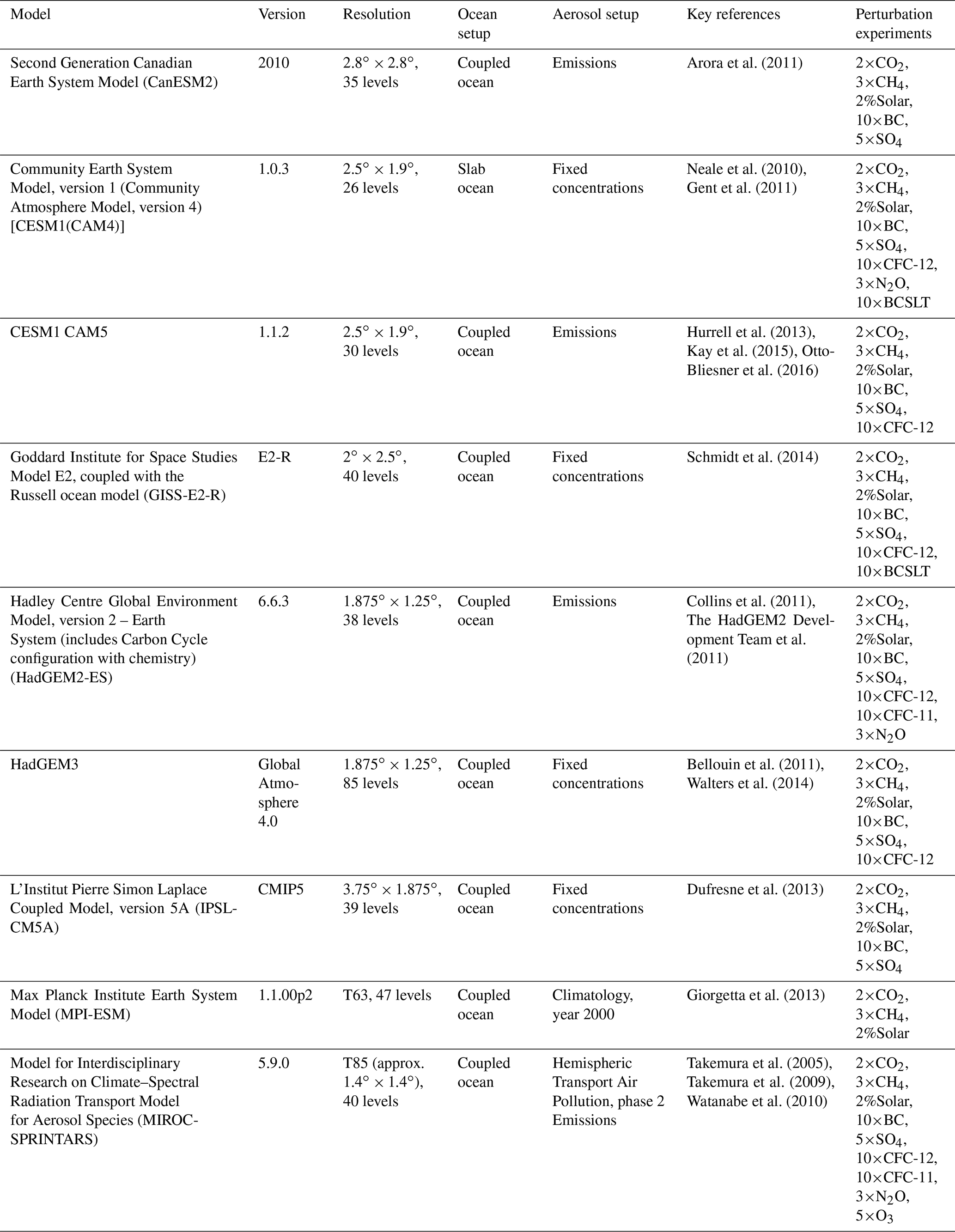
In the perturbation experiments, perturbations on a global scale are applied abruptly at the beginning of the model simulation. The five core experiments include a doubling of CO2 concentration (2×CO2), a tripling of CH4 concentration (3×CH4), a 2 % increase in solar irradiance (2%Solar), an increase in present-day black carbon concentration or emission by a factor of 10 (10×BC), and an increase in present-day SO4 concentration or emission by a factor of 5 (5×SO4). In addition to the five core experiments, a subset of models also performed additional perturbation experiments: an increase in CFC-11 concentration from 535 ppt to 5 ppb (hereafter, 10×CFC-11), an increase in CFC-12 concentration from 653.45 ppt to 5 ppb (hereafter, 10×CFC-12), an increase in N2O concentration from 316 ppb to 1 ppm (hereafter, 3×N2O), an increase in tropospheric O3 concentration used in MacIntosh et al. (2016) by a factor of 5 (5×O3), and an increase in present-day black carbon with a shorter lifetime by a factor of 10 (10×BCSLT). We note that indirect chemical effects are not included in the 3×CH4 experiment. Table 1 provides details about the models and the perturbations each one simulated.
The perturbations in GHGs and solar irradiance are relative to the models' baseline simulations, in which the concentrations of GHGs and solar irradiance are either at present-day levels or preindustrial levels. The perturbations in the aerosols depend on whether it is possible to prescribe aerosol concentrations in the models. For models that are able to prescribe aerosol concentrations, the aerosol perturbations are based on a multi-model mean baseline aerosol concentration in 2000 obtained from the AeroCom Phase II initiative (Myhre et al., 2013a). For those that are only able to produce aerosols through emissions, the perturbation is applied by increasing the emissions by the factors listed above. The 10×BCSLT experiment is performed only by models that are able to prescribe aerosol concentrations.
Each perturbation experiment is performed in two configurations: a fixed sea surface temperatures simulation (“fixed SST”) and a fully coupled (slab ocean for CAM4 only) simulation. The fixed SST simulations use the SST climatology at either the present-day or preindustrial level. The fixed SST simulations are at least 15 years, and the coupled simulations are at least 100 years.
2.2 Fast response and slow response
When available, the SWV mixing ratio is obtained directly from the specific humidity output by each model simulation. For the models that do not output specific humidity (CAM5, GISS-E2-R, and MIROC-SPRINTARS), we calculate specific humidity by multiplying the models' relative humidity by the saturation mixing ratio with respect to ice calculated using model temperature and pressure. Responses of specific humidity and relative humidity in the PDRMIP have been investigated by Hodnebrog et al. (2019), but they focused on water vapor in the troposphere.
We define ΔSWV, the change in the SWV mixing ratio in response to a particular perturbation, to be the difference between SWV in the perturbed coupled run and that in the baseline coupled run. As discussed above, the ΔSWV can then be broken down into the two components: the fast response (ΔSWVfast) and slow response (ΔSWVslow). We compute results in the tropical lower stratosphere (70 hPa, 30∘ N–30∘ S, hereafter, TLS), in the northern hemispheric (NH) lowermost stratosphere (50–90∘ N at 200 hPa, hereafter, NH LMS), and in the southern hemispheric (SH) lowermost stratosphere (50–90∘ S at 200 hPa, hereafter, SH LMS). Most previous studies have focused on the response of water vapor in the TLS (e.g., Gettelman et al., 2010; Shu et al., 2011; Smalley et al., 2017). But recent studies report that the climate is most sensitive to changes in water vapor in the LMS (Solomon et al., 2010; Dessler et al., 2013; Banerjee et al., 2019), so we also investigate that region.
We use the fixed SST simulations to get ΔSWVfast, the rapid adjustment in SWV before sea surface temperature changes. ΔSWVfast is the difference between the SWV mixing ratio averaged over the last 10 years in the fixed SST run with the forcing perturbation and the SWV mixing ratio averaged over the last 10 years in the fixed SST baseline simulation. The fixed SST runs have some warming of the land surface, meaning that our fast response includes a contribution from a warming land surface. We expect this will have a small impact on our results, but it remains one of the uncertainties in our analysis.
We calculate ΔSWVslow as ΔSWV minus ΔSWVfast. To estimate the time series of ΔSWVslow, we use annual mean ΔSWV time series over the entire coupled run period (at least 100 years) minus the 10-year average ΔSWVfast. To estimate equilibrium ΔSWVslow, we use a regression method similar to the methodology introduced by Gregory et al. (2004). The basic concept is that we regress the annual mean global average net downward radiative flux (R) at the top of the atmosphere (TOA) against the annual mean ΔSWV averaged at TLS, NH LMS, or SH LMS. The equilibrium ΔSWV is where the linear fit intercepts at R=0. Then we simply subtract ΔSWVfast from the equilibrium ΔSWV to estimate equilibrium ΔSWVslow.
These regressions can be very noisy and yield highly uncertain parameters, particularly for perturbations with relatively small amounts of radiative forcing and warming. To account for this, we first fit the R and ΔSWV time series using an exponential function () and then do the regression using the fitted time series. For fully coupled models, we constrain τ1 to be within the range of 4±2 years and τ2 to be within the range of 250±70 years; for CAM4, in which the atmosphere is coupled to a slab ocean, we constrain τ1 to be within the range of 4±2 years. We then compute the best fit of all parameters. The ranges for the time constants are based on previous estimations of climate system timescales (Geoffroy et al., 2013). We estimate the ΔSWV intercept at R=0 by regressing the fitted R and ΔSWV data over the last 30 years, since the relation between R and ΔSWV is not necessarily linear over the entire 100-year period. The slow and fast responses of other variables, such as global average surface temperatures and cold-point temperatures, are computed using the same method.
We tested this method in a climate model that nearly reaches the equilibrium climate state. We analyzed runs of the fully coupled Max Planck Institute Earth System Model version 1.1 (MPI-ESM1.1) (Maher et al., 2019), which has a transient climate response and an effective climate sensitivity near the middle of the CMIP5 ensemble range (Adams and Dessler, 2019; Dessler, 2020). It includes a 2000-year preindustrial control run and a 2614-year abruptly quadrupled CO2 run. The values of ΔSWV averaged over the last 30 years of the 4×CO2 run relative to the control run are 4.60 ppmv in the TLS, 22.40 ppmv in the NH LMS, and 9.69 ppmv in the SH LMS. We expect this to be close to equilibrium ΔSWV because the trend in global average surface temperature over the last 500 years of the 4×CO2 run is 0.02 K per century. We use the regression method to estimate the equilibrium ΔSWV using MPI-ESM1.1 water vapor mixing ratio time series over the first 100 years and obtain estimates of 4.38 ppmv in the TLS, 20.01 ppmv in the NH LMS, and 9.07 ppmv in the SH LMS; these yield differences of 0.22 ppmv in the TLS, 2.39 ppmv in the NH LMS, and 0.62 ppmv in the SH LMS. Thus, our method underestimates the true equilibrium value by 5 % in the TLS, 11 % in the NH LMS, and 6 % in the SH LMS.
Uncertainty for slow and fast responses of different quantities shown in this paper is obtained from Monte Carlo samples as follows: for each perturbation, we randomly sample with replacement 100 000 times for each model that performed that perturbation and from these samples compute the 2.5–97.5 percentiles.
3.1 The slow stratospheric water vapor response
We show equilibrium ΔSWVslow and its percentage contribution to the total equilibrium ΔSWV in Fig. 1. We show results in the TLS (Fig. 1a and d), in the NH LMS (Fig. 1b and e), and the SH LMS (Fig. 1c and f). In evaluating the absolute magnitude of ΔSWVslow in the first column of Fig. 1, we normalize the equilibrium ΔSWVslow using effective radiative forcing (ERF) so that differences in the magnitude of the forcing do not confound our results.
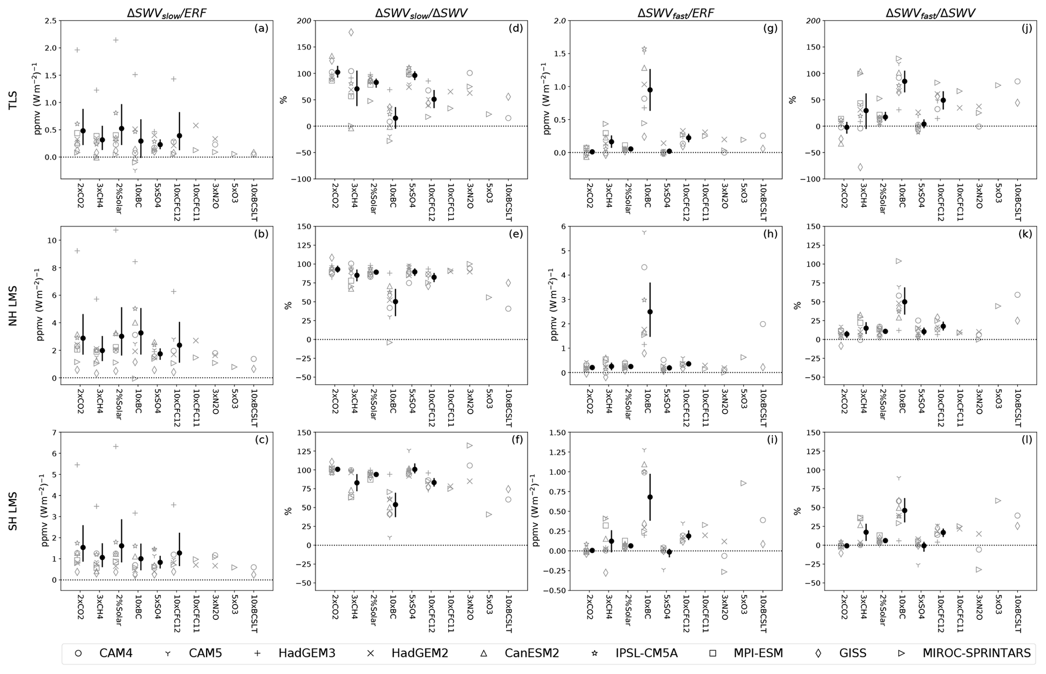
Figure 1(a–c) Equilibrium ΔSWVslow normalized by ERF (ppmv (W m−2)−1) in TLS (70 hPa, 30∘ N–30∘ S), NH LMS (200 hPa, 50–90∘ N), and SH LMS (200 hPa, 50–90∘ S). (d–f) Contribution (%) of equilibrium ΔSWVslow to total equilibrium ΔSWV. (g–i) ΔSWVfast normalized by ERF (ppmv (W m−2)−1). (j–l) Contribution (%) of ΔSWVfast to total equilibrium ΔSWV. The marker shapes indicate results from different models. For perturbations that are performed by more than three models, the solid circles and error bars for each perturbation plotted in solid black are the multi-model mean and 2.5–97.5 percentiles of the model samples. Note that in the second and fourth columns, we took out models with extremely small ΔSWV magnitudes that yield extremely large ΔSWVslow ∕ ΔSWV and ΔSWVfast ∕ ΔSWV ratios.
ERF values used in the construction of Fig. 1 are plotted in Fig. 2a; they are calculated as the difference in net radiation at the top of the atmosphere (TOA) averaged over the last 10 years between the fixed SST perturbed and baseline simulation. Previous studies have computed the ERF in the PDRMIP using various methods (Richardson et al., 2019; Tang et al., 2019). The ERF calculation in our paper uses the same method as the ERFsst in Richardson et al. (2019). We directly compared our ERF with the ERFsst listed in Richardson et al. (2019), which shows good agreement and can be found in the Supplement (Table S3). The equilibrium global averaged surface temperature changes (ΔTs), estimated using the regression method described in Sect. 2.2 and normalized by ERF, are plotted in Fig. 2b. The multi-model mean ΔTs ∕ ERF shows general agreement across different perturbations. This quantity is the inverse of the feedback parameter λ (e.g., Dessler and Zelinka, 2015), so Fig. 2b implies that the climate sensitivity to these different perturbations is similar, which also agrees with Richardson et al. (2019). We list the ERF and ΔTs quantities for each model and perturbation in Table S1.
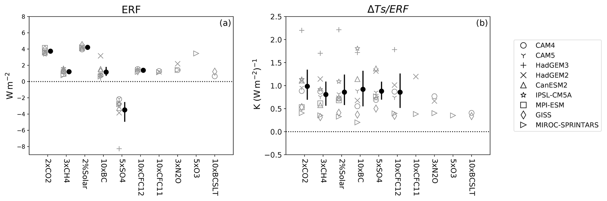
Figure 2(a) Global average ERF (W m−2) at the top of the atmosphere. (b) Global averaged surface temperature change per unit ERF (K (W m−2)−1). The marker shapes indicate results from different models. For perturbations that are performed by more than three models, the solid circles and error bars for each perturbation plotted in solid black are the multi-model mean and 2.5–97.5 percentiles of the model samples.
In each region, the magnitude of multi-model mean ΔSWVslow ∕ ERF shows general agreement for different perturbations. The magnitudes of ΔSWVslow ∕ ERF in the LMS are larger than those in the TLS (Fig. 1b–c). This is consistent with previous studies, which showed that the long-term trend in SWV over the century in climate models is largest near the LMS tropopause (Dessler et al., 2013; Huang et al., 2016; Banerjee et al., 2019). This reflects different transport pathways into the LMS, including downward transport by the Brewer–Dobson circulation, quasi-horizontal isentropic mixing from the tropical troposphere, and convective influence (Dessler et al., 1995; Holton et al., 1995; Plumb, 2002; Gettelman et al., 2011).
In the LMS, the multi-model mean ΔSWVslow ∕ ΔSWV ratio is close to 100 % for many perturbations (Fig. 1e–f). The latitude band (50–90∘) we choose is somewhat arbitrary, so in the Supplement (Fig. S1), we also show ΔSWVslow ∕ ERF and ΔSWVslow ∕ ΔSWV ratios for water vapor averaged at 200 hPa between 30∘ and 50∘ latitudes in the Northern Hemisphere and Southern Hemisphere, respectively, which also show that the ΔSWVslow plays a dominant role and contributes to close to 100 % of the total ΔSWV for most perturbations. In the TLS, the multi-model mean ΔSWVslow ∕ ΔSWV ratio is generally above 50 %, with a few exceptions. We will discuss this in detail in Sect. 3.3.
We note that inter-model variability in ΔSWVslow ∕ ERF and ΔSWVslow is generally consistent for different perturbations. For example, HadGEM3 produces larger responses than the rest of the models for most perturbations (Fig. 1a–c, Table S1). GISS-E2-R and MIROC-SPRINTARS have ΔSWVslow ∕ ERF and ΔSWVslow values generally below the rest of the models (Fig. 1a–c, Table S1). We have not further investigated the causes of these differences among models; this clearly warrants further investigation.
We also note that CAM5, CanESM2, and MIROC-SPRINTARS produce negative TLS ΔSWVslow ∕ ERF for 10×BC. These negative values are partly contributed by artifacts of the method we use to estimate equilibrium ΔSWVslow, which is the residual of the total equilibrium ΔSWV minus ΔSWVfast. When differencing two numbers with similar magnitudes, the residual may be quite uncertain. So, the negative values here do not necessarily mean that a BC-induced surface warming results in a negative SWV slow response. The direct regression between ΔSWVslow and surface temperature change described in the next section more accurately describes the relationship for these cases.
3.2 The slow stratospheric water vapor response and the surface temperature change
Our results show that, in most climate perturbations analyzed in this study, the equilibrium response of water vapor in both the TLS and the LMS is dominated by ΔSWVslow, which is the component mediated by sea surface temperature change. To directly quantify how SWV responds to surface temperature across a range of different climate change mechanisms, we linearly regress the time series of annual mean ΔSWVslow over the entire period of the coupled simulations (at least 100 years) against the time series of annual mean global averaged surface temperature change (ΔTs). We do this regression for each model and perturbation separately. This is similar to the analysis of Banerjee et al. (2019), who did this for quadrupled CO2 perturbation, but we do this for multiple perturbations.
The scatter plot for each perturbation and model is shown in the Supplement (Figs. S3–S5). For most perturbations and models, the ΔSWVslow time series in both the TLS and the LMS is positively correlated with the ΔTs time series, supporting the hypothesis that the surface temperature change contributes to the long-term trend in SWV for most cases.
Figure 3 shows the slopes of the regression for all perturbations and models. The corresponding slope values are listed in Table S4. We also list slopes in the unit of percent per Kelvin (% K−1) in Table S5. The uncertainty of the slopes is obtained from Monte Carlo samples: for each model and perturbation, we first randomly sample the slope 100 000 times, assuming a Gaussian distribution. Then, for each perturbation, we sample from the slope distributions with replacement 100 000 times for each model that performed that perturbation and from these samples compute the 2.5–97.5 percentiles.
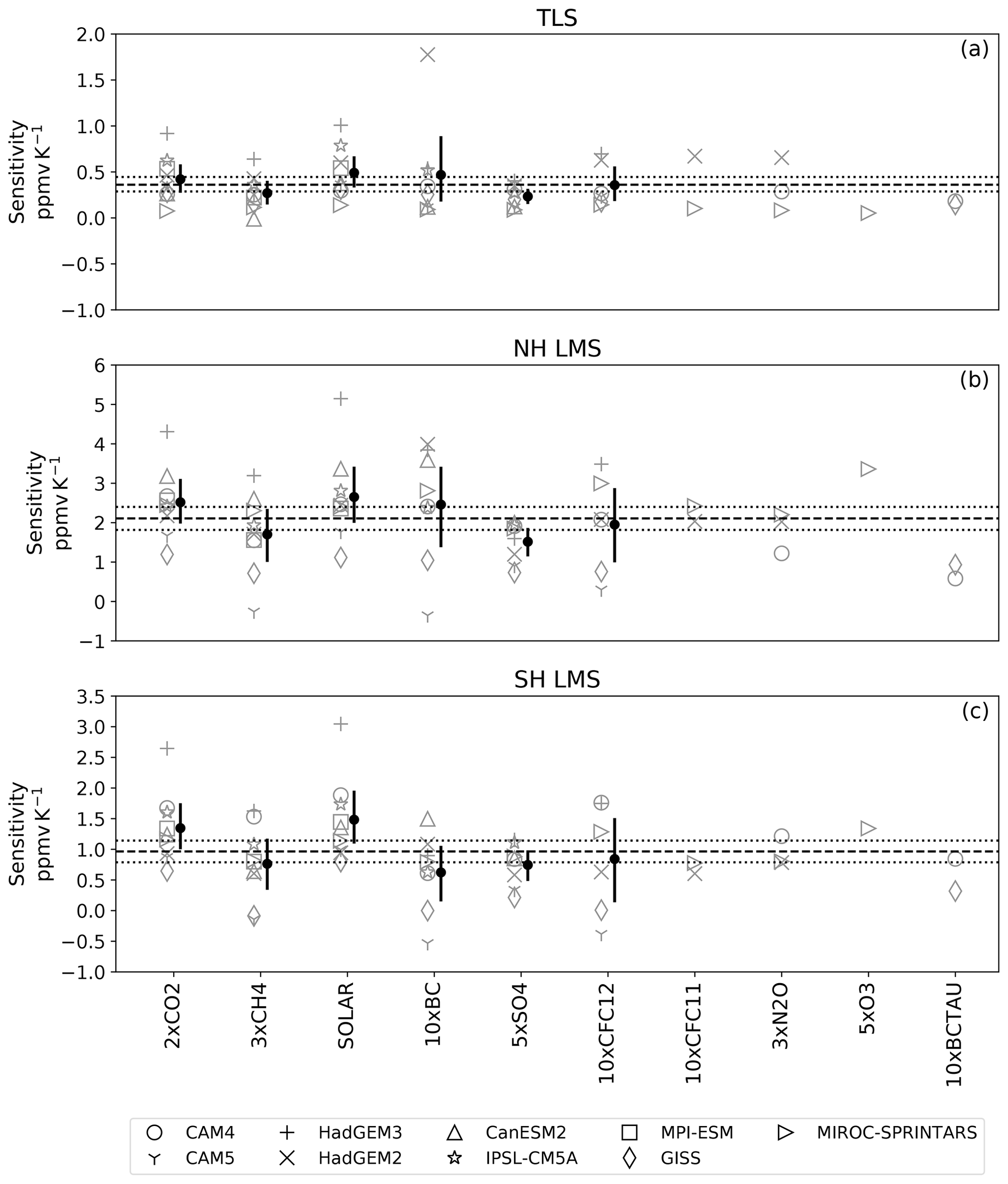
Figure 3Slopes (ppmv K−1) from the linear regression between annual mean ΔSWVslow time series and annual mean ΔTs time series. The marker shapes indicate results from different models. For perturbations that are performed by more than three models, the solid circles and error bars for each perturbation plotted in solid black are the multi-model mean and 2.5–97.5 percentiles of the model samples. The horizontal dashed line is the multi-model mean of all slopes, and the horizontal dotted lines are 2.5–97.5 percentiles of the model samples.
In both the TLS and LMS, the slopes from different perturbations show general agreement (Fig. 3); this is also true for water vapor averaged at 200 hPa between 30∘ and 50∘ latitudes in the Northern Hemisphere and Southern Hemisphere (Fig. S2). In the TLS, the multi-model and multi-perturbation average slope is 0.35 ppmv K−1, with a 95 % confidence interval of 0.28–0.44 ppmv K−1 (Fig. 3a). The LMS ΔSWVslow time series has stronger correlations with the ΔTs time series (Figs. S3–S5) and produces larger sensitivities (Fig. 3b–c). Specifically, the multi-model and multi-perturbation mean slope is 2.1 ppmv K−1 in the Northern Hemisphere and 0.97 ppmv K−1 in the Southern Hemisphere, with 95 % confidence intervals of 1.82–2.39 ppmv K−1 and 0.79–1.15 ppmv K−1, respectively. Our results are similar to those of Dessler et al. (2013) and Smalley et al. (2017) despite the fact that they used 500 hPa temperature as their regressor.
We show that the relation between ΔSWVslow and ΔTs time series can be extended to the entire stratosphere (Fig. 4a). We regridded the zonal mean ΔSWVslow from all models and perturbations onto the same pressure–latitude grid (10 hPa above 100 hPa and 50 hPa below 100 hPa, 4∘ latitude) and regressed the ΔSWVslow time series at each grid point against global average ΔTs time series. The multi-model and multi-perturbation average slope of the linear fit at each grid point is shown in Fig. 4a (figures for each individual perturbation are shown in Fig. S6). Since the vertical gradient of water vapor is large, we plot the percentage change in the mixing ratio per Kelvin relative to the baseline. Lapse rate tropopause, the lowest level where the lapse rate decreases to 2 K km−1, also plotted, is obtained using the atmospheric temperatures from the baseline coupled run and multi-model mean.
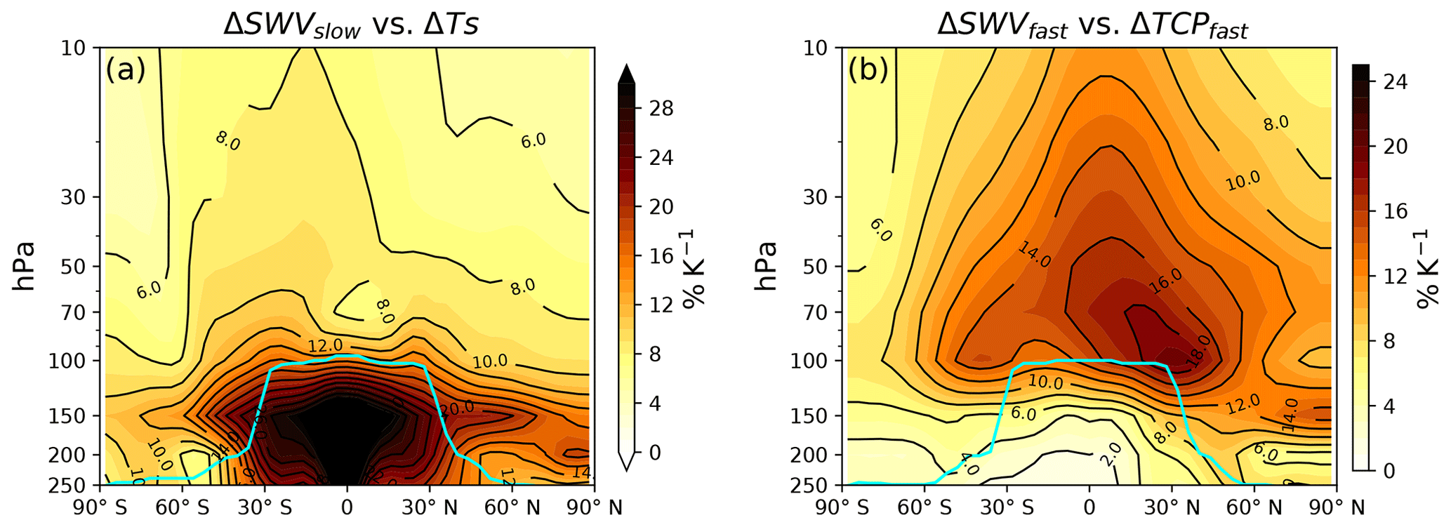
Figure 4(a) Multi-model and multi-perturbation mean slope (% K−1) from the regression between annual mean time series of ΔSWVslow (at each latitude grid point and pressure level) and annual mean time series of global average ΔTs. (b) Slope (% K−1) from the regression between ΔSWVfast (ppmv) (at each latitude grid point and pressure level) and ΔTCPfast (K). The solid cyan line is the multi-model mean lapse rate tropopause derived from the baseline simulations.
We clearly see the larger sensitivity of ΔSWVslow to ΔTs in the LMS than in the overworld. In the LMS, the slope has a hemispheric asymmetry, with larger values in the Northern Hemisphere. This is consistent with previous studies, which showed that isentropic transport brings more tropospheric water vapor to the NH than the SH (Pan et al., 1997, 2000; Dethof et al., 1999, 2000; Ploeger et al., 2013). In addition, convective moistening may be more important to the NH due to more land in the Northern Hemisphere and, consequently, more convection (Dessler and Sherwood, 2004; Smith et al., 2017; Ueyama et al., 2018; Wang et al., 2019). We also see large responses in the tropical upper troposphere, which is the main part of the tropospheric water vapor feedback. The sensitivity declines as one ascends through the TTL. Once above the TTL, the sensitivity in the overworld is relatively uniform with altitude.
3.3 The fast stratospheric water vapor response
Figure 1 also shows the ΔSWVfast normalized by the ERF (Fig. 1g–i) and its contribution to total equilibrium ΔSWV (Fig. 1j–l). As discussed previously, ΔSWVfast is the rapid adjustment in SWV before the sea surface temperatures respond. For most perturbations, especially in the LMS, ΔSWVfast ∕ ERF is smaller than ΔSWVslow ∕ ERF, with a magnitude of a few tenths of a part per million by volume per watt per square meter (ppmv (W m−2)−1).
For 2×CO2, the near-zero TLS ΔSWVfast ∕ ERF is the result of cancellation between cooling by a strengthening Brewer–Dobson circulation and increased local radiative heating (Lin et al., 2017). Some other GHG forcing agents, however, produce larger TLS ΔSWVfast ∕ ERF and contributions in the TLS. For both 10×CFC-12 and 10×CFC-11 the multi-model mean ΔSWVfast contributes about half of the total ΔSWV (Fig. 1j). This is a consequence of halocarbons producing more TTL warming per watt per square meter (W m−2) by efficiently absorbing upwelling longwave radiation from the troposphere in the atmospheric window (Forster et al., 1997; Jain et al., 2000; Forster and Joshi, 2005). Figure 5 shows the fast temperature response per unit ERF due to different perturbations, and it shows heating in the TTL for both 10×CFC-12 and 10×CFC-11.

Figure 5Profiles of fast temperature response normalized by ERF (K (W m−2)−1) between 200 and 40 hPa, averaged over 30∘ N–30∘ S. The color coding indicates results from different perturbations. Each profile is the multi-model mean.
The 3×CH4 also includes some models that produce large TLS ΔSWVfast ∕ ERF magnitudes. This is likely due to TTL heating (Fig. 5) by CH4 shortwave absorption, which is explicitly treated in some models, including CAM5, CanESM2, MPI-ESM, and MIROC-SPRINTARS (Smith et al., 2018). These models are also the ones that produce the largest TLS ΔSWVfast contributions (Fig. 1g and j).
Increases in tropospheric O3 (in the 5×O3 experiment) reduce the upwelling longwave radiation, which cools the stratosphere (Ramaswamy and Bowen, 1994; Berntsen et al., 1997; Forster et al., 1997). The longwave radiation absorbed heats the TTL region (Fig. 5), resulting in larger TLS ΔSWVfast ∕ ERF magnitude than ΔSWVslow ∕ ERF and larger contributions to total equilibrium ΔSWV (77 %) (Fig. 1g and j). There is also heating in the LMS, resulting in larger LMS ΔSWVfast ∕ ERF magnitude than ΔSWVslow ∕ ERF (Fig. 1h–i and k–l). We note that our conclusion on 5×O3 is based on only one model, MIROC-SPRINTARS.
ΔSWVfast from 10×BC dominates total equilibrium ΔSWV in the TLS, with a multi-model mean contribution of 84 %. The magnitude of the multi-model mean ΔSWVfast ∕ ERF from 10×BC is also larger than any other perturbations in each region. This occurs because the 10×BC strongly absorbs shortwave radiation, causing large heating of the tropopause region in both the tropics and extratropics. Figure 5 shows that the 10×BC gives by far the most warming per unit ERF, which is consistent with the vertical profile of fast temperature response shown in Stjern et al. (2017).
The 10×BC ΔSWVfast ∕ ERF in the NH and SH LMS contributes about 50 % of the total equilibrium ΔSWV, with smaller magnitudes in the Southern Hemisphere (Fig. 1h–i and k–l). This is because the total amount of black carbon is smaller in the Southern Hemisphere (Myhre et al., 2017), since black carbon is a combustion product and is predominantly emitted over the NH continents (Ramanathan and Carmichael, 2008). The 10×BCSLT ΔSWVfast also contributes about 50 % of the total 10×BCSLT ΔSWV. The 10×BCSLT does not produce as strong a ΔSWVfast ∕ ERF as 10×BC, since the reduction in BC lifetime leads to less BC in the TTL and therefore less heating per unit ERF.
We quantify control of TLS ΔSWVfast by the fast TTL temperature adjustments across a range of different climate perturbations by regressing the TLS ΔSWVfast against the fast response of the cold-point temperature (ΔTCPfast). To estimate ΔTCPfast in the models, we first find the minimum temperature in the profile at each grid point in the fixed SST runs (no interpolation is done; we simply find the minimum temperature on the output model levels). These minimum temperatures are then averaged between 30∘ N and 30∘ S to yield TCPfast in each run. ΔTCPfast is the difference between TCPfast in the perturbed model run and that in the baseline runs.
We find that TLS ΔSWVfast is strongly correlated with ΔTCPfast across all perturbations and models (Fig. 6a), with a slope of 0.52 ppmv K−1 and a 95 % confidence interval of 0.43 to 0.61 ppmv K−1. Randel and Park (2019) pointed out that the slope from the Clausius–Clapeyron relationship evaluated near the tropical tropopause is close to this value, about 0.5 ppmv K−1. We also tested the relationship between TLS ΔSWVslow and the slow response of the cold-point temperature (ΔTCPslow) across all perturbations and models, yielding a slope of 0.72 ppmv K−1. However, for the slow response, correlation does not necessarily prove causality, since Dessler et al. (2016) showed that, in two climate models at least, a significant fraction of the long-term trend was due to increases in convective moistening, which bypasses the TTL cool trap. Therefore, this relationship for the slow response could arise from either TCP control, a process that correlates with it, such as deep convective injection of ice, or some combination.
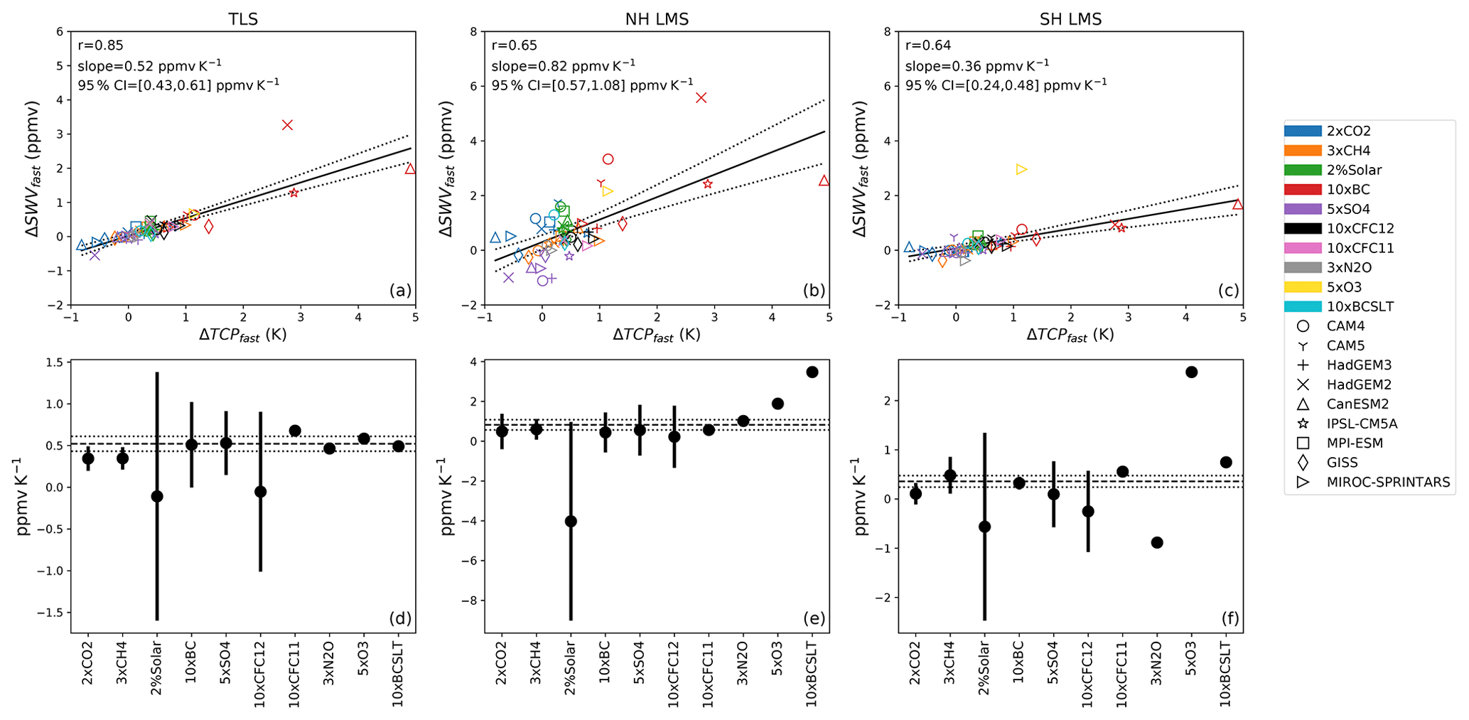
Figure 6(a–c) Linear regression between ΔSWVfast (ppmv) and ΔTCPfast (K) from all models and perturbations. The color coding indicates different perturbations, while the marker shapes indicate results from different models. The black solid line is the linear fit of the regression. The black dotted lines indicate the linear fits within the 95 % confidence interval, estimated using a t test. (d–f) Slopes and their 95 % confidence intervals (for perturbations that are performed by more than three models) obtained from linear regression between ΔSWVfast (ppmv) and ΔTCPfast (K) for each individual perturbation. The black dashed lines and dotted lines are the slopes and their 95 % confidence intervals of the regressions in (a)–(c).
We also separately plot the slopes between ΔSWVfast and ΔTCPfast for each perturbation (Fig. 6d–f). For the perturbations that have more than five participating models, including 2×CO2, 3×CH4, 2%Solar, 10×BC, 5×SO4, and 10×CFC-12, we calculate the linear regression between ΔSWVfast and ΔTCPfast from the models and show the slopes and 95 % confidence intervals. For the perturbations that have fewer participating models, including 10×CFC11, 3×N2O, 5×O3, and 10×BCSLT, we plot the ratio ΔSWVfast ∕ ΔTCPfast and show only the multi-model mean. The slopes produced by different perturbations show general agreement (Fig. 6d). The larger uncertainty in the slopes produced by 2%Solar and 10×CFC-12 occurs because both the ΔTCPfast and ΔSWVfast produced by different models are similar, and therefore the slope of the linear regression is uncertain. Overall, we find that the fast response of TTL temperature is a good predictor for the TLS ΔSWVfast across a range of different climate mechanisms and across multiple models.
For the LMS ΔSWVfast, the ΔTCPfast does not show a control as strong as that in the TLS (Fig. 6b–c) due to the fact that TTL temperatures are only one factor that influences the LMS. In addition, the regression between ΔSWVfast and ΔTCPfast across all perturbations at each grid point in the pressure–latitude domain shows that the slope (% K−1) follows the transport pattern of the Brewer–Dobson circulation (BDC) (Fig. 4b). The slope is large in the tropical overworld stratosphere and becomes weaker as one moves poleward and downward in the extratropics below 150 hPa. The value is lower in the LMS, again consistent with the fact that water vapor in the LMS is controlled by several processes, not just TTL cold-point temperature. Clearly, more work on this is warranted.
Given the importance of SWV change, we now ask whether our results can help us understand historical variations in TLS ΔSWV over 1980–2010 (Fig. 7). To do this, we estimate historical values of ΔSWVslow and ΔSWVfast based on the PDRMIP results, historical surface temperature change, and historical radiative forcing. For the slow component (blue in Fig. 7a), we multiply 0.35 ppmv K−1, the multi-model multi-perturbation mean sensitivity of the PDRMIP TLS ΔSWVslow to ΔTs, by the historical surface temperature change over 1980–2010. For the fast component (orange in Fig. 7a), we multiply the multi-model mean PDRMIP TLS ΔSWVfast ∕ ERF value for each perturbation by the corresponding historical radiative forcing and then sum it up. We also show the fast component of the historical ΔSWV contributed by each historical forcing agent in Fig. 7b. This is similar to the analysis done by Hodnebrog et al. (2019) in their Fig. 6, where they used this method to estimate the historical water vapor lifetime change based on the PDRMIP results.
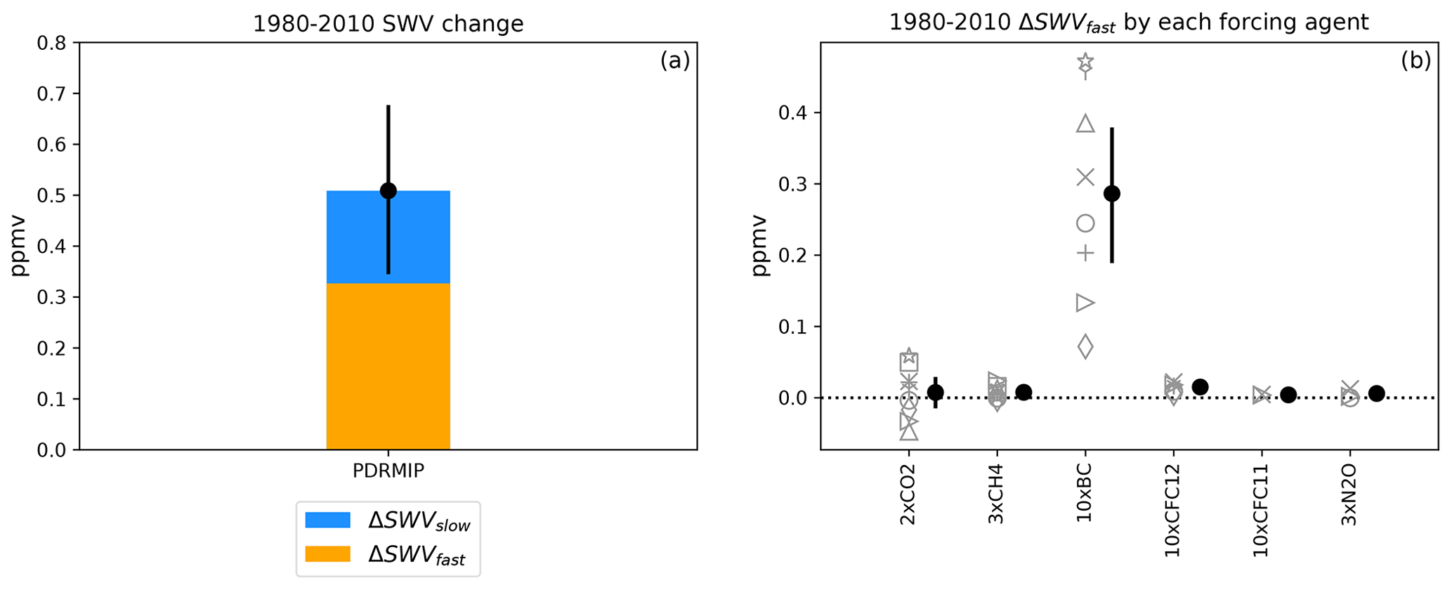
Figure 7(a) TLS (30∘ S–30∘ N, 70 hPa) SWV change over 1980–2010 estimated using PDRMIP results. Blue indicates the component contributed by the slow response, while orange indicates the component contributed by the fast response. (b) The fast component of the PDRMIP-estimated 1980–2010 SWV change contributed by each historical forcing agent. The solid circles are the multi-model mean. The error bars are 2.5–97.5 percentiles of the model samples; in (b) they are shown for perturbations that are performed by more than three models.
The historical surface temperature change and radiative forcing data used in this analysis are listed in Table 2. The historical radiative forcing we use here is defined as the change in net downward radiative flux at the tropopause after adjustments in the stratospheric temperatures, while the surface and troposphere are held unperturbed (Myhre et al., 2013b). This is different from the ERF we use in the PDRMIP calculations, which introduces uncertainties in the fast component of the historical ΔSWV we estimate based on PDRMIP.
Table 2Historical global average surface temperature change and radiative forcing (RF) by greenhouse gases (GHGs) and halocarbons over 1980–2010. The SWV change over 1980–2010 estimated using PDRMIP results is also listed, including the total SWV change, the slow component, and the fast component. For the fast component of SWV change contributed by each forcing agent, multi-model mean results are listed. The uncertainties are 2.5–97.5 percentiles of the model samples.

a We used NOAA Merged Land Ocean Global Surface Temperature Analysis V5 (Zhang et al., 2020) to compute the global surface temperature change. We use values averaged over 2005–2015 minus those averaged over 1975–1985. We compute the RFs using the formulae listed in Table 3 of Myhre et al. (1998). These formulae were also used to compute RFs of CO2, CH4, and N2O in IPCC reports (Myhre et al., 2013b). Concentrations of GHGs were used to compute RFs. CO2 and CH4 are samples collected in glass flasks at Cold Bay, Alaska, United States (CBA), from the ERSL GML website (Dlugokencky et al., 2020a, b). N2O is from the combined nitrous oxide data from the NOAA/ESRL Global Monitoring Division. For CO2, concentrations averaged over 2005–2015 and averaged over 1978–1985 are used. For CH4, concentrations averaged over 2005–2015 and averaged over 1983–1985 are used. For N2O, concentrations averaged over 2005–2015 and averaged over 1977–1985 are used. e–f Concentrations of CFC-12 and CFC-11 were used to compute RFs. We use CFC-12 and CFC-11 data from combined stations from the NOAA/ESRL Global Monitoring Division. Concentrations averaged over 2005–2015 and averaged over 1977–1985 are used. d We use 0.4 W m−2, the BC RF between 1750 and 2011 reported in IPCC AR5, minus 0.1 W m−2, the BC RF between 1750 and 1993 reported in the 1995 IPCC report (see Table 8.4 of Myhre et al., 2013b).
Figure 7a shows our estimate that climate change over 1980–2010 has increased TLS SWV by 0.51±0.16 ppmv (Fig. 7a); 36 % is due to the slow component, although this is probably an overestimate because our sensitivity value estimated using the PDRMIP results is for the long term. We find that the rest of the ΔSWV, 64 %, is due to the fast component, mainly from black carbon. We have also calculated the SWV sensitivity and SWV fast response over 35–45∘ N between 100 and 80 hPa to estimate the historical 1980–2010 ΔSWV using the same method, which is 0.65±0.20 ppmv. This value shows reasonable agreement with the SWV increase measured by Hurst et al. (2011) of 0.71±0.26 ppmv over Boulder between 16 and 18 km over 1980–2010.
Dessler et al. (2014) and Hegglin et al. (2014) argue that there is not a detectible trend over this period. Such a conclusion is not inconsistent with ours because any actual trend estimate has to contend with short-term interannual variability (i.e., like that from the quasi-biennial oscillation and Brewer–Dobson circulation variability), which can mask a small trend. Our estimate of the trend is based on sensitivity estimated from 100-year run, and therefore short-term interannual variability has a small impact. Given a continuous, reliable, long-term SWV observation record in the future, one will be able to better test the model-predicted values.
For the fast component of the estimated historical ΔSWV, radiative forcing by BC plays the dominant role (Fig. 7b). Uncertainties exist in the historical BC radiative forcing we use in this analysis, which is shown in the IPCC AR5 (Myhre et al., 2013b). In addition, Allen et al. (2019) pointed out that the radiative effect by BC in the PDRMIP is different from that shown in models using observationally constrained aerosol forcing, which may overestimate the heating in the upper troposphere–lower stratosphere region. However, Allen et al. (2019) also noted that uncertainties exist in their observationally constrained aerosol forcing. The uncertainties in the impact of BC forcing on SWV clearly merit more analysis in the future.
It is of great interest for the climate community to understand how SWV changes when the climate changes since SWV plays an important role in the Earth's radiative budget and stratospheric ozone chemistry (Solomon et al., 1986, 2010; Dvortsov and Solomon, 2001; Forster and Shine, 2002). In this study, we investigate the response of stratospheric water vapor (SWV) to a range of different climate forcing mechanisms using a multi-model and multiple-forcing-agent framework. We use output from nine CMIP5 models participating in the PDRMIP. Each model performs a baseline and up to 10 climate perturbation experiments, including 2×CO2, 3×CH4, 2%Solar, 10×BC, 5×SO4, 10×CFC-11, 10×CFC-12, 3×N2O, 5×O3, and 10×BCSLT (Table 1). Each perturbation is performed in two configurations, including fixed SST simulations (at least 15 years) and fully coupled simulations (at least 100 years).
To better understand the SWV response (ΔSWV), we partition it into two parts: the slow response (ΔSWVslow) and the fast response (ΔSWVfast). The ΔSWVfast is the change in response to a perturbation on short timescales before the surface temperature has responded. ΔSWVslow occurs on longer timescales and is coupled to the surface temperature change. Our results show that, for most perturbations, ΔSWV in the tropical lower stratosphere (TLS) and in the lowermost stratosphere (LMS) (200 hPa, 50–90∘ N and 50–90∘ S) is dominated by ΔSWVslow (Fig. 1).
Analysis of ΔSWVslow shows that a warming surface increases SWV (Figs. S3–S5). Furthermore, the response of SWV to the surface temperature change has a similar sensitivity across different climate perturbations in both the overworld stratosphere and the lowermost stratosphere (Figs. 3 and 4a). Specifically, the multi-model and multi-perturbation mean slope is 0.35 ppmv K−1 in the TLS, 2.1 ppmv K−1 in the northern hemispheric (NH) LMS, and 0.97 ppmv K−1 in the southern hemispheric (SH) LMS (Fig. 3).
ΔSWVslow in the LMS is more sensitive to ΔTs than the tropical overworld, reflecting different transport pathways into the LMS compared to the overworld (Dessler et al., 1995; Holton et al., 1995; Plumb, 2002; Gettelman et al., 2011). The ΔSWVslow in the NH LMS is more sensitive than the SH LMS, consistent with hemispheric asymmetries in the isentropic transport and convective moistening reported by previous studies (Pan et al., 1997, 2000; Dethof et al., 1999, 2000; Dessler and Sherwood, 2004; Ploeger et al., 2013; Smith et al., 2017; Ueyama et al., 2018; Wang et al., 2019).
The fast response of SWV from most perturbations is weak compared to the slow response and therefore plays a smaller role in ΔSWV (Fig. 1). In the TLS, for forcing agents that directly heat tropopause levels (Fig. 5), ΔSWVfast makes a larger contribution to ΔSWV. In particular, when the climate is perturbed by 10×BC, the ΔSWVfast dominates the ΔSWVslow and has a larger magnitude than any other perturbed simulations. This occurs because black carbon absorbs shortwave radiation in the atmosphere and directly heats the temperatures at tropopause levels. Other forcing agents also heat the tropopause levels and increase ΔSWVfast through absorption of shortwave radiation or longwave radiation at the atmospheric window range (3×CH4, 5×O3, 10×BCSLT, 10×CFC-12, 10×CFC-11), but these are not as strong as 10×BC.
The TLS ΔSWVfast is controlled by the fast response of the cold-point temperature across different climate change mechanisms (Fig. 6), with a slope of 0.52 ppmv K−1, which is consistent with the Clausius–Clapeyron relationship evaluated near the tropical tropopause (Randel and Park, 2019). Control of the cold-point temperature fast response over ΔSWVfast is stronger in the tropical overworld and becomes weaker at higher latitudes and altitudes below 150 hPa in the LMS (Fig. 4b).
The PDRMIP data are publicly freely available (Samset et al., 2016; Myhre et al., 2017); the data can be accessed at http://cicero.uio.no/en/PDRMIP (CICERO, 2019).
The supplement related to this article is available online at: https://doi.org/10.5194/acp-20-13267-2020-supplement.
XW performed analyses and wrote the paper. AED provided the conceptualization, guidance, and editing.
The authors declare that they have no conflict of interest.
This work was also supported by the National Center for Atmospheric Research, which is a major facility sponsored by the National Science Foundation under cooperative agreement no. 1852977. Any opinions, findings, and conclusions or recommendations expressed in this material do not necessarily reflect the views of the National Science Foundation. We would also like to acknowledge the PDRMIP modeling groups and helpful discussions with Andrew Gettelman and William Randel.
This research has been supported by NASA (grant nos. 80NSSC18K0134 and 80NSSC19K0757).
This paper was edited by Mathias Palm and reviewed by two anonymous referees.
Adams, B. K. and Dessler, A. E.: Estimating Transient Climate Response in a Large-Ensemble Global Climate Model Simulation, Geophys. Res. Lett., 46, 311–317, https://doi.org/10.1029/2018GL080714, 2019.
Allen, R. J., Amiri-Farahani, A., Lamarque, J.-F., Smith, C., Shindell, D., Hassan, T., and Chung, C. E.: Observationally constrained aerosol–cloud semi-direct effects, npj Clim. Atmos. Sci., 2, 16, https://doi.org/10.1038/s41612-019-0073-9, 2019.
Arora, V. K., Scinocca, J. F., Boer, G. J., Christian, J. R., Denman, K. L., Flato, G. M., Kharin, V. V., Lee, W. G., and Merryfield, W. J.: Carbon emission limits required to satisfy future representative concentration pathways of greenhouse gases, Geophys. Res. Lett., 38, L05805, https://doi.org/10.1029/2010GL046270, 2011.
Banerjee, A., Chiodo, G., Previdi, M., Ponater, M., Conley, A. J., and Polvani, L. M.: Stratospheric water vapor: an important climate feedback, Clim. Dynam., 53, 1697–1710, https://doi.org/10.1007/s00382-019-04721-4, 2019.
Bellouin, N., Rae, J., Jones, A., Johnson, C., Haywood, J., and Boucher, O.: Aerosol forcing in the Climate Model Intercomparison Project (CMIP5) simulations by HadGEM2-ES and the role of ammonium nitrate, J. Geophys. Res., 116, D20206, https://doi.org/10.1029/2011JD016074, 2011.
Berntsen, T. K., Isaksen, I. S. A., Myhre, G., Fuglestvedt, J. S., Stordal, F., Larsen, T. A., Freckleton, R. S., and Shine, K. P.: Effects of anthropogenic emissions on tropospheric ozone and its radiative forcing, J. Geophys. Res.-Atmos., 102, 28101–28126, https://doi.org/10.1029/97JD02226, 1997.
Brasseur, G. P. and Solomon, S.: Aeronomy of the Middle Atmosphere, Springer, Dordrecht, the Netherlands, 2005.
CICERO: PDRMIP data, available at: http://cicero.uio.no/en/PDRMIP, last access: 29 August 2019.
Collins, W. J., Bellouin, N., Doutriaux-Boucher, M., Gedney, N., Halloran, P., Hinton, T., Hughes, J., Jones, C. D., Joshi, M., Liddicoat, S., Martin, G., O'Connor, F., Rae, J., Senior, C., Sitch, S., Totterdell, I., Wiltshire, A., and Woodward, S.: Development and evaluation of an Earth-System model – HadGEM2, Geosci. Model Dev., 4, 1051–1075, https://doi.org/10.5194/gmd-4-1051-2011, 2011.
Dessler, A. E.: Potential Problems Measuring Climate Sensitivity from the Historical Record, J. Climate, 33, 2237–2248, https://doi.org/10.1175/JCLI-D-19-0476.1, 2020.
Dessler, A. E. and Sherwood, S. C.: Effect of convection on the summertime extratropical lower stratosphere, J. Geophys. Res.-Atmos., 109, D23301, https://doi.org/10.1029/2004JD005209, 2004.
Dessler, A. E. and Zelinka, M. D.: Climate Feedbacks, in: Encyclopedia of Atmospheric Sciences, Edn. 2, edited by: North, G. R., Pyle, J. A., and Zhang, F., Academic Press, Oxford, United Kingdom, Vol. 2, 18–25, 2015.
Dessler, A. E., Hintsa, E. J., Weinstock, E. M., Anderson, J. G., and Chan, K. R.: Mechanisms controlling water vapor in the lower stratosphere: “A tale of two stratospheres”, J. Geophys. Res., 100, 23167, https://doi.org/10.1029/95JD02455, 1995.
Dessler, A. E., Schoeberl, M. R., Wang, T., Davis, S. M., and Rosenlof, K. H.: Stratospheric water vapor feedback, P. Natl. Acad. Sci. USA, 110, 18087–18091, https://doi.org/10.1073/pnas.1310344110, 2013.
Dessler, A. E., Schoeberl, M. R., Wang, T., Davis, S. M., Rosenlof, K. H., and Vernier, J.-P.: Variations of stratospheric water vapor over the past three decades, J. Geophys. Res.-Atmos., 119, 12588–12598, https://doi.org/10.1002/2014JD021712, 2014.
Dessler, A. E., Ye, H., Wang, T., Schoeberl, M. R., Oman, L. D., Douglass, A. R., Butler, A. H., Rosenlof, K. H., Davis, S. M., and Portmann, R. W.: Transport of ice into the stratosphere and the humidification of the stratosphere over the 21st century, Geophys. Res. Lett., 43, 2323–2329, https://doi.org/10.1002/2016GL067991, 2016.
Dethof, A., O'Neill, A., Slingo, J. M., and Smit, H. G. J.: A mechanism for moistening the lower stratosphere involving the Asian summer monsoon, Q. J. R. Meteor. Soc., 125, 1079–1106, https://doi.org/10.1002/qj.1999.49712555602, 1999.
Dethof, A., O'Neill, A., and Slingo, J.: Quantification of the isentropic mass transport across the dynamical tropopause, J. Geophys. Res.-Atmos., 105, 12279–12293, https://doi.org/10.1029/2000JD900127, 2000.
Dlugokencky, E. J., Mund, J. W., Crotwell, A. M., Crotwell, M. J., and Thoning, K. W.: Atmospheric Carbon Dioxide Dry Air Mole Fractions from the NOAA GML Carbon Cycle Cooperative Global Air Sampling Network, 1968–2019, Version: 2020-07, NOAA ESRL Global Monitoring Laboratory, https://doi.org/10.15138/wkgj-f215, 2020a.
Dlugokencky, E. J., Crotwell, A. M., Mund, J. W., Crotwell, M. J., and Thoning, K. W.: Atmospheric Methane Dry Air Mole Fractions from the NOAA GML Carbon Cycle Cooperative Global Air Sampling Network, 1983–2019, Version: 2020-07, NOAA ESRL Global Monitoring Laboratory, https://doi.org/10.15138/VNCZ-M766, 2020b.
Dufresne, J.-L., Foujols, M.-A., Denvil, S., Caubel, A., Marti, O., Aumont, O., Balkanski, Y., Bekki, S., Bellenger, H., Benshila, R., Bony, S., Bopp, L., Braconnot, P., Brockmann, P., Cadule, P., Cheruy, F., Codron, F., Cozic, A., Cugnet, D., de Noblet, N., Duvel, J.-P., Ethé, C., Fairhead, L., Fichefet, T., Flavoni, S., Friedlingstein, P., Grandpeix, J.-Y., Guez, L., Guilyardi, E., Hauglustaine, D., Hourdin, F., Idelkadi, A., Ghattas, J., Joussaume, S., Kageyama, M., Krinner, G., Labetoulle, S., Lahellec, A., Lefebvre, M.-P., Lefevre, F., Levy, C., Li, Z. X., Lloyd, J., Lott, F., Madec, G., Mancip, M., Marchand, M., Masson, S., Meurdesoif, Y., Mignot, J., Musat, I., Parouty, S., Polcher, J., Rio, C., Schulz, M., Swingedouw, D., Szopa, S., Talandier, C., Terray, P., Viovy, N., and Vuichard, N.: Climate change projections using the IPSL-CM5 Earth System Model: from CMIP3 to CMIP5, Clim. Dynam., 40, 2123–2165, https://doi.org/10.1007/s00382-012-1636-1, 2013.
Dvortsov, V. L. and Solomon, S.: Response of the stratospheric temperatures and ozone to past and future increases in stratospheric humidity, J. Geophys. Res.-Atmos., 106, 7505–7514, https://doi.org/10.1029/2000JD900637, 2001.
Forster, P. M. D. F. and Joshi, M.: The Role Of Halocarbons In The Climate Change Of The Troposphere And Stratosphere, Climatic Change, 71, 249–266, https://doi.org/10.1007/s10584-005-5955-7, 2005.
Forster, P. M. de F. and Shine, K. P.: Assessing the climate impact of trends in stratospheric water vapor, Geophys. Res. Lett., 29, 10-1–10-4, https://doi.org/10.1029/2001GL013909, 2002.
Forster, P. M. F., Freckleton, R. S., and Shine, K. P.: On aspects of the concept of radiative forcing, Clim. Dynam., 13, 547–560, https://doi.org/10.1007/s003820050182, 1997.
Fueglistaler, S., Dessler, A. E., Dunkerton, T. J., Folkins, I., Fu, Q., and Mote, P. W.: Tropical tropopause layer, Rev. Geophys., 47, 1–31, https://doi.org/10.1029/2008RG000267, 2009.
Gent, P. R., Danabasoglu, G., Donner, L. J., Holland, M. M., Hunke, E. C., Jayne, S. R., Lawrence, D. M., Neale, R. B., Rasch, P. J., Vertenstein, M., Worley, P. H., Yang, Z.-L., and Zhang, M.: The Community Climate System Model Version 4, J. Climate, 24, 4973–4991, https://doi.org/10.1175/2011JCLI4083.1, 2011.
Geoffroy, O., Saint-Martin, D., Olivié, D. J. L., Voldoire, A., Bellon, G., and Tytéca, S.: Transient Climate Response in a Two-Layer Energy-Balance Model. Part I: Analytical Solution and Parameter Calibration Using CMIP5 AOGCM Experiments, J. Climate, 26, 1841–1857, https://doi.org/10.1175/JCLI-D-12-00195.1, 2013.
Gettelman, A., Hegglin, M. I., Son, S.-W., Kim, J., Fujiwara, M., Birner, T., Kremser, S., Rex, M., Añel, J. A., Akiyoshi, H., Austin, J., Bekki, S., Braesike, P., Brühl, C., Butchart, N., Chipperfield, M., Dameris, M., Dhomse, S., Garny, H., Hardiman, S. C., Jöckel, P., Kinnison, D. E., Lamarque, J. F., Mancini, E., Marchand, M., Michou, M., Morgenstern, O., Pawson, S., Pitari, G., Plummer, D., Pyle, J. A., Rozanov, E., Scinocca, J., Shepherd, T. G., Shibata, K., Smale, D., Teyssèdre, H., and Tian, W.: Multimodel assessment of the upper troposphere and lower stratosphere: Tropics and global trends, J. Geophys. Res., 115, D00M08, https://doi.org/10.1029/2009JD013638, 2010.
Gettelman, A., Hoor, P., Pan, L. L., Randel, W. J., Hegglin, M. I., and Birner, T.: THE EXTRATROPICAL UPPER TROPOSPHERE AND LOWER STRATOSPHERE, Rev. Geophys., 49, RG3003, https://doi.org/10.1029/2011RG000355, 2011.
Giorgetta, M. A., Jungclaus, J., Reick, C. H., Legutke, S., Bader, J., Böttinger, M., Brovkin, V., Crueger, T., Esch, M., Fieg, K., Glushak, K., Gayler, V., Haak, H., Hollweg, H.-D., Ilyina, T., Kinne, S., Kornblueh, L., Matei, D., Mauritsen, T., Mikolajewicz, U., Mueller, W., Notz, D., Pithan, F., Raddatz, T., Rast, S., Redler, R., Roeckner, E., Schmidt, H., Schnur, R., Segschneider, J., Six, K. D., Stockhause, M., Timmreck, C., Wegner, J., Widmann, H., Wieners, K.-H., Claussen, M., Marotzke, J., and Stevens, B.: Climate and carbon cycle changes from 1850 to 2100 in MPI-ESM simulations for the Coupled Model Intercomparison Project phase 5, J. Adv. Model. Earth Syst., 5, 572–597, https://doi.org/10.1002/jame.20038, 2013.
Gregory, J. M., Ingram, W. J., Palmer, M. A., Jones, G. S., Stott, P. A., Thorpe, R. B., Lowe, J. A., Johns, T. C., and Williams, K. D.: A new method for diagnosing radiative forcing and climate sensitivity, Geophys. Res. Lett., 31, L03205, https://doi.org/10.1029/2003GL018747, 2004.
Hegglin, M. I., Plummer, D. A., Shepherd, T. G., Scinocca, J. F., Anderson, J., Froidevaux, L., Funke, B., Hurst, D., Rozanov, A., Urban, J., von Clarmann, T., Walker, K. A., Wang, H. J., Tegtmeier, S., and Weigel, K.: Vertical structure of stratospheric water vapour trends derived from merged satellite data, Nat. Geosci., 7, 768–776, https://doi.org/10.1038/ngeo2236, 2014.
Hodnebrog, Ø., Myhre, G., Samset, B. H., Alterskjær, K., Andrews, T., Boucher, O., Faluvegi, G., Fläschner, D., Forster, P. M., Kasoar, M., Kirkevåg, A., Lamarque, J.-F., Olivié, D., Richardson, T. B., Shawki, D., Shindell, D., Shine, K. P., Stier, P., Takemura, T., Voulgarakis, A., and Watson-Parris, D.: Water vapour adjustments and responses differ between climate drivers, Atmos. Chem. Phys., 19, 12887–12899, https://doi.org/10.5194/acp-19-12887-2019, 2019.
Holton, J. R., Haynes, P. H., McIntyre, M. E., Douglass, A. R., Rood, R. B., and Pfister, L.: Stratosphere-troposphere exchange, Rev. Geophys., 33, 403, https://doi.org/10.1029/95RG02097, 1995.
Hoskins, B. J.: Towards a PV-θ view of the general circulation, Tellus A, 43, 27–36, https://doi.org/10.3402/tellusa.v43i4.11936, 1991.
Huang, Y., Zhang, M., Xia, Y., Hu, Y., and Son, S.-W.: Is there a stratospheric radiative feedback in global warming simulations?, Clim. Dynam., 46, 177–186, https://doi.org/10.1007/s00382-015-2577-2, 2016.
Hurrell, J. W., Holland, M. M., Gent, P. R., Ghan, S., Kay, J. E., Kushner, P. J., Lamarque, J.-F., Large, W. G., Lawrence, D., Lindsay, K., Lipscomb, W. H., Long, M. C., Mahowald, N., Marsh, D. R., Neale, R. B., Rasch, P., Vavrus, S., Vertenstein, M., Bader, D., Collins, W. D., Hack, J. J., Kiehl, J., and Marshall, S.: The Community Earth System Model: A Framework for Collaborative Research, B. Am. Meteorol. Soc., 94, 1339–1360, https://doi.org/10.1175/BAMS-D-12-00121.1, 2013.
Hurst, D. F., Oltmans, S. J., Vömel, H., Rosenlof, K. H., Davis, S. M., Ray, E. A., Hall, E. G., and Jordan, A. F.: Stratospheric water vapor trends over Boulder, Colorado: Analysis of the 30 year Boulder record, J. Geophys. Res., 116, D02306, https://doi.org/10.1029/2010JD015065, 2011.
Jain, A. K., Briegleb, B. P., Minschwaner, K., and Wuebbles, D. J.: Radiative forcings and global warming potentials of 39 greenhouse gases, J. Geophys. Res.-Atmos., 105, 20773–20790, https://doi.org/10.1029/2000JD900241, 2000.
Kay, J. E., Deser, C., Phillips, A., Mai, A., Hannay, C., Strand, G., Arblaster, J. M., Bates, S. C., Danabasoglu, G., Edwards, J., Holland, M., Kushner, P., Lamarque, J.-F., Lawrence, D., Lindsay, K., Middleton, A., Munoz, E., Neale, R., Oleson, K., Polvani, L., and Vertenstein, M.: The Community Earth System Model (CESM) Large Ensemble Project: A Community Resource for Studying Climate Change in the Presence of Internal Climate Variability, B. Am. Meteorol. Soc., 96, 1333–1349, https://doi.org/10.1175/BAMS-D-13-00255.1, 2015.
Lin, P., Paynter, D., Ming, Y., and Ramaswamy, V.: Changes of the Tropical Tropopause Layer under Global Warming, J. Climate, 30, 1245–1258, https://doi.org/10.1175/JCLI-D-16-0457.1, 2017.
MacIntosh, C. R., Allan, R. P., Baker, L. H., Bellouin, N., Collins, W., Mousavi, Z., and Shine, K. P.: Contrasting fast precipitation responses to tropospheric and stratospheric ozone forcing, Geophys. Res. Lett., 43, 1263–1271, https://doi.org/10.1002/2015GL067231, 2016.
Maher, N., Milinski, S., Suarez-Gutierrez, L., Botzet, M., Dobrynin, M., Kornblueh, L., Kröger, J., Takano, Y., Ghosh, R., Hedemann, C., Li, C., Li, H., Manzini, E., Notz, D., Putrasahan, D., Boysen, L., Claussen, M., Ilyina, T., Olonscheck, D., Raddatz, T., Stevens, B., and Marotzke, J.: The Max Planck Institute Grand Ensemble: Enabling the Exploration of Climate System Variability, J. Adv. Model. Earth Syst., 11, 2050–2069, https://doi.org/10.1029/2019MS001639, 2019.
Mote, P. W., Rosenlof, K. H., McIntyre, M. E., Carr, E. S., Gille, J. C., Holton, J. R., Kinnersley, J. S., Pumphrey, H. C., Russell III, J. M., and Waters, J. W.: An atmospheric tape recorder: The imprint of tropical tropopause temperatures on stratospheric water vapor, J. Geophys. Res., 101, 3989–4006, https://doi.org/10.1029/95JD03422, 1996.
Myhre, G., Highwood, E. J., Shine, K. P., and Stordal, F.: New estimates of radiative forcing due to well mixed greenhouse gases, Geophys. Res. Lett., 25, 2715–2718, https://doi.org/10.1029/98GL01908, 1998.
Myhre, G., Samset, B. H., Schulz, M., Balkanski, Y., Bauer, S., Berntsen, T. K., Bian, H., Bellouin, N., Chin, M., Diehl, T., Easter, R. C., Feichter, J., Ghan, S. J., Hauglustaine, D., Iversen, T., Kinne, S., Kirkevåg, A., Lamarque, J.-F., Lin, G., Liu, X., Lund, M. T., Luo, G., Ma, X., van Noije, T., Penner, J. E., Rasch, P. J., Ruiz, A., Seland, Ø., Skeie, R. B., Stier, P., Takemura, T., Tsigaridis, K., Wang, P., Wang, Z., Xu, L., Yu, H., Yu, F., Yoon, J.-H., Zhang, K., Zhang, H., and Zhou, C.: Radiative forcing of the direct aerosol effect from AeroCom Phase II simulations, Atmos. Chem. Phys., 13, 1853–1877, https://doi.org/10.5194/acp-13-1853-2013, 2013a.
Myhre, G., Shindell, D., Bréon, F.-M., Collins, W., Fuglestvedt, J., Huang, J., Koch, D., Lamarque, J.-F., Lee, D., B., Mendoza, Nakajima, T., Robock, A., Stephens, G., Takemura, T., and Zhang, H.: Anthropogenic and Natural Radiative Forcing, in: Climate Change 2013: The Physical Science Basis, Contribution of Working Group I to the Fifth Assessment Report of the Intergovernmental Panel on Climate Change, edited by: Stocker, T. F., Qin, D., Plattner, G.-K., Tignor, M., Allen, S. K., Boschung, J., Nauels, A., Xia, Y., Bex, V., and Midgley, P. M., 659–740, Cambridge University Press, Cambridge, United Kingdom and New York, NY, USA, https://doi.org/10.1017/CBO9781107415324.018, 2013b.
Myhre, G., Forster, P. M., Samset, B. H., Hodnebrog, Ø., Sillmann, J., Aalbergsjø, S. G., Andrews, T., Boucher, O., Faluvegi, G., Fläschner, D., Iversen, T., Kasoar, M., Kharin, V., Kirkevåg, A., Lamarque, J.-F., Olivié, D., Richardson, T. B., Shindell, D., Shine, K. P., Stjern, C. W., Takemura, T., Voulgarakis, A., and Zwiers, F.: PDRMIP: A Precipitation Driver and Response Model Intercomparison Project – Protocol and Preliminary Results, B. Am. Meteorol. Soc., 98, 1185–1198, https://doi.org/10.1175/BAMS-D-16-0019.1, 2017.
Neale, R. B., Richter, J. H., Conley, A. J., Park, S., Lauritzen, P. H., Gettelman, A., Williamson, D. L., Rasch, P. J., Vavrus, S. J., Taylor, M. A., Collins, W. D., Zhang, M., and Lin, S.: Description of the NCAR Community Atmosphere Model (CAM 4.0), NCAR Technical Note, NCAR/TN-485+STR, Climate And Global Dynamics Division National Center For Atmospheric Research Boulder, Colorado, USA, 224 pp., 2010.
Otto-Bliesner, B. L., Brady, E. C., Fasullo, J., Jahn, A., Landrum, L., Stevenson, S., Rosenbloom, N., Mai, A., and Strand, G.: Climate Variability and Change since 850 CE: An Ensemble Approach with the Community Earth System Model, B. Am. Meteorol. Soc., 97, 735–754, https://doi.org/10.1175/BAMS-D-14-00233.1, 2016.
Pan, L., Solomon, S., Randel, W., Lamarque, J.-F., Hess, P., Gille, J., Chiou, E.-W., and McCormick, M. P.: Hemispheric asymmetries and seasonal variations of the lowermost stratospheric water vapor and ozone derived from SAGE II data, J. Geophys. Res.-Atmos., 102, 28177–28184, https://doi.org/10.1029/97JD02778, 1997.
Pan, L. L., Hintsa, E. J., Stone, E. M., Weinstock, E. M., and Randel, W. J.: The seasonal cycle of water vapor and saturation vapor mixing ratio in the extratropical lowermost stratosphere, J. Geophys. Res.-Atmos., 105, 26519–26530, https://doi.org/10.1029/2000JD900401, 2000.
Ploeger, F., Günther, G., Konopka, P., Fueglistaler, S., Müller, R., Hoppe, C., Kunz, A., Spang, R., Grooß, J.-U., and Riese, M.: Horizontal water vapor transport in the lower stratosphere from subtropics to high latitudes during boreal summer, J. Geophys. Res.-Atmos., 118, 8111–8127, https://doi.org/10.1002/jgrd.50636, 2013.
Plumb, R. A.: Stratospheric Transport, J. Meteorol. Soc. Jpn. Ser. II, 80, 793–809, https://doi.org/10.2151/jmsj.80.793, 2002.
Ramanathan, V. and Carmichael, G.: Global and regional climate changes due to black carbon, Nat. Geosci., 1, 221–227, https://doi.org/10.1038/ngeo156, 2008.
Ramaswamy, V. and Bowen, M. M.: Effect of changes in radiatively active species upon the lower stratospheric temperatures, J. Geophys. Res., 99, 18909, https://doi.org/10.1029/94JD01310, 1994.
Randel, W. and Park, M.: Diagnosing Observed Stratospheric Water Vapor Relationships to the Cold Point Tropical Tropopause, J. Geophys. Res.-Atmos., 124, 7018–7033, https://doi.org/10.1029/2019JD030648, 2019.
Revell, L. E., Stenke, A., Rozanov, E., Ball, W., Lossow, S., and Peter, T.: The role of methane in projections of 21st century stratospheric water vapour, Atmos. Chem. Phys., 16, 13067–13080, https://doi.org/10.5194/acp-16-13067-2016, 2016.
Richardson, T. B., Forster, P. M., Smith, C. J., Maycock, A. C., Wood, T., Andrews, T., Boucher, O., Faluvegi, G., Fläschner, D., Hodnebrog, Ø., Kasoar, M., Kirkevåg, A., Lamarque, J.-F., Mülmenstädt, J., Myhre, G., Olivié, D., Portmann, R. W., Samset, B. H., Shawki, D., Shindell, D., Stier, P., Takemura, T., Voulgarakis, A., and Watson-Parris, D.: Efficacy of Climate Forcings in PDRMIP Models, J. Geophys. Res.-Atmos., 124, 12824–12844, https://doi.org/10.1029/2019JD030581, 2019.
Samset, B. H., Myhre, G., Forster, P. M., Hodnebrog, Ø., Andrews, T., Faluvegi, G., Fläschner, D., Kasoar, M., Kharin, V., Kirkevåg, A., Lamarque, J.-F., Olivié, D., Richardson, T., Shindell, D., Shine, K. P., Takemura, T., and Voulgarakis, A.: Fast and slow precipitation responses to individual climate forcers: A PDRMIP multimodel study, Geophys. Res. Lett., 43, 2782–2791, https://doi.org/10.1002/2016GL068064, 2016.
Schmidt, G. A., Kelley, M., Nazarenko, L., Ruedy, R., Russell, G. L., Aleinov, I., Bauer, M., Bauer, S. E., Bhat, M. K., Bleck, R., Canuto, V., Chen, Y.-H., Cheng, Y., Clune, T. L., Del Genio, A., de Fainchtein, R., Faluvegi, G., Hansen, J. E., Healy, R. J., Kiang, N. Y., Koch, D., Lacis, A. A., LeGrande, A. N., Lerner, J., Lo, K. K., Matthews, E. E., Menon, S., Miller, R. L., Oinas, V., Oloso, A. O., Perlwitz, J. P., Puma, M. J., Putman, W. M., Rind, D., Romanou, A., Sato, M., Shindell, D. T., Sun, S., Syed, R. A., Tausnev, N., Tsigaridis, K., Unger, N., Voulgarakis, A., Yao, M.-S., and Zhang, J.: Configuration and assessment of the GISS ModelE2 contributions to the CMIP5 archive, J. Adv. Model. Earth Syst., 6, 141–184, https://doi.org/10.1002/2013MS000265, 2014.
Sherwood, S. C., Bony, S., Boucher, O., Bretherton, C., Forster, P. M., Gregory, J. M., and Stevens, B.: Adjustments in the Forcing-Feedback Framework for Understanding Climate Change, B. Am. Meteorol. Soc., 96, 217–228, https://doi.org/10.1175/BAMS-D-13-00167.1, 2015.
Shu, J., Tian, W., Austin, J., Chipperfield, M. P., Xie, F., and Wang, W.: Effects of sea surface temperature and greenhouse gas changes on the transport between the stratosphere and troposphere, J. Geophys. Res., 116, D02124, https://doi.org/10.1029/2010JD014520, 2011.
Smalley, K. M., Dessler, A. E., Bekki, S., Deushi, M., Marchand, M., Morgenstern, O., Plummer, D. A., Shibata, K., Yamashita, Y., and Zeng, G.: Contribution of different processes to changes in tropical lower-stratospheric water vapor in chemistry–climate models, Atmos. Chem. Phys., 17, 8031–8044, https://doi.org/10.5194/acp-17-8031-2017, 2017.
Smith, C. J., Kramer, R. J., Myhre, G., Forster, P. M., Soden, B. J., Andrews, T., Boucher, O., Faluvegi, G., Fläschner, D., Hodnebrog, Ø., Kasoar, M., Kharin, V., Kirkevåg, A., Lamarque, J.-F., Mülmenstädt, J., Olivié, D., Richardson, T., Samset, B. H., Shindell, D., Stier, P., Takemura, T., Voulgarakis, A., and Watson-Parris, D.: Understanding Rapid Adjustments to Diverse Forcing Agents, Geophys. Res. Lett., 45, 12023–12031, https://doi.org/10.1029/2018GL079826, 2018.
Smith, J. B., Wilmouth, D. M., Bedka, K. M., Bowman, K. P., Homeyer, C. R., Dykema, J. A., Sargent, M. R., Clapp, C. E., Leroy, S. S., Sayres, D. S., Dean-Day, J. M., Paul Bui, T., and Anderson, J. G.: A case study of convectively sourced water vapor observed in the overworld stratosphere over the United States, J. Geophys. Res.-Atmos., 122, 9529–9554, https://doi.org/10.1002/2017JD026831, 2017.
Solomon, S., Garcia, R. R., Rowland, F. S., and Wuebbles, D. J.: On the depletion of Antarctic ozone, Nature, 321, 755–758, https://doi.org/10.1038/321755a0, 1986.
Solomon, S., Rosenlof, K. H., Portmann, R. W., Daniel, J. S., Davis, S. M., Sanford, T. J., and Plattner, G.-K.: Contributions of Stratospheric Water Vapor to Decadal Changes in the Rate of Global Warming, Science, 327, 1219–1223, https://doi.org/10.1126/science.1182488, 2010.
Stjern, C. W., Samset, B. H., Myhre, G., Forster, P. M., Hodnebrog, Ø., Andrews, T., Boucher, O., Faluvegi, G., Iversen, T., Kasoar, M., Kharin, V., Kirkevåg, A., Lamarque, J.-F., Olivié, D., Richardson, T., Shawki, D., Shindell, D., Smith, C. J., Takemura, T., and Voulgarakis, A.: Rapid Adjustments Cause Weak Surface Temperature Response to Increased Black Carbon Concentrations, J. Geophys. Res.-Atmos., 122, 11462–11481, https://doi.org/10.1002/2017JD027326, 2017.
Takemura, T., Nozawa, T., Emori, S., Nakajima, T. Y., and Nakajima, T.: Simulation of climate response to aerosol direct and indirect effects with aerosol transport-radiation model, J. Geophys. Res., 110, D02202, https://doi.org/10.1029/2004JD005029, 2005.
Takemura, T., Egashira, M., Matsuzawa, K., Ichijo, H., O'ishi, R., and Abe-Ouchi, A.: A simulation of the global distribution and radiative forcing of soil dust aerosols at the Last Glacial Maximum, Atmos. Chem. Phys., 9, 3061–3073, https://doi.org/10.5194/acp-9-3061-2009, 2009.
Tang, T., Shindell, D., Samset, B. H., Boucher, O., Forster, P. M., Hodnebrog, Ø., Myhre, G., Sillmann, J., Voulgarakis, A., Andrews, T., Faluvegi, G., Fläschner, D., Iversen, T., Kasoar, M., Kharin, V., Kirkevåg, A., Lamarque, J.-F., Olivié, D., Richardson, T., Stjern, C. W., and Takemura, T.: Dynamical response of Mediterranean precipitation to greenhouse gases and aerosols, Atmos. Chem. Phys., 18, 8439–8452, https://doi.org/10.5194/acp-18-8439-2018, 2018.
Tang, T., Shindell, D., Faluvegi, G., Myhre, G., Olivié, D., Voulgarakis, A., Kasoar, M., Andrews, T., Boucher, O., Forster, P. M., Hodnebrog, Ø., Iversen, T., Kirkevåg, A., Lamarque, J.-F., Richardson, T., Samset, B. H., Stjern, C. W., Takemura, T., and Smith, C.: Comparison of Effective Radiative Forcing Calculations Using Multiple Methods, Drivers, and Models, J. Geophys. Res.-Atmos., 124, 4382–4394, https://doi.org/10.1029/2018JD030188, 2019.
The HadGEM2 Development Team: G. M. Martin, Bellouin, N., Collins, W. J., Culverwell, I. D., Halloran, P. R., Hardiman, S. C., Hinton, T. J., Jones, C. D., McDonald, R. E., McLaren, A. J., O'Connor, F. M., Roberts, M. J., Rodriguez, J. M., Woodward, S., Best, M. J., Brooks, M. E., Brown, A. R., Butchart, N., Dearden, C., Derbyshire, S. H., Dharssi, I., Doutriaux-Boucher, M., Edwards, J. M., Falloon, P. D., Gedney, N., Gray, L. J., Hewitt, H. T., Hobson, M., Huddleston, M. R., Hughes, J., Ineson, S., Ingram, W. J., James, P. M., Johns, T. C., Johnson, C. E., Jones, A., Jones, C. P., Joshi, M. M., Keen, A. B., Liddicoat, S., Lock, A. P., Maidens, A. V., Manners, J. C., Milton, S. F., Rae, J. G. L., Ridley, J. K., Sellar, A., Senior, C. A., Totterdell, I. J., Verhoef, A., Vidale, P. L., and Wiltshire, A.: The HadGEM2 family of Met Office Unified Model climate configurations, Geosci. Model Dev., 4, 723–757, https://doi.org/10.5194/gmd-4-723-2011, 2011.
Thuburn, J. and Craig, G. C.: On the temperature structure of the tropical substratosphere, J. Geophys. Res., 107, 4017, https://doi.org/10.1029/2001JD000448, 2002.
Ueyama, R., Jensen, E. J., and Pfister, L.: Convective Influence on the Humidity and Clouds in the Tropical Tropopause Layer During Boreal Summer, J. Geophys. Res.-Atmos., 123, 7576–7593, https://doi.org/10.1029/2018JD028674, 2018.
Walters, D. N., Williams, K. D., Boutle, I. A., Bushell, A. C., Edwards, J. M., Field, P. R., Lock, A. P., Morcrette, C. J., Stratton, R. A., Wilkinson, J. M., Willett, M. R., Bellouin, N., Bodas-Salcedo, A., Brooks, M. E., Copsey, D., Earnshaw, P. D., Hardiman, S. C., Harris, C. M., Levine, R. C., MacLachlan, C., Manners, J. C., Martin, G. M., Milton, S. F., Palmer, M. D., Roberts, M. J., Rodríguez, J. M., Tennant, W. J., and Vidale, P. L.: The Met Office Unified Model Global Atmosphere 4.0 and JULES Global Land 4.0 configurations, Geosci. Model Dev., 7, 361–386, https://doi.org/10.5194/gmd-7-361-2014, 2014.
Wang, X., Dessler, A. E., Schoeberl, M. R., Yu, W., and Wang, T.: Impact of convectively lofted ice on the seasonal cycle of water vapor in the tropical tropopause layer, Atmos. Chem. Phys., 19, 14621–14636, https://doi.org/10.5194/acp-19-14621-2019, 2019.
Watanabe, M., Suzuki, T., O'ishi, R., Komuro, Y., Watanabe, S., Emori, S., Takemura, T., Chikira, M., Ogura, T., Sekiguchi, M., Takata, K., Yamazaki, D., Yokohata, T., Nozawa, T., Hasumi, H., Tatebe, H., and Kimoto, M.: Improved Climate Simulation by MIROC5: Mean States, Variability, and Climate Sensitivity, J. Climate, 23, 6312–6335, https://doi.org/10.1175/2010JCLI3679.1, 2010.
Xia, Y., Huang, Y., Hu, Y., and Yang, J.: Impacts of tropical tropopause warming on the stratospheric water vapor, Clim. Dynam., 53, 3409–3418, https://doi.org/10.1007/s00382-019-04714-3, 2019.
Zelinka, M. D., Myers, T. A., McCoy, D. T., Po-Chedley, S., Caldwell, P. M., Ceppi, P., Klein, S. A., and Taylor, K. E.: Causes of higher climate sensitivity in CMIP6 models, Geophys. Res. Lett., 47, e2019GL085782, https://doi.org/10.1029/2019GL085782, 2020.
Zhang, H.-M., Huang, B., Lawrimore, J., Menne, M., and Smith, T. M.: NOAA Global Surface Temperature Dataset (NOAAGlobalTemp), Version 5.0, NOAA National Centers for Environmental Information, https://doi.org/10.7289/V5FN144H, 2019.