On the role of trend and variability in the hydroxyl radical (OH) in the global methane budget

Decadal trends and interannual variations in the hydroxyl radical (OH), while poorly constrained at present, are critical for understanding the observed evolution of atmospheric methane (CH₄). Through analyzing the OH fields simulated by the model ensemble of the Chemistry–Climate Model Initiative (CCMI), we find (1) the negative OH anomalies during the El Niño years mainly corresponding to the enhanced carbon monoxide (CO) emissions from biomass burning and (2) a positive OH trend during 1980–2010 dominated by the elevated primary production and the reduced loss of OH due to decreasing CO after 2000. Both two-box model inversions and variational 4D inversions suggest that ignoring the negative anomaly of OH during the El Niño years leads to a large overestimation of the increase in global CH₄ emissions by up to 10 ± 3 Tg yr⁻¹ to match the observed CH₄ increase over these years. Not accounting for the increasing OH trends given by the CCMI models leads to an underestimation of the CH₄ emission increase by 23 ± 9 Tg yr⁻¹ from 1986 to 2010. The variational-inversion-estimated CH₄ emissions show that the tropical regions contribute most to the uncertainties related to OH. This study highlights the significant impact of climate and chemical feedbacks related to OH on the top-down estimates of the global CH₄ budget.

1 Introduction

Methane (CH₄) in the Earth's atmosphere is a major anthropogenic greenhouse gas that has resulted in a 0.62 W m⁻² additional radiative forcing from 1750 to 2011 (Etminan et al., 2016). The tropospheric CH₄ mixing ratio has more than doubled between the preindustrial period and the present day, mainly attributed to increasing anthropogenic CH₄ emissions (Etheridge et al., 1998; Turner et al., 2019). Although the centennial and interdecadal trends and the drivers of CH₄ growth are fairly clear, it is still challenging to understand the trends and the associated interannual variations on a timescale of 1–30 years. For example, the mysterious stagnation in CH₄ mixing ratios during 2000–2007 (Dlugokencky, 2020) is still under debate, highlighting the need for closing gaps in the global CH₄ budget on decadal timescales (e.g., Turner et al., 2019).

One of the barriers to understanding atmospheric CH₄ changes is the CH₄ sink, which is mainly the chemical reaction with the hydroxyl radical (OH; Saunois et al., 2016, 2017, 2020; Zhao et al., 2020) that determines the tropospheric CH₄ lifetime. The burden of atmospheric OH is determined by complex and coupled atmospheric chemical cycles influenced by anthropogenic and natural emissions of multiple atmospheric reactive species and also by climate change (Murray et al., 2013; Turner et al., 2018; Nicely et al., 2018), making it difficult to diagnose OH temporal changes from a single process. The OH source mainly includes the primary production from the reaction of excited oxygen atoms (O(¹D)) with water vapor (H₂O) and the secondary production mainly from the reaction of nitrogen oxide (NO) or ozone (O₃) with hydroperoxyl radicals (HO₂) or organic peroxy radicals (RO₂). The OH sinks mainly include the reaction of OH with carbon monoxide (CO), CH₄, or nonmethane volatile organic compounds (NMVOCs).

Based on inversions of 1,1,1-trichloroethane (methyl chloroform, MCF) atmospheric observations, some previous studies have attributed part of the observed CH₄ changes to the temporal variation in OH concentrations ([OH]) but report large uncertainties in their estimates (McNorton et al., 2016; Rigby et al., 2008, 2017; Turner et al., 2017). Such proxy approaches based on MCF inversions also have limitations in their accuracy, due to both uncertainties in MCF emissions before the 1990s and the weakening of interhemispheric MCF gradients after the 1990s (Krol et al., 2003; Bousquet et al., 2005; Montzka et al., 2011; Prather and Holmes, 2017).

The OH variations have been explored with atmospheric chemistry models in terms of climate change (Nicely et al., 2018), anthropogenic emissions (Gaubert et al., 2017), and lightning NO_x emissions (Murray et al., 2013; Turner et al., 2018). The El Niño–Southern Oscillation (ENSO) has proven to influence [OH] by perturbing CO emissions from biomass burning (Rowlinson et al., 2019) and NO_x emissions from lightning (Turner et al., 2018), but the detailed mechanisms behind present OH variations and their impact on the CH₄ budget remain poorly understood. Nguyen et al. (2020) estimated the impact of the chemical feedback induced by CO and CH₄ changes on the top-down estimates of CH₄ emissions using a box model approach. However, they account neither for the heterogeneous distribution of atmospheric reactive species in space nor for the chemical feedback related to OH production processes that vary over time. Understanding the influences of the chemical feedback related to OH on CH₄ emissions as estimated by atmospheric inversions is urgently needed and can benefit from better incorporating 3D simulations from atmospheric chemistry models.

Here we continue our former studies (Zhao et al., 2019, 2020), in which we have quantified the impact of OH on top-down estimates of CH₄ emissions during the 2000s. This work aims to better understand the production and loss processes of OH and quantitatively assess their influence on the temporal changes in the CH₄ lifetime and the global CH₄ budget on a decadal scale since the 1980s. We first analyze the trends and year-to-year variations in nine independent OH fields covering the period of 1980–2010 simulated by phase 1 of the International Global Atmospheric Chemistry (IGAC) Stratosphere–Troposphere Processes and their Role in Climate (SPARC) Chemistry–Climate Model Initiative (CCMI) models (Hegglin and Lamarque, 2015; Morgenstern et al., 2017) and then assess the contribution of different chemical processes to the OH budget by quantifying the main OH production and loss processes. We finally derive the impact of OH year-to-year variations and trends on the top-down estimation of global CH₄ emissions between 1986 and 2010. Two-box model inversions and the variational 4D inversions are both used to assess how the nonlinear chemical feedback related to OH influences our understanding of the trends and drivers of the global CH₄ budget.

2 Method

2.1 CCMI OH fields

In this study, we analyze the OH fields simulated by five models (CESM1 CAM4-chem, CESM1 WACCM, EMAC-L90MA, GEOSCCM, MRI-ESM1r1), which include detailed tropospheric ozone chemistry and multiple primary VOC emissions. All five models conducted the REF-C1 experiments (free-running simulations driven by state-of-the-art historical forcings including sea surface temperature and sea ice concentrations) for 1960–2010, and four of them (excluding GEOSCCM) conducted the REF-C1SD experiments (similar to REF-C1 but nudged to the reanalysis meteorology data) for 1980–2010. Thus, we have nine OH fields generated by models with different chemistry, physics, and dynamics covering the period 1980–2010. A detailed description of these CCMI models and experiments and of characteristics of the OH fields can be found in Morgenstern et al. (2017) and Zhao et al. (2019).

To eliminate the influence of different magnitudes of global OH burden simulated by those models, we scale all OH fields to the same CH₄ loss for the year 2000 based on the reaction with OH used in the TransCom-CH4 intercomparison exercise (Patra et al., 2011). The inferred global mean scaling factors are calculated for the year 2000 and each OH field and then applied to the whole period (1980–2010). The production (O(¹D) + H₂O, NO + HO₂, O₃+ HO₂) and loss processes (removal of OH by CO, CH₄, formaldehyde – CH₂O, and isoprene) for each OH field are estimated using the CCMI database (Sect. S1 in the Supplement). For each OH field, we separate trends and year-to-year variations in the global tropospheric mean CH₄-reaction-weighted OH concentration ([OH]${}_{{\text{GM-CH}}_{\mathrm{4}}}$, weighting factor = reaction rate of OH with CH₄× dry air mass; Lawrence et al., 2001) as well as in its production and loss rates.

2.2 Atmospheric inversion systems

To evaluate the influences of OH temporal variations on the top-down estimation of CH₄ emissions, we have conducted Bayesian atmospheric inversions using (1) a two-box model similar to that described by Turner et al. (2017) and (2) a 4D variational inversion system based on the version LMDz5B of the LMDz atmospheric transport model under the PYVAR-SACS framework (Chevallier et al., 2007; Pison et al., 2009) as described by Locatelli et al. (2015) and Zhao et al. (2020). The two-box model inversions allow us to easily conduct multiple long-term global-scale inversions (1984–2012) with each of the nine OH fields to estimate the global CH₄ emission variations caused by various OH fields. The 4D variational inversions allow us to better represent the atmospheric transport, account for the variation in meteorological conditions, and address regional CH₄ emission distributions. Thus, we have conducted both two-box model inversions with each of the nine OH fields and variational inversions with the multimodel mean OH field (average of the nine OH fields).

Both the box model and the variational inversions optimize the CH₄ emissions and initial mixing ratios by assimilating the observation data from the Earth System Research Laboratory of the US National Oceanic and Atmospheric Administration (Dlugokencky, 2020). The OH concentrations are prescribed and not optimized in both inversion systems. A detailed description of the two-box model, the LMDz atmospheric transport model, and the variational inversion method used here is provided in the Supplement (Sect. S2).

2.3 Ensemble of different inversions

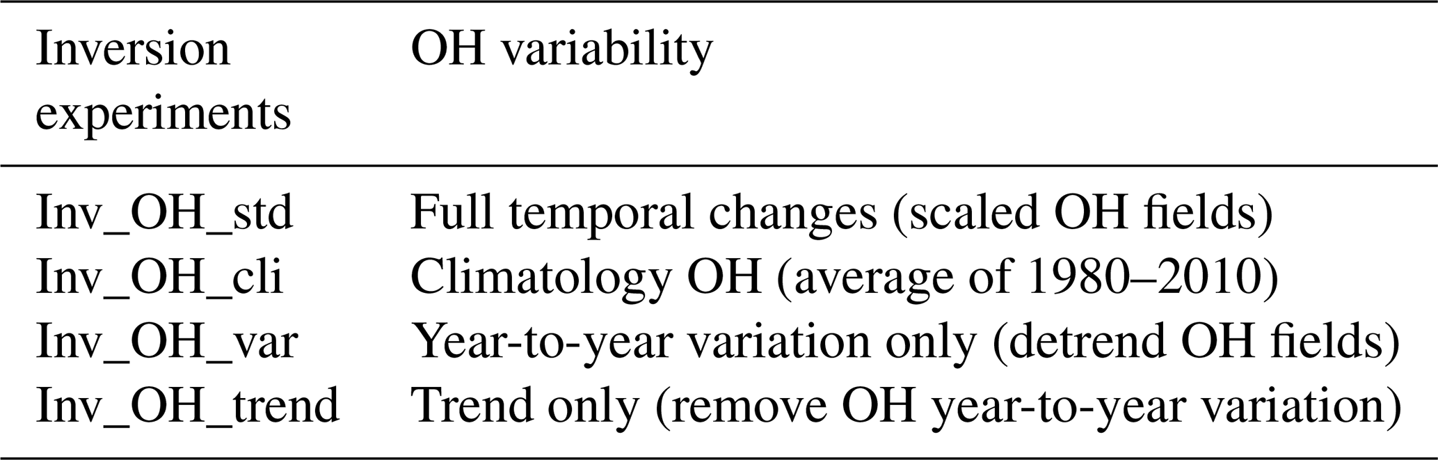
We have designed an ensemble of inversion experiments as listed in Table 1 using the two-box model with each OH field. Here, Inv_OH_std uses the aforementioned scaled OH fields; Inv_OH_cli uses a climatology of each OH field, which is constant over the years and correspond to an average over 1980–2010; Inv_OH_var stands for the inversion using the detrended OH (only keeping the year-to-year variations); Inv_OH_trend uses the OH without the year-to-year variability (retaining only the trend). By comparing Inv_OH_cli with Inv_OH_std, Inv_OH_var, and Inv_OH_trend, it is possible to assess the influence of total OH temporal changes, year-to-year variations, and OH trends, respectively, on the overall CH₄ changes. The box model inversions are conducted from 1984 to 2012 (2010 OH fields are used for 2011 and 2012). The first and last 2 years are treated as spin-up and spin-down, and we only analyze the inversion results over 1986–2010.

Table 1 Two-box model inversion experiments.

We have conducted two 4D variational inversions, Inv_OH_std and Inv_OH_cli, using the multimodel mean OH field to test the influence of OH temporal variations on the top-down estimates of global to regional CH₄ emissions. The LMDz inversions are conducted for four time periods (1994–1997, 1996–1999, 2000–2004, and 2006–2010; Sect. 3.4). We only spin-up and spin-down the 4D variational inversions for 1 year to save computing time. The four time periods are chosen to represent the transition from La Niña (1995–1996) to El Niño (1997–1998) years and the years of stagnated (2001–2003) and renewed growth (2007–2009) of observed CH₄.

3 Results

3.1 Decadal OH trends and year-to-year variability

All CCMI models simulate positive OH trends from 1980 to 2010 after removing the year-to-year variability (Fig. 1a), consistent with previous analyses of CCMI OH fields (Zhao et al., 2019; Nicely et al., 2020) and model results of the Aerosol Chemistry Model Intercomparison Project (Stevenson et al., 2020). The multimodel mean [OH]${}_{{\text{GM-CH}}_{\mathrm{4}}}$ increased by 0.7 ×10⁵ molec cm⁻³ from 1980 to 2010. The growth rates in [OH]${}_{{\text{GM-CH}}_{\mathrm{4}}}$ are estimated as ∼ 0.03 ×10⁵ molec cm⁻³ yr⁻¹ (0.3 % yr⁻¹) during the early 1980s, ∼ 0.01 ×10⁵ molec cm⁻³ yr⁻¹ (0.1 % yr⁻¹) between the mid-1980s and the late 1990s, and 0.03–0.05 ×10⁵ molec cm⁻³ yr⁻¹ (0.3 %–0.5 % yr⁻¹) since the 2000s. This continuous increase in [OH] is different from the results based on the MCF inversions using the two-box model approach (Turner et al., 2017; Rigby et al., 2017), which yield increases in [OH] from the 1990s to the early 2000s and a decrease in OH afterward.

Figure 1 (a) Annual global tropospheric mean OH concentration ([OH]${}_{{\text{GM-CH}}_{\mathrm{4}}}$, CH₄ reaction weighted) with year-to-year variations removed (represents the OH trend) simulated by CCMI models. The black line is the multimodel mean, and associated error bars are standard deviations of different model results (also for panel b). (b) Anomaly of detrended and deseasonalized monthly mean [OH]${}_{{\text{GM-CH}}_{\mathrm{4}}}$ (represents the year-to-year variations in OH). Red bars indicate that the multimodel-simulated [OH]${}_{{\text{GM-CH}}_{\mathrm{4}}}$ has statistically significant (P < 0.05) positive anomalies; blue bars indicate statistically significant negative anomalies; and grey bars indicate statistically nonsignificant anomalies. (c) Bimonthly Multivariate ENSO Index (MEI.v2, 2020).

The ensemble of the anomaly of detrended [OH]${}_{{\text{GM-CH}}_{\mathrm{4}}}$ (Fig. 1b) shows a strong anticorrelation (r = −0.50) with the bimonthly Multivariate ENSO Index Version 2 (MEI.v2, 2020; Fig. 1c and Sect. S3; Zhang et al., 2019), with higher [OH]${}_{{\text{GM-CH}}_{\mathrm{4}}}$ during La Niña and lower [OH]${}_{{\text{GM-CH}}_{\mathrm{4}}}$ during El Niño. From 1980 to 2010, the CCMI model simulations show several negative anomalies of [OH]${}_{{\text{GM-CH}}_{\mathrm{4}}}$, the three largest reaching as high as −0.4 ± 0.2 ×10⁵ molec cm⁻³ (−4 ± 2 %) during 1982–1983 and 1991–1992 and −0.5 ± 0.4 ×10⁵ molec cm⁻³ (−5 ± 4 %) during 1997–1998. The negative [OH]${}_{{\text{GM-CH}}_{\mathrm{4}}}$ anomalies during 1982–1983 and 1997–1998 correspond to the two strongest El Niño events (MEI > 2.5). During 1991–1992, the negative [OH]${}_{{\text{GM-CH}}_{\mathrm{4}}}$ anomaly corresponds to both the weaker El Niño event (MEI up to 2.0), and the eruption of Mount Pinatubo. During other weak El Niño events (1986–1987, 2002–2003, 2004–2005, and 2006–2007), the multimodel mean [OH]${}_{{\text{GM-CH}}_{\mathrm{4}}}$ shows smaller negative anomalies of 1 %–2 %. Only the negative OH anomaly during 2006–2007 (2 ± 1 %) is simulated by all models during the four weak El Niño events. The negative anomalies are consistent with an up to 9 % reduction in [OH] during 1997–1998 simulated by TOMCAT-GLOMAP as shown by Rowlinson et al. (2019), as well as with a 5 % reduction in [OH] over tropical regions during 1991–1993 constrained by MCF observations (Bousquet et al., 2006). During La Niña events, the [OH]${}_{{\text{GM-CH}}_{\mathrm{4}}}$ shows ∼ 2 % positive anomalies, resulting in more than a 6 % increase in OH (max–min) during 1983–1985, 1992–1994, and 1998–2000.

The negative [OH]${}_{{\text{GM-CH}}_{\mathrm{4}}}$ anomalies during strong El Niño events correspond to the highest growth rates of the CH₄ mixing ratio from the surface observations (Dlugokencky, 2020), which are 14 ± 0.6 ppbv yr⁻¹ in 1991 and 12 ± 0.8 ppbv yr⁻¹ in 1998 (Fig. S1). The positive anomalies of [OH]${}_{{\text{GM-CH}}_{\mathrm{4}}}$ during La Niña events correspond to a much smaller CH₄ growth (e.g., 4 ± 0.6 ppbv yr⁻¹ in 1993 and 2 ± 0.8 ppbv yr⁻¹ in 1999) compared with that during the adjacent El Niño years (Fig. S1).

3.2 Factors controlling OH trends and year-to-year variability

The changes in tropospheric [OH] are due to changes in the balance of production and loss. Here we assess the drivers of OH year-to-year variations and trend by calculating the OH production and loss processes listed in Table 2 following Murray et al. (2013, 2014) and Lelieveld et al. (2016). The multimodel calculated OH production and loss in the troposphere averaged over 1980–2010 is 209 ± 12 Tmol yr⁻¹, similar to the ∼ 200 Tmol yr⁻¹ reported by Murray et al. (2014). Of the total OH production, 46 % (96 ± 2 Tmol yr⁻¹) is from primary production (O(¹D) + H₂O). Two main secondary productions of NO + HO₂ and O₃+ HO₂ account for 30 % (63 ± 4 Tmol yr⁻¹) and 13 % (26 ± 2 Tmol yr⁻¹), respectively. For the OH loss, reactions with CO and CH₄ account for 39 % (82 ± 4 Tmol yr⁻¹) and 15 % (32 ± 1 Tmol yr⁻¹), respectively. We have also calculated the OH loss by reactions with isoprene (C₅H₈) and formaldehyde (CH₂O), which both remove 6 % of OH, reflecting the influences of NMVOCs from natural and anthropogenic sources, respectively. Besides, there are 12 % of OH production and 33 % of OH loss not analyzed here due to lack of data in the CCMI model outputs (e.g., output of OH loss due to reaction with NMVOCs included in different models).

Table 2 Multimodel mean ± standard deviation (SD) of annual total OH production (P) and loss (L) in teramoles per year and percentage contribution of each production and loss process to total OH production and loss estimated with multimodel mean OH fields^∗.

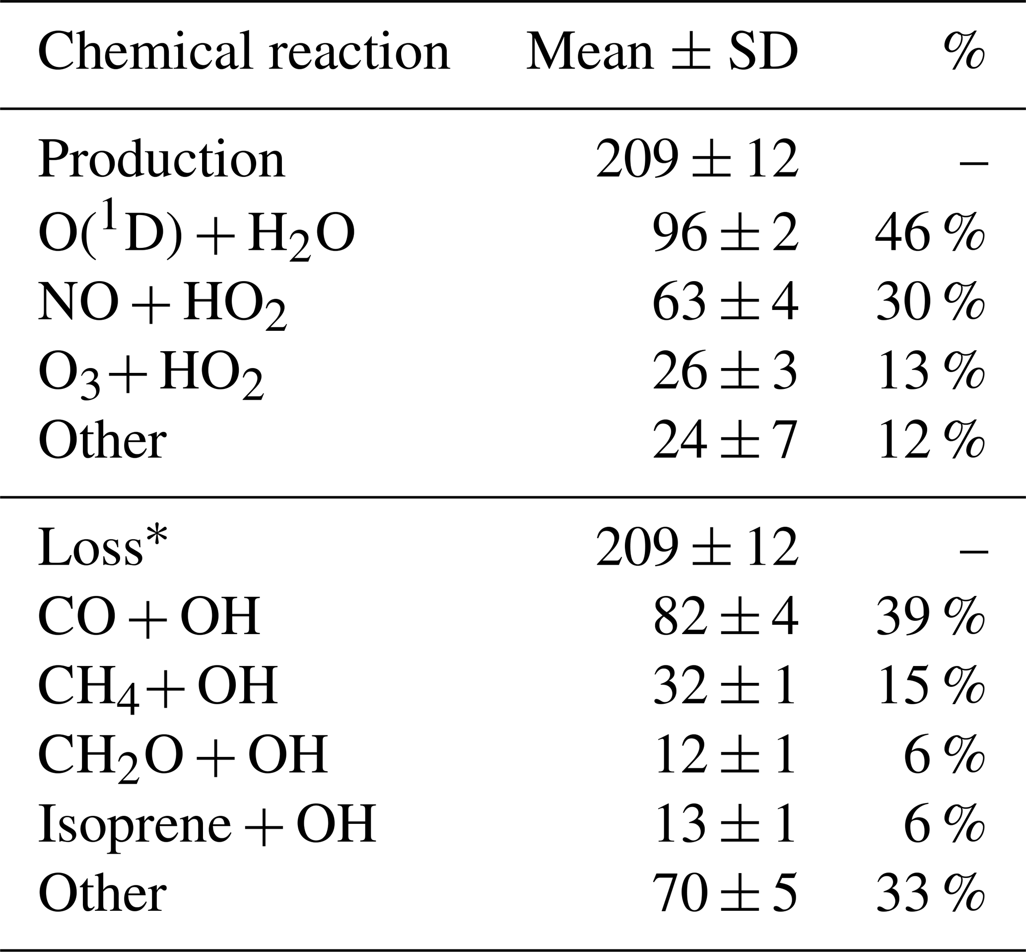
^∗ The OH production and loss of the EMAC model are not included in the table since total OH production and loss are not given by the EMAC model.

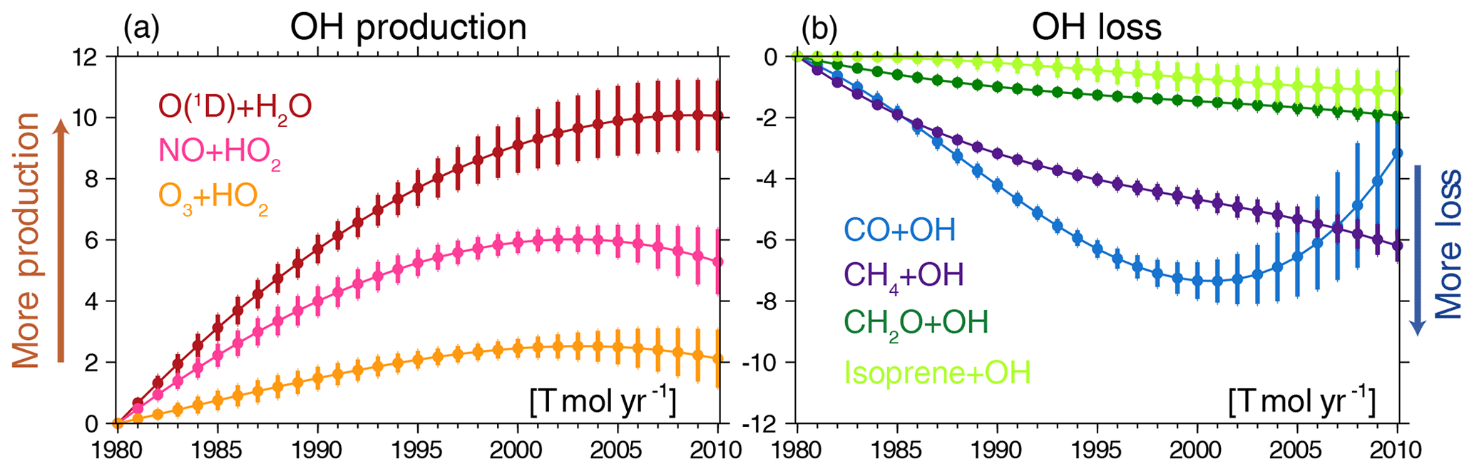
Figure 2 Annual total OH tendency (Tmol yr⁻¹) from chemical reactions with respect to the year 1980 with year-to-year variations removed. The positive and negative tendencies represent OH production (a) and loss processes (b), respectively.

Figure 2 shows the changes in the trends of OH production and loss processes (year-to-year variations are removed) with respect to the year 1980. The OH primary production (O(¹D) + H₂O) shows a large increase of 10 ± 1 Tmol yr⁻¹ from 1980 to 2010, as the dominant driver of the positive OH trend. The increase in OH primary production is due to an increase in both tropospheric O₃ burden (producing O(¹D)) and water vapor (Dentener et al., 2003; Zhao et al., 2019; Nicely et al., 2020). The OH loss from CO increased by 7 ± 0.7 Tmol yr⁻¹ from 1980 to 2001 but then decreased by 4 ± 2 Tmol yr⁻¹ from 2001 to 2010. The negative trend of CO simulated by CCMI models during 2000–2010 is consistent with MOPITT observations over most of the regions (Strode et al., 2016). We find that the decrease in OH loss by CO can explain the accelerated OH increase after 2000, despite a stagnated OH primary production and a slight decrease in the OH secondary production. The OH loss by CH₄, which shows a continuous increase of 6 ± 0.5 Tmol yr⁻¹ from 1980 to 2010, buffers the increase in OH production by NO (5 ± 1 Tmol yr⁻¹). The OH production by O₃+ HO₂ and OH loss by CH₂O and isoprene show smaller changes of 2 ± 1, 2 ± 0.3, and 1 ± 0.6 Tmol yr⁻¹, respectively, during 1980–2010. By comparing the magnitude of the production and loss processes, we conclude that an enhanced OH primary production and changes in OH loss by CO are the most important factors leading to the increased OH trend inferred from CCMI models from 1980 to 2010.

Figures 3 and S2 show the year-to-year variations in the global total OH production and loss due to several processes (calculated after trends have been removed). Year-to-year variations in global [OH] are mainly determined by the primary (O(¹D) + H₂O) and secondary (NO + HO₂; O₃+ HO₂) production and by OH loss due to CO (Fig. 3). Other OH loss processes, including reactions with CH₄, CH₂O, and isoprene, show much smaller year-to-year variations but larger uncertainties (Fig. S2), revealing a larger model spread for these processes.

Figure 3 Anomaly of the detrended annual global total OH tendency from reactions O(¹D) + H₂O, NO + HO₂, O₃+ HO₂, and CO + OH. Black lines are multimodel means, and the error bars are the standard deviations of all CCMI model results. The red, blue, and grey dots and error bars show statistically significant (P < 0.05) positive anomalies, negative anomalies, and statistically nonsignificant anomalies, respectively. Shaded areas represent the El Niño years with more than 5 months of MEI > 1.0.

As shown in Fig. 3, negative anomalies of [OH] during El Niño events are dominated by increased OH loss through the reaction with CO in response to enhanced biomass burning (Fig. S3), which is similar to the conclusions of Rowlinson et al. (2019) and Nicely et al. (2020). During the strong El Niño events in 1982–1983, 1991–1992, and 1997–1998, the OH loss by CO increased by up to 3 ± 0.4, 5 ± 0.6, and 8 ± 0.5 Tmol yr⁻¹, respectively, compared to the mean value of 1980–2010. The increase in OH loss by CO can be partly offset by an increase in OH production. Indeed, in 1998, the OH primary production (O(¹D) + H₂O), OH produced by NO + RO₂, and O₃+ RO₂ increased by 3 ± 0.7, 3 ± 0.5, and 2 ± 0.3 Tmol yr⁻¹, respectively, offsetting most of the OH loss increase. The increase in OH primary production is mainly due to an increase in tropospheric water vapor and O₃ burden during El Niño events (Figs. S3 and S12 in Nicely et al., 2020), while the increase in OH secondary production is caused by enhanced NO_x emissions (Fig. S3) and O₃ formation (Nicely et al., 2020) related to biomass burning as well as to more HO₂ formation by CO + OH. As a result, the OH year-to-year variations found here are much smaller than those estimated by Nguyen et al. (2020), who mainly considered the response of OH to enhanced CO emissions during the El Niño events. The positive anomaly in OH primary production (0.2 ± 0.5 Tmol yr⁻¹) is not significant during the 1991–1992 El Niño event, maybe due to the absorption of ultraviolet (UV) radiation by volcanic SO₂ and scattering of UV radiation by sulfate aerosols as well as to the reduction in tropospheric water vapor after the eruption of Mount Pinatubo (Bândă et al., 2016; Soden et al., 2002). Thus, the negative [OH] anomaly during the weak El Niño event in 1991–1992 is potentially being enhanced by the eruption of Mount Pinatubo. Previous studies have shown that NO_x emissions from lightning can contribute to the OH interannual variability (Murray et al., 2013; Turner et al., 2018). In addition, soil NO_x emissions depend on temperature and soil humidity (Yienger and Levy, 1995), which vary during the El Niño events. The year-to-year variations in NO_x emissions from lightning show large differences among CCMI models (Fig. S4), and only EMAC and GEOSCCM apply interactive soil NO_x emissions that vary with meteorology conditions (Morgenstern et al., 2017) based on Yienger and Levy (1995). Thus NO_x emissions from lightning and soil mainly contribute to intermodel differences instead of showing a consistent response to El Niño.

Using a machine learning method, Nicely et al. (2020) attributed the positive [OH] trend simulated by the CCMI models mainly to the increase in tropospheric O₃, J(O¹D), NO_x, and H₂O, and attributed [OH] interannual variations to CO changes. Overall, the explanations of the drivers of OH year-to-year variations and trends found in our process analysis are broadly consistent with those reported by Nicely et al. (2020), and we emphasize that the decrease in CO emissions and concentrations after 2000 (Zheng et al., 2019) is important for determining the accelerated positive OH trend.

3.3 Impact of OH variation on the top-down estimation of CH₄ budget

Figure 4a shows the anomaly of global total CH₄ emissions estimated by inv_OH_std (nine scaled OH fields; orange line) and inv_OH_cli (nine climatological OH; blue line) using the two-box model during 1986–2010. With the climatological OH fields (blue line), the top-down-estimated CH₄ emissions show no clear trend before 2005, with large positive anomalies during strong El Niño years. There are two peaks of positive CH₄ emission anomalies during this period: 10 Tg yr⁻¹ in 1991 and 14 Tg yr⁻¹ in 1998. From 2005 to 2008, the CH₄ emissions show a large increase of 26 Tg yr⁻¹. The CH₄ emissions averaged over 2006–2010 are 20 Tg yr⁻¹ higher than over 2000–2005, consistent with the 17–22 Tg yr⁻¹ estimated by an ensemble of inversions in Kirschke et al. (2013).

Figure 4 (a) Anomaly of global total CH₄ emissions using scaled CCMI OH fields (orange line, Inv_OH_std), and climatological OH (blue, Inv_OH_cli) estimated by a two-box model inversion. The anomalies are calculated by comparison with the climatological mean CH₄ emissions of Inv_OH_cli over 1986–2010. (b–d) Influences of (b) total OH temporal variations (OH year-to-year variation and trend, Inv_OH_std minus Inv_OH_cli), (c) OH year-to-year variations (Inv_OH_var minus Inv_OH_cli), and (d) OH trend (Inv_OH_trend minus Inv_OH_cli) on box-model-estimated global total CH₄ emissions. The black lines are the mean of inversion results with different OH fields, and the boxes are ±1 standard deviation. The boxes with filled blue and red show OH leads to statistically significant (P < 0.05) differences between the two inversions.

The OH temporal variations are found to largely influence the interannual changes in top-down-estimated CH₄ emissions (orange line of Fig. 4a), with differences between the two inversions reaching up to more than 15 Tg yr⁻¹ (Fig. 4b). The contributions from the OH year-to-year variations and trends are also shown in Fig. 4. The negative anomalies of OH during El Niño years reduce the unusually high top-down-estimated CH₄ emissions in 1991–1992 by 7 ± 3 Tg yr⁻¹ and in 1998 by 10 ± 3 Tg yr⁻¹ (Fig. 4c). As a result, the high-emission peaks to match the observed CH₄ mixing-ratio growth in 1991 (14 ppb yr⁻¹) and 1998 (12 ppbv yr⁻¹), as estimated using the climatological OH, are largely reduced.

The identified positive OH trend leads to an additional 23 ± 9 Tg yr⁻¹ increase in CH₄ emissions from 1986 to 2010 (Fig. 4d). During 1986–2005, the mean CH₄ emissions, as estimated with the scaled OH, show a positive trend of 0.6 ± 0.4 Tg yr⁻² (P < 0.05). Increased CH₄ emissions offset the increase in the OH sink to match the observations. From 2005 to 2008, in contrast to previous studies, which attribute the increased observed CH₄ mixing ratios to decreased OH based on MCF inversions (Turner et al., 2017; Rigby et al., 2017), the increasing OH trend simulated by CCMI models results in an additional 5 ± 2 Tg yr⁻¹ CH₄ emission increase in the inversion to match the observations.

We compare the inversion using the two-box model (“×” in Fig. 5) with the results from the variational approach (bars in Fig. 5), using the multimodel mean OH field, to evaluate the performance of the simplified two-box model inversions. Despite the limitations inherent to two-box model inversions, such as treatment of interhemispheric transport, stratospheric loss, and the impact of spatial variability (Naus et al., 2019), the two-box model inversion estimates similar temporal changes in CH₄ emissions and losses compared to the variational approach for the four periods, as well as to their response to OH changes (Fig. 5), on a global scale. Such comparisons reinforce the reliability of the conclusions made from the two-box model inversions regarding changes in the global total CH₄ budget.

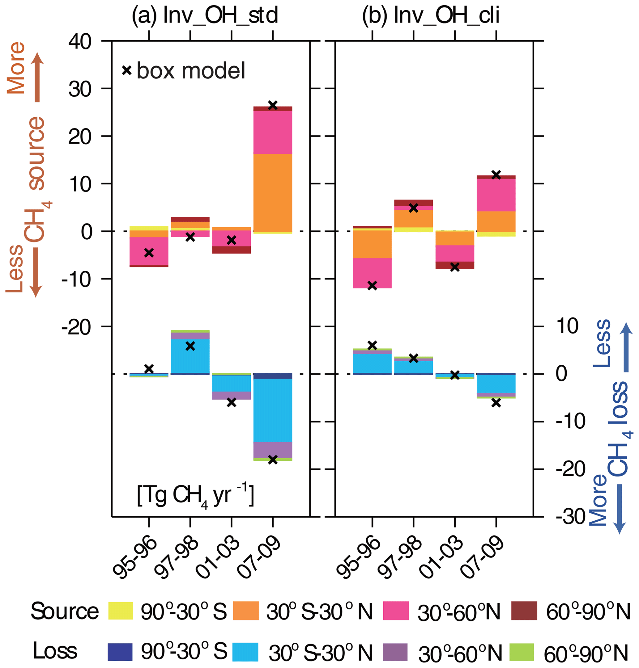
Figure 5 Anomaly of CH₄ emissions and losses estimated by variational 4D inversions (bars) and by two-box model inversions (“×”) using a multimodel mean scaled OH (Inv_OH_std, a) and climatological OH (b) during four time periods. The anomalies are calculated by comparison with the mean CH₄ emissions of Inv_OH_cli over the four time periods (494 Tg). The total emissions and loss over southern extratropical regions (90–30^∘ S), the tropics (30^∘ S–30^∘ N), the northern temperate regions (30–60^∘ N), and the northern boreal regions (60–90^∘ N) are shown by different colors within each bar.

The variational inversions allow us to assess the regional contribution of the drivers to observed atmospheric CH₄ mixing-ratio changes. Here, as a synthesis, we focus on four latitude bands (Fig. 5 and Table S2), including the southern extratropical regions (90–30^∘ S), the tropical regions (30^∘ S–30^∘ N), and the northern temperate (30–60^∘ N) and boreal (60–90^∘ N) regions. On average, OH over the tropical and northern temperate regions removes 74 % and 14 % of global total atmospheric CH₄, respectively.

Between the periods 1995–1996 and 1997–1998, if one does not consider the OH temporal variations (Inv_OH_cli), the CH₄ loss by OH shows a slight increase of 2 Tg yr⁻¹ due to an increase in atmospheric CH₄ mixing ratios. The main driver of observed atmospheric CH₄ mixing-ratio changes is the 10 Tg yr⁻¹ increase in CH₄ emissions over the tropics and the 7 Tg yr⁻¹ increase over the northern temperate regions (Fig. 5b and Table S2). When the multimodel mean OH temporal variations are included (Inv_OH_std), the negative anomaly of OH in 1997–1998 leads to a 9 Tg yr⁻¹ decrease in CH₄ loss in 1997–1998 compared to 1995–1996, of which 7 Tg yr⁻¹ (78 %) is contributed by the tropical regions (Fig. 5a). As a result, the decrease in CH₄ loss by OH contributes a bit more to match the observed CH₄ mixing-ratio increase during the El Niño periods than the changes in CH₄ emissions (a global increase of 8 Tg yr⁻¹). The emission increases from 1995–1996 to 1997–1998 over the tropics, and the northern temperate regions are reduced to 3 and 5 Tg yr⁻¹ (Fig. 5a, Inv_OH_std), respectively, which is similar to the inversion results given by Bousquet et al. (2006).

From the period 2001–2003 to 2007–2009, positive OH trends lead to a 13 Tg yr⁻¹ increase in the CH₄ loss, of which 10 Tg yr⁻¹ (76 %) originates from the tropics (Inv_OH_std, Fig. 5a). In response to increased CH₄ losses, the increase in optimized emissions over tropical regions (16 Tg yr⁻¹, Inv_OH_std) is more than twice that of the inversion using climatological OH (7 Tg yr⁻¹, Inv_OH_ cli). The emission increases during the two periods over the northern region show a smaller change of 2 Tg yr⁻¹ (12 Tg yr⁻¹ estimated by Inv_OH_std versus 10 Tg yr⁻¹ by Inv_OH_cli, Fig. 5). The variational inversions show that the OH temporal variations are most critical for top-down estimates of CH₄ budgets over the tropical regions since OH over tropical regions shows larger interannual variations and trends than middle- to high-latitude regions (Fig. S5) and most of the CH₄ (74 %) is removed from the atmosphere by OH over the tropical regions.

4 Conclusion and discussion

Based on the simulations from the CCMI, we explore the response of OH fields to changes in climate and anthropogenic and natural emissions and their impact on the top-down estimates of CH₄ emissions during 1980–2010 based on a model perspective. We find that although CCMI models simulated rather different global total burdens of OH (Zhao et al., 2019), they show very similar patterns in temporal variations, including (1) negative anomalies during El Niño years, which are mainly driven by an elevated OH loss by reaction with CO from enhanced biomass burning, despite a partial buffering through enhanced OH production, and (2) a continuous increase in OH from 1980, which is mostly contributed by OH primary production, and acceleration after 2000 due to reduced CO emissions. By conducting inversions using a two-box model and a variational approach together with the ensemble of CCMI OH fields, we find that (1) the OH year-to-year variations can largely reduce the CH₄ emission increase (by up to 10 Tg yr⁻¹) needed to match the observed CH₄ increase during El Niño years and (2) the positive OH trend results in a 23 ± 9 Tg yr⁻¹ additional increase in optimized emissions from 1986 to 2010 compared to the inversions using constant OH. The variational inversions also show that OH temporal variations mainly influence top-down estimates of CH₄ emissions over tropical regions.

The responses of OH to changes in biomass burning, ozone, water vapor, and lightning NO_x emissions during El Niño years have been recognized by previous studies (Holmes et al., 2013; Murray et al., 2014; Turner et al., 2018; Rowlinson et al., 2019; Nguyen et al., 2020). Here, the consistent temporal variations in CCMI OH fields increase our confidence in the model-simulated response of OH to ENSO as a result of several nonlinear chemical processes. We estimated that the negative OH anomaly in 1998 reduces the high top-down-estimated CH₄ emissions by 10 ± 3 Tg yr⁻¹, ∼ 40 % smaller than the reduction estimated by Butler et al. (2005; 16 Tg yr⁻¹), which only includes the OH reduction response to enhanced biomass burning CO emissions. The smaller CH₄ emission reduction (OH anomaly) estimated with CCMI OH fields may reflect the significance of considering multiple chemical processes as included in the 3D atmospheric chemistry model in capturing OH variations and inverting for CH₄ emissions. One of the largest uncertainties is NO_x emissions from lightning, which have been proven to contribute to year-to-year variations in OH (Murray et al., 2013; Turner et al., 2018) but here show a large spread among CCMI models. In addition, NO_x emissions from soil may also change during El Niño years. Improving estimates of NO_x emissions from lightning based on satellite observations (Murray et al., 2013) and a better representation of the interactive NO_x emissions from the soil are critical for improving the model simulation of OH temporal variability and for top-down estimates of year-to-year variations in CH₄ emissions.

The positive trend of OH after the mid-2000s, which results in enhanced top-down-estimated CH₄ emissions over the tropics, is opposite to those constrained by MCF inversions (Turner et al., 2017; Rigby et al., 2017). The processes that control the model-simulated positive OH trend discussed in this study are supported by current studies based on observations, including decreased CO emissions (Zheng et al., 2019), small variations in global NO_x emissions (Miyazaki et al., 2017), and an increase in tropospheric ozone (Ziemke et al., 2019) and water vapor (Chung et al., 2014). However, the CCMI models still show biases that are related to OH production and loss. For example, these include an underestimation of CO especially over the Northern Hemisphere compared with the surface and satellite observations (Naik et al., 2013; Strode et al., 2016) and bias in the atmospheric total O₃ column (Zhao et al., 2019). In addition, changes in aerosols (Tang et al., 2003) and atmospheric circulation such as the Hadley cell expansion (Nicely et al., 2018) are not discussed in this study. Given the uncertainties in both the atmospheric chemistry model simulated (Naik et al., 2013; Zhao et al., 2019) and MCF-constrained OH (Bousquet et al., 2005; Prather and Holmes, 2017; Naus et al., 2019) and the large discrepancy between the two methods, the OH trend after the mid-2000s remains an open problem, and more effort is required in developing both methods to close the gap.

The temporal variations in OH, which are generally not well constrained in current top-down estimates of CH₄ emissions, imply potential additional uncertainties in the global CH₄ budget (Saunois et al., 2017; Zhao et al., 2020). The tropical regions, where top-down-estimated CH₄ emissions show the largest sensitivity to OH changes, represent more than 60 % of CH₄ emissions worldwide (Saunois et al., 2016). The tropical CH₄ emissions are dominated by wetland emissions, in which large uncertainties exist in both bottom-up and top-down studies (Saunois et al., 2016, 2017). The variational inversions using OH with temporal variations attribute the observed rising CH₄ growth during El Niño to the reduction in CH₄ loss instead of to enhanced emissions over the tropics, which is consistent with process-based wetland models that estimated wetland CH₄ emission reductions at the beginning of the El Niño event (Hodson et al., 2011; Zhang et al., 2018). Also, the negative OH anomaly can reduce the top-down-estimated biomass burning CH₄ emission spikes during El Niño events, consistent with the conclusions given by Bousquet et al. (2006). Future climate projections show that the extreme El Niño events will be more frequent under a warmer climate (Berner et al., 2020), which may enhance the fluctuations in [OH]. Furthermore, the changes in anthropogenic emissions, such as expected decreases in NO_x emissions (Lamarque et al., 2013), can also affect the OH trends. Our research emphasizes the importance of considering climate changes and chemical feedbacks related to OH in future CH₄ budget research.