the Creative Commons Attribution 4.0 License.
the Creative Commons Attribution 4.0 License.
 | 13 Aug 2020
Influences of hydroxyl radicals (OH) on top-down estimates of the global and regional methane budgets
Yuanhong Zhao
Marielle Saunois
Philippe Bousquet
Antoine Berchet
Michaela I. Hegglin
Josep G. Canadell
Robert B. Jackson
Edward J. Dlugokencky
Ray L. Langenfelds
Michel Ramonet
Doug Worthy
The hydroxyl radical (OH), which is the dominant sink of methane (CH4), plays a key role in closing the global methane budget. Current top-down estimates of the global and regional CH4 budget using 3D models usually apply prescribed OH fields and attribute model–observation mismatches almost exclusively to CH4 emissions, leaving the uncertainties due to prescribed OH fields less quantified. Here, using a variational Bayesian inversion framework and the 3D chemical transport model LMDz, combined with 10 different OH fields derived from chemistry–climate models (Chemistry–Climate Model Initiative, or CCMI, experiment), we evaluate the influence of OH burden, spatial distribution, and temporal variations on the global and regional CH4 budget. The global tropospheric mean CH4-reaction-weighted [OH] ([OH]) ranges 10.3–16.3×10⁵ molec cm−3 across 10 OH fields during the early 2000s, resulting in inversion-based global CH4 emissions between 518 and 757 Tg yr−1. The uncertainties in CH4 inversions induced by the different OH fields are similar to the CH4 emission range estimated by previous bottom-up syntheses and larger than the range reported by the top-down studies. The uncertainties in emissions induced by OH are largest over South America, corresponding to large inter-model differences of [OH] in this region. From the early to the late 2000s, the optimized CH4 emissions increased by 22±6 Tg yr−1 (17–30 Tg yr−1), of which ∼25 % (on average) offsets the 0.7 % (on average) increase in OH burden. If the CCMI models represent the OH trend properly over the 2000s, our results show that a higher increasing trend of CH4 emissions is needed to match the CH4 observations compared to the CH4 emission trend derived using constant OH. This study strengthens the importance of reaching a better representation of OH burden and of OH spatial and temporal distributions to reduce the uncertainties in the global and regional CH4 budgets.
- Article
(3968 KB) - Full-text XML
- Companion paper 1
- Companion paper 3
-
Supplement
(1698 KB) - BibTeX
- EndNote


Methane (CH4) plays an important role in both climate change and air quality as a major greenhouse gas and tropospheric ozone precursor (Ciais et al., 2013). CH4 is emitted from various anthropogenic sources including agriculture, waste, fossil fuel, and biomass burning, as well as natural sources including wetlands and other freshwater systems, geological sources, termites, and wild animals. CH4 is removed from the atmosphere mainly by reaction with the hydroxyl radical (OH) (Saunois et al., 2016, 2017). Tropospheric CH4 levels have more than doubled between the 1850s and the present day (Etheridge et al., 1998) in response to anthropogenic emissions and climate variabilities, leading to about 0.62 W m−2 of radiative forcing (Etminan et al., 2016) and increases in tropospheric ozone levels of ∼5 ppbv (Fiore et al., 2008). The global CH4 atmospheric mixing ratio stabilized in the early 2000s but resumed growing at a rate of ∼5 ppbv yr−1 or more starting in 2007 (Dlugokencky, NOAA/ESRL, 2019).
Explaining the CH4 stabilization and renewed growth requires an accurate estimation of the CH4 budget and its evolution, as the source–sink imbalance that is responsible for the contemporary CH4 yearly growth only accounts for 3 % of the total CH4 burden (Turner et al., 2019). To reconcile the uncertainties in the current estimation of CH4 emissions from various sources, the Global Carbon Project integrates top-down and bottom-up approaches (Kirschke et al., 2013; Saunois et al., 2016, 2017, 2020). However, gaps remain in global and regional CH4 emissions estimated by top-down and bottom-up approaches, as well as within each approach (Kirschke et al., 2013; Saunois et al., 2016; Bloom et al., 2017). The top-down method, which optimizes emissions by assimilating observations in an atmospheric inversion system, is expected to reduce uncertainties of bottom-up estimates. Among the remaining causes of uncertainties in the global methane budget, the representation of CH4 sinks, mainly from OH oxidation, is one of the largest, as seen by process-based models for atmospheric chemistry (Saunois et al., 2017).
OH is the most important tropospheric oxidizing agent determining the lifetime of many pollutants and greenhouse gases including CH4 (Levy, 1971). A small perturbation of OH can result in significant changes in the budget of atmospheric CH4 (Turner et al., 2019). At the global scale, tropospheric OH is mainly produced by the reaction of excited oxygen atoms (O(1D)) with water vapor (primary production) but also by the reaction of nitrogen oxide (NO) and ozone (O3) with hydroperoxyl radicals (HO2) and organic peroxy radicals (RO2) (secondary production). At regional scales, photolysis of hydrogen peroxide and oxidized volatile organic compound (VOC) photolysis can be important depending on the chemical environment (Lelieveld et al., 2016). OH is rapidly removed by carbon monoxide (CO), methane (CH4), and non-methane volatile organic compounds (NMVOCs) (Logan et al., 1981; Lelieveld et al., 2004). Tropospheric OH has a very short lifetime of a few seconds (Logan et al., 1981; Lelieveld et al., 2004), hindering estimates of global OH concentrations ([OH]) through direct measurements and limiting our ability to estimate the global CH4 sink.
Global tropospheric [OH] is approximately 1×10⁶ molec cm−3 as calculated by atmospheric chemistry models (Naik et al., 2013; Voulgarakis et al., 2013, Zhao et al., 2019) and inversions of 1,1,1-trichloroethane (methyl chloroform, MCF) (Prinn et al., 2001; Bousquet et al., 2005; Montzka et al., 2011; Cressot et al., 2014), resulting in a chemical lifetime of ∼9 years for tropospheric CH4 (Prather et al., 2012; Naik et al., 2013). However, accurate estimations of [OH] magnitude, distributions, and year-to-year variations needed for CH4 emission optimizations are still pending (Prather et al., 2017; Turner et al., 2019). For global tropospheric [OH], both MCF inversions and atmospheric chemistry model intercomparisons give a 10%–15 % uncertainty (Prinn et al., 2001; Bousquet et al., 2005; Naik et al., 2013; Zhao et al., 2019). For [OH] spatial distributions, MCF-based inversions generally infer similar mean [OH] over both hemispheres (Bousquet et al., 2005; Patra et al., 2014), while atmospheric chemistry models generally give [OH] Northern Hemisphere to Southern Hemisphere (N∕S) ratios above 1 (e.g., Naik et al., 2013; Zhao et al., 2019). For [OH] year-to-year variations, some studies have estimated magnitudes significant enough to help explain part of the stagnation in atmospheric CH4 concentrations during the early 2000s (Rigby et al., 2008, 2017; McNorton et al., 2016; Dalsøren et al., 2016; Turner et al., 2017), whereas others show smaller trends and interannual variations of [OH] (Montzka et al., 2011; Naik et al., 2013; Voulgarakis et al., 2013; Zhao et al., 2019). In a recent study, Zhao et al. (2019) simulated atmospheric CH4 with an ensemble of OH fields and showed that uncertainties in [OH] variations could explain up to 54 % of model–observation discrepancies in surface CH4 mixing ratio changes from 2000 to 2016.
Current top-down estimates of the global CH4 budget usually apply prescribed and constant [OH] simulated by atmospheric chemistry models and attribute model–observation mismatches exclusively to CH4 emissions (Saunois et al., 2017). However, the OH fields simulated by atmospheric chemistry models show some uncertainties in both global burden and spatial–temporal variations (Naik et al., 2013; Zhao et al., 2019). The role of OH variations in the top-down estimates of CH4 emissions has been evaluated using two box model inversions with surface observations (e.g., Rigby et al., 2017; Turner et al., 2017; Naus et al., 2019) and 3D models that optimize CH4 emissions together with [OH] by assimilating surface observations (Bousquet et al., 2006) or satellite data (Cressot et al., 2014; McNorton et al., 2018; Zhang et al., 2018; Maasakkers et al., 2019). The proxy-based constraints usually optimize [OH] on a global or latitudinal scale, with the impact of OH vertical and horizontal distributions being less quantified to date. Also, proxy methods do not allow access to underlying processes as direct chemistry modeling does (Zhao et al., 2019). This paper follows the work of Zhao et al. (2019), wherein we analyzed in detail 10 OH fields derived from atmospheric chemistry models considering different chemistry, emissions, and dynamics (Patra et al., 2011; Szopa et al., 2013; Hegglin and Lamarque, 2015; Morgenstern et al., 2017; Zhao et al., 2019; Terrenoire et al., 2020). We now aim to build on this previous paper to estimate the impact of these OH fields on methane emissions as inferred by an atmospheric 4D variational inversion system. To do so, we use each of the OH fields in the 4D variational inversion system PYVAR-LMDz based on the LMDZ-SACS (Laboratoire de Météorologie Dynamique model with the Zooming-capability Simplified Atmospheric Chemistry System) 3D chemical transport model to evaluate the influence of OH distributions and variations on the top-down estimated global and regional CH4 budget. Section 2 briefly describes the OH fields and their characteristics and underlying processes (see also Zhao et al., 2019, for more details), the inversion method, and the setups of inversion experiments. Section 3 illustrates the influence of OH on the top-down estimation of CH4 budgets and variations, specifically the following: (i) global, regional, and sectoral CH4 emissions (Sect. 3.1); (ii) emission changes between the early 2000s and late 2000s (Sect. 3.2); and (iii) year-to-year variations in methane emissions (Sect. 3.3). Section 4 summarizes the results and discusses the impact of OH on the current CH4 budget.
Table 1Global tropospheric mean [OH] (×105 molec cm−3) and interhemispheric OH ratios (N∕S) averaged over 2000–2002 for 10 OH fields used in this study. The global tropospheric [OH] weighted by reaction with CH4 ([OH]) and weighted by dry air mass ([OH]GM−M) are both given.

∗ The OH fields simulated by SOCOL3 and MOCAGE are excluded.
2.1 OH fields
In this study, we test the 10 OH fields presented in by Zhao et al. (2019), including 7 OH fields simulated by chemistry–transport and chemistry–climate models from Phase 1 of the Chemistry–Climate Model Initiative (CCMI) (Hegglin and Lamarque, 2015; Morgenstern et al., 2017), 2 OH fields simulated by the Interaction with Chemistry and Aerosols (INCA) model coupled to the general circulation model of the Laboratoire de Météorologie Dynamique (LMD) model (Hauglustaine et al., 2004; Szopa et al., 2013), and 1 OH field from the TransCom-CH4 intercomparison exercise (Patra et al., 2011) (Table 1).
The CCMI conducted simulations with 20 state-of-the-art atmospheric chemistry–climate and chemistry–transport models to evaluate model projections of atmospheric composition (Hegglin and Lamarque, 2015; Morgenstern et al., 2017). To force atmospheric inversions during 2000–2010, we use OH fields from 7 of the 20 CCMI model simulations of REF-C1 experiments (Table 1), which were driven by observed sea surface temperatures and state-of-the-art historical forcings (covering 1960–2010). For the inversions after 2010 (only with the CESM1-WACCM model; see Sect. 2.3), we apply interannual variations of OH generated from REF-C2 experiments, which were driven by sea surface conditions calculated by the online-coupled ocean and sea ice modules. Although all of the CCMI models use the same anthropogenic emission inventories, the simulated OH fields show different spatial and vertical distributions. The inter-model differences of OH burden and vertical distributions are mainly attributed to differences in chemical mechanisms related to NO production and loss. The differences in [OH] spatial distributions are due to applying different natural emissions: for example, primary biogenic VOC emissions and NO emissions from soil and lightning (Zhao et al., 2019). As a result, the regions dominated by natural emissions (e.g., South America, central Africa) show the largest inter-model differences in [OH] (Fig. S1 in the Supplement). The CCMI models consistently simulated a positive OH trend during 2000–2010, mainly due to more OH production by NO than loss by CO over East and Southeast Asia and a positive trend of water vapor over the tropical regions (Zhao et al., 2019; Nicely et al., 2020). More details can be found in Zhao et al. (2019) and the literature cited herein.
The two INCA OH fields, INCA NMHC-AER-S and INCA NMHC, are simulated by two different versions of the INCA (Interaction with Chemistry and Aerosols) chemical model coupled to LMDz (Szopa et al., 2013; Terrenoire et al., 2020). The main difference between the two simulations is that INCA NMHC-AER-S includes both gas-phase and aerosol chemistry in the whole atmosphere, while INCA NMHC only includes gas-phase chemistry in the troposphere (Szopa et al., 2013; Terrenoire et al., 2020). We also include the climatological OH field used in the TransCom simulations (Patra et al., 2011), which uses the semi-empirical, observation-based OH field computed by Spivakovsky et al. (2000) in the troposphere.
Table 1 summarizes the global tropospheric mean CH4-reaction-weighted [OH] ([OH], [OH] weighted by the reaction rate of OH with CH4 (K)× dry air mass; Lawrence et al., 2001) and dry air-mass-weighted [OH] ([OH]GM−M), as well as interhemispheric ratios (N∕S ratios) calculated with [OH] for the 10 OH fields used in this study. The tropopause height is assumed at 200 hPa following Naik et al. (2013), and the 3D temperature field used to compute [OH] is from ERA-Interim reanalysis meteorology data (Dee et al., 2011). The volume-weighted [OH] was given by Zhao et al. (2019). The [OH] is a better indicator of the global atmospheric oxidizing efficiency for CH4 than [OH]GM−M since the latter is insensitive to the CH4+OH reaction rate increased with temperature (Lawrence et al., 2001). Both the mean value ( molec cm−3) and absolute range (10.3–16.3×10⁵ molec cm−3) of [OH] calculated for the 10 OH fields are larger than those of [OH]GM−M ( molec cm−3 and 9.4–14.4×10⁵ molec cm−3, respectively). This is mainly because the MOCAGE and SOCOL3 OH fields show much higher [OH] near the surface than in the upper troposphere (Zhao et al., 2019). The interhemispheric OH ratios range from 1.0 to 1.5, which is larger than ones derived from MCF inversions (e.g., Bousquet et al., 2005; Patra et al., 2014), partly explained by the underestimation of CO in the Northern Hemisphere by atmospheric chemistry models (Naik et al., 2013). A comprehensive analysis of the spatial and vertical distributions of these OH fields was presented in Zhao et al. (2019).
2.2 Inverse method
We conduct an ensemble of variational inversions of the CH4 budget that rely on Bayes' theorem (Chevallier et al., 2005) with the same set of atmospheric observations of CH4 mixing ratios but different prescribed monthly mean OH fields as described in Sect. 2.1. A variational data assimilation system optimizes CH4 emissions and sinks by minimizing the cost function J, defined as
where x is the control vector that includes total CH4 emissions per 10 d at the model resolution of 3.75∘ longitude latitude and initial conditions at longitudinal and latitudinal bands of ; xb is the prior of the control vector x; y is the observation vector of observed CH4 mixing ratios, here at the surface; and H(x) represents the sensitivity of simulated CH4 to emissions for comparison with y. B and R represent the prior and observation error covariance matrix, respectively. The cost function J is minimized iteratively by the M1QN3 algorithm (Gilbert and Lemaréchal, 1989). We do not include sinks in the control vector x but prescribe the different OH fields mentioned above.
Prior knowledge (xb) of CH4 emissions is provided by the Global Carbon Project (GCP; Saunois et al., 2020). The GCP emission inventory includes time-varying anthropogenic and fire emissions as well as the climatology of the natural emissions. Global total CH4 emissions from the GCP inventory are 511 Tg yr−1 in 2000, increased to 562 Tg yr−1 in 2010, and 581 Tg yr−1 in 2016 (with soil uptake excluded). The soil uptake of CH4 is estimated to be 38 Tg yr−1 with seasonal variations. Averaged over 2000–2016, the anthropogenic sources (including biofuel emissions, agriculture, and waste) and wetlands contribute 56 % and 32 % of total CH4 emissions, respectively (Fig. S2). The prior information on emissions by sector in each grid cell is used to separate the total optimized CH4 emissions into four broad categories: wetlands, agriculture and waste, fossil fuel, and other natural sources (biomass burning, termites, geological, and ocean emissions). The spatial distributions of the prior emissions from the four categories averaged over 2000–2016 are shown in Fig. S2. A detailed description of the GCP emission inventory can be found in Zhao et al. (2019) and Saunois et al. (2020). The prior error of CH4 fluxes is set to 100 % of xb, and the error correlation is calculated with a correlation length of 500 km over land and 1000 km over the oceans for CH4 fluxes.
The vector of observations (y) is generated from surface measurements of the World Data Centre for Greenhouse Gases (WDCGG; https://gaw.kishou.go.jp/, last access: November 2019) through the WMO Global Atmospheric Watch (WMO-GAW) program. The surface measurements include both continuous time series of hourly afternoon observations and flask data. In total, 97 sites are included here, covering different time periods, including 68 sites from the Earth System Research Laboratory from the US National Oceanic and Atmospheric Administration (NOAA/ESRL; Dlugokencky et al., 1994), 14 sites from the Laboratoire des Sciences du Climat et de l'Environnement (LSCE), 8 sites from Environment and Climate Change Canada (ECCC), 4 sites from the Commonwealth Scientific and Industrial Research Organisation (CSIRO; Francey et al., 1999), and 3 from the Japan Meteorological Agency (JMA: http://www.jma.go.jp/jma/indexe.html, last access: November 2019). The location of the sites is shown in Fig. S3.
Atmospheric CH4 sensitivities to fluxes (H(x)) are simulated by LMDz5B, an offline version of the LMDz atmospheric model (Locatelli et al., 2015), which has been widely used for CH4 studies (e.g., Bousquet et al., 2005; Pison et al., 2009; Lin et al., 2018; Zhao et al., 2019). LMDz5B is associated with the simplified chemistry module SACS (Pison et al., 2009), which calculates the CH4 chemical sink using prescribed 4D OH and O(1D) fields. The CH4 sink by reaction with chlorine is not considered in our LMDz model simulations. The deep convection is parameterized based on the Tiedtke (1989) scheme. Air mass fluxes simulated by the general circulation model LMDz with temperature and wind nudged to ERA-Interim reanalysis meteorology data (Dee et al., 2011) are used to force the transport of chemical tracers in LMDz5B every 3 h.
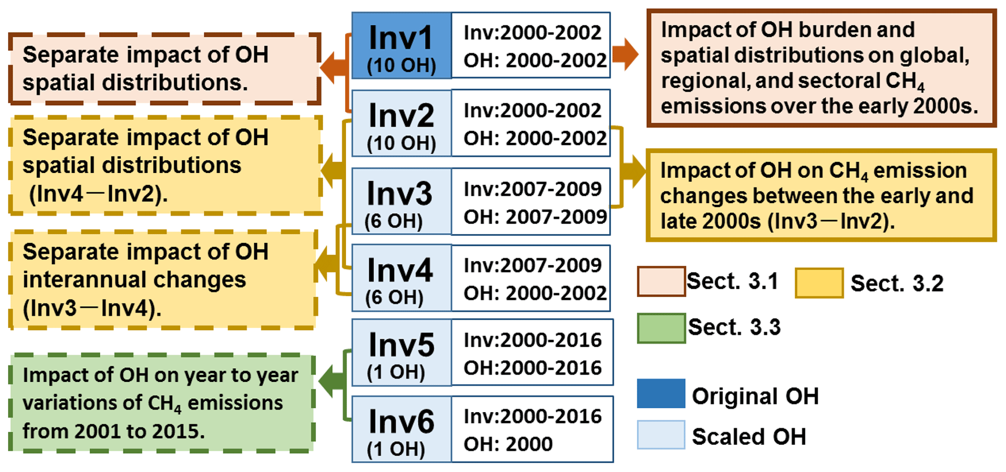
Figure 1A diagram showing inversion experiments (Inv1–Inv6) performed in this study. For each experiment, “Inv” gives the time period of inversion, and “OH” gives the time period of the OH fields used in the inversion. Inv1 is performed using the original OH field, whereas Inv2–Inv6 are performed using scaled OH fields. The colored boxes on the left and right show analyses of inversions we did to examine the OH impacts on inverted CH4 emissions. The brown, yellow, and green text boxes correspond to analyses presented in Sect. 3.1–3.3, respectively.
2.3 Model experiments
As shown in Fig. 1, we performed six groups of inversions (Inv1 to Inv6, 34 inversions in total). The impacts of OH on the top-down estimation of CH4 emissions are comprehensively analyzed by comparing the inversion results within one group or between two different groups. We analyze the overall impacts of differences in OH burden, spatial distribution, and temporal change on CH4 emissions (colored boxes on the right in Fig. 1) and separate the impacts of OH spatial distribution and temporal variations (colored boxes on the left in Fig. 1). The results are presented and discussed in three sections as shown in different colors in Fig. 1.
We perform four groups of 3-year CH4 inversion experiments using 6 to 10 OH fields (Inv1 to Inv4, Fig. 1) and two groups of 17-year CH4 inversions from 2000 to 2016 (Inv5 and Inv6, Fig. 1) using only CESM1-WACCM OH fields. For the short-term inversions, the first and last 6 months are treated as spin-up and spin-down periods and discarded from the following analyses (to avoid edge effect). Thus, we only analyze the results over July 2000–June 2002 (i.e., the early 2000s) for Inv1 and Inv2 and July 2007–June 2009 (i.e., the late 2000s) for Inv3 and Inv4. The early 2000s and the late 2000s represent the time periods with stagnant and resumed growth of atmospheric CH4 mixing ratios, respectively. For the long-term inversions, we take a 1-year spin-up and spin-down and analyze the 15-year results from 2001 to 2015.
The aim of Inv1, conducted for 2000–2002 with 10 OH fields, is to quantify the influence of both OH global burden and spatial distributions on top-down estimates of global, regional, and sectoral CH4 emissions (the brown box with the solid line, Fig. 1). Because of the long lifetime of CH4 relative to OH, the top-down estimates of regional CH4 emissions can be influenced by both global total OH burden and OH spatial and seasonal distributions. To separate the influence of OH spatial distributions (including their seasonal variations) from that of the global annual mean [OH], we conduct Inv2, wherein all the prescribed OH fields are globally scaled to the global [OH] value of the INCA NMHC OH field in 2000 to get the same loss of CH4 by OH (scaled OH fields). As such, Inv2 provides the uncertainty range of CH4 emissions induced by the OH spatial distribution in both the horizontal and vertical directions as well as seasonal variations when assuming that the global total burden of OH can be precisely constrained (the brown box with the dashed line, Fig. 1). Thus, Inv1 (the inversions using original OH fields) and Inv2 (the inversions using scaled OH fields) yield upper (uncertainties from both global OH burden and spatial distributions) and lower (uncertainties only from OH spatial and seasonal distributions) limits of the influences of OH on regional CH4 emissions, respectively.
To quantify the influence of OH on CH4 interannual emission changes, we also conduct Inv3 and Inv4 over 2007–2009, with six scaled OH fields (instead of 10 to limit computational time). While both of the inversions are done for 2007–2009 (Inv3 and Inv4), the OH variations during 2007–2009 (Inv3) and 2000–2002 (Inv4) are used for the two inversions, respectively. Therefore, the difference of Inv3–Inv2 reveals the impact of OH on CH4 emission changes between the early and late 2000s (the yellow box with solid lines in Fig. 1); Inv3–Inv4 separates the impact of OH interannual variations, and the difference of Inv4–Inv2 allows for the assessment of the uncertainties of optimized CH4 emission changes due to different OH spatial and seasonal distributions (the yellow boxes with dashed lines in Fig. 1).
Finally, we test the impact of OH year-to-year variations and trends on CH4 emissions over 2001–2015 by running two long-term inversions (Inv5 and Inv6) with the OH fields simulated by CESM-WACCM only (the green box with dashed lines in Fig. 1). Inv5 is forced by the OH fields with both year-to-year variations and trends, while Inv6 is forced by the OH fields for the year 2000. For each group, only one experiment was done for computational reasons. We chose OH fields simulated by CESM1-WACCM because they shows the largest year-to-year OH variations and a positive trend of 0.4 % yr−1 during 2000–2010 among the CCMI OH fields (Zhao et al., 2019). Therefore, inversions using CESM1-WACCM OH are expected to yield an upper limit of the influence of OH variations on CH4 emissions as seen from atmospheric chemistry models.
We evaluate the optimized CH4 emissions by comparing the simulated CH4 mixing ratios using prior and posterior CH4 emissions with independent measurements from the NOAA/ESRL Aircraft Project. The location of the observation site (Table S1 in the Supplement) and the vertical profile of the model bias in CH4 mixing ratios compared with the aircraft observations (model minus observations) are shown in the Supplement (Fig. S4a for Inv1 and Fig. S4b for Inv2). The comparisons with independent aircraft observations confirm the improvement of model-simulated CH4 mixing ratios when using posterior emissions. All of the inversions in Inv1 and Inv2 reach small biases when compared with aircraft observations (right panel of Fig. S4a and S4b), which means that it is hard to distinguish which OH spatial and vertical distributions are more realistic in terms of the quality of fit to these aircraft CH4 observations. For Inv1, the root mean square errors (, nobs is the number of observations) are reduced from up to more than 100 ppbv (prior) to ∼10 ppbv (posterior). For Inv2, although the CH4 mixing ratios simulated using prior emissions already match aircraft observations well (RMSE = 8–17 ppbv), the posterior emissions still reduce the RMSE by up to 10 ppbv.
In the following sections, to quantify uncertainties in top-down estimations of CH4 emissions due to OH, we calculate OH-induced CH4 emission differences and uncertainties as the standard deviation and the maximum minus minimum values of the inversion results, respectively.
3.1 The impacts of OH burden and spatial distributions on CH4 emissions in 2000–2002
3.1.1 Global total CH4 emissions
Based on the ensemble of the 10 different OH fields listed in Table 1, global total emissions inverted by our system in Inv1 vary from 518 to 757 Tg CH4 yr−1 during the early 2000s (July 2000–June 2002). The highest CH4 emissions exceeding 700 Tg yr−1 are calculated using MOCAGE and SOCOL3 OH fields, for which [OH] values (15.0×10⁵ and 16.3×10⁵ molec cm−3) are much higher than those of other OH fields (10.3–12.6×10⁵ molec cm−3), leading to a larger CH4 sink and as a consequence larger CH4 emissions due to the mass balance constraint of atmospheric inversions. The high [OH] values simulated by SOCOL3 and MOCAGE are mainly due to the high surface and mid-tropospheric NO mixing ratio simulated by these two models (Zhao et al., 2019). As analyzed in Zhao et al. (2019), the lack of N2O5 heterogeneous hydrolysis (by both SOCOL3 and MOCAGE) and the overestimation of tropospheric NO production by NO2 photolysis (by SOCOL3) are the major factors behind the overestimation of NO and OH.
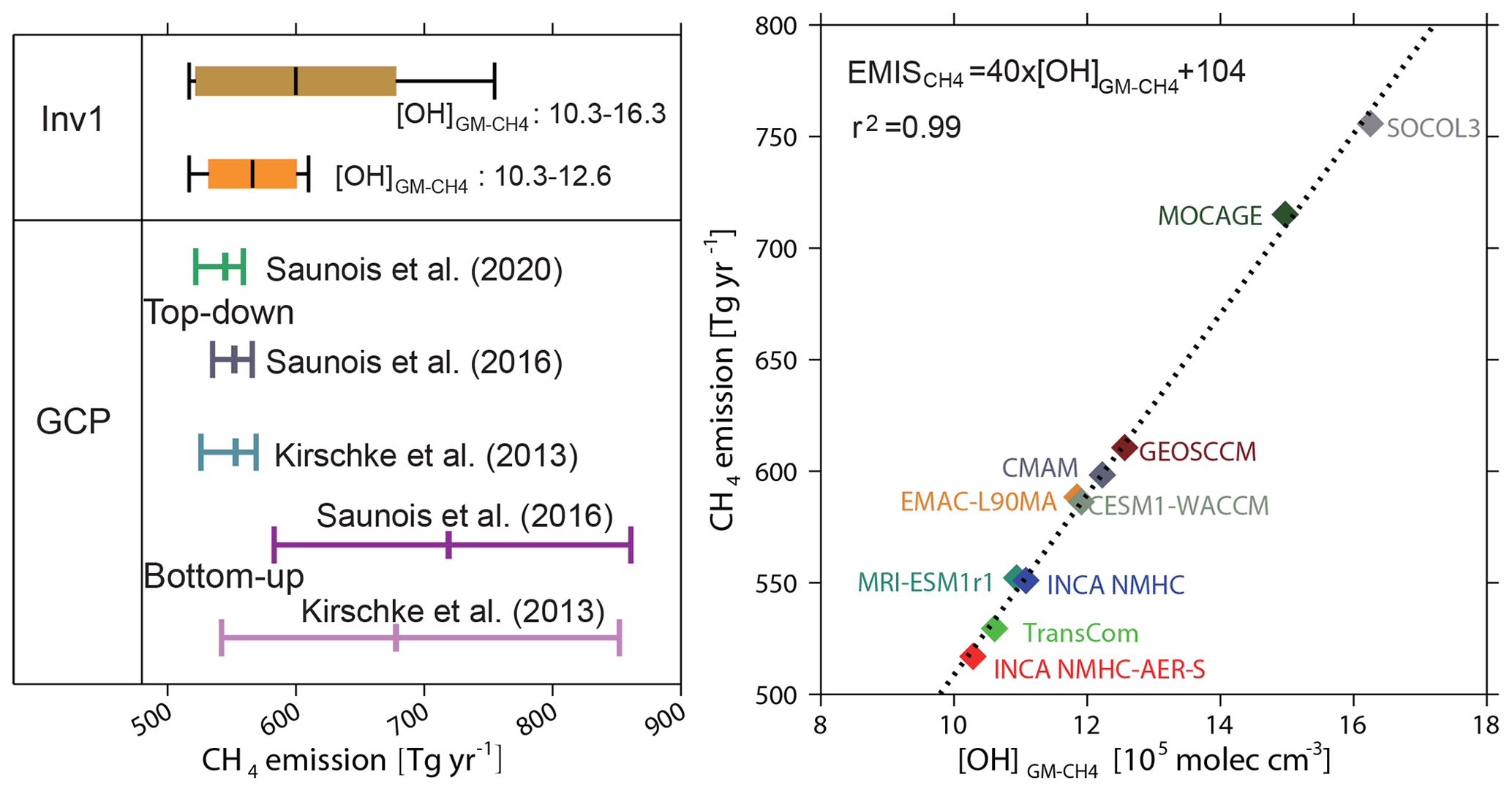
Figure 2(a) The global CH4 emissions from Inv1 (averaged over July 2000–June 2002). The bottom-up and top-down estimations over 2000–2009 from previous GCP calculations (Kirschke et al., 2013; Saunois et al., 2016, 2020) are also presented for comparison. The brown box plot shows the inversion results using 10 OH fields, while the orange one shows the results that exclude the largest estimates from the SOCOL3 and MOCAGE OH fields. The left, middle, and right whisker charts (vertical lines) represent the minimum, mean, and maximum values of different inversion, and the left and right edges of the boxes represent the mean ± 1 standard deviation. The definition of the box plot is applicable to all those hereafter. (b) The relationship between the optimized CH4 emissions (Tg yr−1) in Inv1 and the corresponding [OH] (×105 mole cm−3). The correlation coefficient (r) and the linear regression equation fitted to the data are shown in the inset.
Table 2The global total, hemispheric CH4 emissions, and interhemispheric difference of CH4 emissions calculated by Inv1 and Inv2 during the early 2000s (July 2000–June 2002; Tg yr−1).
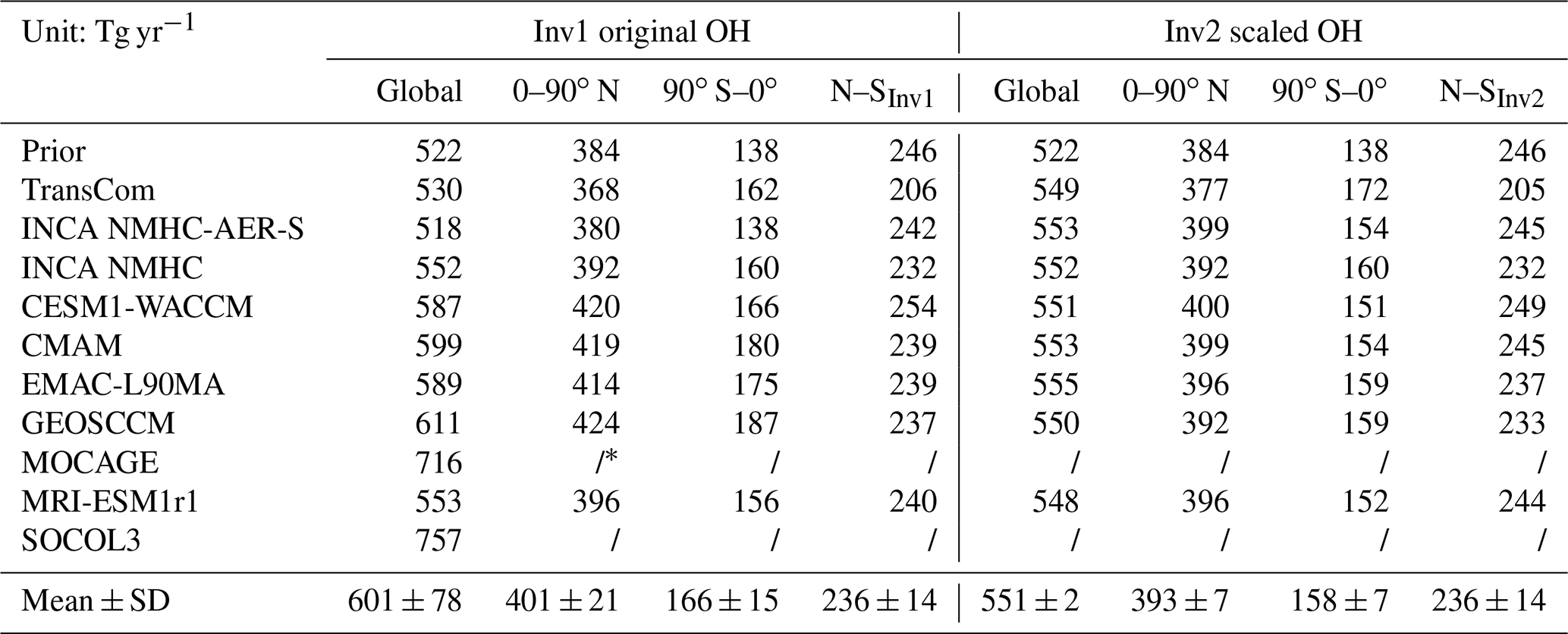
∗ We do not analyze the hemispheric CH4 emission estimated with the MOCAGE and SOCOL3 OH field since inversions using the two OH fields calculate much higher CH4 emissions than using other OH fields.
The minimum–maximum range of the CH4 emissions estimated by the 10 OH fields is almost similar to the range estimated by previous bottom-up studies (542–852 Tg yr−1 given by Kirschke et al., 2013, and 583–861 Tg yr−1 given by Saunois et al., 2016) from GCP syntheses and much larger than that reported by an ensemble of top-down studies for 2000–2009 in Kirschke et al. (2013) (526–569 Tg yr−1), Saunois et al. (2016) (535–566 Tg yr−1), and recent Saunois et al. (2020) (522–559 Tg yr−1) (Table 2 and Fig. 2). In the three top-down model ensembles, most of the inversion systems use TransCom OH fields, and the reported differences are mainly from different model transport and the setup of the inversion systems (e.g., the observations used in the inversions). Excluding the two outliers (MOCAGE and SOCOL-3) in Inv1, we find an uncertainty of about 17 % in global methane emissions (518 to 611 Tg yr−1) due to OH global burden and distributions, while transport model errors lead to only 5 % of the uncertainty of the global methane budget (Table 3; Locatelli et al., 2013). Our results indicate that considering different OH fields within top-down CH4 inversions would lead to larger uncertainty in the top-down CH4 budget.
Plotting top-down estimated CH4 emissions against [OH], which directly reflects the global OH oxidizing efficiency with respect to CH4 (Lawrence et al., 2001), reveals that the global total CH4 emissions vary linearly with [OH] (r2>0.99; Fig. 2b). The top-down estimation of global total CH4 emissions (EMIS) can be approximately calculated as
where a 1×10⁵ molec cm−3 (1 %) increase in [OH] will increase the top-down estimated CH4 emissions (EMIS) by 40 Tg yr−1, consistent with that given by He et al. (2020) using full-chemistry modeling and a mass balance approach. Other CH4 sinks including soil uptake and oxidation by O1(D), which are prescribed in this study, remove 104 Tg yr−1 of CH4. If uncertainties in all the CH4 sinks were also considered, the correlation between optimized CH4 emissions and the [OH] would be reduced. Using box model inversions, previous studies calculated that a 4 % (0.4×10⁵ molec cm−3) decrease in [OH]GM is equivalent to an increase of 22 Tg yr−1 of CH4 emissions (Rigby et al., 2017; Turner et al., 2017, 2019). If we apply the same [OH]GM changes in Eq. (1) (0.4×10⁵ molec cm−3), the equivalent emissions change is 16 Tg yr−1, about 25 % smaller than that given by Turner et al. (2017). This difference probably results from the different hemispheric mean reaction rates of OH+CH4 applied in box models, but it could also be due to different treatments of interhemispheric transport and stratospheric CH4 loss in global 3D transport models compared to simplified box models (Naus et al., 2019).
Table 3Global, latitudinal, and regional CH4 emissions (Tg yr−1; mean ± SD and the min–max range of the inversions) calculated by Inv1 and Inv2 during the early 2000s (July 2000–June 2002; Tg yr−1, excluding MOCAGE and SOCOL3). The uncertainties (unc. = (max–min) ∕ multi-inversion mean) arising from using different OH fields are compared with the uncertainties in CH4 emissions given by Saunois et al. (2016) and Locatelli et al. (2013).
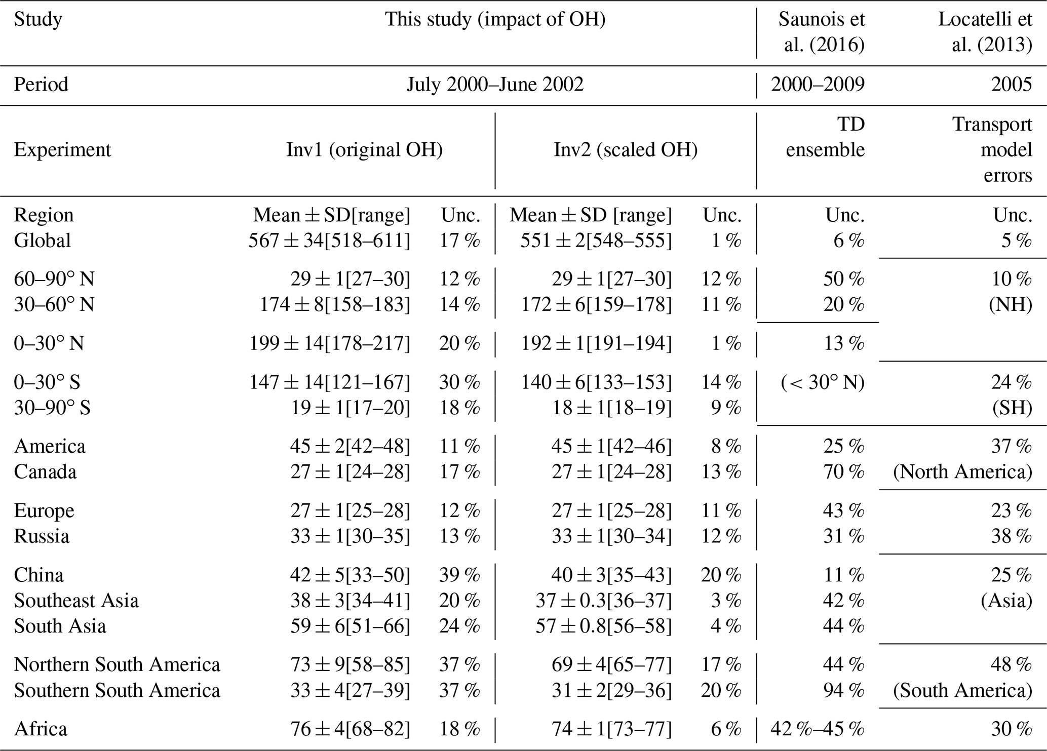
Table 4Global and latitudinal percentage changes in CH4-reaction-weighted [OH] from 2000–2002 to 2007–2009.

With the OH fields scaled to the same [OH] (11.1×10⁵ molec cm−3), the Inv2 simulations (assuming a global total OH burden that is well constrained) estimated global CH4 emissions of 551±2 Tg yr−1 (Table 3), as expected by the scaling. Differences in OH spatial distributions only lead to negligible uncertainty in global total CH4 emissions estimated by top-down inversions.
3.1.2 Regional CH4 emissions
Inv1 and Inv2
Since MOCAGE and SOCOL3 OH fields show much higher [OH]GM than constrained by MCF observations ( molec cm−3; e.g., Prinn et al., 2001; Bousquet et al., 2005) and give much higher estimates of CH4 emissions (>700 Tg yr−1) than other OH fields, we exclude inversion results with these two OH fields from the following analyses.
In response to both global total OH burden and interhemispheric OH ratios (Table 1), CH4 emissions over the Northern and Southern Hemisphere calculated by Inv1 (Table 2) vary from 368 to 424 Tg yr−1 (401±21 Tg yr−1) and 138 to 187 Tg yr−1 (166±15 Tg yr−1), respectively, resulting in a range in interhemispheric CH4 emission difference (NH-SH) of 206–254 Tg yr−1 (236±14 Tg yr−1). When scaling all OH fields to the same loss for Inv2, the standard deviations of hemispheric CH4 emissions are reduced to 7 Tg CH4 yr−1 for both hemispheres (Table 2), much smaller than those derived in Inv1 (21 and 15 Tg yr−1 over the Northern and Southern Hemisphere, respectively). However, the CH4 emission interhemispheric difference calculated by Inv2 remains at 236±14 Tg yr−1, similar to that calculated by Inv1, which indicates that the hemispheric CH4 emission differences are mainly determined by OH spatial distributions. Without the TransCom OH simulation, the interhemispheric CH4 emission difference ranges between 232 and 246 Tg yr−1. The TransCom OH field, for which the OH N∕S ratio is 1.0, leads to an interhemispheric CH4 emission difference of 205 Tg yr−1, which is 35 Tg yr−1 (27 Tg yr−1) smaller than the mean (minimum) interhemispheric difference calculated using other OH fields (OH N∕S ratio = 1.2–1.3). Previous studies show that differences in atmospheric transport models can lead to ±28 Tg yr−1 uncertainties in the top-down calculation of the interhemispheric CH4 emission difference using a single OH field – TransCom (Locatelli et al., 2013). Here, using a single atmospheric transport model but different OH fields, we find a ±14 Tg yr−1 uncertainty, which is about half of the atmospheric transport model uncertainty. Combining the two studies, one could expect more than 30 Tg yr−1 of uncertainty in top-down estimates of the interhemispheric CH4 emission difference based on different atmospheric models and different OH fields.
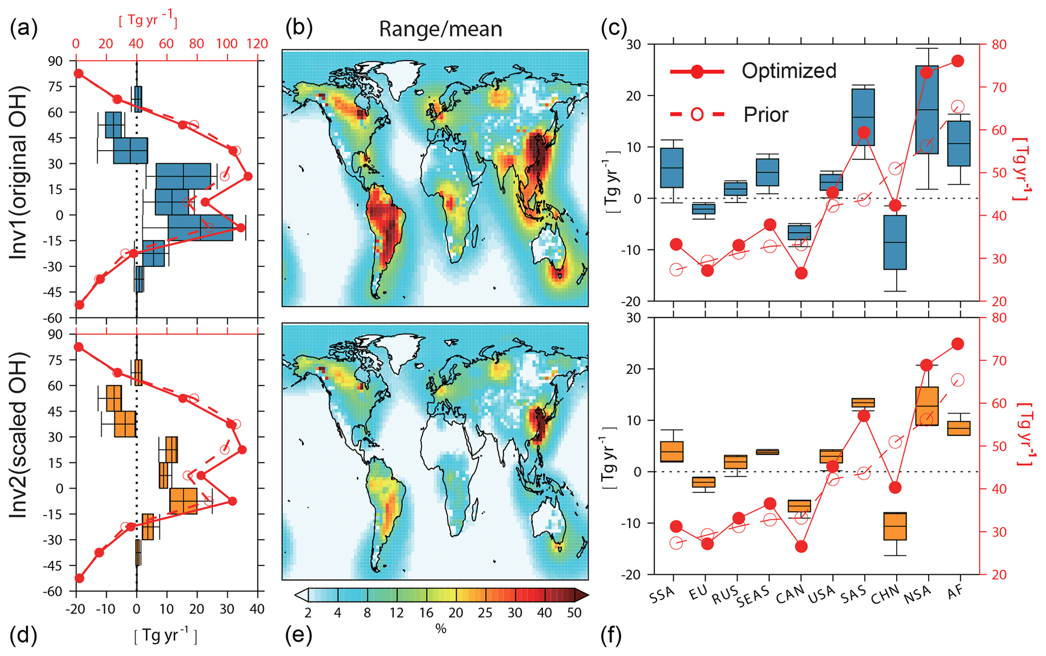
Figure 3Zonal (a, d), and regional averages (c, f) of CH4 emissions calculated by Inv1 (a, c) and Inv2 (d, f) with eight OH fields from July 2000–June 2002. (a, c, d, f) Prior (dashed red line) and mean optimized (solid red line) CH4 emissions for every 15∘ latitudinal band and 10 regions, respectively. USA: America, CAN: Canada, EU: Europe, RUS: Russia, CHN: China, SEAS: Southeast Asia, SAS: South Asia, NSA: northern South America, SSA: southern South America, AF: Africa. The full names of the abbreviations are applicable to all figures hereafter. The differences between prior and optimized emissions (optimized minus prior) are shown by the box plots (defined in Fig. 1). Prior and optimized emission values correspond to the right axes and their differences correspond to the left axes. (b, e) The ratio of the uncertainty range of emissions estimated with different OH fields (max–min) in each grid cell calculated by Inv1 (b) and Inv2 (e) to multi-inversion mean CH4 emissions.
Figure 3 shows the optimized and prior CH4 emissions calculated by Inv1 (a–c) and Inv2 (d–f) over latitudinal intervals (panels a, d) and large emitting regions (panels c, f). Compared with prior emissions, nearly all the optimized latitudinal and regional emissions show the same increment direction from prior emissions, but the magnitudes of the increment largely vary. The CH4 emissions calculated by Inv1 amount to (i) 147±14 Tg yr−1 and are 1–47 Tg yr−1 higher than the prior estimate over the southern tropical regions (30∘ S–0∘), (ii) 199±14 Tg yr−1 and are 6–45 Tg yr−1 higher than the prior estimate over the northern tropical regions (0–30∘ N), and (iii) 174±8 Tg yr−1 and are 1–26 Tg yr−1 lower than the prior estimate over the northern midlatitude regions (30–60∘ N) (Table 3). The uncertainties in global OH burden and distributions lead to larger uncertainty (maximum–minimum) in top-down estimated CH4 emissions over the tropics (>20 % of multi-inversion mean) and smaller uncertainty over the northern midlatitude regions (14 %) compared with that arising from transport model errors and different observations given by Saunois et al. (2016) (13 % over the tropics and 20 % over northern midlatitude regions) (Table 3).
Over the large emitting regions Europe (EU), Canada (CAN), and China (CHN), optimized emissions are lower than the prior. The emissions calculated by Inv1 show the largest absolute OH-induced differences over South America (SA, 73±9 Tg yr−1), South Asia (SAS, 59±6 Tg yr−1), and China (42±5 Tg yr−1) (Fig. 3c, f and Table 3), of which the uncertainty (maximum-minimum) accounts for more than 20 % of the multi-inversion mean emission over the corresponding regions (Table 3). Over high-latitude regions (Canada, Europe, and Russia), OH leads to small uncertainty ranges (<10 Tg yr−1). At the model grid scale, the uncertainty range due to OH can be much larger than the regional mean (Fig. 3b, e): for example, larger than 50 % of the multi-inversion mean emissions over South America and East Asia. As shown in Table 3, at regional scales, the uncertainty (maximum-minimum) in top-down estimated CH4 emissions due to different OH global burden and distributions over Asia and South America (∼37 % of multi-inversion mean) are of the same order as those arising from transport errors (25 % and 48 %) or given by Saunois et al. (2016) (∼40 %). Over other regions, using different OH fields leads to smaller uncertainties (11 %–18 %) compared to other causes of errors (23 %–70 %) (Table 3).
The uncertainties in the top-down estimated regional emissions are not only due to inter-model differences of the regional OH fields but also rely on the distribution of the surface observations used in the inversions. Over the regions with large prior emissions but less constrained by observations (e.g., South America, South Asia, and China), our OH analysis leads to larger uncertainties than regions that are well constrained by observations (e.g., the North America and Canada) (Fig. S3). The results may indicate that on the regional scale, the top-down estimated CH4 emissions and the uncertainties arising from OH are specific to the observation system retained. If more surface observations (e.g., in the Southern Hemisphere) or satellite columns with a more even global coverage were included in our inversions, spatial patterns of the top-down estimated CH4 emissions and their uncertainties (as shown by Fig. 3) could be different.
Comparing Inv1 and Inv2
We now compare the inversion results using the original OH fields (Inv1) with those using scaled OH fields (Inv2) to estimate how much the optimized regional CH4 emission differences of Inv1 are dominated by OH spatial and seasonal distributions versus the global OH burden. Applying one single global scaling factor per model reduces the inter-model differences of original OH fields by 33 %, 67 %, and 33 % in the southern tropics (0–30∘ S), northern tropics (0–30∘ N), and northern middle and high latitudes (30–90∘ N) (Table S2). This scaling results in a 57 %, 93 %, and 22 % reduction of OH-induced latitudinal CH4 emission differences, respectively, for the southern tropics (0–30∘ S), northern tropics (0–30∘ N), and northern middle and high latitudes (30–90∘ N) (Fig. 3a, d comparing standard deviations of Inv1 and Inv2). At the regional scale (Fig. 3c, f and Table 3), the OH spatial-distribution-induced CH4 emission differences (standard deviation of Inv2) account for 50 % of the differences due to both OH burden and spatial distributions (standard deviation of Inv1) over northern midlatitude regions (China, North America) and South America. Over northern tropical regions (southern Asia and Southeast Asia), the OH spatial distribution induces negligible CH4 emission differences.
The comparison of Inv1 and Inv2 reveals that methane emissions in tropical regions are less sensitive to OH spatial distribution than middle- and high-latitude regions in our framework. One possible explanation could be the location of monitoring sites. Over tropical regions, CH4 emissions are less constrained (with few to no observation sites near source regions) than in the northern extratropics, where several monitoring sites are located at or near regions with high CH4 emission rates and high OH uncertainties (e.g., North America, Europe, and downwind of East Asia). Thus, CH4 emissions over the tropical regions mainly contribute to matching the global total CH4 sinks (instead of the sinks over the tropical regions only) estimated by inversion systems. When all OH fields are scaled to the same CH4 losses (Inv2), differences in emissions over the tropical regions are therefore largely reduced.

Figure 4Global total CH4 emissions from four broad categories from July 2000–June 2002 (Tg yr−1). The red circles and dots show the prior emissions and mean optimized emissions, respectively, as calculated by Inv1 (right axes), and the box plots (defined in Fig. 1) show the difference between prior emissions (optimized minus prior, left axes) and optimized emissions calculated by Inv1 (blue) and Inv2 (yellow).
3.1.3 Global and regional CH4 emissions per source category
Figure 4 compares optimized and prior global total CH4 emissions and the difference between the prior and optimized CH4 emissions for four broad source categories: wetlands, agriculture and waste (called agri-waste), fossil fuels, and other natural sources. We attribute the optimized emissions to different source sectors depending on the relative strength of individual prior sources in each grid cell. With original OH fields, Inv1 calculates CH4 emissions of 203±15 Tg yr−1 for wetlands, 209±12 Tg yr−1 for agri-waste, 89±4 Tg yr−1 for fossil fuel, and 66±3 Tg yr−1 for other natural sources. Optimized emissions of the four sectors are 23±15 Tg yr−1 (−2–42 Tg yr−1), 13±12 Tg yr−1 (−3–29 Tg yr−1), 5±4 Tg yr−1 (−1–9 Tg yr−1), and 4±3 Tg yr−1 (0–8 Tg yr−1) higher than the prior emissions, respectively. Although Inv2 is conducted with scaled OH fields and all inversions calculate similar global total CH4 emissions (551±2 Tg yr−1), optimized CH4 emissions still show some uncertainties due to OH (as a standard deviation) (3 Tg yr−1 for wetland emissions and 2 Tg yr−1 for agriculture and waste; yellow box plots in Fig. 4) in response to different OH spatial distributions.

Figure 5Same as Fig. 4 but for prior and optimized emissions over 10 emitting regions covering most of the emitting lands. W: wetlands, A: agri-waste, F: fossil fuels, and O: others (Tg yr−1).
We have further calculated CH4 emissions per source category and per region estimated by Inv1 (Fig. 5) to explore the contribution of each region to the OH-induced sectoral emission uncertainties. Wetland CH4 emissions mainly dominate emissions over northern South America, Africa, South and East Asia, and Canada. Northern South America (53±7 Tg yr−1) and Africa (30±2 Tg yr−1) contribute most of the global total OH-induced wetland emission differences and are 1–22 Tg yr−1 and 1–8 Tg yr−1 higher than prior emissions, respectively. In contrast to the higher wetland emissions than prior ones over tropical regions, optimized boreal wetland emissions (in Canada) are 6–9 Tg yr−1 lower than prior emissions, consistent with lower top-down estimations than the prior given by Saunois et al. (2016). Agriculture and waste emissions are most intensive over China (25±3 Tg yr−1) and South Asia (SAS) (39±3 Tg yr−1). The optimized inventories show lower agriculture and waste emissions over China (0.6–10 Tg yr−1) and Europe (1–3 Tg yr−1) and much higher emissions over SAS (4–13 Tg yr−1) compared with the prior emission inventory. The OH-induced differences in fossil fuel emissions are found mainly in China and Africa, which are 0.8–5 Tg yr−1 lower and 0.6–3 Tg higher than prior emissions, respectively. In agreement with the previous regional discussion, scaling OH (Inv2) highly reduces the uncertainties attributable to different OH over the tropical regions but not for the middle- to high-latitude regions. In Inv2, the largest CH4 emission differences due to different OH spatial distributions are found for wetland emissions in South America (60±4 Tg yr−1), agriculture and waste emissions in South Asia (17±1 Tg yr−1) and China (24±2 Tg yr−1), and fossil fuel emissions in China (8±0.7 Tg yr−1) and Russia (9±0.4 Tg yr−1).
Previous studies have highlighted the fact that anthropogenic emissions over China are largely overestimated by bottom-up emissions inventories compared with top-down estimates (Kirschke et al., 2013; Tohjima et al., 2014; Saunois et al., 2016). In our study, total anthropogenic emissions (agriculture, waste, and fossil fuel) over China are 1–15 Tg yr−1 lower than the prior bottom-up inventory as calculated by Inv1 and 7–14 Tg yr−1 as calculated by Inv2, with the lowest emissions calculated with the TransCom OH field (for both Inv1 and Inv2). The TransCom OH field is the most widely used in current top-down CH4 emission estimations but shows much lower [OH] over China than other OH fields (Zhao et al., 2019), which may be due to the use of the same NOx profile over East Asia as for remote regions based on observations of the 1990s when constructing the TransCom OH field (Spivakovsky et al., 2000). Thus, the large reduction of top-down estimated anthropogenic CH4 emissions over China compared to the prior emissions may be partly due to an underestimation of [OH] over China in the TransCom field.
Table 5Global total emission changes (Tg yr−1) from the early 2000s (July 2000–June 2002) to the late 2000s (July 2007–June 2009) calculated to identify the effect of OH fields (Inv3–Inv2), the effect of OH fixed to the early 2000s (Inv4–Inv2), and the contribution of OH changes from the early to late 2000s to top-down estimated CH4 emissions changes (Inv3–Inv4).
3.2 Impact of OH on CH4 emission changes between 2000–2002 and 2007–2009
As shown in Table 4, the global mean [OH] simulated by CCMI models increased by 0.7 %–1.8 % from 2000–2002 to 2007–2009 in response to anthropogenic emissions and climate change (Zhao et al., 2019), whereas the INCA-NMHC model-simulated global [OH] shows a slight decrease of 0.5 %. The TransCom OH field, being constant over time, shows no change. The increase in global mean [OH] mainly results from the combination of a higher increase in the tropics compared to the northern extratropics and a slight decrease in the southern extratropics. As a result, the changes in OH between the two periods show different patterns between regions. We have conducted inversions for 2007–2009 with scaled OH fields (Inv3) to explore how uncertainties in OH (both the spatial and seasonal distribution and interannual changes) can influence the top-down estimates of temporal CH4 emission changes from the early 2000s (July 2000–June 2002, Inv2) to the late 2000s (July 2007–June 2009, Inv3) (Inv3-Inv2). We have also performed Inv4 for 2007–2009 but using OH fields of 2000–2002 to separate the contribution of OH from different time periods (Inv3-Inv4).
3.2.1 Global total emission changes between 2000–2002 and 2007–2009
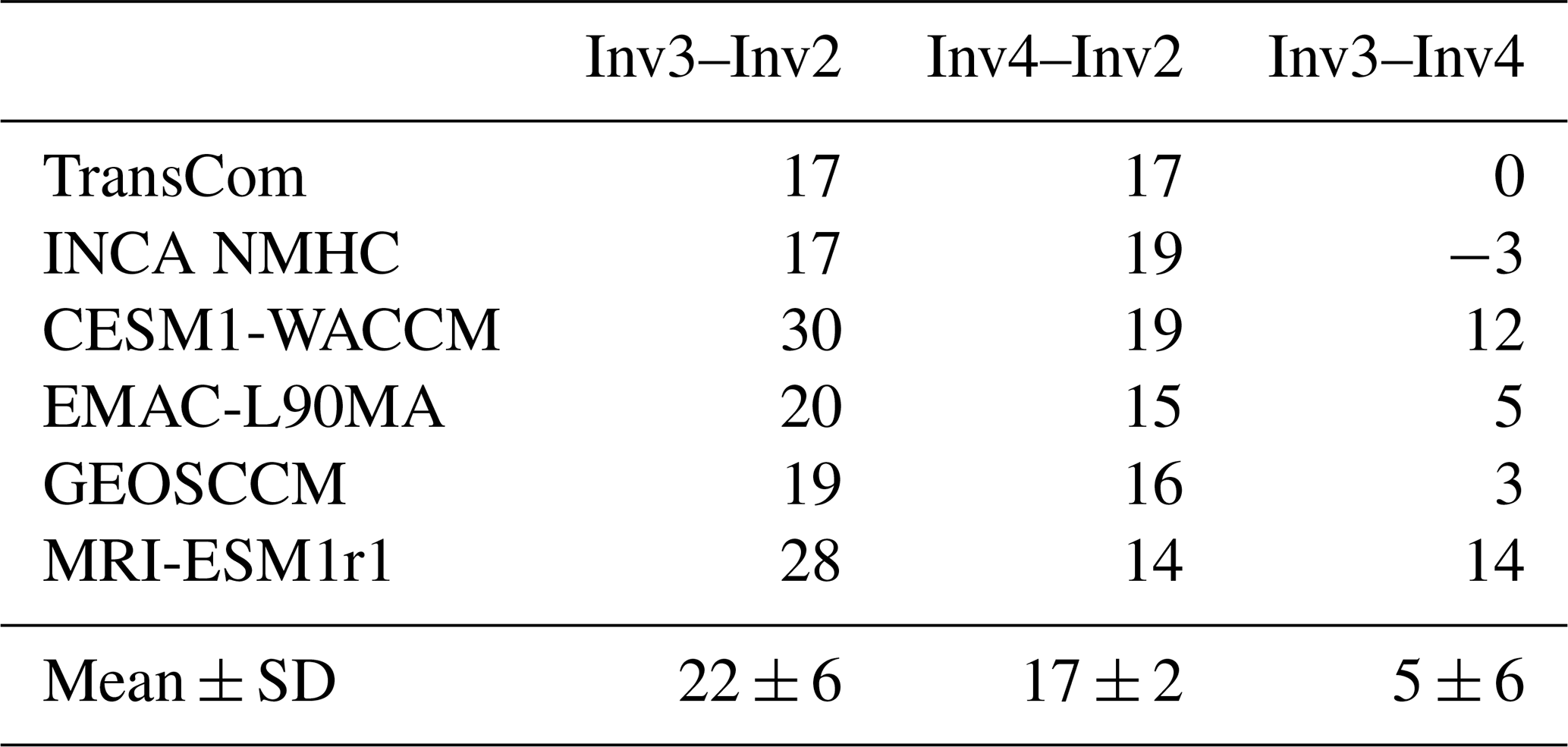
Total emission changes. From the early 2000s (Inv2) to the late 2000s (Inv3), the top-down estimated CH4 emissions increased by 22±6 Tg yr−1 (17–30 Tg yr−1; Table 5). The largest CH4 increase of 30 Tg yr−1 is estimated with CESM1-WACCM OH fields (for which OH increased by 1.8 % from 2000–2002 to 2007–2009), 13 Tg yr−1 higher than the smallest increase of 17 Tg yr−1 estimated with the INCA NMHC OH field (for which OH decreased by 0.5 % from 2000–2002 to 2007–2009). In Saunois et al. (2017), the minimum–maximum uncertainty range of emission changes between 2002–2006 and 2008–2012 was 16 Tg yr−1. This means that the uncertainty attributable to uncertainty in OH fields (13 Tg yr−1) is comparable to the minimum–maximum uncertainty resulting from using different atmospheric chemistry–transport models and observations (surface and satellite) but mostly constant OH over time (16 Tg yr−1; Saunois et al., 2017).
Spatial versus temporal OH effects. Only changing OH from 2000–2002 (Inv4) to 2007–2009 (Inv3), top-down estimated CH4 emissions due to OH interannual changes are 5±6 Tg yr−1 (−3–14 Tg yr−1; Table 5), which contribute 25 % of total optimized emission changes (Inv3-Inv2) between the early and late 2000s (22±6 Tg yr−1; Table 5). As listed in Table 5, the largest emission increases due to OH interannual changes are calculated using MRI-ESM1r1 OH fields, for which a 1.1 % global increase in OH can up to double the top-down estimation of CH4 emission increase from the early to the late 2000s. This result indicates that a large bias likely exists in the former top-down estimation of the CH4 emission trend calculated without considering OH changes (Saunois et al., 2017).
Keeping OH fields for 2000–2002, top-down estimated CH4 emissions increase by 17±2 Tg yr−1 (14–19 Tg yr−1; Table 5) between the early 2000s (Inv2) and the late 2000s (Inv4) in response to increasing atmospheric CH4 mixing ratios and temperature. This represents 75 % of total optimized emission changes (Inv3-Inv2) between the early and late 2000s (22±6 Tg yr−1; Table 5). The 2 Tg yr−1 uncertainty (as a standard deviation) is due to the different OH spatial and seasonal distributions, indicating that OH spatial and seasonal distributions, which are not considered in box models, can also contribute to the uncertainties in optimized CH4 emission changes.
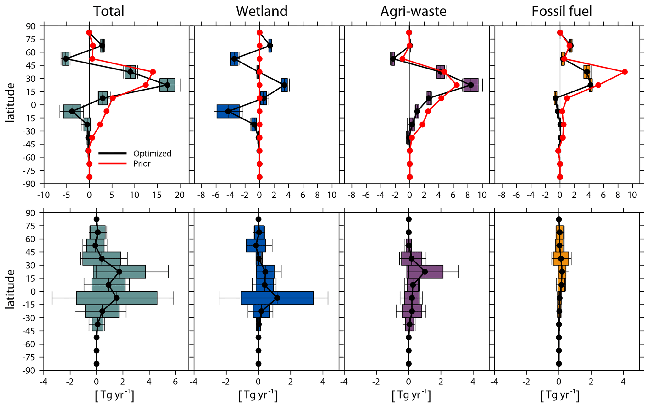
Figure 6Top: latitudinal emission (every 15∘ latitudinal band) changes (Tg yr−1) from the early 2000s (July 2000–June 2002) to the late 2000s (July 2007–June 2009) in total, wetlands, agriculture and waste, and fossil fuel emissions (Inv3-Inv2). Bottom: contribution of OH changes to top-down estimated CH4 emission changes between the two periods (Inv3-Inv4). The red lines are changes in prior emissions, and the black lines are the mean changes in optimized emissions. The box plots (defined by Fig. 1) show the standard deviations and ranges calculated with different OH fields.
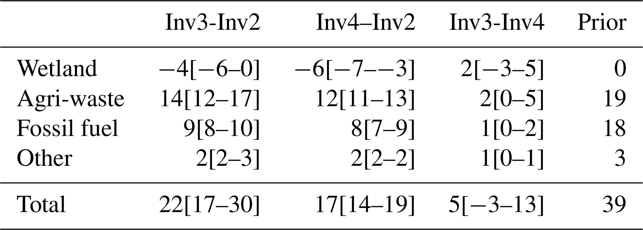
Table 6Global sectoral emission changes (Tg yr−1) from the early 2000s (July 2000–June 2002) to the late 2000s (July 2007–June 2009) (mean and the min–max range).
3.2.2 Emission changes by source type and region
Total emission changes. We further analyze the influence of OH (both spatial distributions and interannual variations) on the top-down estimated sectoral and regional CH4 emission changes from the early 2000s (Inv2) to the late 2000s (Inv3). As shown in Fig. 6 (top panels), the smaller increase in the optimized global CH4 emissions from the early 2000s to the late 2000s (17–30 Tg yr−1) compared to the prior change (39 Tg yr−1) is mainly due to a decrease in wetland emissions over the southern tropics (3–6 Tg yr−1, 15–0∘ S) and northern midlatitude regions (3–4 Tg yr−1, 45–60∘ N) in contrast to the climatology of prior wetland emissions and a lower fossil fuel emission increase over 30–45∘ N (3–4 Tg yr−1) compared to prior emission increase (9 Tg yr−1). Wetlands (−6–0 Tg yr−1) as well as agriculture and waste (12–17 Tg yr−1) contribute most of the total OH-induced uncertainty in global total emission changes (17–30 Tg yr−1) from the early 2000s (Inv2) to the late 2000s (Inv3) (Table 6), whereas fossil fuel emissions (8–10 Tg yr−1) show smaller uncertainty.
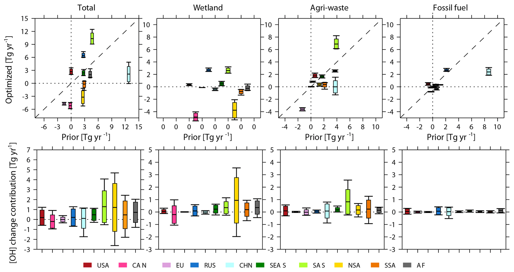
Figure 7Top: optimized global total and sectoral regional emission changes (Tg yr−1) from the early 2000s to the late 2000s (y axis) plotted against prior emission changes between the two time periods (x axis) as derived from Inv2 and Inv3. The prior wetland emissions are constant over time and thus show zero changes (all “0” on the x axis). Bottom: contribution of OH changes between the two periods to top-down estimated emission changes (Inv3-Inv4). The box plots (defined by Fig. 1) show the standard deviations and ranges calculated with different OH fields.
Considering emissions over latitudinal bands (Fig. 6, top panels), the largest spread of emission changes is found over the southern tropics (15∘ S – tropics, −7 to −1 Tg yr−1), northern subtropics (15–30∘ N, 16 to 20 Tg yr−1), and northern extratropical regions (30–45∘ N, 8 to 11 Tg yr−1). The spread over the southern tropics is dominated by emission changes from wetlands (−6 to −2 Tg yr−1), over northern subtropics by agriculture and waste (7 to 10 Tg yr−1), and over northern extratropical regions by agriculture and waste (4 to 5 yr−1) and fossil fuels (3 to 4 Tg yr−1). At the regional scale (Fig. 7, top panels), northern South America (−5 to −1 Tg yr−1), South Asia (9 to 12 Tg yr−1), and China (0 to 5 Tg yr−1) show the largest differences in emission changes from the early 2000s to the late 2000s. The multi-inversion calculated agriculture and waste sector emission changes in China disagree in sign (Fig. 7; top panels), which range from a 1 Tg yr−1 decrease to a 2 Tg yr−1 increase from the early 2000s to the late 2000s.
We now compare the uncertainty of top-down estimated CH4 emission changes from the early to the late 2000s due to different OH spatial–temporal variations with the ensemble of top-down studies given by Saunois et al. (2017). For the sectoral emissions, emission changes from agriculture and waste as well as from wetlands show the largest uncertainties (more than 50 % of the multi-inversion mean; Inv3-Inv2 in Table 6) induced by OH spatial–temporal variations, comparable to those given by Saunois et al. (2017). On the contrary, the uncertainty of fossil fuel emission changes (24 % of the multi-inversion mean) is much smaller than that given by Saunois et al. (2017). For regional CH4 emission changes, the uncertainty induced by OH spatial–temporal variations is usually larger than the multi-inversion mean emission changes (except South Asia) and similar to that given by Saunois et al. (2017). The large differences in different top-down estimated regional and sectoral emission changes are mainly attributed to model transport errors in Saunois et al. (2017). Here, our results show that uncertainties due to OH spatiotemporal variations can lead to similar biases in top-down estimated CH4 emission changes.
Spatial versus temporal effects. We now separate the influences of OH interannual changes (Inv3-Inv4) on optimized regional CH4 emission changes. As shown in the bottom panels of Figs. 6 and 7, at the regional scale, OH interannual changes mainly perturb top-down estimated CH4 emission changes over the southern tropics (0–15∘ S, −3–6 Tg yr−1) and northern subtropics (15–30∘ N, 0–5 Tg yr−1). This corresponds to the two largest spreads observed in Fig. 7 associated with wetland emissions over northern South America (−2–4 Tg yr−1) and with agriculture and waste emissions over South Asia (0–3 Tg yr−1). Among the four emission sectors, wetland emissions (mainly southern tropical wetland) show the largest change (−3–5 Tg yr−1) in response to OH temporal changes (Table 6), which account for 60 % of total wetland emission changes between these two periods.
The OH spatial and seasonal distribution can lead to large uncertainties in regional CH4 emission changes. For regional and latitudinal scales, the spreads (uncertainty ranges) of Inv4-Inv2 (OH fixed to 2000–2002) (Figs. S5 and S6) are comparable to the spread of regional and latitudinal emission changes arising from both OH interannual changes and spatial and seasonal distributions (Inv3-Inv2) (top panels of Figs. 6 and 7) as mentioned above (e.g., a 3–5 Tg yr−1 decrease over northern South America, a 6–11 Tg yr−1 increase over South Asia, and a 0–4 Tg yr−1 increase over China). These results show that even if the global total OH burden is well constrained (as in Inv4 and Inv2, wherein all OH fields are scaled to the same [OH], and the differences in optimized CH4 emission changes from the early 2000s to the late 2000s are only due to different OH spatial distributions), top-down estimates of sectoral and regional temporal CH4 emission changes remain highly uncertain.
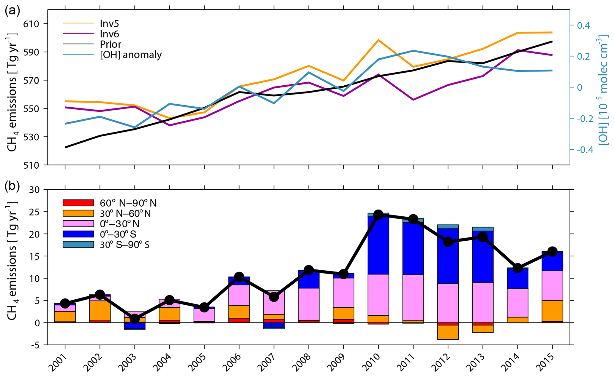
Figure 8(a) Time series of global total CH4 emissions calculated by Inv5 (yellow) and Inv6 (purple) plotted together with prior emissions (black) and the [OH] anomaly of CESM OH fields (blue). (b) The difference in global total (black line) and latitudinal (stack bar plots) CH4 emissions between Inv5 and Inv6 (Inv5–Inv6).
3.3 Impacts of OH on year-to-year variations of CH4 emissions from 2001 to 2015
To infer the influence of OH year-to-year variations on top-down optimized long-term CH4 emission changes, we conducted two inversions, Inv5 and Inv6. Inv5 calculates optimized CH4 emissions from 2001 to 2015 with the CESM1-WACCM OH field varying from one year to the next, while Inv6 uses the CESM1-WACCM OH field but fixed to the year 2000. The choice of the CESM1-WACCM OH field is explained in Sect. 2.3 above. As shown in Fig. 8, the [OH] of the CESM1-WACCM OH field increases by 0.47×10⁵ molec cm−3 (4.2 %) from 2001 to 2011 and then decreases by 0.13×10⁵ molec cm−3 (1.1 %) from 2011 to 2015.
With OH fixed to the year 2000 (Inv6), global CH4 emissions stall at 550±2 Tg yr−1 during 2001–2003 and decrease to 538 Tg yr−1 in 2004, which is different from the continuous increase in CH4 emissions given by the bottom-up inventory (Fig. 8a). After 2004, global total CH4 emissions show a positive trend of 3.5±1.8 Tg yr−2 (P<0.05) but smaller than the prior bottom-up inventory (4.3±0.6 Tg yr−2; P<0.05). Both stalled and decreased emissions during 2001–2004 as well as the increasing trend after 2004 are consistent with previous top-down estimations (Saunois et al., 2017).
The trend of global CH4 emissions during 2004–2016 calculated by Inv5 (using varying OH) is 4.8±1.8 Tg yr−2 (P<0.05), which is 1.3 Tg yr−2 (36 %) higher than that calculated by Inv6 (OH fixed to 2000) due to the small increase in [OH] and also 0.5 Tg yr−2 higher than the prior emission trend (4.3±0.6 Tg yr−2). Accounting for the OH increasing trend leads to increasing the prior trend in Inv5 instead of decreasing it in Inv6. When calculating the differences between Inv5 and Inv6 for different latitude intervals, we find that before 2004, differences between Inv5 and Inv6 are mainly contributed by northern middle-latitude regions, whereas after 2004 they are dominated by tropical regions (Fig. 8b).
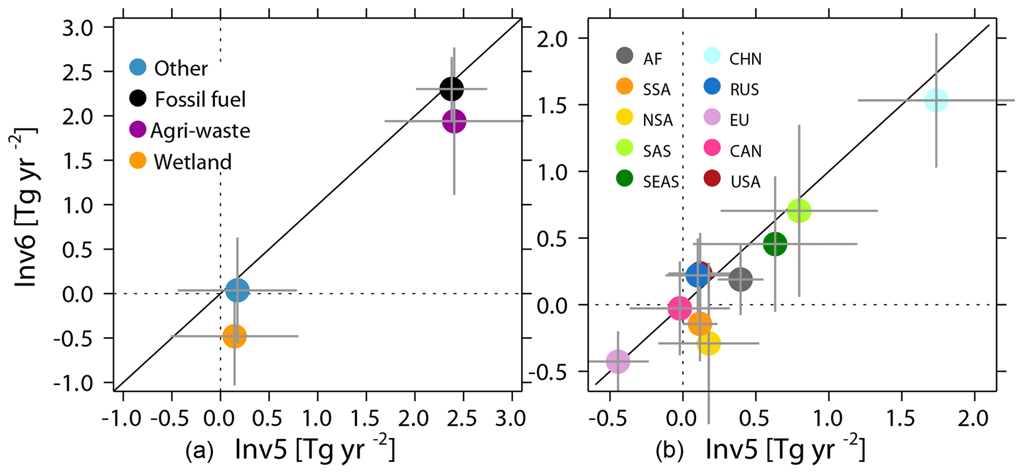
Figure 9Comparison between Inv5 (x axis) and Inv6 (y axis) estimated global total CH4 emissions trends (Tg yr−2) between 2004 and 2015 for the four categories (a) and over the 10 continental regions (b). The error bars show the trend with 95 % confidence intervals.
We further compare CH4 emission trends for the four previously defined emission sectors and the 10 continental regions between Inv5 and Inv6. As shown in Fig. 9, the positive global CH4 emission trend during 2004–2016 is mainly contributed by anthropogenic sources from agriculture and waste, as well as fossil-fuel-related activities, which are 1.9±0.7 Tg yr−2 and 2.3±0.4Tg yr−2, respectively, as calculated by Inv6 (fixed OH). Wetland emissions show a small negative trend ( Tg yr−2), and other natural emissions do not show a significant trend (0.04±0.6 Tg yr−2). Both sectors show large uncertainties in their trends, reflecting large year-to-year variations. When considering [OH] variations, Inv5 estimates a higher agriculture and waste emission trend (2.4±0.8 Tg yr−2) compared to Inv6, mainly contributed by China (1.5±0.5 Tg yr−2 for Inv6 versus 1.7±0.5 Tg yr−2 for Inv5) and southern South America ( Tg yr−2 for Inv6 versus 0.1±0.3 Tg yr−2 for Inv5). Accounting for interannual OH variations, the negative wetland emission trend reduces to near zero (0.1±0.6 Tg yr−2), mainly due to increased emission trends over northern South America ( Tg yr−2 for Inv6 versus 0.2±0.5 Tg yr−2 for Inv5). In contrast to agriculture and waste as well as wetland emissions, fossil fuel emissions have a similar positive trend of 2.4±0.4 Tg yr−2 in Inv5 and Inv6. This result comes from a higher CH4 emission trend over China calculated by Inv5 balanced by a lower CH4 emission trend over America and Russia (0.2±0.2 Tg yr−2 for Inv6 versus 0.1±0.3 Tg yr−2 for Inv5) since the CESM1-WACCM OH field shows a significant negative [OH] trend over America (Zhao et al., 2019).
In this study, we have performed six groups of variational Bayesian inversions (top-down, 34 inversions in total) using up to 10 different prescribed OH fields to quantify the influence of OH burden, interannual variations, and spatial and seasonal distributions on the top-down estimation of (i) global total, regional, and sectoral CH4 emissions, (ii) emission changes between the early 2000s and late 2000s, and (iii) year-to-year emission variations. Our top-down system estimates monthly CH4 emissions by assimilating surface observations with atmospheric transport of CH4 calculated by the offline version LMDz5B of the LMDz atmospheric model using different prescribed OH fields.
Based on the ensemble of 10 original OH fields ([OH]:10.3–16.3×10⁵ molec cm−3), the global total CH4 emissions inverted by our system vary from 518 to 757 Tg yr−1 during the early 2000s, similar to the CH4 emission range estimated by previous bottom-up syntheses and larger than the range reported by top-down studies (Kirschke et al., 2013; Saunois et al., 2016, 2020). The top-down estimated global total CH4 emission varies linearly with [OH], which indicates that at the global scale, a small uncertainty of 1×10⁵ molec cm−3 (10 %) [OH] can result in 40 Tg yr−1 uncertainties in optimized CH4 emissions.
At the regional scale (excluding the two highest OH fields), CH4 emission uncertainties due to different OH global burdens and distributions are largest over South America (37 % of multi-inversion mean), South Asia (24 %), and China (39 %), resulting in significant uncertainties in optimized emissions from the wetland as well as agriculture and waste sectors. These uncertainties are comparable in these regions with those due to model transport errors and inversion system setup (Locatelli et al., 2013; Saunois et al., 2016). For these regions, the uncertainty due to OH is critical for understanding their methane budget. In other regions, OH leads to smaller uncertainties compared to that given by Locatelli et al. (2013) and Saunois et al. (2016). By performing inversions with globally scaled OH fields, we calculated that emission uncertainties due to different OH spatial and seasonal distributions account for ∼50 % of total uncertainties (induced by both different OH burdens and different OH spatial and seasonal distributions) over middle- to high-latitude regions and South America. CH4 emission differences due to OH spatial distributions are the largest in northern South America and China but are negligible over South Asia and other northern tropical regions. Based on CH4 emission optimization with surface observations, our study shows that tropical regions appear to be more sensitive to the OH global burden (as less constrained regions used to achieve the global mass balance of the methane budget), and middle- to high-latitude regions are found to be sensitive to both the OH global burden and spatial distributions.
The global CH4 emission change between 2000–2002 and 2007–2009 as estimated by top-down inversions using six different OH fields is 22±6 Tg yr−1, of which 25 % (5±6 Tg yr−1) is contributed by OH interannual variations (mainly by an increase in [OH]), while 75 % can be attributed to emission changes resulting from the increase in observed CH4 mixing ratios and atmospheric temperature (considering constant OH). Among the four emission sectors, wetland emissions (mainly southern tropical wetlands) show the largest change of 2±3 Tg yr−1 in response to OH temporal changes, which account for 60 % of total wetland emission changes between these two periods. For global total emission changes, OH spatial distributions lead to lower uncertainties than interannual variations (2 Tg yr−1 versus 6 Tg yr−1), but at the regional scale, OH spatial distributions and interannual variations are of equal importance for quantifying CH4 emission changes.
As the modeled OH used here mainly shows an increase in [OH] (meaning an increasing CH4 sink) during the 2000s, our inversion using year-to-year OH variations infers a 36 % higher CH4 emission trend compared with an inversion driven by climatological OH over the 2001–2015 period. The different OH fields from CCMI models consistently show increasing OH trends during 2000–2010 (Zhao et al., 2019). These variations disagree with MCF-constrained [OH], which shows a decrease of 8±11 % during 2004–2014 and 7 % during 2003–2016 estimated by Rigby et al. (2017) and Turner et al. (2017), respectively. A drop in OH between 2006 and 2007 (Rigby et al., 2008, Bousquet et al., 2011) is captured by CESM1-WACCM OH fields but with (possibly) smaller changes (1%) compared to the (very uncertain) 4±14 % change constraint by MCF (Rigby et al., 2008). This OH drop in 2006–2007 results in a 6 Tg yr−1 smaller increase in CH4 emissions between 2006 and 2007 compared to that derived using constant OH. However, such an [OH] drop is treated as a year-to-year variation instead of a trend and cannot fully explain the resumption of CH4 growth from 2006 to 2007. Thus, during 2004–2010, at the decadal timescale, if the CCMI models represent the OH trend properly, a higher increasing trend of CH4 emissions is needed to match the CH4 observations (compared to the CH4 emission trend derived using constant OH). After 2010, CCMI models simulated OH trends of different signs (Zhao et al., 2019); thus, the influence on the CH4 emission trend is more uncertain.
The trend and interannual variations of tropospheric OH burden are determined by both precursor emissions from anthropogenic and natural sources and climate change (Holmes et al., 2013; Murray et al., 2014). Based on satellite observations, Gauber et al. (2017) estimated that ∼20 % decrease in atmospheric CO concentrations during 2002–2013 led to an ∼8 % increase in atmospheric [OH]. The El Niño–Southern Oscillation (ENSO) has been proven to impact the tropospheric OH burden and CH4 lifetime mainly through changes in CO emissions from biomass burning (Nicely et al., 2020; Nguyen et al., 2020) and in NO emission from lightning (Murray et al., 2013; Turner et al., 2018). The ENSO signal is weak during the early 2000s, resulting in small interannual variations of tropospheric OH burden (Zhao et al., 2019). The mechanisms of OH variations related to ENSO and their impacts on the CH4 budget need to be explored by inversions, but over a longer time period than this study (e.g., 1980–2010; Zhao et al., 2020).
Compared to previous box model studies (e.g., Rigby et al., 2017; Turner et al., 2017), the inversions performed in this study take advantage of 4D OH fields from CCMI to quantify impacts on regional and sectoral emission estimations. Our results indicate that OH spatial distributions, which are difficult to obtain from proxy observations (e.g., MCF), are equally important as the global OH burden for constraining CH4 emissions over midlatitude and high-latitude regions. Constraining global annual mean OH based on proxy observations (e.g., Zhang et al., 2018; Maasakkers et al., 2019) provides a constraint on global total methane emissions through the necessity of balancing the global budget (sum of source minus sum of sinks equals atmospheric growth rate). It also largely reduces uncertainties in optimized CH4 emissions due to OH over most of the tropical regions but not over South America and overall middle- to high-latitude regions. Also, the spatial and seasonal distributions of OH are found to be critical to properly infer temporal changes in regional and sectoral CH4 emissions.
Top-down inversions, particularly variational Bayesian systems, are powerful tools to infer greenhouse gas budgets, in particular methane, the target of this study. However, they suffer from some limitations impacting the budget uncertainty. Some work has been done regarding atmospheric transport errors (e.g., Locatelli et al., 2013, 2015) and sensitivity to observation constraints (Locatelli et al., 2015; Houweling et al., 2000) but less on the chemistry side of the budget. Overall, our study significantly contributes to assessing the impact of OH uncertainty on the CH4 budget. We have shown that it is insufficient to consider a unique OH field, constant over time, to fully understand and assess the global CH4 budget and its changes over time. Indeed, further work is needed to help determine OH fields to be used in future variational top-down inversion studies to properly account for changes in both source and sinks. There are different ways to optimize the current OH fields. One way can be to build semi-empirical OH fields by combining atmospheric chemistry models, observation-based meteorological data, and chemical species concentrations (e.g., NOx, CO, VOCs, etc.) as initiated in Spivakovsky et al. (2000); another way is conducting a multispecies variational inversion of OH (e.g., Zheng et al., 2019) with hydrofluorocarbon (HFC) species (Liang et al., 2017), formaldehyde (Wolfe et al., 2019), CH4 (Zhang et al., 2018; Maasakkers et al., 2019), or CO (Zheng et al., 2019). In addition, as suggested by Prather et al. (2017), OH inversion would benefit from including in the prior data the responses of [OH] to variations of the precursor emissions (e.g., biomass burning and lighting) using the uncertainties estimated by 3D models. These resulting OH fields should include a mean 3D global [OH] distribution associated with temporal variations and uncertainties. A lot remains to be done to better constrain the chemistry side of the global methane budget, which is a critical step toward its closure.
The CCMI OH fields are available at the Centre for Environmental Data Analysis (CEDA; http://data.ceda.ac.uk/badc/wcrp-ccmi/data/CCMI-1/output, last access: May 2019; Hegglin and Lamarque, 2015), the Natural Environment Research Council's Data Repository for Atmospheric Science and Earth Observation. The CESM1-WACCM outputs for CCMI are available at: http://www.earthsystemgrid.org, last access: May 2019 (Climate Data Gateway at NCAR, 2019). The surface observations for CH4 inversions are available at the World Data Centre for Greenhouse Gases (WDCGG, 2019; https://gaw.kishou.go.jp/, last access: November 2019). Other datasets, including INCA OH fields and optimized CH4 emissions, can be accessed by contacting the corresponding author.
The supplement related to this article is available online at: https://doi.org/10.5194/acp-20-9525-2020-supplement.
YZ, MS, and PB designed the inversion experiments, analyzed results, and wrote the paper. BZ and XL helped with data preparation and inversion setup. JC and RJ provided input into the study design and discussed the results. AB developed the LMDz code for running CH4 inversions. MH provided the CCMI OH fields. DW, ED, MR, and RL provided the atmospheric in situ data. All coauthors commented on the paper.
The authors declare that they have no conflict of interest.
This work benefited from the expertise of the Global Carbon Project methane initiative.
We acknowledge the modeling groups for making their simulations available for this analysis, the joint WCRP SPARC/IGAC Chemistry–Climate Model Initiative (CCMI) for organizing and coordinating the model simulations and data analysis activity, and the British Atmospheric Data Centre (BADC) for collecting and archiving the CCMI model output.
This research has been supported by the Gordon and Betty Moore Foundation (grant no. GBMF5439), “Advancing Understanding of the Global Methane Cycle”.
This paper was edited by Janne Rinne and reviewed by two anonymous referees.
Bloom, A. A., Bowman, K. W., Lee, M., Turner, A. J., Schroeder, R., Worden, J. R., Weidner, R., McDonald, K. C., and Jacob, D. J.: A global wetland methane emissions and uncertainty dataset for atmospheric chemical transport models (WetCHARTs version 1.0), Geosci. Model Dev., 10, 2141–2156, https://doi.org/10.5194/gmd-10-2141-2017, 2017.
Bousquet, P., Hauglustaine, D. A., Peylin, P., Carouge, C., and Ciais, P.: Two decades of OH variability as inferred by an inversion of atmospheric transport and chemistry of methyl chloroform, Atmos. Chem. Phys., 5, 2635–2656, https://doi.org/10.5194/acp-5-2635-2005, 2005.
Bousquet, P., Ciais, P., Miller, J. B., Dlugokencky, E. J., Hauglustaine, D. A., Prigent, C., Van der Werf, G. R., Peylin, P., Brunke, E. G., Carouge, C., Langenfelds, R. L., Lathiere, J., Papa, F., Ramonet, M., Schmidt, M., Steele, L. P., Tyler, S. C., and White, J.: Contribution of anthropogenic and natural sources to atmospheric methane variability, Nature, 443, 439–443, https://doi.org/10.1038/nature05132, 2006.
Bousquet, P., Ringeval, B., Pison, I., Dlugokencky, E. J., Brunke, E.-G., Carouge, C., Chevallier, F., Fortems-Cheiney, A., Frankenberg, C., Hauglustaine, D. A., Krummel, P. B., Langenfelds, R. L., Ramonet, M., Schmidt, M., Steele, L. P., Szopa, S., Yver, C., Viovy, N., and Ciais, P.: Source attribution of the changes in atmospheric methane for 2006–2008, Atmos. Chem. Phys., 11, 3689–3700, https://doi.org/10.5194/acp-11-3689-2011, 2011.
Chevallier, F., Fisher, M., Peylin, P., Serrar, S., Bousquet, P., Bréon, F.-M., Chédin, A., and Ciais, P.: Inferring CO2 sources and sinks from satellite observations: Method and application to TOVS data, J. Geophys. Res.-Atmos., 110, D24309, https://doi.org/10.1029/2005jd006390, 2005.
Ciais, P., Sabine, C., Bala, G., Bopp, L., Brovkin, V., al, e., and House, J. I.: Carbon and Other Biogeochemical Cycles, in: Climate Change 2013: The Physical Science Basis, Contribution of Working Group I to the Fifth Assessment Report of the Intergovernmental Panel on Climate Change Change, Cambridge University Press, Cambridge, United Kingdom, and New York, NY, USA, 465–570, 2013.
Cressot, C., Chevallier, F., Bousquet, P., Crevoisier, C., Dlugokencky, E. J., Fortems-Cheiney, A., Frankenberg, C., Parker, R., Pison, I., Scheepmaker, R. A., Montzka, S. A., Krummel, P. B., Steele, L. P., and Langenfelds, R. L.: On the consistency between global and regional methane emissions inferred from SCIAMACHY, TANSO-FTS, IASI and surface measurements, Atmos. Chem. Phys., 14, 577–592, https://doi.org/10.5194/acp-14-577-2014, 2014.
Dalsøren, S. B., Myhre, C. L., Myhre, G., Gomez-Pelaez, A. J., Søvde, O. A., Isaksen, I. S. A., Weiss, R. F., and Harth, C. M.: Atmospheric methane evolution the last 40 years, Atmos. Chem. Phys., 16, 3099–3126, https://doi.org/10.5194/acp-16-3099-2016, 2016.
Dee, D. P., Uppala, S. M., Simmons, A. J., Berrisford, P., Poli, P., Kobayashi, S., Andrae, U., Balmaseda, M. A., Balsamo, G., Bauer, P., Bechtold, P., Beljaars, A. C. M., van de Berg, L., Bidlot, J., Bormann, N., Delsol, C., Dragani, R., Fuentes, M., Geer, A. J., Haimberger, L., Healy, S. B., Hersbach, H., Hólm, E. V., Isaksen, L., Kållberg, P., Köhler, M., Matricardi, M., McNally, A. P., Monge-Sanz, B. M., Morcrette, J.-J., Park, B.-K., Peubey, C., de Rosnay, P., Tavolato, C., Thépaut, J.-N., and Vitart, F.: The ERA-Interim reanalysis: configuration and performance of the data assimilation system, Q. J. Roy. Meteor. Soc., 137, 553–597, https://doi.org/10.1002/qj.828, 2011.
Dlugokencky, E., Steele, L., Lang, P., and Masarie, K.: The growth rate and distribution of atmospheric methane, J. Geophys. Res.-Atmos., 99, 17021–17043, https://doi.org/10.1029/94JD01245, 1994.
Dlugokencky, NOAA/ESRL, https://www.esrl.noaa.gov/gmd/ccgg/trends_ch4/, 2019.
Emanuel, K. A.: A Scheme for Representing Cumulus Convection in Large-Scale Models, J. Atmos. Sci., 48, 2313–2329, https://doi.org/10.1175/1520-0469(1991)048<2313:ASFRCC>2.0.CO;2, 1991.
Etheridge, D. M., Steele, L. P., Francey, R. J., and Langenfelds, R. L.: Atmospheric methane between 1000 A.D. and present: Evidence of anthropogenic emissions and climatic variability, J. Geophys. Res.-Atmos., 103, 15979–15993, https://doi.org/10.1029/98jd00923, 1998.
Etminan, M., Myhre, G., Highwood, E. J., and Shine, K. P.: Radiative forcing of carbon dioxide, methane, and nitrous oxide: A significant revision of the methane radiative forcing, Geophys. Res. Lett., 43, 12614–612623, https://doi.org/10.1002/2016GL071930, 2016.
Fiore, A. M., West, J. J., Horowitz, L. W., Naik, V., and Schwarzkopf, M. D.: Characterizing the tropospheric ozone response to methane emission controls and the benefits to climate and air quality, J. Geophys. Res.-Atmos., 113, D08307, https://doi.org/10.1029/2007jd009162, 2008.
Francey, R. J., Steele, L. P., Langenfelds, R. L., and Pak, B. C.: High Precision Long-Term Monitoring of Radiatively Active and Related Trace Gases at Surface Sites and from Aircraft in the Southern Hemisphere Atmosphere, J. Atmos. Sci., 56, 279–285, https://doi.org/10.1175/1520-0469(1999)056<0279:hpltmo>2.0.co;2, 1999.
Gilbert, J. C. and Lemaréchal, C.: Some numerical experiments with variable-storage quasi-Newton algorithms, Math. Program., 45, 407–435, https://doi.org/10.1007/BF01589113, 1989.
Hauglustaine, D. A., Hourdin, F., Jourdain, L., Filiberti, M.-A., Walters, S., Lamarque, J.-F., and Holland, E. A.: Interactive chemistry in the Laboratoire de Météorologie Dynamique general circulation model: Description and background tropospheric chemistry evaluation, J. Geophys. Res.-Atmos., 109, D04314, https://doi.org/10.1029/2003JD003957, 2004.
He, J., Naik, V., Horowitz, L. W., Dlugokencky, E., and Thoning, K.: Investigation of the global methane budget over 1980–2017 using GFDL-AM4.1, Atmos. Chem. Phys., 20, 805–827, https://doi.org/10.5194/acp-20-805-2020, 2020.
Hegglin, M. I. and Lamarque, J.-F.: The IGAC/SPARC Chemistry-Climate Model Initiative Phase-1 (CCMI-1) model data output, NCAS British Atmospheric Data Centre, available at: http://catalogue.ceda.ac.uk/uuid/9cc6b94df0f4469d8066d69b5df879d5 (last access May 2019), 2015.
Holmes, C. D., Prather, M. J., Søvde, O. A., and Myhre, G.: Future methane, hydroxyl, and their uncertainties: key climate and emission parameters for future predictions, Atmos. Chem. Phys., 13, 285–302, https://doi.org/10.5194/acp-13-285-2013, 2013.
Houweling, S., Dentener, F., Lelieveld, J., Walter, B., and Dlugokencky, E.: The modeling of tropospheric methane: How well can point measurements be reproduced by a global model?, J. Geophys. Res.-Atmos., 105, 8981–9002, https://doi.org/10.1029/1999jd901149, 2000.
Kirschke, S., Bousquet, P., Ciais, P., Saunois, M., Canadell, J. G., Dlugokencky, E. J., Bergamaschi, P., Bergmann, D., Blake, D. R., Bruhwiler, L., Cameron-Smith, P., Castaldi, S., Chevallier, F., Feng, L., Fraser, A., Heimann, M., Hodson, E. L., Houweling, S., Josse, B., Fraser, P. J., Krummel, P. B., Lamarque, J.-F., Langenfelds, R. L., Le Quéré, C., Naik, V., O'Doherty, S., Palmer, P. I., Pison, I., Plummer, D., Poulter, B., Prinn, R. G., Rigby, M., Ringeval, B., Santini, M., Schmidt, M., Shindell, D. T., Simpson, I. J., Spahni, R., Steele, L. P., Strode, S. A., Sudo, K., Szopa, S., van der Werf, G. R., Voulgarakis, A., van Weele, M., Weiss, R. F., Williams, J. E., and Zeng, G.: Three decades of global methane sources and sinks, Nat. Geosci., 6, 813–823, https://doi.org/10.1038/ngeo1955, 2013.
Lawrence, M. G., Jöckel, P., and von Kuhlmann, R.: What does the global mean OH concentration tell us?, Atmos. Chem. Phys., 1, 37–49, https://doi.org/10.5194/acp-1-37-2001, 2001.
Lelieveld, J., Dentener, F. J., Peters, W., and Krol, M. C.: On the role of hydroxyl radicals in the self-cleansing capacity of the troposphere, Atmos. Chem. Phys., 4, 2337–2344, https://doi.org/10.5194/acp-4-2337-2004, 2004.
Lelieveld, J., Gromov, S., Pozzer, A., and Taraborrelli, D.: Global tropospheric hydroxyl distribution, budget and reactivity, Atmos. Chem. Phys., 16, 12477–12493, https://doi.org/10.5194/acp-16-12477-2016, 2016.
Levy, H.: Normal Atmosphere: Large Radical and Formaldehyde Concentrations Predicted, Science, 173, 141–143, https://doi.org/10.1126/science.173.3992.141, 1971.
Lin, X., Ciais, P., Bousquet, P., Ramonet, M., Yin, Y., Balkanski, Y., Cozic, A., Delmotte, M., Evangeliou, N., Indira, N. K., Locatelli, R., Peng, S., Piao, S., Saunois, M., Swathi, P. S., Wang, R., Yver-Kwok, C., Tiwari, Y. K., and Zhou, L.: Simulating CH4 and CO2 over South and East Asia using the zoomed chemistry transport model LMDz-INCA, Atmos. Chem. Phys., 18, 9475–9497, https://doi.org/10.5194/acp-18-9475-2018, 2018.
Liang, Q., Chipperfield, M. P., Fleming, E. L., Abraham, N. L., Braesicke, P., Burkholder, J. B., Daniel, J. S., Dhomse, S., Fraser, P. J., Hardiman, S. C., Jackman, C. H., Kinnison, D. E., Krummel, P. B., Montzka, S. A., Morgenstern, O., McCulloch, A., Mühle, J., Newman, P. A., Orkin, V. L., Pitari, G., Prinn, R. G., Rigby, M., Rozanov, E., Stenke, A., Tummon, F., Velders, G. J. M., Visioni, D., and Weiss, R. F.: Deriving Global OH Abundance and Atmospheric Lifetimes for Long-Lived Gases: A Search for CH3CCl3 Alternatives, J. Geophys. Res.-Atmos., 122, 11914–911933, https://doi.org/10.1002/2017jd026926, 2017.
Lin, X., Ciais, P., Bousquet, P., Ramonet, M., Yin, Y., Balkanski, Y., Cozic, A., Delmotte, M., Evangeliou, N., Indira, N. K., Locatelli, R., Peng, S., Piao, S., Saunois, M., Swathi, P. S., Wang, R., Yver-Kwok, C., Tiwari, Y. K., and Zhou, L.: Simulating CH4 and CO2 over South and East Asia using the zoomed chemistry transport model LMDz-INCA, Atmos. Chem. Phys., 18, 9475–9497, https://doi.org/10.5194/acp-18-9475-2018, 2018.
Locatelli, R., Bousquet, P., Chevallier, F., Fortems-Cheney, A., Szopa, S., Saunois, M., Agusti-Panareda, A., Bergmann, D., Bian, H., Cameron-Smith, P., Chipperfield, M. P., Gloor, E., Houweling, S., Kawa, S. R., Krol, M., Patra, P. K., Prinn, R. G., Rigby, M., Saito, R., and Wilson, C.: Impact of transport model errors on the global and regional methane emissions estimated by inverse modelling, Atmos. Chem. Phys., 13, 9917–9937, https://doi.org/10.5194/acp-13-9917-2013, 2013.
Locatelli, R., Bousquet, P., Hourdin, F., Saunois, M., Cozic, A., Couvreux, F., Grandpeix, J.-Y., Lefebvre, M.-P., Rio, C., Bergamaschi, P., Chambers, S. D., Karstens, U., Kazan, V., van der Laan, S., Meijer, H. A. J., Moncrieff, J., Ramonet, M., Scheeren, H. A., Schlosser, C., Schmidt, M., Vermeulen, A., and Williams, A. G.: Atmospheric transport and chemistry of trace gases in LMDz5B: evaluation and implications for inverse modelling, Geosci. Model Dev., 8, 129–150, https://doi.org/10.5194/gmd-8-129-2015, 2015.
Logan, J. A., Prather, M. J., Wofsy, S. C., and McElroy, M. B.: Tropospheric chemistry: A global perspective, J. Geophys. Res., 86, 7210, https://doi.org/10.1029/JC086iC08p07210, 1981.
Maasakkers, J. D., Jacob, D. J., Sulprizio, M. P., Scarpelli, T. R., Nesser, H., Sheng, J.-X., Zhang, Y., Hersher, M., Bloom, A. A., Bowman, K. W., Worden, J. R., Janssens-Maenhout, G., and Parker, R. J.: Global distribution of methane emissions, emission trends, and OH concentrations and trends inferred from an inversion of GOSAT satellite data for 2010–2015, Atmos. Chem. Phys., 19, 7859–7881, https://doi.org/10.5194/acp-19-7859-2019, 2019.
McNorton, J., Chipperfield, M. P., Gloor, M., Wilson, C., Feng, W., Hayman, G. D., Rigby, M., Krummel, P. B., O'Doherty, S., Prinn, R. G., Weiss, R. F., Young, D., Dlugokencky, E., and Montzka, S. A.: Role of OH variability in the stalling of the global atmospheric CH4 growth rate from 1999 to 2006, Atmos. Chem. Phys., 16, 7943–7956, https://doi.org/10.5194/acp-16-7943-2016, 2016.
McNorton, J., Wilson, C., Gloor, M., Parker, R. J., Boesch, H., Feng, W., Hossaini, R., and Chipperfield, M. P.: Attribution of recent increases in atmospheric methane through 3-D inverse modelling, Atmos. Chem. Phys., 18, 18149–18168, https://doi.org/10.5194/acp-18-18149-2018, 2018.
Montzka, S. A., Krol, M., Dlugokencky, E., Hall, B., Jöckel, P., and Lelieveld, J.: Small Interannual Variability of Global Atmospheric Hydroxyl, Science, 331, 67–69, https://doi.org/10.1126/science.1197640, 2011.
Morgenstern, O., Hegglin, M. I., Rozanov, E., O'Connor, F. M., Abraham, N. L., Akiyoshi, H., Archibald, A. T., Bekki, S., Butchart, N., Chipperfield, M. P., Deushi, M., Dhomse, S. S., Garcia, R. R., Hardiman, S. C., Horowitz, L. W., Jöckel, P., Josse, B., Kinnison, D., Lin, M., Mancini, E., Manyin, M. E., Marchand, M., Marécal, V., Michou, M., Oman, L. D., Pitari, G., Plummer, D. A., Revell, L. E., Saint-Martin, D., Schofield, R., Stenke, A., Stone, K., Sudo, K., Tanaka, T. Y., Tilmes, S., Yamashita, Y., Yoshida, K., and Zeng, G.: Review of the global models used within phase 1 of the Chemistry–Climate Model Initiative (CCMI), Geosci. Model Dev., 10, 639–671, https://doi.org/10.5194/gmd-10-639-2017, 2017.
Murray, L. T., Logan, J. A., and Jacob, D. J.: Interannual variability in tropical tropospheric ozone and OH: The role of lightning, J. Geophys. Res.-Atmos., 118, 11468–411480, https://doi.org/10.1002/jgrd.50857, 2013.
Murray, L. T., Mickley, L. J., Kaplan, J. O., Sofen, E. D., Pfeiffer, M., and Alexander, B.: Factors controlling variability in the oxidative capacity of the troposphere since the Last Glacial Maximum, Atmos. Chem. Phys., 14, 3589–3622, https://doi.org/10.5194/acp-14-3589-2014, 2014.
Naik, V., Voulgarakis, A., Fiore, A. M., Horowitz, L. W., Lamarque, J.-F., Lin, M., Prather, M. J., Young, P. J., Bergmann, D., Cameron-Smith, P. J., Cionni, I., Collins, W. J., Dalsøren, S. B., Doherty, R., Eyring, V., Faluvegi, G., Folberth, G. A., Josse, B., Lee, Y. H., MacKenzie, I. A., Nagashima, T., van Noije, T. P. C., Plummer, D. A., Righi, M., Rumbold, S. T., Skeie, R., Shindell, D. T., Stevenson, D. S., Strode, S., Sudo, K., Szopa, S., and Zeng, G.: Preindustrial to present-day changes in tropospheric hydroxyl radical and methane lifetime from the Atmospheric Chemistry and Climate Model Intercomparison Project (ACCMIP), Atmos. Chem. Phys., 13, 5277–5298, https://doi.org/10.5194/acp-13-5277-2013, 2013.
Naus, S., Montzka, S. A., Pandey, S., Basu, S., Dlugokencky, E. J., and Krol, M.: Constraints and biases in a tropospheric two-box model of OH, Atmos. Chem. Phys., 19, 407–424, https://doi.org/10.5194/acp-19-407-2019, 2019.
Nguyen, N. H., Turner, A. J., Yin, Y., Prather, M. J., and Frankenberg, C.: Effects of Chemical Feedbacks on Decadal Methane Emissions Estimates, Geophys. Res. Lett., 47, e2019GL085706, https://doi.org/10.1029/2019gl085706, 2020.
Nicely, J. M., Duncan, B. N., Hanisco, T. F., Wolfe, G. M., Salawitch, R. J., Deushi, M., Haslerud, A. S., Jöckel, P., Josse, B., Kinnison, D. E., Klekociuk, A., Manyin, M. E., Marécal, V., Morgenstern, O., Murray, L. T., Myhre, G., Oman, L. D., Pitari, G., Pozzer, A., Quaglia, I., Revell, L. E., Rozanov, E., Stenke, A., Stone, K., Strahan, S., Tilmes, S., Tost, H., Westervelt, D. M., and Zeng, G.: A machine learning examination of hydroxyl radical differences among model simulations for CCMI-1, Atmos. Chem. Phys., 20, 1341–1361, https://doi.org/10.5194/acp-20-1341-2020, 2020.
Patra, P. K., Houweling, S., Krol, M., Bousquet, P., Belikov, D., Bergmann, D., Bian, H., Cameron-Smith, P., Chipperfield, M. P., Corbin, K., Fortems-Cheiney, A., Fraser, A., Gloor, E., Hess, P., Ito, A., Kawa, S. R., Law, R. M., Loh, Z., Maksyutov, S., Meng, L., Palmer, P. I., Prinn, R. G., Rigby, M., Saito, R., and Wilson, C.: TransCom model simulations of CH4 and related species: linking transport, surface flux and chemical loss with CH4 variability in the troposphere and lower stratosphere, Atmos. Chem. Phys., 11, 12813–12837, https://doi.org/10.5194/acp-11-12813-2011, 2011.
Patra, P. K., Krol, M. C., Montzka, S. A., Arnold, T., Atlas, E. L., Lintner, B. R., Stephens, B. B., Xiang, B., Elkins, J. W., Fraser, P. J., Ghosh, A., Hintsa, E. J., Hurst, D. F., Ishijima, K., Krummel, P. B., Miller, B. R., Miyazaki, K., Moore, F. L., Muhle, J., O'Doherty, S., Prinn, R. G., Steele, L. P., Takigawa, M., Wang, H. J., Weiss, R. F., Wofsy, S. C., and Young, D.: Observational evidence for interhemispheric hydroxyl-radical parity, Nature, 513, 219–223, https://doi.org/10.1038/nature13721, 2014.
Pison, I., Bousquet, P., Chevallier, F., Szopa, S., and Hauglustaine, D.: Multi-species inversion of CH4, CO and H2 emissions from surface measurements, Atmos. Chem. Phys., 9, 5281–5297, https://doi.org/10.5194/acp-9-5281-2009, 2009.
Prather, M. J., Holmes, C. D., and Hsu, J.: Reactive greenhouse gas scenarios: Systematic exploration of uncertainties and the role of atmospheric chemistry, Geophys. Res. Lett., 39, L09803, https://doi.org/10.1029/2012GL051440, 2012.
Prather, M. J. and Holmes, C. D.: Overexplaining or underexplaining methane's role in climate change, P. Natl. Acad. Sci. USA, 114, 5324–5326, https://doi.org/10.1073/pnas.1704884114, 2017.
Prinn, R. G., Huang, J., Weiss, R. F., Cunnold, D. M., Fraser, P. J., Simmonds, P. G., McCulloch, A., Harth, C., Salameh, P., O'Doherty, S., Wang, R. H. J., Porter, L., and Miller, B. R.: Evidence for Substantial Variations of Atmospheric Hydroxyl Radicals in the Past Two Decades, Science, 292, 1882–1888, https://doi.org/10.1126/science.1058673, 2001.
Rigby, M., Prinn, R. G., Fraser, P. J., Simmonds, P. G., Langenfelds, R. L., Huang, J., Cunnold, D. M., Steele, L. P., Krummel, P. B., Weiss, R. F., O'Doherty, S., Salameh, P. K., Wang, H. J., Harth, C. M., Mühle, J., and Porter, L. W.: Renewed growth of atmospheric methane, Geophys. Res. Lett., 35, L22805, https://doi.org/10.1029/2008gl036037, 2008.
Rigby, M., Montzka, S. A., Prinn, R. G., White, J. W. C., Young, D., O'Doherty, S., Lunt, M. F., Ganesan, A. L., Manning, A. J., Simmonds, P. G., Salameh, P. K., Harth, C. M., Muhle, J., Weiss, R. F., Fraser, P. J., Steele, L. P., Krummel, P. B., McCulloch, A., and Park, S.: Role of atmospheric oxidation in recent methane growth, P. Natl. Acad. Sci. USA, 114, 5373–5377, https://doi.org/10.1073/pnas.1616426114, 2017.
Saunois, M., Bousquet, P., Poulter, B., Peregon, A., Ciais, P., Canadell, J. G., Dlugokencky, E. J., Etiope, G., Bastviken, D., Houweling, S., Janssens-Maenhout, G., Tubiello, F. N., Castaldi, S., Jackson, R. B., Alexe, M., Arora, V. K., Beerling, D. J., Bergamaschi, P., Blake, D. R., Brailsford, G., Brovkin, V., Bruhwiler, L., Crevoisier, C., Crill, P., Covey, K., Curry, C., Frankenberg, C., Gedney, N., Höglund-Isaksson, L., Ishizawa, M., Ito, A., Joos, F., Kim, H.-S., Kleinen, T., Krummel, P., Lamarque, J.-F., Langenfelds, R., Locatelli, R., Machida, T., Maksyutov, S., McDonald, K. C., Marshall, J., Melton, J. R., Morino, I., Naik, V., O'Doherty, S., Parmentier, F.-J. W., Patra, P. K., Peng, C., Peng, S., Peters, G. P., Pison, I., Prigent, C., Prinn, R., Ramonet, M., Riley, W. J., Saito, M., Santini, M., Schroeder, R., Simpson, I. J., Spahni, R., Steele, P., Takizawa, A., Thornton, B. F., Tian, H., Tohjima, Y., Viovy, N., Voulgarakis, A., van Weele, M., van der Werf, G. R., Weiss, R., Wiedinmyer, C., Wilton, D. J., Wiltshire, A., Worthy, D., Wunch, D., Xu, X., Yoshida, Y., Zhang, B., Zhang, Z., and Zhu, Q.: The global methane budget 2000–2012, Earth Syst. Sci. Data, 8, 697–751, https://doi.org/10.5194/essd-8-697-2016, 2016.
Saunois, M., Bousquet, P., Poulter, B., Peregon, A., Ciais, P., Canadell, J. G., Dlugokencky, E. J., Etiope, G., Bastviken, D., Houweling, S., Janssens-Maenhout, G., Tubiello, F. N., Castaldi, S., Jackson, R. B., Alexe, M., Arora, V. K., Beerling, D. J., Bergamaschi, P., Blake, D. R., Brailsford, G., Bruhwiler, L., Crevoisier, C., Crill, P., Covey, K., Frankenberg, C., Gedney, N., Höglund-Isaksson, L., Ishizawa, M., Ito, A., Joos, F., Kim, H.-S., Kleinen, T., Krummel, P., Lamarque, J.-F., Langenfelds, R., Locatelli, R., Machida, T., Maksyutov, S., Melton, J. R., Morino, I., Naik, V., O'Doherty, S., Parmentier, F.-J. W., Patra, P. K., Peng, C., Peng, S., Peters, G. P., Pison, I., Prinn, R., Ramonet, M., Riley, W. J., Saito, M., Santini, M., Schroeder, R., Simpson, I. J., Spahni, R., Takizawa, A., Thornton, B. F., Tian, H., Tohjima, Y., Viovy, N., Voulgarakis, A., Weiss, R., Wilton, D. J., Wiltshire, A., Worthy, D., Wunch, D., Xu, X., Yoshida, Y., Zhang, B., Zhang, Z., and Zhu, Q.: Variability and quasi-decadal changes in the methane budget over the period 2000–2012, Atmos. Chem. Phys., 17, 11135–11161, https://doi.org/10.5194/acp-17-11135-2017, 2017.
Saunois, M., Stavert, A. R., Poulter, B., Bousquet, P., Canadell, J. G., Jackson, R. B., Raymond, P. A., Dlugokencky, E. J., Houweling, S., Patra, P. K., Ciais, P., Arora, V. K., Bastviken, D., Bergamaschi, P., Blake, D. R., Brailsford, G., Bruhwiler, L., Carlson, K. M., Carrol, M., Castaldi, S., Chandra, N., Crevoisier, C., Crill, P. M., Covey, K., Curry, C. L., Etiope, G., Frankenberg, C., Gedney, N., Hegglin, M. I., Höglund-Isaksson, L., Hugelius, G., Ishizawa, M., Ito, A., Janssens-Maenhout, G., Jensen, K. M., Joos, F., Kleinen, T., Krummel, P. B., Langenfelds, R. L., Laruelle, G. G., Liu, L., Machida, T., Maksyutov, S., McDonald, K. C., McNorton, J., Miller, P. A., Melton, J. R., Morino, I., Müller, J., Murguia-Flores, F., Naik, V., Niwa, Y., Noce, S., O'Doherty, S., Parker, R. J., Peng, C., Peng, S., Peters, G. P., Prigent, C., Prinn, R., Ramonet, M., Regnier, P., Riley, W. J., Rosentreter, J. A., Segers, A., Simpson, I. J., Shi, H., Smith, S. J., Steele, L. P., Thornton, B. F., Tian, H., Tohjima, Y., Tubiello, F. N., Tsuruta, A., Viovy, N., Voulgarakis, A., Weber, T. S., van Weele, M., van der Werf, G. R., Weiss, R. F., Worthy, D., Wunch, D., Yin, Y., Yoshida, Y., Zhang, W., Zhang, Z., Zhao, Y., Zheng, B., Zhu, Q., Zhu, Q., and Zhuang, Q.: The Global Methane Budget 2000–2017, Earth Syst. Sci. Data, 12, 1561–1623, https://doi.org/10.5194/essd-12-1561-2020, 2020.
Spivakovsky, C. M., Logan, J. A., Montzka, S. A., Balkanski, Y. J., Foreman-Fowler, M., Jones, D. B. A., Horowitz, L. W., Fusco, A. C., Brenninkmeijer, C. A. M., Prather, M. J., Wofsy, S. C., and McElroy, M. B.: Three-dimensional climatological distribution of tropospheric OH: Update and evaluation, J. Geophys. Res.-Atmos., 105, 8931–8980, https://doi.org/10.1029/1999jd901006, 2000.
Szopa, S., Balkanski, Y., Schulz, M., Bekki, S., Cugnet, D., Fortems-Cheiney, A., Turquety, S., Cozic, A., Déandreis, C., Hauglustaine, D., Idelkadi, A., Lathière, J., Lefevre, F., Marchand, M., Vuolo, R., Yan, N., and Dufresne, J.-L.: Aerosol and ozone changes as forcing for climate evolution between 1850 and 2100, Clim. Dynam., 40, 2223–2250, https://doi.org/10.1007/s00382-012-1408-y, 2013.
Terrenoire, E., Hauglustaine, D. A., Valorso, R., and Cozic, A.: Impact of present and future aircraft NOx and aerosol emissions on atmospheric composition and radiative forcing of climate, in preparation, 2020.
Tiedtke, M.: A Comprehensive Mass Flux Scheme for Cumulus Parameterization in Large-Scale Models, Mon. Weather Rev., 117, 1779–1800, https://doi.org/10.1175/1520-0493(1989)117<1779:acmfsf>2.0.co;2, 1989.
Tohjima, Y., Kubo, M., Minejima, C., Mukai, H., Tanimoto, H., Ganshin, A., Maksyutov, S., Katsumata, K., Machida, T., and Kita, K.: Temporal changes in the emissions of CH4 and CO from China estimated from CH4∕CO2 and CO∕CO2 correlations observed at Hateruma Island, Atmos. Chem. Phys., 14, 1663–1677, https://doi.org/10.5194/acp-14-1663-2014, 2014.
Turner, A. J., Frankenberg, C., Wennberg, P. O., and Jacob, D. J.: Ambiguity in the causes for decadal trends in atmospheric methane and hydroxyl, P. Natl. Acad. Sci. USA, 114, 5367–5372, https://doi.org/10.1073/pnas.1616020114, 2017.
Turner, A. J., Frankenberg, C., and Kort, E. A.: Interpreting contemporary trends in atmospheric methane, P. Natl. Acad. Sci. USA, 116, 2805–2813, https://doi.org/10.1073/pnas.1814297116, 2019.
Voulgarakis, A., Naik, V., Lamarque, J.-F., Shindell, D. T., Young, P. J., Prather, M. J., Wild, O., Field, R. D., Bergmann, D., Cameron-Smith, P., Cionni, I., Collins, W. J., Dalsøren, S. B., Doherty, R. M., Eyring, V., Faluvegi, G., Folberth, G. A., Horowitz, L. W., Josse, B., MacKenzie, I. A., Nagashima, T., Plummer, D. A., Righi, M., Rumbold, S. T., Stevenson, D. S., Strode, S. A., Sudo, K., Szopa, S., and Zeng, G.: Analysis of present day and future OH and methane lifetime in the ACCMIP simulations, Atmos. Chem. Phys., 13, 2563–2587, https://doi.org/10.5194/acp-13-2563-2013, 2013.
Wolfe, G. M., Nicely, J. M., St. Clair, J. M., Hanisco, T. F., Liao, J., Oman, L. D., Brune, W. B., Miller, D., Thames, A., González Abad, G., Ryerson, T. B., Thompson, C. R., Peischl, J., McKain, K., Sweeney, C., Wennberg, P. O., Kim, M., Crounse, J. D., Hall, S. R., Ullmann, K., Diskin, G., Bui, P., Chang, C., and Dean-Day, J.: Mapping hydroxyl variability throughout the global remote troposphere via synthesis of airborne and satellite formaldehyde observations, P. Natl. Acad. Sci. USA, 116, 11171–11180, https://doi.org/10.1073/pnas.1821661116, 2019.
Zhang, Y., Jacob, D. J., Maasakkers, J. D., Sulprizio, M. P., Sheng, J.-X., Gautam, R., and Worden, J.: Monitoring global tropospheric OH concentrations using satellite observations of atmospheric methane, Atmos. Chem. Phys., 18, 15959–15973, https://doi.org/10.5194/acp-18-15959-2018, 2018.
Zhao, Y., Saunois, M., Bousquet, P., Lin, X., Berchet, A., Hegglin, M. I., Canadell, J. G., Jackson, R. B., Hauglustaine, D. A., Szopa, S., Stavert, A. R., Abraham, N. L., Archibald, A. T., Bekki, S., Deushi, M., Jöckel, P., Josse, B., Kinnison, D., Kirner, O., Marécal, V., O'Connor, F. M., Plummer, D. A., Revell, L. E., Rozanov, E., Stenke, A., Strode, S., Tilmes, S., Dlugokencky, E. J., and Zheng, B.: Inter-model comparison of global hydroxyl radical (OH) distributions and their impact on atmospheric methane over the 2000–2016 period, Atmos. Chem. Phys., 19, 13701–13723, https://doi.org/10.5194/acp-19-13701-2019, 2019.
Zhao, Y., Saunois, M., Bousquet, P., Lin, X., Berchet, A., Hegglin, M. I., Canadell, J. G., Jackson, R. B., Deushi, M., Jöckel, P., Kinnison, D., Kirner, O., Strode, S., Tilmes, S., Dlugokencky, E. J., and Zheng, B.: On the role of trend and variability of hydroxyl radical (OH) in the global methane budget, Atmos. Chem. Phys. Discuss., https://doi.org/10.5194/acp-2020-308, in review, 2020.
Zheng, B., Chevallier, F., Yin, Y., Ciais, P., Fortems-Cheiney, A., Deeter, M. N., Parker, R. J., Wang, Y., Worden, H. M., and Zhao, Y.: Global atmospheric carbon monoxide budget 2000–2017 inferred from multi-species atmospheric inversions, Earth Syst. Sci. Data, 11, 1411–1436, https://doi.org/10.5194/essd-11-1411-2019, 2019.
- Article
(3968 KB) - Full-text XML