A microphysics guide to cirrus – Part 2: Climatologies of clouds and humidity from observations

This study presents airborne in situ and satellite remote sensing climatologies of cirrus clouds and humidity. The climatologies serve as a guide to the properties of cirrus clouds, with the new in situ database providing detailed insights into boreal midlatitudes and the tropics, while the satellite-borne data set offers a global overview.

To this end, an extensive, quality-checked data archive, the Cirrus Guide II in situ database, is created from airborne in situ measurements during 150 flights in 24 campaigns. The archive contains meteorological parameters, ice water content (IWC), ice crystal number concentration (N_ice), ice crystal mean mass radius (R_ice), relative humidity with respect to ice (RH_ice), and water vapor mixing ratio (H₂O) for each of the flights. Depending on the parameter, the database has been extended by about a factor of 5–10 compared to earlier studies.

As one result of our investigation, we show that the medians of N_ice, R_ice, and RH_ice have distinct patterns in the IWC–T parameter space. Lookup tables of these variables as functions of IWC and T can be used to improve global model cirrus representation and remote sensing retrieval methods. Another outcome of our investigation is that across all latitudes, the thicker liquid-origin cirrus predominate at lower altitudes, while at higher altitudes the thinner in situ-origin cirrus prevail. Further, examination of the radiative characteristics of in situ-origin and liquid-origin cirrus shows that the in situ-origin cirrus only slightly warm the atmosphere, while liquid-origin cirrus have a strong cooling effect.

An important step in completing the Cirrus Guide II is the provision of the global cirrus N_ice climatology, derived by means of the retrieval algorithm DARDAR-Nice from 10 years of cirrus remote sensing observations from satellite. The in situ measurement database has been used to evaluate and improve the satellite observations. We found that the global median N_ice from satellite observations is almost 2 times higher than the in situ median and increases slightly with decreasing temperature. N_ice medians of the most frequently occurring cirrus sorted by geographical regions are highest in the tropics, followed by austral and boreal midlatitudes, Antarctica, and the Arctic. Since the satellite climatologies enclose the entire spatial and temporal N_ice occurrence, we could deduce that half of the cirrus are located in the lowest, warmest (224–242 K) cirrus layer and contain a significant amount of liquid-origin cirrus.

A specific highlight of the study is the in situ observations of cirrus and humidity in the Asian monsoon anticyclone and the comparison to the surrounding tropics. In the convectively very active Asian monsoon, peak values of N_ice and IWC of 30 cm⁻³ and 1000 ppmv are detected around the cold point tropopause (CPT). Above the CPT, ice particles that are convectively injected can locally add a significant amount of water available for exchange with the stratosphere. We found IWCs of up to 8 ppmv in the Asian monsoon in comparison to only 2 ppmv in the surrounding tropics. Also, the highest RH_ice values (120 %–150 %) inside of clouds and in clear sky are observed around and above the CPT. We attribute this to the high H₂O mixing ratios (typically 3–5 ppmv) observed in the Asian monsoon compared to 1.5 to 3 ppmv found in the tropics. Above the CPT, supersaturations of 10 %–20 % are observed in regions of weak convective activity and up to about 50 % in the Asian monsoon. This implies that the water available for transport into the stratosphere might be higher than the expected saturation value.

1 Introduction

In part 1 of the study (Krämer et al., 2016), a detailed guide to cirrus cloud formation and evolution is provided, compiled from extensive model simulations covering the broad range of atmospheric conditions and portrayed in the same way as field measurements in the ice water content–temperature (IWC–T) parameter space. The study was motivated by the continuing lack of understanding of the microphysical and radiative properties of cirrus clouds, which remains one of the greatest uncertainties in predicting the Earth's climate (IPCC, 2013). An important result is the classification of two types of cirrus clouds that differ in formation mechanisms and microphysical properties: relatively thin cirrus that form in situ below −38 ^∘C (in situ-origin cirrus) and thicker cirrus originating from freezing in liquid clouds (liquid-origin cirrus) that are uplifted from warmer layers farther below.

Since then, a number of studies have been published that shed further light on the exploration of the high ice clouds. For example, some new studies, mostly based on aircraft or lidar observations, provide overviews and climatologies of cirrus cloud properties (Kienast-Sjögren et al., 2016; Petzold et al., 2017; Heymsfield et al., 2017a, b; Woods et al., 2018; Lawson et al., 2019) while others present a more specific view (Urbanek et al., 2017, 2018). Overviews of the properties of cirrus derived from global satellite remote sensing observations were also recently enhanced to include ice crystal number concentrations (Sourdeval et al., 2018a; Gryspeerdt et al., 2018; Mitchell et al., 2018). Several studies make use of the concept of in situ-origin and liquid-origin cirrus, e.g., Wernli et al. (2016) investigating the occurrence of in situ-origin and liquid-origin cirrus over the North Atlantic by analyzing ERA-Interim data; Gasparini and Lohmann (2016) simulating, amongst other things, the global distribution of liquid-origin cirrus; and Gasparini et al. (2018) presenting climatologies of in situ-origin and liquid-origin cirrus as seen by the CALIPSO satellite and the ECHAM-HAM global climate model. Wolf et al. (2018) studied the microphysical properties of Arctic in situ-origin and liquid-origin cirrus from balloon-borne observations, and Wolf et al. (2019) provide a cirrus parametrization demonstrating the dependence on the origin of the clouds.

The wealth of earlier (see e.g., references in  Krämer et al., 2016) and new studies have provided insights into formation processes, life cycles, and appearance of cirrus. Nevertheless, there are still gaps that need to be filled, on the one hand in the understanding of ice processes and on the other in the representation of cirrus clouds in climate prediction models. Accomplishing these tasks requires large and high-quality observational databases that can serve, for example, to evaluate global models or other data sets and be used to derive parameterizations for improved representation of different types of cirrus clouds in models (see e.g., Wolf et al., 2019). In addition, such databases allow detailed studies of special types of cirrus that are still poorly understood, e.g., cirrus in fast updrafts as orographic cirrus or cirrus at the top of strong convection.

In this study, we approach these requirements as follows: we first compile a data archive of airborne in situ observations which is extended with respect to earlier versions (Schiller et al., 2008; Krämer et al., 2009; Luebke et al., 2013; Krämer et al., 2016) in terms of the size of the data set that contains all parameters needed for the desired studies, i.e., meteorological parameters, ice water content (IWC), number concentration of ice crystals (N_ice), ice crystal mean mass radius (R_ice¹), relative humidity with respect to ice (RH_ice), and water vapor mixing ratio (H₂O). Although airborne in situ measurements best represent detailed microphysical properties of cirrus and their environment, they are always snapshots of specific situations that are also limited by the possibilities of the flight patterns and thus not suitable to derive spatial geographical or seasonal views of cirrus clouds. For this purpose, a globally complete data set of remote sensing observations from satellite observations is the better option. Hence, as a next step of the study we use in situ climatologies to evaluate cirrus N_ice from satellite observations and, based on this, derive a global climatology of cirrus N_ice. From the portrayal of the two Cirrus Guide II data sets emerging from this study together with some more detailed analyses, we show that the combined evaluation of airborne in situ and satellite remote sensing observations enhances the insights into cirrus properties. The in situ observations are best suitable for the investigation of specific, smaller-scale phenomena and for the evaluation of satellite observations or model simulations. Satellite-borne observations, on the other hand, allow a view of the larger-scale and seasonal properties.

The article is structured as follows: the Cirrus Guide II in situ databases and the methods used are described in Sect. 2 and Appendix A. As an overview, in Sect. 3 we portray the in situ cirrus cloud and humidity database with respect to altitude for the latitudes covered by the observations. The usefulness of the data set is shown by discussing the characteristics and occurrences of in situ-origin and liquid-origin cirrus. Section 4 first presents cirrus and humidity climatologies of the extended Cirrus Guide II in situ database in terms of temperature in comparison to the earlier studies mentioned above. Further, characteristic properties of midlatitude and tropical climatologies are presented.

In Sect. 5 we show another example of a specific analysis extracted from the Cirrus Guide II in situ database: the data set includes recent unique measurements in the tropical tropopause layer (TTL) region of the Asian monsoon anticyclone, where cirrus clouds and humidity are of special interest and observations are rare. The topic is briefly introduced before the special observations in the Asian monsoon are presented and compared with the conditions found in the surrounding tropical regions.

The last part of the study (Sect. 6) is the step to global climatology of cirrus N_ice from satellite remote sensing observations. For this purpose, the Cirrus Guide II in situ database is used to evaluate remote sensing cirrus observations. Based on this, a global N_ice climatology is derived, and first analyses of the global and also regional N_ice are presented.

2 Databases

2.1 In situ data set

The observations presented here include the ice water content IWC, the ice crystal number concentration N_ice, the mean mass radius R_ice, the in-cloud and clear-sky RH_ice, and clear-sky water vapor volume mixing ratio H₂O. The complete in situ data set comprises 24 field campaigns: the 17 experiments shown in part 1 of this study (Krämer et al., 2016; the campaigns were performed between 1999 and 2014 over Europe, Africa, Seychelles, Brazil, Australia, USA, and Costa Rica), extended by inclusion of the field campaigns SPARTICUS 2010 and START 2008 over the central USA, LTU 2012–2018 over Kiruna, CONTRAST and ATTREX in 2014 and POSIDON 2016 over the tropical Pacific, and StratoClim 2017 out of Nepal.

A map of flights during the various campaigns (extended map of Cirrus Guide: Part 1) is shown in Fig. 1. In Appendix A, a summary of the field campaigns and deployed instrumentation is given in Table A1; Table A2 lists all campaigns and the measured parameters. Also, a discussion of new data evaluation methods, data quality, and data coverage is presented. An overview of each campaign is given in the Supplement. Twenty campaigns are chosen to be included in the climatologies; four campaigns (marked in Table A2), where the data volume is very low (START 2008, LTU 2012–2018) or very massive (SPARTICUS in 2010, CONTRAST 2014), so that their contribution to frequency occurrences is either negligible or dominant, are shown in the overview of measurements only (Supplement).

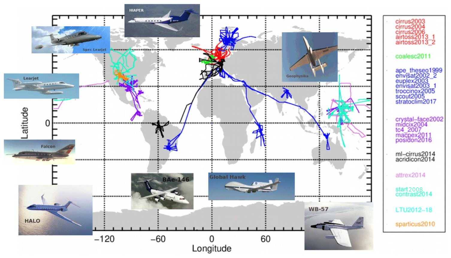
Figure 1 Aircraft flight paths during the 24 campaigns listed in Table A2. A total of 185 flights, 192 h IWC measurements, 90 h N_ice, 84 h R_ice, 116 and 331 h RH_ice in- and outside cirrus (campaign names: red – GfD Learjet, green – BAe 146, blue – Geophysica, purple – WB-57, black – HALO, light purple – Global Hawk, cyan – GV HIAPER, orange – Spec Learjet). In comparison: Schiller et al. (2008) and Krämer et al. (2009) – 52 flights, 27 h IWC measurements, 8.5 h N_ice, 8.5 h R_ice, 10 and 16 h RH_ice in- and outside cirrus.

The climatologies are advanced in several aspects in comparison to the compilations of IWC by Schiller et al. (2008), Luebke et al. (2013), and Krämer et al. (2016) and N_ice, R_ice, and RH_ice by Krämer et al. (2009).

• The number of flights and total time in cirrus increased from 104 flights for 94 h (Krämer et al., 2016) to a total of 150 flights for 168 h. The database disproportionally has extended by about a factor of 5–10 depending on the specific parameter.

• For IWC, a new data analysis method has been developed that increases the observed data volume (Appendix A2.1).

• For N_ice, observations from advanced and extended instrumentation have been added to the database; further, a new correction of the occurrence frequencies is applied (Appendix A2.2).

• The geographical spread of the observations has broadened, so that a portrayal of cirrus and humidity with respect to the midlatitude and tropical geographical regions, and also with respect to latitude and altitude, seems worthwhile.

• As in the earlier climatologies, all data underwent strict quality control.

2.2 Satellite data set

DARDAR-Nice provides observation-based estimates of N_ice obtained from CALIPSO and CloudSat measurements (Sourdeval et al., 2018a). This unique approach uses the sensitivity of lidar and radar measurements to small and large particles, respectively, to constrain two parameters of a particle size distribution (PSD) parametrization, and N_ice is subsequently estimated by direct integration of the size distribution from a minimum threshold size. For this study, we use the threshold diameter of 5 µm. DARDAR-Nice uses the parametrization by Delanoë et al. (2005), in which two normalization parameters (a slope parameter $N_{\mathrm{0}}^{\star }$ and the volume-weighted diameter D_m) are used to predict the shape of a PSD. Sourdeval et al. (2018a) have demonstrated that the method of Delanoë et al. (2005) is capable of predicting N_ice from recent in situ campaigns, by comparing its prediction based on in situ $N_{\mathrm{0}}^{\star }$ and D_m measurements to the actual in situ N_ice measurements. Good agreement was found, although it was noted that the inability of the modified gamma distribution to match the frequently bimodal shape of the measured PSDs could lead to an overestimation of N_ice in DARDAR-Nice. This problem typically occurs at temperatures above −50 ^∘C and is expected to be cloud-type dependent. Nevertheless, Sourdeval et al. (2018a) showed that the satellite N_ice remains in reasonable agreement with the in situ N_ice (within a factor of 2) from $T=-\mathrm{30}$ ^∘C down to −90 ^∘C, which should cover the entire cirrus temperature range in this study.

This evaluation of DARDAR-Nice is here repeated on the basis of five in situ campaigns archived in the Cirrus Guide II in situ database: COALESC2011, ACRIDICON2014, ATTREX2014, MLCIRRUS2014, STRATOCLIM2017. Based on the agreement between DARDAR-Nice and the in situ observations, a global N_ice climatology is derived from 10 years of satellite observations. Regional N_ice climatologies for the Arctic (90–67.7^∘ N), northern midlatitudes (67.7–23.3^∘ N), tropics (23.3^∘ N–23.3^∘ S), southern midlatitudes (23.3–67.7^∘ S), and Antarctica (67.7–90^∘ S) are analyzed in more detail. The results are presented in Sect.6.

3 Vertical distribution of cirrus and humidity from in situ observations

As an introduction, atmospheric temperature profiles in the Arctic, at midlatitudes, and in the tropics are shown in Fig. 2, (left panel, adopted from Schiller et al., 2008). Vertical profiles inside of cirrus clouds are shown for 28 flights, using blueish colors for Arctic, greenish for midlatitude, and reddish for tropical observations. It can be seen that in the tropics, with the strongest warming of the Earth's surface by the sun, the air is much warmer at upper-tropospheric altitudes than at midlatitudes or in the Arctic. The coldest atmospheric temperatures are found at the points where the slopes of the temperature profile reverses: the cold point tropopause (CPT). This is the region where the transition from the troposphere to stratosphere occurs. Above the CPT, in the stratosphere, almost no cirrus clouds are observed because it is too dry for ice formation (Smith et al., 2001; Schiller et al., 2009). The relations between temperature and altitude and the potential temperature Θ are shown in Fig. 2 middle and right panels for the different geographical regions. Θ is often used in upper-troposphere and lower-stratosphere (UT–LS) research, since it allows a clear assignment of air parcels to the associated atmospheric layer, in contrast to the temperature, whose course reverses above the CPT. The ranges of the tropical tropopause layer (TTL) and the tropical CPT are marked by magenta lines (after Fueglistaler et al., 2009).

Figure 2 Left panel: temperature vs. altitude inside of cirrus clouds (adopted from Schiller et al., 2008). Middle panel: temperature vs. potential temperature Θ. Right panel: clear-sky Θ vs. altitude. Plotted are 28 flights from the database, with blueish colors for Arctic, greenish colors for midlatitude, and reddish colors for tropical observations. Magenta lines: range of the TTL (tropical tropopause layer) and tropical CPT (cold point tropopause) (after  Fueglistaler et al., 2009).

3.1 Latitude–altitude distributions

As a first application of the Cirrus Guide II data set the distribution of cirrus clouds and humidity is shown with respect to latitude and altitude in Fig. 3. Plotted are IWC (color coded by volume mixing ratio), N_ice (color coded by concentration), R_ice (color coded by size), in-cloud and clear-sky humidity (color coded by RH_ice), and H₂O (color coded by volume mixing ratio). The color codes range from yellow to blue with increasing amount of the respective parameter; note that the data points are plotted in the order of the colors from yellow to blue. The data were collected in the latitude range from about 70^∘ north to around 20^∘ south; i.e., the northern midlatitudes and the tropics are covered by the observations. The altitude range is between about 5 and 20 km. The times of data sampling are displayed in the respective panels; a more detailed description of the database is given in Sect. 4. The way the data are presented here as individual points was chosen because the entire range of measurements is visible. Although data overlap occurs in this type of display, it is possible to identify cirrus types and microphysical processes, especially based on extreme values. As additional overview information, we have created latitude–altitude intervals (500 m altitude, 0.5^∘ latitude) and calculated the 25th, 50th (median), and 75th percentiles for all variables. These additional altitude–latitude climatologies are shown in the Supplement (Figs. S1–S3).

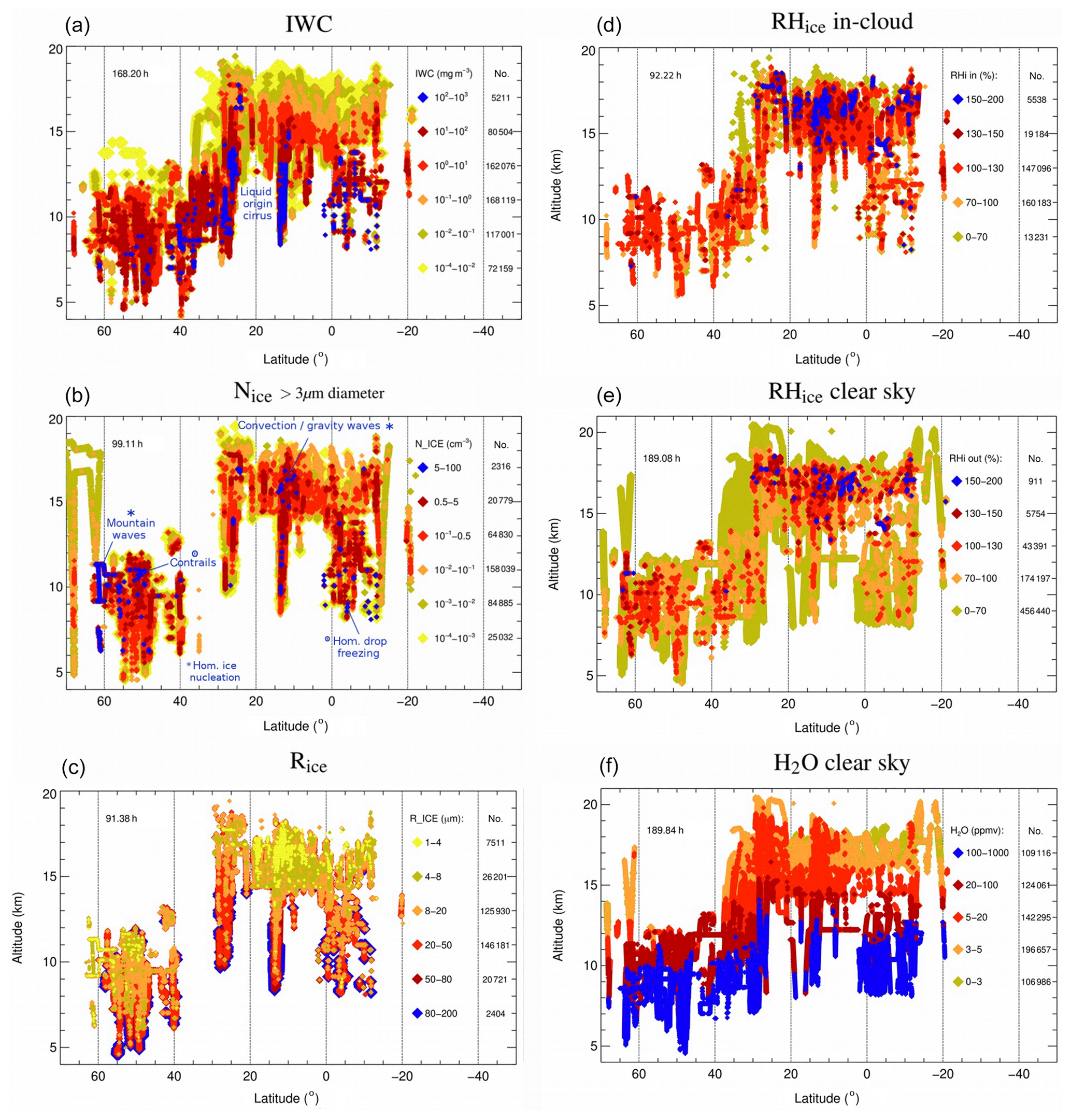
Figure 3 Cirrus cloud distribution with latitude and altitude of (left column, panels a–c) ice water content (IWC, a), ice crystal number (N_ice, size >3 µm diameter, b), and mean mass radius (R_ice, calculated from IWC∕N_ice, c). (Right column, panels d–f) In-cloud and clear-sky relative humidity with respect to ice (RH_ice, d, e) and clear-sky water vapor volume mixing ratio (H₂O, f). The field campaigns are listed in Table A1, and data evaluation methods and detection ranges of the parameters are described in Appendix A. The color codes range from yellow to blue with increasing amount of the respective parameter; for R_ice, the color code is reversed to indicate that high and low N_ice values belong to small and large R_ice; note that the data points are plotted in the order of the colors from yellow to blue; frequencies of occurrence of the parameters can be seen in Fig. 7.

Cirrus clouds are found at lower altitudes at midlatitudes and reach higher levels in the tropical region (Fig. 2). Though this structure in the measurements is influenced by the maximum or minimum height the engaged aircraft can reach, it corresponds well with the CALIPSO latitudinal height distribution of cirrus clouds, which is largely caused by the decrease in tropopause height with increasing latitude (Sassen et al., 2008).

3.1.1 in situ-origin and liquid-origin cirrus

Krämer et al. (2016), Luebke et al. (2016), and Wernli et al. (2016) describe two different cirrus types: (1) in situ-origin cirrus that form (by heterogeneous or homogeneous ice nucleation on ice-nucleating particles, INPs, or soluble solution aerosol particles) from water vapor directly as ice at T<235 K, RH_ice>100 %, and RH_w<100 % and (2) liquid-origin cirrus that evolve (also heterogeneously or homogeneously) from freezing of liquid drops in clouds at T ≳ 235 K and RH_w∼100 %.² In other words, in situ-origin cirrus are observed at the altitudes where they are formed, whereas liquid-origin cirrus are glaciated liquid clouds from further below which are lifted to the cirrus temperature region where liquid water no longer exists.

Microphysical characteristics. In the new in situ data set, containing advanced measurements and extended by several field campaigns in comparison to the earlier studies, some typical characteristics of the cirrus types and hints to ice nucleation mechanisms are visible. In the following, the cirrus types are briefly introduced using Figs. 3 and 4. The cirrus types and freezing mechanisms are summarized in Table 1.

Table 1 Typical characteristics of cirrus types in the initial stage.

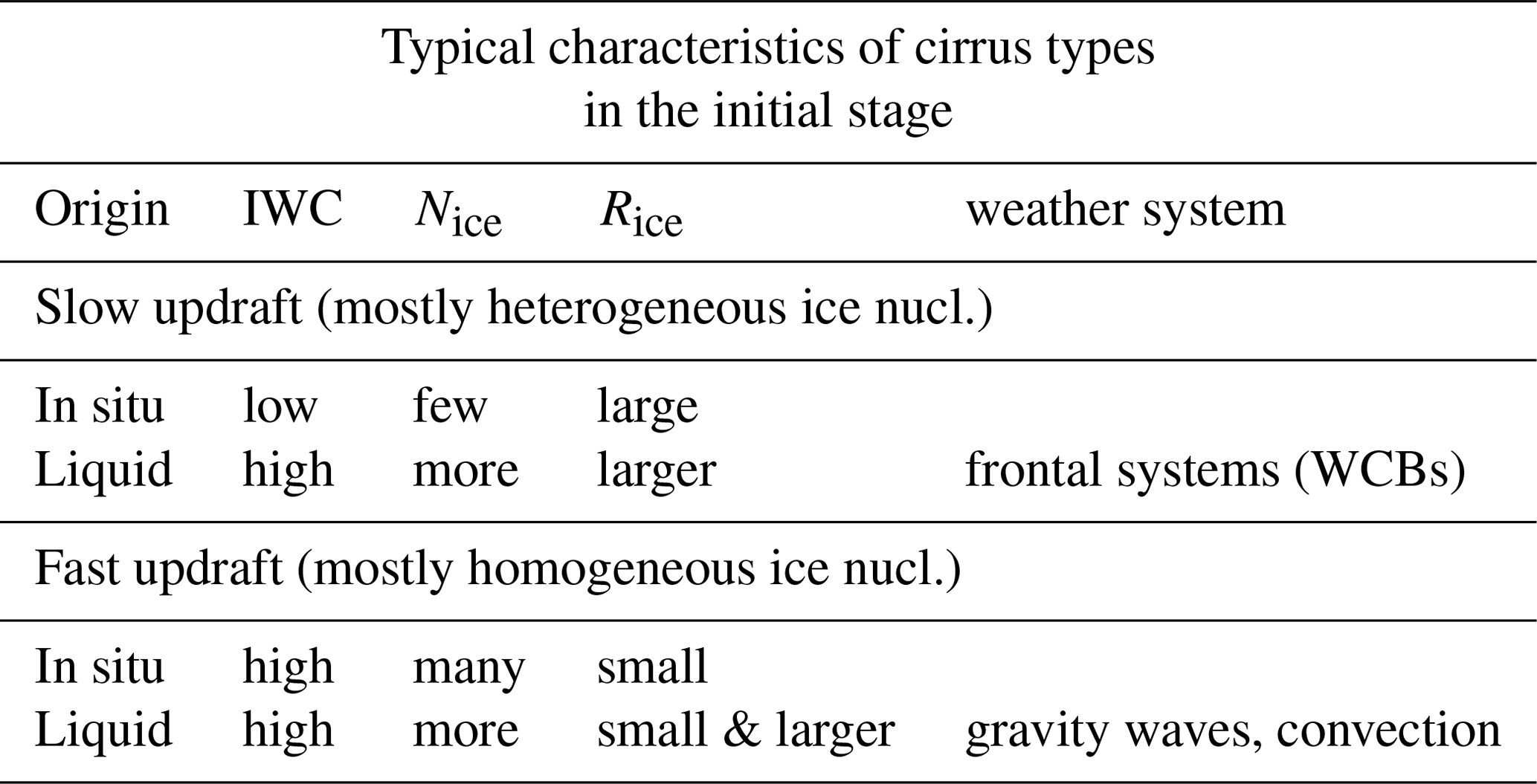
Slow updraft: ≲ 10 cm s⁻¹; fast updraft: ≳ 10 cm s⁻¹ (Kärcher and Lohmann, 2002; Krämer et al., 2016). IWC high and low: above and below the IWC median (see Fig. 7). N_ice few, more, and many: below, in between, and above the 10th and 90th N_ce percentiles (see Fig. 7).
R_ice small: ice particles ≲ 20 µm dominate the PSD, R_ice large: ice particles ≳ 20 µm dominate the PSD, max. size of several hundred micrometers in diameter, and R_ice larger: ice particles ≳ 20 µm dominate the PSD, max. size up to 1000 µm in diameter; PSD: particle size distribution.

In situ-origin cirrus can be divided in two subclasses depending on the strength of the updraft: in slow updrafts ³, in situ-origin cirrus form mostly heterogeneously (Krämer et al., 2016) and are rather optically thin with lower IWCs and few but large ice crystals. We note here that in an atmosphere free of INPs, cirrus clouds forming homogeneously may have similar characteristics to heterogeneously formed cirrus, since only a small number of ice crystals nucleate homogeneously in slow updrafts (see e.g., Spreitzer et al., 2017). Hence, in this regime, the freezing process may not be relevant for determining the cirrus properties. In fast updrafts⁴, homogeneous freezing mostly occurs regardless of the presence of INPs, since fast updrafts cause RH_ice to reach the homogeneous freezing threshold even after heterogeneous freezing. The in situ-origin cirrus that emerge in these situations are optically thicker with higher IWCs and more abundant but smaller ice crystals.

Liquid-origin cirrus stem from lower altitudes, where more water is available, so they generally consist predominantly of thicker cirrus with higher IWC, in slower updrafts together with larger ice crystals that are frozen heterogeneously at T>235 K. Small supercooled liquid cloud drops, which are much more numerous than heterogeneously formed N_ice, do not reach the cirrus cloud altitude (temperature ≲ 235 K) in the slow updrafts; the clouds completely glaciate before because of the Wegener–Bergeron–Findeisen process, where liquid drops evaporate and ice crystals grow at RH_w below and RH_ice above 100 %. In fast updrafts, liquid-origin cirrus with very many small N_ice appear. The reason is that here the supercooled liquid cloud drops can reach the altitude (temperature ∼235 K) where they freeze homogeneously (Costa et al., 2017). This is because the high updrafts keep both RH_w and RH_ice above 100 %, and thus the Wegener–Bergeron–Findeisen process does not take place (Korolev, 2007).

The meteorological situations where slow updraft in situ-origin cirrus frequently occurs (see Krämer et al., 2016) are low- and high-pressure systems (frontal and synoptic cirrus). The warm conveyor belt (WCB) of low-pressure systems can also produce slow-updraft liquid-origin cirrus. Fast-updraft in situ-origin and liquid-origin cirrus occur in gravity waves, often orographically induced, in jet streams, mesoscale convective systems, and anvils.

As outlined in the Cirrus Guide I (Krämer et al., 2016), to a certain extent cirrus types can be identified by their typical characteristics. This applies to the initial stage, after which the clouds lose the signature of the formation process, for example, by sedimentation: as long as an updraft prevails (corresponding to RH_ice>100 %), smaller ice crystals in the size range ≲ 20 µm grow to larger sizes on a timescale of tens of minutes. The larger ice crystals sediment to lower altitudes, thus removing ice surface from the cloud volume which consequently reduces the depletion of H₂O_gas (∝ RH_ice) by water vapor deposition on the ice (for more details see Spichtinger and Cziczo, 2010). The ice crystals that have fallen out of the layer deepen the cirrus extent to lower altitudes (fall streaks can extend the cirrus to several kilometers below the nucleation level; Jensen et al., 2012; Murphy, 2014), while at the same time, large ice crystals from above could sediment into the cloud volume. Altogether, the cirrus evolution is a dynamical process and the cirrus properties change in the course of a cirrus lifetime. At the final cirrus stage, i.e., when the temperature increases, the environment becomes subsaturated (RH_ice<100 %) and ice crystals sublimate, with small crystals disappearing faster than larger ones (timescales of growth and evaporation of ice crystals are shown in Kübbeler et al., 2011, their Fig. 12).

Cirrus types with the most striking features (high IWC and/or N_ice) are the easiest to identify. They could be liquid-origin or in situ-origin cirrus in fast updrafts or also liquid-origin cirrus in slow updrafts. This will be shown on the basis of Figs. 3 and 4.

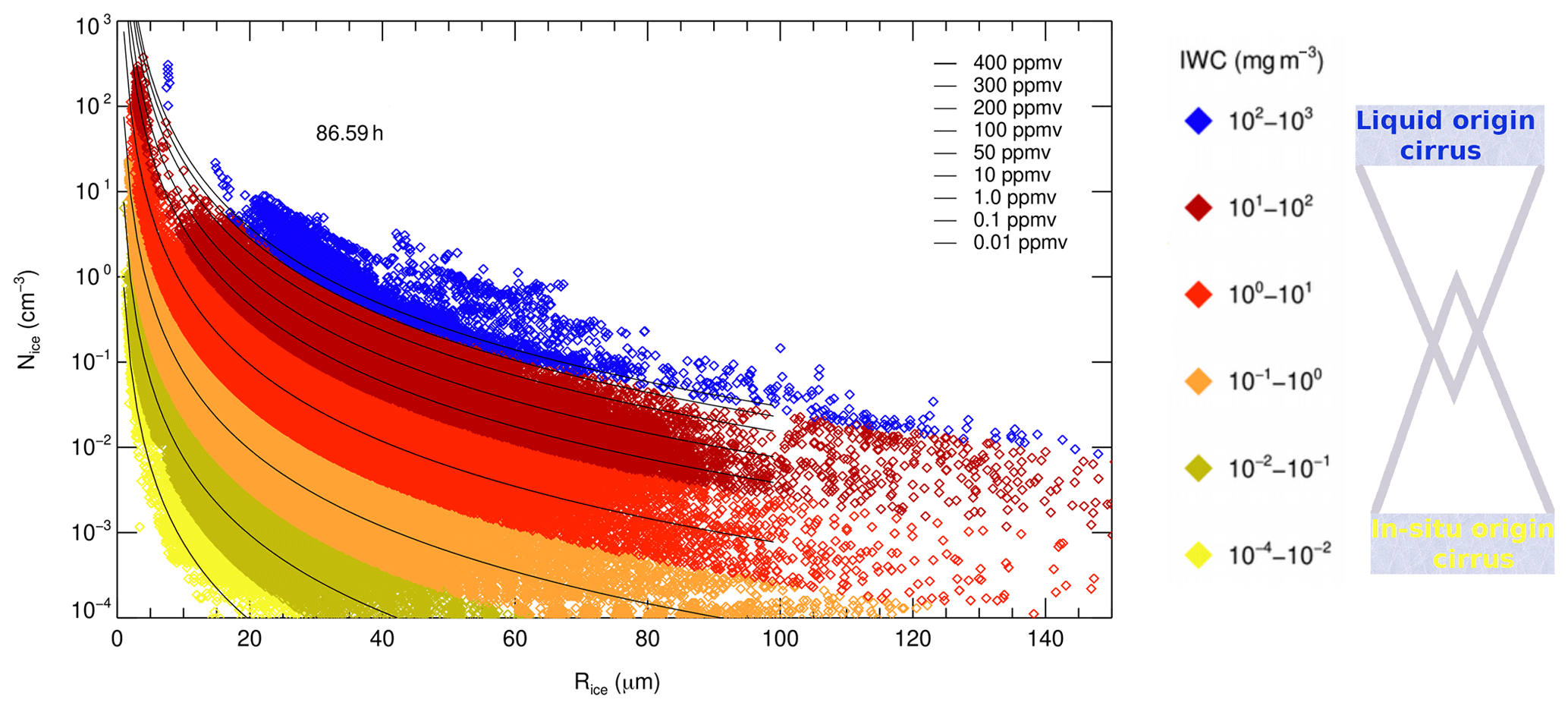
Figure 4 Relation between ice crystal concentration N_ice and mean mass radius R_ice, color coded by the ice water content IWC in milligrams per cubic meter, from ∼87 h of cirrus cloud observations (R_ice is calculated by dividing IWC by N_ice). The thin black lines are isolines of IWC as volume mixing ratio (in the order of the legend). The scheme at the right side illustrates the partitioning of the clouds between “liquid origin” and “in situ origin”: the thickest cirrus (blue points) are of liquid origin; the thinnest (yellow points) of in situ origin. As the thickness decreases, the portion of liquid-origin cirrus becomes smaller and smaller while more and more in situ-origin cirrus appear.

In Fig. 4, the relation between N_ice, R_ice, and IWC is shown for ∼87 h of cirrus cloud observations. It can be nicely seen that in the cases where N_ice is high, the ice crystals are small – because the numerous ice crystals consumed all of the available vapor, thereby suppressing further growth – while low N_ice are related to large ice crystals for a given IWC. The IWC (in milligrams per cubic meter) is indicated by the color code and results from the combination of both N_ice and R_ice. The thin black lines are isolines of IWC (plotted as volume mixing ratio, ppmv) that appear in the order shown in the legend. The symbols to the right of the figure indicate the partitioning of the clouds between liquid and in situ origin: the thickest cirrus (blue points) are of liquid origin and the thinnest (yellow points) of in situ origin. As the thickness of the cirrus decreases, the fraction contributed by liquid-origin cirrus becomes smaller and smaller while an increasing fraction is due to in situ-origin cirrus.

Most of the highest IWCs (>10 mg m⁻³, dark red and blue diamonds in Fig. 3a) are of liquid origin. They appear in the lower parts of the clouds; i.e., they are uplifted from farther below. A good example of this is the field campaign SPARTICUS in 2010, which is separately plotted in Fig. S7 of the Supplement (right panel). About 23 h of sampling in mostly liquid-origin clouds was performed over the central USA. The clouds were observed in the temperature range 210–240 K, corresponding to altitudes between 5 and 10 km; i.e., they were rather low cirrus clouds. The IWCs are mostly high (red to blue colors) and, as shown by Muhlbauer et al. (2014), ice particles of greater than a thousand micrometers in diameter were frequently encountered, indicative of liquid-origin cirrus (see Table 1). In the tropics (Fig. 3), some blue points are also detected at high altitudes of about 17 km from measurements made above the Asian monsoon in strong convective updrafts (see also Sect. 5) and consist of many ice crystals (0.1–10 cm⁻³) with medium R_ice (20–70 µm).

Generally, the IWC roughly shows a vertical structure of decreasing IWC with increasing altitude. This is caused on the one hand by the amount of available water that decreases with decreasing temperature and on the other hand because cirrus of liquid origin predominate in lower layers, whereas cirrus with in situ origin become more abundant at higher altitudes, i.e., colder temperatures. This is in accordance with the findings of Luebke et al. (2016), Wernli et al. (2016), and Wolf et al. (2018), where Luebke et al. (2016) and Wolf et al. (2018) experimentally investigated the two cloud types in midlatitudes and in the Arctic, respectively, while Wernli et al. (2016) analyzed 12 years of ERA-Interim data in the North Atlantic region (see also Sect. 6.2).

While IWC is an indication for the cirrus type, N_ice values (Fig. 3b) provide a hint to the freezing mechanism, either heterogeneous or homogeneous: high ice crystal numbers N_ice (≳ 0.5 cm⁻³, dark red and blue diamonds, Fig. 3b) are an indicator for homogeneous ice formation in fast updrafts caused by waves or convection, for both in situ-origin and liquid-origin cirrus. At midlatitudes, they are found, for example, at the tops of mountain wave clouds (the ice nucleation zone), which were observed for example behind the Norwegian mountains at around 62^∘ north. High N_ice values have also been observed in tropical deep convection around 10^∘ north, corresponding to measurements reported by Jensen et al. (2009).

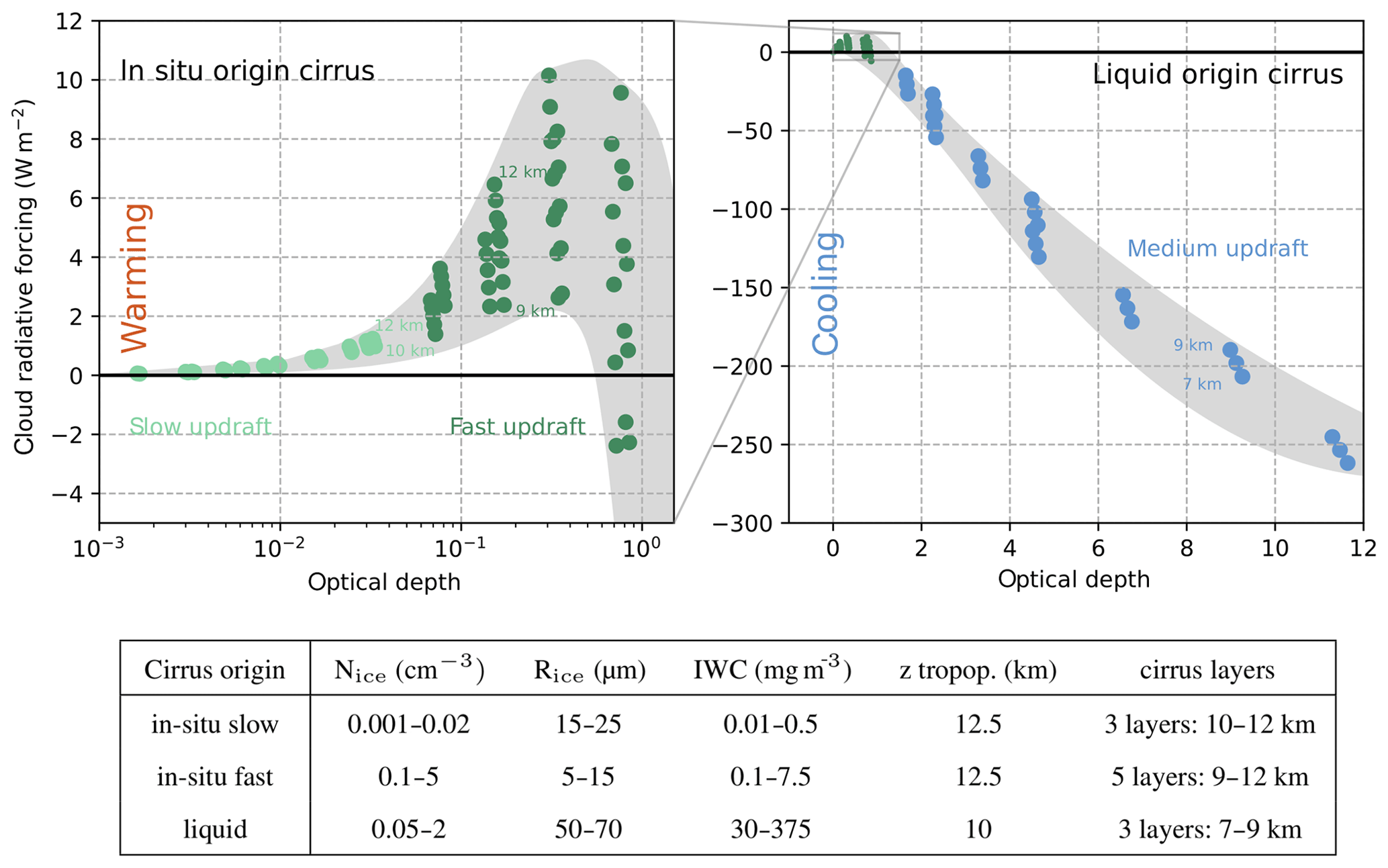
Figure 5 Simulated radiative forcing versus optical depth for exemplary in situ-origin slow- and fast-updraft cirrus (light and dark green dots) as well as liquid-origin cirrus (blue dots); the idealized scenarios are summarized in the table. Description of the idealized scenarios: a temperature profile is prescribed representative for midlatitude conditions; the surface temperature is set to 288 K (at p=1000 hPa, p exponentially decreases with height). The vertical profile of relative humidity over ice is also established, with a saturated layer of 1000 m thickness, constant subsaturation below the layer, and a strong decrease in humidity towards the stratosphere. A cirrus cloud with constant ice mass and number concentration is placed in the saturated layer. From the measurements (see Fig. 4), typical values of N_ice, R_ice and IWC are chosen for the three cirrus types (see table above). The vertical profiles are adjusted with respect to tropopause height (z tropop.) and placement of the cirrus layers in accordance with the cirrus types. For the radiative transfer calculations, the well-known two-stream radiative transfer model for ice particles by Fu and Liou (1993), with 6 bands in the solar and 12 bands in the thermal infrared regime, is used. The simulations are realized for a geographic latitude of φ=50^∘, solar surface albedo of 0.3, infrared surface emissivity of 1 and solar constant S=1340 W m⁻²; we assume equinox conditions (e.g., end of March) at local time t=12 h (for these settings, we use the modified model of Joos et al., 2014). The net cloud radiative forcing (CRF) is calculated using the fluxes at the top of atmosphere in the short wave and long wave ranges in comparison with a clear-sky case.

Another source of midlatitude high N_ice is young contrails. Note however, that these high N_ice values exist only for a short time. This is because high ice crystal numbers are associated with small ice crystal sizes (yellow diamonds in the bottom left panel; see also Fig. 4) that grow and/or evaporate quickly. At lower altitudes, N_ice tends to be lower and the crystals are larger, because large crystals having lower concentrations sediment out from the cloud tops, and, as mentioned above, liquid-origin cirrus with characteristic large ice crystals are also common in this altitude range. In the tropics, high N_ice values at high altitudes are induced by in situ homogeneous freezing in convection or gravity waves (see also Jensen et al., 2013a). At cloud bases, such high N_ice values are most probably of liquid origin, initiated by homogeneous freezing of supercooled drops.

A more detailed discussion of the microphysical properties of cirrus including frequencies of occurrence of specific signatures which cannot be seen from Fig. 3 is given in Sect. 4.

Radiative characteristics. A motivation to study cirrus clouds is to investigate the radiative properties on the basis of the findings on their microphysical properties. In the Cirrus Guide I, Krämer et al. (2016) speculated that the physically and optically thinner in situ, slow-updraft cirrus cause a warming effect, while thicker fast-updraft in situ-origin and, particularly, thick liquid-origin cirrus have the potential to cool. Here, we show a first estimate of the radiative forcing of typical in situ-origin slow- and fast-updraft as well as liquid-origin cirrus (Fig. 5). To this end, radiative transfer calculations for idealized scenarios under specific conditions are conducted, with solar zenith angles corresponding to noon at the equinox, which are briefly described in the caption of Fig. 5.

In the left panel of Fig. 5, the radiative forcing of the slow (light green) and fast (dark green) in situ-origin cirrus is displayed with respect to optical depth. This panel is expanded from the right panel, where the forcing of the liquid-origin cirrus is shown. Obviously, the net radiative forcing of the in situ-origin cirrus is much smaller than that of liquid origin and, moreover, changes the sign from warming to cooling.

In more detail, the slow in situ-origin cirrus have only small optical depth (τ) between 0.001 and 0.05, resulting in a slight net warming effect of not larger than about 1.5 W m⁻². The optical depth of fast in situ-origin cirrus is larger (τ: 0.05–1), but most of them are also warming (2–10 W m⁻²). The thickest fast-updraft in situ-origin cirrus at the lowest altitudes change the sign of their net forcing; i.e., they switch to a slight cooling effect. The reason for the sign change is the warmer temperature at lower altitude that reduces the warming effect of the longwave infrared radiation. The results of the radiative forcing calculations for the slow- and fast-updraft cirrus are in agreement with investigations from lidar observations reported by Kienast-Sjögren et al. (2016) and Campbell et al. (2016), who observed cirrus with optical depth up to 1 and 3, respectively, and found a decreasing warming effect with decreasing optical depth. Campbell et al. (2016) even reported a slight cooling effect at the warmest observed cirrus. The liquid-origin cirrus, however, mostly found in the warmest cirrus layers, have large optical depths (τ: 1–12), which is larger than the range of cirrus optical depth reported in many studies (the maximum optical depth is often found to be 1–3, e.g., Sassen et al., 2008; Kienast-Sjögren et al., 2016; Campbell et al., 2016; Mitchell et al., 2018; note that this is likely because the lidar technique, often used to investigate cirrus cloud optical properties, has restrictions in the τ determination of thicker ice clouds). A consequence of the large optical thickness is a quite strong net cooling effect (−15 to −250 W m⁻²) of liquid-origin cirrus. These values are of the same order of magnitude as reported from direct measurements inside of cirrus clouds (Wendisch et al., 2007; Joos, 2019).

Thus, from these first very idealized simulations, we can conclude that in situ-formed cirrus clouds are most likely to warm the atmosphere, whereas liquid-origin ice clouds have the potential for strong cooling. Note here that we only investigate local time 12 h, where the cooling is probably most pronounced. For lower sun position (i.e., larger zenith angle) the cooling is probably reduced, and during nighttime cirrus clouds can only warm the atmosphere (due to the thermal greenhouse effect). Thus, the net effect of cirrus clouds averaged over the whole daily cycle is not yet clear. Such investigations go beyond the scope of this study and are the subject of future work.

3.1.2 Humidity

The distribution of in-cloud and clear-sky RH_ice as well as water vapor H₂O with latitude and altitude is shown in Fig. 3 (right column, panels d–f). It can nicely be seen how the amount of H₂O decreases with altitude (panel f). The clear-sky RH_ice (panel e) ranges from very dry conditions (<70 % green and orange diamonds) up to highly supersaturated regions (>130 %, dark red and blue diamonds), which mainly are found at high altitudes in the tropics. Such high supersaturations are also occasionally found inside of the tropical cirrus clouds (panel d). The behavior of RH_ice will be further discussed in Sects. 4 and 5.

4 In situ climatologies

With the term climatologies we refer here to statistical evaluations of the available variables with regard to temperature or potential temperature.

4.1 The IWC–T parameter space: median N_ice, R_ice, and RH_ice

In the Cirrus Guide I (Krämer et al., 2016), observations and model simulations are portrayed in the ice water content–temperature (IWC–T) parameter space. One result of the simulations is that IWC and N_ice are correlated with each other. This relationship has been confirmed for some meteorological situations by examples from six individual field campaigns. The database of combined IWC–N_ice measurements has grown considerably since then and with it the covered temperature range of the observations. In the Cirrus Guide I, only a few observations below 200 K were available.

With the extended Cirrus Guide II data set, we further investigate the statistics of N_ice but also the corresponding mean mass size R_ice and the in-cloud RH_ice in the IWC–T parameter space. In Fig. 6, medians of the respective parameters are presented in intervals (five IWC intervals per order of magnitude, 1 K temperature intervals) covering the entire IWC–T parameter space. The variability of the parameters can be seen in Figs. S1–S3 of the Supplement, where the 25th, 50th (median), and 75th percentiles for the variables are shown.

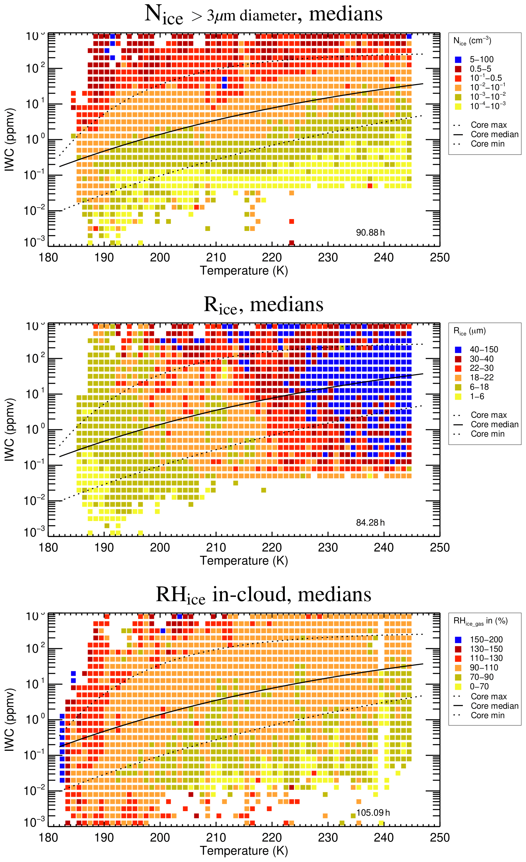
Figure 6 Median N_ice, R_ice, and RH_ice in intervals in the IWC–T parameter space (five IWC intervals per order of magnitude, 1 K temperature intervals). The color codes of N_ice and RH_ice range from yellow to blue with increasing amount of the respective parameter; for R_ice, the color code is reversed to indicate that high and low N_ice values belong to small and large R_ice. Black solid and dotted lines: median, min, and max IWC of the core IWC band of Schiller et al. (2008). The variability of the parameters (25th, 50th (median), and 75th percentiles) is shown in Figs. S1–S3 of the Supplement.

4.1.1 IWC–T–N_ice and R_ice relation

Observational evidence for the correlation between IWC and N_ice can be nicely seen in the upper panel of Fig. 6. Almost symmetrical colored bands of N_ice can be seen across the entire IWC–T parameter space (N_ice concentration increases from yellow to blue). With decreasing temperature, the same N_ice numbers cause lower IWC values, which is caused by the likewise decreasing available water content of the air. This finding might be of importance for parametrizations used in global models or satellite retrieval algorithms, where IWC is often the only available parameter that characterizes cirrus clouds, but functions are used to assign N_ice to specific IWCs. This new analysis can be used (after some smoothing of the bands, which will be the subject of a follow-up study) as a lookup table to derive N_ice from the information of temperature and IWC.

The ice crystal sizes also form colored bands in the IWC–T parameter space (Fig. 6, middle panel; R_ice increases from yellow to blue, running diagonally through the IWC–T room with the size of the ice crystals increasing with increasing temperature (and thus decreasing amount of available water). This is because R_ice is calculated from the third root of the IWC divided by N_ice, as described in Sect. 1. However, the R_ice bands are somewhat less clearly delineated from each other than the N_ice bands. They might be smoothed in the follow-up study, so that R_ice can also be assigned to the IWC–T data points.

One could have expected to find distinct patterns for in situ-origin and liquid-origin cirrus in this type of analysis to quantify the characteristics of the cirrus types shown in Table 1. However, the differences are merged by the calculation of median values in the overlap regions of the types in the IWC–T parameter space. Nevertheless, we believe that the more heterogeneous structure of the R_ice bands is caused by the different cirrus types, because the ice crystal size is their most pronounced difference. A longer-term research goal is to derive the IWC–T–N_ice–R_ice relations separately for in situ-origin and liquid-origin cirrus.

4.1.2 IWC–T–RH_ice relation

In the bottom panel of Fig. 6, median in-cloud RH_ice values are shown in the IWC–T parameter space. For RH_ice patterns are also visible: RH_ice decreases with decreasing IWC. Above the median IWC (black solid line), RH_ice is mostly between 90 % and 110 % (orange data points), i.e., around saturation. This corresponds to the existence phase of the cirrus (between 110 %–100 % and 100 %–90 %, the ice crystals slowly grow and/or evaporate). Below the median IWC, the median RH_ice values decrease with decreasing IWC (green and yellow data points), reflecting the evaporation phase of the cirrus clouds. Interesting is the distribution of the higher supersaturations (red and blue points): at low temperatures, the clouds tend to higher supersaturations. This has been discussed by Krämer et al. (2009) for thin cirrus (low IWC) and explained by the corresponding low N_ice, whose small ice surface cannot efficiently deplete the water vapor. However, the supersaturations are also seen at high IWC (∼ high N_ice). The reason for that is the vertical velocity, which is – together with the ice surface and temperature – a driver of the RH_ice (RH${}_{\mathrm{ice}}={\mathrm{H}}_{\mathrm{2}}\mathrm{O}/{\mathrm{H}}_{\mathrm{2}}{\mathrm{O}}_{\mathrm{sat},\mathrm{ice}}\left(T\right)$). The air inside of clouds is supersaturated in cases in which the depletion of H₂O on the available ice surface (decrease in RH_ice) cannot compensate for the increase in RH_ice caused by the cooling of the air (decrease in H₂O_sat,ice(T) with decreasing temperature). High IWC, always coinciding with high N_ice, appears in high updrafts, in in situ-origin as well as in liquid-origin cirrus. These high updrafts allow that the supersaturations remain high despite the large ice surfaces available for deposition of excess water vapor. This was also reported by Petzold et al. (2017), who observed high RH_ice together with high N_ice in tropical convective cirrus onboard passenger aircraft (IAGOS).

4.2 Entire in situ climatologies

The Cirrus Guide II data set shown in Fig. 3 is now displayed as frequencies of occurrence as a function of temperature (binned in 1 K intervals, Fig. 7) and discussed in comparison to the earlier in situ climatologies presented by Schiller et al. (2008), Krämer et al. (2009), and Luebke et al. (2013) (Fig. S6, Supplement). Further, as mentioned above, the new data set is large enough to split it in midlatitude and tropical cirrus. The differing cirrus cloud properties are presented in Fig. 8 and the respective clear-sky and in-cloud RH_ice in Fig. 9.

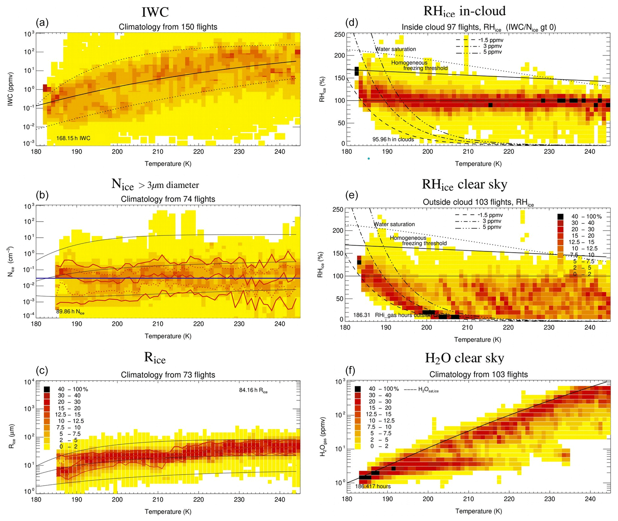
Figure 7 Frequencies of occurrence in dependence on temperature, binned in 1 K intervals of ice water content (IWC; a; black solid and dotted lines: median, min, and max IWC of the core IWC band of Schiller et al., 2008). Ice crystal number (N_ice, size >3 µm diameter, b; red lines: 10th, 25th, 50th, 75th, and 90th N_ice percentiles; blue line: fit through median N_ice values (median N_ice: 0.03 cm⁻³; 10th, 25th, 75th, and 90th percentiles: 0.002, 0.007, 0.102, 0.3 cm⁻³); black lines: minimum, middle, and maximum N_ice of Krämer et al., 2009). Mass mean radius (R_ice: calculated from IWC and N_ice, c; red lines: 10th, 25th, 50th, 75th, 90th R_ice percentiles; black lines: minimum, middle, and maximum R_ice of Krämer et al., 2009). In-cloud and clear-sky relative humidity with respect to ice (RH_ice, d, e), and water vapor volume mixing ratio (H₂O, f). The field campaigns included in the data analysis are listed in Table A2. Data evaluation methods and detection ranges of the parameters are described in Appendix A. Note that for N_ice – and thus R_ice – the hours spent in clouds is less than in Fig. 3. The reason is that for the calculation of data frequency distributions only measurements covering the same detection range are used (see also Appendix A2).

4.2.1 Ice water content (IWC–T)

Figure 7a depicts the IWC. The black solid and dotted lines represent the median, minimum, and maximum IWC of the core IWC band, that is the envelope of the most frequent IWC (>5 % per IWC–T bin; Schiller et al., 2008).

The number of hours spent sampling in cirrus clouds increased from 27 h in Schiller et al. (2008), 38 h in Luebke et al. (2013), and 94 h in (Krämer et al., 2016) to 168 h in the new extended data set. Part of the additional data are due to the new IWC data product that is applied to all campaigns and combines the IWC from total water measurements and the IWC derived from cloud particle size distributions (see Appendix A2.1).

However, the median IWC and the core IWC band – decreasing with temperature as described by Schiller et al. (2008) – is still valid, showing that the IWC measurement techniques are robust and that the IWC is a stable parameter describing cirrus clouds. Note here that at temperatures ≲ 200 K data points underneath the lower dotted line are not unambiguously identified as clouds, while above about 200 K this threshold is 0.05 ppmv. For more detail see also Appendix A2.1.

4.2.2 Ice crystal number (N_ice–T)

About 90 h of N_ice observations are shown in Fig. 7b⁵, which is an increase of about a factor of 10 in comparison to the data set of Krämer et al. (2009), who compiled 8.5 h (Fig. S6, Supplement). For N_ice, the picture has greatly changed when comparing the old and the new data sets. This change is on the one hand due to an extension of the lower detection limit of N_ice from $\mathrm{4}\times {\mathrm{10}}^{-\mathrm{3}}$ to 10⁻⁴ cm⁻³ (see Appendix A2.2), but also because the new data set represents a better mixture of different meteorological situations. For example, the higher N_ice values at warmer temperatures in the Krämer et al. (2009) data set (Fig. S6, Supplement) were caused by flights where lee wave cirrus behind the Norwegian mountains were probed (see also Fig. 3, blue diamonds at around 60^∘ north). Also, at temperatures colder than about 200 K, N_ice was most often very low. Further, the enhanced occurrence frequencies at the lowest concentrations seen in the earlier data set are corrected in the new data evaluation procedures (Figs. A2 and  S6, Supplement, middle left panel).

A total of 90 h of aircraft N_ice observations within cirrus clouds is a tremendous amount when taking into account the necessary effort. However, this is still far from being representative for the distribution of N_ice in the atmosphere. We nevertheless calculated 10th, 25th, 50th, 75th, and 90th percentiles, which are shown as thin, dotted, and solid lines in Fig. 7b. Note that the 10th and 90th percentiles enclose the core region of N_ice, i.e., the envelope of the most frequent N_ice (>5 % per N_ice–T bin). Fits through these percentiles and the median N_ice reveal no temperature dependence of N_ice (10 %, median, and 90 % N_ice: 0.002, 0.03, and 0.3 cm⁻³). This is different to the slight decrease with temperature of the minimum, middle, and maximum N_ice lines shown by Krämer et al. (2009), which was, as discussed above, caused by two flights with high N_ice at comparatively warm temperatures.

It is an open question why the N_ice values do not increase with decreasing temperature, as would be expected from theoretical homogeneous freezing calculations (see e.g., Kärcher and Lohmann, 2002). This has been investigated by Gryspeerdt et al. (2018) based on a 10-year global data set retrieved from satellite observations (DARDAR-N_ice; Sourdeval et al., 2018a; see also Sect. 6). Gryspeerdt et al. (2018) analyzed the N_ice (>5 µm) only at cloud tops and also those throughout the cirrus clouds. From the cloud top analysis, a clear increase in N_ice with decreasing temperature was obvious; while integrating throughout the cirrus this temperature dependence becomes much weaker, though it is still present. Gryspeerdt et al. (2018) propose that the missing temperature dependence in the in situ results could be due to a lack of in situ measurements near the cloud top, where the temperature dependence is strongest. Another reason could be that the higher N_ice values are short-lived (see Sect. 3.1.1) and thus not easy to trace by aircraft.

A further consideration of N_ice frequencies of occurrence on global and regional scales derived from satellite remote sensing will be presented in Sect. 6.

4.2.3 Ice crystal mean mass radius (R_ice–T)

The ice crystal mean size is calculated as mean mass radius R_ice as shown in Footnote 2. R_ice is close to the common effective cloud particle radius R_eff (∼ ice volume divided by area) but can be calculated without knowing details of the ice particle size distribution (see also Krämer et al., 2016).

A total of 84 h of observations are compiled in Fig. 7c. Overall, the mean mass R_ice ranges from about 1 to 100 µm, while individual ice crystals in cirrus can reach sizes up to 1000 µm or even larger. The R_ice core band (frequencies ≳ 5 % per R_ice–T bin) decreases slightly as the temperature decreases, which is caused by the decrease in the IWC core band, since the N_ice band is not dependent on temperature (see previous section).

The 10th, 25th, 50th, 75th, and 90th percentiles of the data set are plotted as thin, dotted, and solid red lines. The black lines represent the minimum, middle, and maximum R_ice shown by Krämer et al. (2009) (see Fig. S6, Supplement). The range of R_ice has shifted slightly to larger sizes in the new data set, which is caused by the N_ice range extended towards lower concentrations that mainly consist of larger ice crystals.

Remarkable is the drop of the most frequent R_ice from larger to smaller ice crystals seen at around 215 K. This is probably the approximate temperature up to which liquid-origin clouds are detected (see Luebke et al., 2016; Sourdeval et al., 2018a, and also Sect. 6.2), which are characterized by larger ice crystals than in situ-origin cirrus (Krämer et al., 2016). At higher temperatures where both liquid and in situ-origin cirrus prevail, higher IWCs – and thus also a larger R_ice – occur more often than at lower temperature, where only the thinner in situ-origin clouds exist. This is especially true at midlatitudes. In the tropics the liquid-origin cirrus also reach lower temperatures and thus no sudden drop of R_ice is observed (see Fig. 8c, f). The bifurcated structure of the most frequent R_ice which can be seen for temperatures ≲ 190 K is discussed in Sect. 4.3.1 (vii).

Figure 8 Same as Fig. 7a–c, but for midlatitudes and tropics (WCBs: warm conveyor belts; MCS: mesoscale convective systems; TTL: tropical tropopause layer). The field campaigns are listed in Table A2.

4.2.4 Clear-sky and in-cloud RH_ice (RH_ice–T)

The new RH_ice clear-sky and in-cloud data sets are displayed in Fig. 7e, d. The respective earlier data sets of Krämer et al. (2009) are shown in Fig. S6, Supplement. The overall picture of the RH_ice distributions has not changed substantially, though the amount of in-cloud data in the database has increased from 10 h of measurements to about 96 h, and the clear-sky observation time has increased from 16 to 186 h. The only small difference is found in the in-cloud RH_ice, potentially caused by the larger amount of data: below about 200 K, where high supersaturations (>120 %) occur more often and low subsaturations (<80 %) less often. At higher temperatures, the peak of RH_ice frequencies at 100 % is more pronounced.

For the new data set, in addition to the clear-sky RH_ice the absolute water vapor volume mixing ratio H₂O in Fig. 7f is plotted. To guide the eye, water vapor saturation with respect to ice, H₂O_sat,ice, is drawn as a black solid line. The decrease in H₂O with temperature is nicely seen in this panel, and clear-sky supersaturations appear in this portrayal as data points above H₂O_sat,ice.

4.3 Midlatitudes and tropics

4.3.1 Midlatitude and tropical cirrus clouds

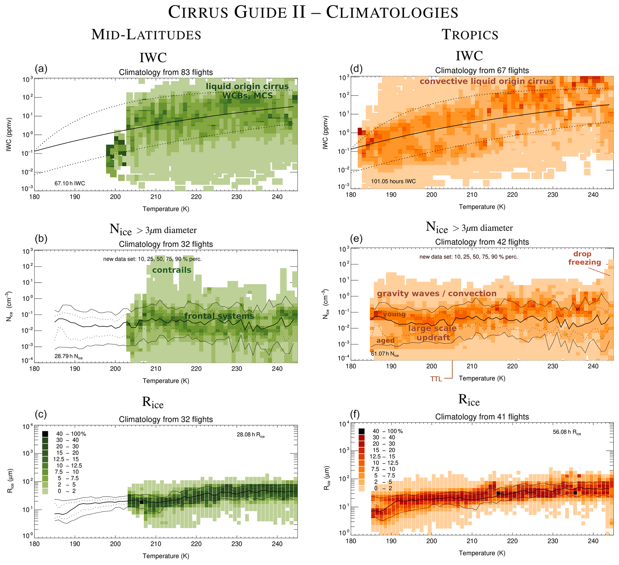
The data sets of midlatitude and tropical cirrus consist of 67 and 101 h of IWC, 29 and 61 h of N_ice, and 28 and 56 h of R_ice measurements, respectively. This section describes some of the pronounced characteristics of midlatitudes and tropical cirrus, which are displayed in Fig. 8 (greenish and reddish colors represent midlatitude and tropical cirrus).

• Temperature ranges. Comparing midlatitude and tropical cirrus, the first obvious difference – as expected when looking at the temperature profiles in Fig. 2 – is the temperature range. The observed midlatitude cirrus rarely occur below 200 K, while tropical cirrus are detected down to temperatures of 182 K. The core IWC, N_ice, and R_ice ranges of both midlatitude and tropical cirrus correspond to the total climatology (see Fig. 7).

• ii.

  Midlatitude WCBs and MCS. At European midlatitudes, the most frequent cirrus can be assigned to slow updrafts in frontal systems (WCBs: warm conveyor belts) containing both liquid-origin and in situ-origin cirrus. High IWCs stem mostly from liquid-origin WCB cirrus. Above the central USA, small and mesoscale convective systems (MCSs) with faster updrafts are more frequent. The resulting liquid-origin cirrus are thicker than the European cirrus; i.e., the ice crystals are larger and the IWC is higher (see also Krämer et al., 2016).

• iii.

  Contrails. A striking feature in the cirrus observations is N_ice values of up to several hundreds per cubic centimeter, which are found at midlatitudes in the temperature range of about 210–220 K, which corresponds to about 10 km altitude (see Fig. 2), the typical cruising level of passenger aircraft. They can be attributed to young contrails, which were a topic of investigation during COALESC 2011 (Jones et al., 2012) and also ML-CIRRUS 2014 (Voigt et al., 2017). Higher midlatitude N_ice at higher temperatures are most probably in situ-origin cirrus caused by stronger updrafts in, for example, mountain waves.

• iv.

  Drop freezing. High N_ice values between 10 and 100 cm⁻3 or even more are found above 235 K. Such high concentrations together with small R_ice values are typical for supercooled liquid cloud drops that might be frozen by spontaneous homogeneous drop freezing (which occurs at the latest at around 235 K in the atmosphere). In any case, these cloud particles are an indication for liquid-origin clouds caused by tropical or midlatitude convective systems with fast updrafts.

• v.

  Tropical convection. In contrast, in tropical cirrus, and particularly for temperatures ≳ 220 K, high IWCs and N_ice above the core range – corresponding to convective liquid-origin cirrus – become more frequent, while R_ice tends to be smaller. This is most likely caused by the fast convective vertical velocities that often let clouds in the mixed-phase temperature regime rise to the cirrus altitude range.

• vi.

  Tropical deep convection. Also remarkable is that in the tropics, massive convective liquid-origin cirrus carrying a high IWC – often accompanied by high N_ice – are detected down to very cold temperatures (<200 K), which corresponds to high altitudes up to 17 km. The thickest cirrus with very high IWC and N_ice can also be seen in Fig. 3a, b (distribution of cirrus with latitude; blue data points represent liquid-origin cirrus with a high IWC and N_ice) at around 25^∘ northern latitude and 16–18 km altitude. These exceptional thick and cold cirrus at high altitudes were observed in the Asian monsoon tropical tropopause layer (TTL). The numerous observed small ice crystals are most likely generated by in situ homogeneous ice nucleation, triggered either by fast updrafts in gravity waves (see also Spichtinger and Krämer, 2013; Jensen et al., 2013a) or by deep convection. They often occur in the tops of massive liquid-origin cirrus with very high IWC; a theoretical description of such clouds is given by Jensen and Ackerman (2006).

• vii.

  TTL cirrus. The discussion of cirrus clouds in the tropical tropopause layer is presented in Sect. 5.

Figure 9 Same as Fig. 7d–f, but for midlatitudes and tropics. The field campaigns are listed in Table A2.

4.3.2 Midlatitude and tropical humidity

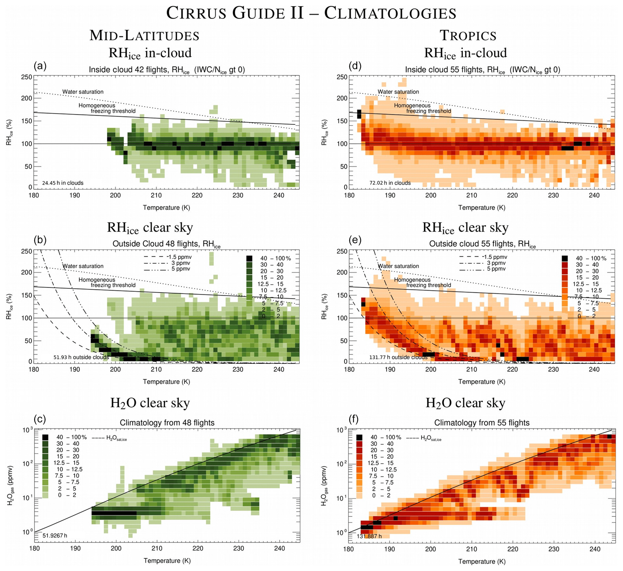
The midlatitude and tropical humidity data sets include 24 and 72 h of in-cloud RH_ice and 51 and 132 h of clear-sky RH_ice and H₂O measurements, which are displayed in Fig. 9 with the same color code as in Fig. 8.

In clear sky at temperatures higher than about 200 K, RH_ice is most often below saturation and randomly distributed in both midlatitudes and tropics (Fig. 9b, e). Clear-sky supersaturations occurs less frequently, simply because they only take place in those periods when moist air parcels are cooled towards the ice nucleation thresholds (heterogeneous or homogeneous), which are rare compared to drier conditions of the atmosphere.

Below about 200 K, i.e., in the TTL (see also Sect. 5), the clear-sky RH_ice distribution looks very different. In this region, H₂O is low and its variability is only small (Fig. 9c, f). We plotted lines of constant H₂O (1.5, 3, and 5 ppmv) in the clear-sky RH_ice panels to illustrate that for constant H₂O, RH_ice increases only due to the decrease in temperature, i.e., H₂O_sat,ice. Thus it can be seen that at midlatitudes RH_ice values mostly represent H₂O values around 3 ppmv and in the tropics between 1.5 and 3 ppmv. Since in the tropics much colder temperatures are reached, the respective RH_ice ranges from 10 up to about 150 % or even more (see also Jensen et al., 2017b; Krämer et al., 2009, who already presented parts of the data shown here).

Clear-sky RH_ice values above the homogeneous freezing line are under discussion, because they would indicate that no supercooled liquid aerosol particles are present to initiate freezing or that the homogeneous freezing is prevented, for example by organic material contained in the aerosol particles. More probably, these few data points are outliers; note also that the uncertainty of RH_ice rises from approximately 10 % at warmer temperatures to about 20 % at colder temperatures (Krämer et al., 2009).

Inside of cirrus, the peak of the RH_ice frequency distribution is mostly around the thermodynamical equilibrium value of 100 % (saturation) at midlatitudes as well as in the tropics (Fig. 9a, d; see also Jensen et al., 2017b; Krämer et al., 2009). However, in the TTL, at the coldest prevailing temperatures (≲ 190 K), supersaturation increasingly becomes the most common condition, which is discussed in more detail in Sect. 5. High supersaturations at low temperatures were also reported by Krämer et al. (2009) and Jensen et al. (2013a), and the reason given for the existence of such high supersaturation is low N_ice concentrations, which were mostly present at low temperatures in these observations (Fig. S6, Supplement). However, Jensen et al. (2013a) also showed that RH_ice rapidly drops to saturation in the presence of many ice crystals. As can be seen from Fig. 8e (and discussed in Sect. 4.2.2), in the new data set N_ice values cover a broader concentration range in comparison to the earlier data (Fig. S6, Supplement), while RH_ice is supersaturated in most cases. This is not straightforward to understand due to the complex relation between RH_ice and N_ice. We will investigate the TTL supersaturations in cirrus clouds in a follow-up study.

5 TTL in situ climatologies in- and outside of the Asian monsoon anticyclone

The tropical tropopause layer is the region above the upper level of main convective outflow, where the transition from the troposphere to stratosphere occurs. It is placed at temperatures <205 K between ∼150 hPa, 355 K potential temperature and 14 km, and 70 hPa, 425 K and 18.5 km (Fueglistaler et al., 2009; see also Fig. 2). The coldest temperatures are found here at the point where the slope of the temperature profile reverses (cold point tropopause, CPT). In the TTL, the prevailing dynamical conditions are very slow large-scale updrafts superimposed by a spectrum of high-frequency gravity waves (i.e., Spichtinger and Krämer, 2013; Dinh et al., 2016; Jensen et al., 2017a; Podglajen et al., 2017). In addition, deep convection with fast updrafts occasionally overshoots into the TTL.

Cirrus clouds and humidity in the TTL deserve a special consideration, because this region represents the main pathway by which water vapor enters the upper troposphere and lower stratosphere (UT–LS) where it is further distributed over long distances (e.g., Brewer, 1949; Holton et al., 1995; Rolf et al., 2018; Vogel et al., 2016; Ploeger et al., 2013). This is of importance, because water vapor is a greenhouse gas that has a significant impact on the climate, with the greatest sensitivity in the tropical UT–LS (Solomon et al., 2010; Riese et al., 2012), but also in the LS at high latitudes where it is being transported from the tropics. Cirrus clouds are of particular relevance as regulators of the partitioning of H₂O between gas and ice phases. Furthermore, they have a climate feedback themselves by influencing the Earth's radiation balance (e.g., Boucher et al., 2013). Thus, the simultaneous observation and analysis of both cirrus clouds and humidity (H₂O) in this climatically crucial region are of special interest.

This section specifically reports cirrus clouds together with humidity (from the climatologies presented in Sect. 4), which was recently observed for the first time in the TTL in the Asian monsoon anticyclone (June to September) in comparison to observations in the surrounding tropical regions. As the Asian monsoon is characterized by strong convective activity, this comparison will show the difference to less active, calmer areas (note here that the ATTREX and POSIDON campaigns were in western Pacific highly convective regions; however, the flights from these campaigns generally did not sample fresh convective outflow). Observations of Asian monsoon TTL cirrus clouds and humidity are of particular importance because, amongst other trace species, large amounts of H₂O and also cloud particles are convectively transported upwards from far below, where the additional H₂O in turn often causes cirrus formation (e.g., Ueyama et al., 2018, and references therein). Directly injected H₂O or H₂O from sublimated ice crystals can then be mixed up into the stratosphere. Thus, the Asian monsoon anticyclone represents a significant gateway for H₂O between UT and LS (e.g., Fueglistaler et al., 2009; Ploeger et al., 2013), and currently it is under discussion to what extent cirrus cloud particles contribute to the amount of H₂O entering the stratosphere (e.g., Ueyama et al., 2018, and references therein).

The airborne measurements in the Asian monsoon (see Fig. 1 and Tables A1 and A2) were performed during July–August 2017 out of Kathmandu, Nepal, during a field campaign as part of the StratoClim project (http://www.stratoclim.org/, last access: 15 January 2020). An overview of the observations is given in Figs. 10, 11, and 12, where the frequencies of IWC, N_ice, R_ice, and in-cloud, clear-sky RH_ice as well as the clear-sky H₂O volume mixing ratio are shown in the temperature and also the potential temperature Θ parameter space.⁶

Most of the measurements during StratoClim are performed at temperatures ≲ 205 K, corresponding to potential temperatures ≳ 355 K and altitudes ≳ 14 km, i.e., in the TTL (marked in the middle panels of the figures).

The surrounding, typically calmer tropical TTL regions are represented by observations during the campaigns shown in Fig. 1 and listed in Tables A1 and A2. The majority of the data were sampled during ATTREX_2014 and POSIDON_2016. The TTL measurements in the temperature parameter space are shown in Figs. 8 and 9; in these plots, the Asian monsoon observations are included, but since the measurements represent only a small part of all TTL observations, excluding the StratoClim campaign only slightly changes the frequency distributions. Thus, the figures are representative for the TTL outside of the Asian monsoon anticyclone, and we refrain from showing an additional figure. The measurements in the Θ parameter space (StratoClim excluded) are presented in Figs. 11, left column, and 12, left column.

5.1 TTL cirrus clouds

5.1.1 Temperature parameter space

In the tropics outside of the Asian monsoon (Fig. 8, right column, panels d–f)), cirrus IWC and N_ice range from very low to quite high values. We want to draw attention to a special feature of the most frequently occurring cirrus N_ice (panel e). Two main branches of most frequent N_ice are found, one at very low ($\sim {\mathrm{10}}^{-\mathrm{3}}$ cm⁻³) and the other at moderate ($\sim \mathrm{5}\times {\mathrm{10}}^{-\mathrm{2}}$ cm⁻³) N_ice. These two branches are also reflected in R_ice, where the larger ice crystals are found together with lower concentrations and vice versa, as shown in Fig. 4. More precisely, cirrus with $N_{\mathrm{ice}}\mathit{\lesssim }\mathrm{1.5}\times {\mathrm{10}}^{-\mathrm{2}}$ cm⁻³ consist of ice particles larger than about 20 µm⁷. That means that the ice crystal spectra of the low N_ice cirrus most likely represent aged clouds (in situ origin or liquid origin) where the smaller nucleation mode ice crystals are either grown to larger sizes in supersaturations or evaporated in the case of subsaturated conditions (see also Sect. 3.1.1). The higher N_ice cirrus containing ice crystals smaller than 20 µm are most likely young cirrus that have formed in situ, because these small crystals quickly (on a timescale of 10–20 min) grow to larger sizes. It is impossible to speculate if they have formed homo- or heterogeneously, since both pathways might produce such N_ice in the slow updrafts prevailing in the TTL. The reason that the aged cirrus marked in Fig. 8e become visible only in the TTL, though they certainly occur in all cirrus regions, is probably the calmer dynamic environment with – in comparison to lower altitudes – less frequently occurring temperature fluctuations. These fluctuations likely cause new ice nucleation events superimposed on the aged cirrus.

The clouds observed in the Asian monsoon include in situ-formed cirrus as well as cirrus clouds from overshooting deep convection. In the much more convectively unstable Asian monsoon conditions, IWC and N_ice are most frequently above the median lines derived from the entire climatology (Fig. 10, left column, panels a–c) and also high in comparison to the tropical climatology (Fig. 8, right column, panels d–f). Here, the highest observed values (at temperatures <205 K) are found with IWC mixing ratios of up to 1000 ppmv and a maximum N_ice as high as 30 cm⁻³ (note that the ice crystal shattering was significantly minimized; see Sect. A2.2). Such high values have also been observed before during the TC-4 mission 2007 in tropical anvils (Jensen et al., 2009) and even higher in lee wave cirrus during Cirrus 2006 (Krämer et al., 2009). Also, the ice crystals mean mass size, R_ice, is above the median, especially at very low temperatures, which means that large ice crystals are found around the cold point. These exceptional findings are recorded during flights in strong convection, where liquid-origin clouds from far below are detected in the upper part of the Asian monsoon anticyclone simultaneously with freshly homogeneously nucleated ice crystals. The observations were possible due to the pilot of the Geophysica aircraft, who dared to fly into the strong updrafts. Because of the dangerous nature of measurements under such conditions, the frequency of convective – and also orographic wave cirrus – is underrepresented in the entire in situ climatology.

5.1.2 Potential temperature (Θ) parameter space

The distribution of Asian monsoon cirrus clouds in the Θ parameter space is shown in Fig. 11 (right column, panels d–f). TTL average upper and lower boundaries and the average CPT are marked in panels (b) an (e) of the figure following the definition of Fueglistaler et al. (2009). In Fig. 11 (left column, panels a–c), the climatologies of the tropical observations excluding the Asian monsoon measurements are shown.

From Fig. 11a, d, it can be nicely seen how steeply the IWC increases during the transition from the TTL to the free troposphere. In the tropics outside of the Asian monsoon, the maximum Θ where ice is detected is about 420 K (∼19 km). The mixing ratios of these highest cirrus are about 0.05 ppmv. At about 380 K (CPT, ∼16–18 km), the range of the most frequent IWCs broadens, ranging between about 0.005 and 1 ppmv. Some higher IWCs are also detected in the upper TTL, indicating that overshooting convection (liquid-origin cirrus) is also embedded in these measurements. Below about 380 K the most frequent IWC increases steadily up to values of around 10 ppmv at 355 K and 1000 ppmv at 340 K and farther below.

In the Asian monsoon, the maximum Θ where ice is detected is about 415 K (∼0.5 ppmv), and at 400 K the IWC ranges between 0.05 and 0.1 ppmv, as outside of the Asian monsoon. But, at 380 K (CPT), the range of most frequent IWCs rises to 0.5–2 ppmv and then steadily increases below about 380 K to values of around 50–500 ppmv at 355 K. Obviously, IWC near and below the CPT within the Asian monsoon anticyclone is enhanced by a factor of 10 or more by injection of liquid-origin cirrus in overshooting events. The highest TTL IWCs (up to 1000 ppmv) are detected in the Asian monsoon up to 390 K.

These overshooting cirrus around and below the CPT are also seen in high ice crystal numbers N_ice (≳ 0.5 cm⁻³) when comparing the Asian monsoon with the other tropical regions (Fig. 11b, e). Striking are again the high N_ice values up to 30 cm⁻³ in the Asian monsoon, already discussed with respect to the temperature parameter space. Here it is visible that this burst of in situ homogeneous ice nucleation in a strong convective event (theoretically described by Jensen and Ackerman, 2006) took place below the CPT.

Above 390 K, at the transition to the stratosphere, N_ice is very low, mostly lower than 0.1 cm⁻³. Recall that these low concentrations only contain particles > 20 µm (Footnote 6 and Appendix A2.2). This means that in the Asian monsoon (Fig. 11e) low concentrations of larger ice crystals (together with higher IWCs) are more often present at such altitudes in comparison to the surrounding tropics.

In the TTL outside of the Asian monsoon, the two branches of more frequent N_ice (and R_ice) – discussed with respect to the temperature parameter space (Fig. 8e) – are also very clearly visible. The smaller and larger ice crystals with higher and lower concentrations were identified as young and aged cirrus clouds, which most probably have formed in situ. Farther below, N_ice further increases with decreasing Θ and altitude, and more and more small liquid-origin cloud particles (frozen or liquid) with higher concentrations appear.

5.2 TTL humidity

5.2.1 Temperature parameter space

Considering the in-cloud and clear-sky RH_ice in the Asian monsoon (Fig. 10, right column, panels d–f) in comparison to the entire tropical climatologies (Fig. 9, right column, panels d–f), significant differences are visible. Below about 200 K, the most frequent in-cloud RH_ice values are found in supersaturated air in the Asian monsoon cirrus. In the entire climatology (Fig. 9, right column, panels d–f) this occurs only below about 185 K. The same is seen in clear-sky RH_ice: higher supersaturations already occur frequently at higher temperatures in the Asian monsoon comparison to the entire tropical climatology. These higher supersaturations are likely to be influenced by the stronger dynamics in the Asian monsoon but additionally reflect a higher amount of water vapor in the Asian monsoon TTL, visible through the dashed lines in Fig. 10e. They show the increase in RH_ice caused by the decrease in H₂O_sat,ice during cooling of air at a constant H₂O mixing ratio. These lines correspond to H₂O between 3 and 5 ppmv in the Asian monsoon, while in the total tropical climatology the most frequent H₂O ranges only between 1.5 and 3 ppmv (Fig. 9; also compare the bottom panels of the figures, where H₂O is plotted). Due to the higher water vapor mixing ratios, supersaturation already occurs at higher temperatures. Implications of the observed supersaturations are further discussed in Sect. 5.3.

Figure 10 Same as Fig. 7, but for the field campaign StratoClim 2017 above the Asian monsoon.

Figure 11 Climatology of cirrus clouds as a function of potential temperature Θ (left column, panels a–c: tropics without Asian monsoon; right column, panels d–e: Asian monsoon). (b, e) The range of the TTL (after  Fueglistaler et al., 2009) and the cold point tropopause (CPT, derived from the observed temperature profiles); the corresponding altitude range is ∼14 to 20 km. Note that in the tropics 355–330 ≈235–275 K (−38–0 ^∘C) and that the TTL spans from about 425 to 355 K. The field campaigns are listed in Table A2.

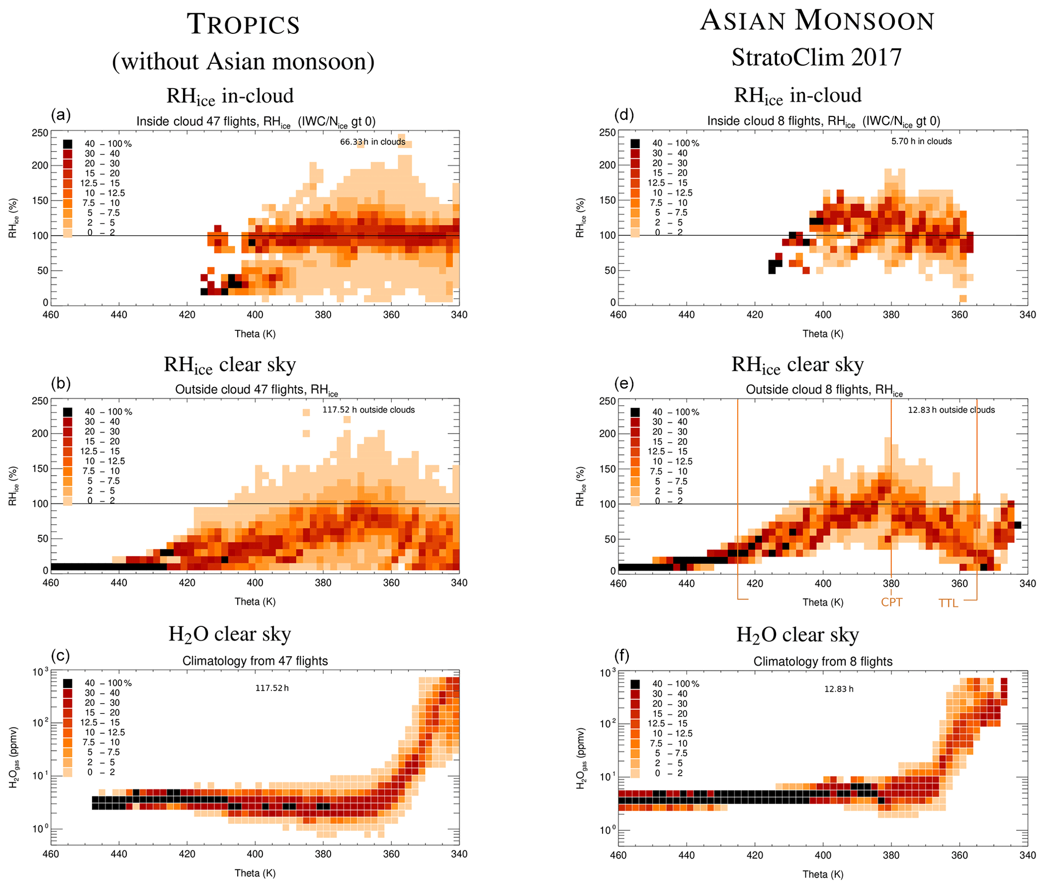
Figure 12 Climatology of humidity as a function of potential temperature Θ (left column, panels a–c: tropics without Asian monsoon; right column, panels d–f: Asian monsoon). The range of the TTL (after Fueglistaler et al., 2009) and the cold point temperature (CPT, derived from the observed temperature profiles) are marked in panels (b, e); the corresponding altitude range is ∼14 to 20 km. Note that in the tropics 355–330 ≈235–275 K (−38–0 ^∘C) and that the TTL spans from about 425 to 355 K. The field campaigns are listed in Table A2.

5.2.2 Potential temperature (Θ) parameter space

The high RH_ice values in and outside of cirrus clouds in the Asian monsoon are also visible in the Θ representation of the humidity (see Fig. 12d, e). In the tropical climatology outside of the Asian monsoon (Fig. 12a), RH_ice values most frequently center around saturation inside of the cirrus clouds. In the cloud-free TTL outside of the Asian monsoon (Fig. 12b), a humidification of the layer between ∼360 and 380 K to RH_ice around 90 % can be seen (for more details see Schoeberl et al., 2019).

In the Asian monsoon, on the other hand, the in-cloud RH_ice in the TTL exceeds saturation (Fig. 12d). In particular, between 380 and 400 K the most frequent RH_ice is around 130 %. Also outside of clouds (Fig. 12e), around the CPT supersaturation is frequently detected, and in general the humidification is higher than in the surrounding tropical regions. This is in agreement with Schoeberl et al. (2019), who reported high RH_ice coincident with the Himalaya monsoon during summer and closely associated with convection. The higher RH_ice in the Asian monsoon in comparison to the other tropical regions, influenced on the one hand by the stronger dynamics as mentioned in the previous section, can also be seen in the H₂O volume mixing ratios (Fig. 12c, f). In the tropics outside the Asian monsoon, the most frequent H₂O between 365 and 410 K is 1.5–4 ppmv, while in the Asian monsoon we found 3–8 ppmv, as also seen in the temperature parameter space. This finding is in accordance with other studies but has been observed in situ from aircraft directly in the Asian monsoon for the first time. For example, analyzing the air mass histories of higher in situ H₂O observations at other locations (highest values of 8 ppmv), Schiller et al. (2009) found that those air masses had passed the Asian monsoon region. Also, Ueyama et al. (2018) (and references therein) reported 5–7 ppmv at 100 hPa from Microwave Limb Sounder (MLS) observations and extensive model simulations over the Asian summer monsoon region.

5.3 H₂O and IWC for transport to the stratosphere

The H₂O transport to the stratosphere is regulated by the coldest temperature an air parcel experiences during transition through the tropopause region. The water amount passing the tropopause is set by the freeze-drying process associated with this transition (Jensen and Pfister, 2004) and is discussed to be as low as H₂O saturation at the minimum temperature (e.g., Schiller et al., 2009).

However, e.g., Rollins et al. (2016) showed for the ATTREX 2014 observations that the water vapor at the stratospheric entry point is higher by ∼10 %, because the water vapor depletion by ice crystals becomes increasingly inefficient at temperatures below 200 K (note that this is a rough estimate of the excess water vapor at the stratospheric entry point based on the actual temperature, which could be somewhat different from the minimum temperature of the air parcel's back trajectory). This is of importance, since already small amounts of H₂O can influence the stratospheric radiation budget (Solomon et al., 2010; Riese et al., 2012).

High supersaturations at the coldest points of the TTL are also discussed in Sect. 5.2.1. The ATTREX 2014 and also POSIDON 2016 observations are included in Fig. 9 (right column, panels d–f), where the most frequent in-cloud and clear-sky RH_ice at these temperatures can be seen to increase with decreasing temperature as discussed by Rollins et al. (2016). However, in the Asian monsoon measurements (Fig. 8, right column, panels d–f), RH_ice at the coldest temperatures is even higher above saturation than in the calmer tropics outside; the saturation is exceeded by about 20 %–50 % below 195 K. Therefore, we hypothesize that the conclusion of Rollins et al. (2016) might be extended: taking saturation at the stratospheric entry of an air mass as the set point for water vapor transport to the stratosphere, the transport is underestimated by ∼10 % in regions of weak convective activity. In convective regions the underestimation increased to 20 %–50 % in our observations. Note however that this hypothesize is based on a limited set of measurements and needs to be confirmed for the climatological conditions that prevail in the Asian monsoon TTL.

As mentioned earlier, the question of how much H₂O from convectively injected ice crystals is transported from above the CPT further into the lower stratosphere is a subject of recent research. In the study of Ueyama et al. (2018), it is concluded that over the Asian monsoon at 100 hPa, convection is the dominant driver of the localized H₂O and that nearly all of the convective enhancements in H₂O are due to the effect of convective humidification, while convectively detrained ice crystals have a negligible impact.

From our measurements in and above the Asian monsoon anticyclone, it is difficult to estimate to what extent cirrus cloud particles contribute to the amount of H₂O that might enter the stratosphere. Nevertheless, from Sect. 5.1 we know that the most frequent IWCs between about 365 and 400 K range from about 10 down to 0.5 ppmv. Above 400 K, up to 415 K some overshoots with IWCs between 0.5 and 8 ppmv are detected (Fig. 11d). These IWCs are similar to the amount of gas phase H₂O, which is between 3 and 8 ppmv in this region above the CPT (see last section). Such amounts of H₂O and IWC indicate that the air masses originate from an altitude of about 15 km (Fig. 3), which corresponds approximately to the lower boundary of the TTL (see Fig. 2).

The question remains of whether the ice particles found in the upper TTL will further grow and sediment out in supersaturated conditions (dehydration) or evaporate and add H₂O to the gas phase H₂O in subsaturation (hydration; see Jensen et al., 2007; Schoeberl et al., 2018). Inspecting the in-cloud RH_ice (see Fig. 12d) related to the respective IWCs, it can be seen that the air in the overshoots ≳ 400 K with the fairly high IWCs (0.5 to 8 ppmv) is subsaturated, while at lower altitudes both super- and subsaturation occur. This means that convective overshoots in the Asian monsoon can locally contribute a significant amount of water that might be further transported into the stratosphere. Unfortunately, we cannot say anything about the frequency of these events in this study.

Above the CPT in the surrounding tropics outside of the Asian monsoon, the in-cloud RH_ice values at ≳ 400 K are also subsaturated. Here, the IWCs range only between 0.02 and 2 ppmv, with some single data points up to about 2 ppmv. The related H₂O is 1.5 to 3 ppmv.

Comparing gas phase H₂O and IWC above the Asian monsoon CPT (both 3–8 ppmv) with the surrounding tropical regions (1.5–3 and 0.02–2 ppmv) might be an indication by in situ observations that, driven by overshooting convection, the Asian monsoon could be an important source for transport of H₂O to the stratosphere.

6 Global cirrus N_ice climatology from satellite remote sensing

Though the new in situ cirrus climatologies presented in Sect. 4 represent a considerable data set from research aircraft from which substantial insights are gained, it is still a mixture of different meteorological situations encountered during various field campaigns that does not necessarily display a statistically representative overall picture of the distribution of cirrus cloud properties. For this purpose, long-term global satellite remote sensing observations would be the method of choice, though retrievals of cirrus microphysical properties also have their own difficulties and limitations. This is especially true for the ice crystal number N_ice, which is particularly challenging to estimate from satellite remote sensing. The new retrieval method for N_ice introduced in Sect. 2.2, DARDAR-Nice, has however demonstrated the ability to satisfactorily reproduce in situ ice concentrations (Sourdeval et al., 2018a).

In this section, we show a global climatology of N_ice derived from DARDAR-Nice in the same presentation as the in situ N_ice climatology. Median N_ice, 25th and 75th, and 10th and 90th percentiles are provided for a global data set. In addition, median N_ice values are discussed for the Arctic region, the northern midlatitudes, the tropics, the southern midlatitudes, and Antarctica.

6.1 Comparison of remote sensing and in situ N_ice

As a base for reliable N_ice climatologies from satellite remote sensing, in situ measurements of PSDs (ice particle size distributions) from five campaigns of the Cirrus Guide II are used for an evaluation of the DARDAR-Nice retrieval algorithm (see Sect. 2.2). This directly follows the evaluation of DARDAR-Nice presented in Sourdeval et al. (2018a), in which a subset of campaigns from the Cirrus Guide II data set was used. This section therefore focuses on these five campaigns, which are nevertheless representative of a wide range of midlatitude and tropical ice clouds (see Fig. 1 and caption of Fig. 13). Figure 13a shows the N_ice frequencies of occurrence in 1 K temperature bins of the in situ measurements; the corresponding frequencies obtained from DARDAR-Nice are shown in panel (b). The latter are derived on the basis of two input parameters which are extracted from the in situ PSDs of the five campaigns listed in the figure caption, rather than being constrained from lidar–radar measurements during usual retrievals. This approach allows the identification of inherent incompatibilities between the satellite retrieval assumptions and the in situ measurements, by assuming that the in situ PSD parameters are perfectly constrained by the lidar–radar. Therefore, possible differences should only be attributed to other retrieval assumptions, such as the PSD shape. Sourdeval et al. (2018a) showed that this approach is efficient for identifying algorithmic limitations while still being representative of actual satellite retrievals. Note that DARDAR-Nice provides concentrations of ice crystals >5 µm, as it has not been evaluated for smaller sizes, while N_ice from in situ observations includes sizes >3 µm; however, the resulting difference in the ice concentrations is negligible. Also, the 1 Hz in situ PSDs are here sampled into 10 s averages to simulate the 1.7 km horizontal resolution of the DARDAR-Nice retrievals (assuming a flight speed of about 170 m s⁻¹).

Figure 13 N_ice–temperature climatologies from (a) in situ measurements during the field campaigns COALESC2011, ATTREX2014, ACRIDICON2014, ML-CIRRUS2014, and STRATOCLIM2017 and (b) satellite remote sensing, applying the algorithm DARDAR-Nice $f\left(N_{\mathrm{0}}^{\star },D_{\mathrm{m}}\right)$ to $N_{\mathrm{0}}^{\star }$. D_m derived from the in situ observations. The black contours represent the 25th, 50th, and 75th percentiles. Straight black line: DARDAR-Nice average median N_ice (0.064 cm⁻³); straight blue line: in situ average median N_ice (0.037 cm⁻³). The excess of N_ice by a factor of 1.73 in DARDAR is caused by the retrieval method; for more information see the text.

The black solid and dotted lines of the in situ climatology indicate the 50th, 25th, and 75th percentiles, which agree well with those of the entire in situ climatology (see Fig. 7b). This demonstrates that the selected subset is statistically representative of the entire database (indeed, the entire N_ice climatology contains only one additional campaign; see Table A2). A satisfactory agreement between DARDAR-Nice and the in situ observations is also seen, demonstrating that DARDAR-Nice N_ice retrievals match the in situ database for known size distributions very well.

A detailed comparison of the DARDAR-Nice percentiles (black solid and dashed lines) with those of the in situ observations, however, yields a small offset by a factor of 1.73, which is visualized in Fig. 13 by the average medians of DARDAR-Nice (straight black line, 0.064 cm⁻³) and in situ (straight blue line, 0.037 cm⁻³). One reason for this offset lies in the method of the retrieval. The two parameters, $N_{\mathrm{0}}^{\star }$ and D_m, calculated here from the in situ PSDs (usually from lidar–radar observations) are fed into a predefined four-parameter gamma-modified function to calculate ice particle size distributions (PSDs; see Sect. 2.2). N_ice is then calculated by summing up individual ice concentrations over a grid of size bins distributed over the gamma-shaped PSD for the entire range of observed ice crystal sizes (usually, a continuous integration of the PSD is performed). However, in the in situ measurements, there are often PSDs that do not contain ice particles < 20 µm; i.e., these size bins are empty. Such PSDs represent aged cirrus after the ice nucleation phase where the smaller ice crystals have grown to larger sizes (see Sect. 4.3.1). DARDAR-Nice, however, assumes a modified gamma distribution including all size bins, which partly explains the described positive offset. This behavior was also found by Wolf et al. (2019), who parameterized in situ-origin and liquid-origin cirrus from balloon-borne measurements by gamma functions. It is of note that when subtracting the ice concentrations of the “empty bins” of in situ PSDs from the retrieved DARDAR-Nice in a direct intercomparison, the agreement of N_ice is improved (not shown here). This is an important finding, as gamma functions are often used to represent cirrus PSDs, both in remote sensing retrieval algorithms and in global models. On the other hand it has to be noted that an offset on the order of a factor of 1.73 is tolerable given the variability of N_ice (6 orders of magnitude) and other possible error sources in the measurements, both in situ and remote sensing.

Other assumptions on the PSD shape by the satellite remote sensing method might also contribute to this bias. The PSD shape indeed is provided by four parameters, two of which are fixed and two are retrieved (see Sect. 2.2). Delanoë et al. (2014) showed that the two fixed PSD parameters defined by Delanoë et al. (2005) and used in DARDAR-Nice might lead to a too steep representation of the small ice mode (i.e., too high N_ice) and should be updated in future algorithm versions. Also, the bimodality of the PSD towards temperature where growth processes become important is not accounted for and usually leads to small positive N_ice biases (Sourdeval et al., 2018a). The causes of these assumptions are difficult to account for, as they most likely depend on the cloud type and on the thermodynamical environment, but they should to first order be reasonably captured by the 1.73 adjustment factor. Higher N_ice values in DARDAR-Nice towards low temperatures are also not surprising, as Sourdeval et al. (2018a) reported that the PSD parametrization used by DARDAR-Nice predicts higher concentrations of small particles (D_ice<25 µm) than the in situ comparative measurements. The overestimation increases with decreasing temperature, as the small ice particles dominate the PSDs more and more. This might be caused by a sharper representation of small ice concentrations in the PSD parametrization in comparison to the in situ small ice particle measurements below ∼210 K.

A further expected difference between the data sets arises from their detection limits. The lowest N_ice that can be detected by the in situ instruments is 10⁻⁴ cm⁻³; for the highest N_ice there is no limitation. Detection limits for DARDAR-Nice depend on lidar–radar sensitivity but are also influenced by the instrumental resolution, which may cause specific features to remain undetected. This effect, however, is represented in Fig. 13 by the 10 s sampling of 1 Hz in situ PSDs. Indeed, DARDAR-Nice misses the high N_ice in the temperature range 210–220 K, but these are young, line-shaped contrails which are too small scale to be detected by satellite. Also, part of the thinnest cirrus are not represented by DARDAR-Nice. This will be further discussed in the next section describing the global N_ice distribution from DARDAR-Nice.

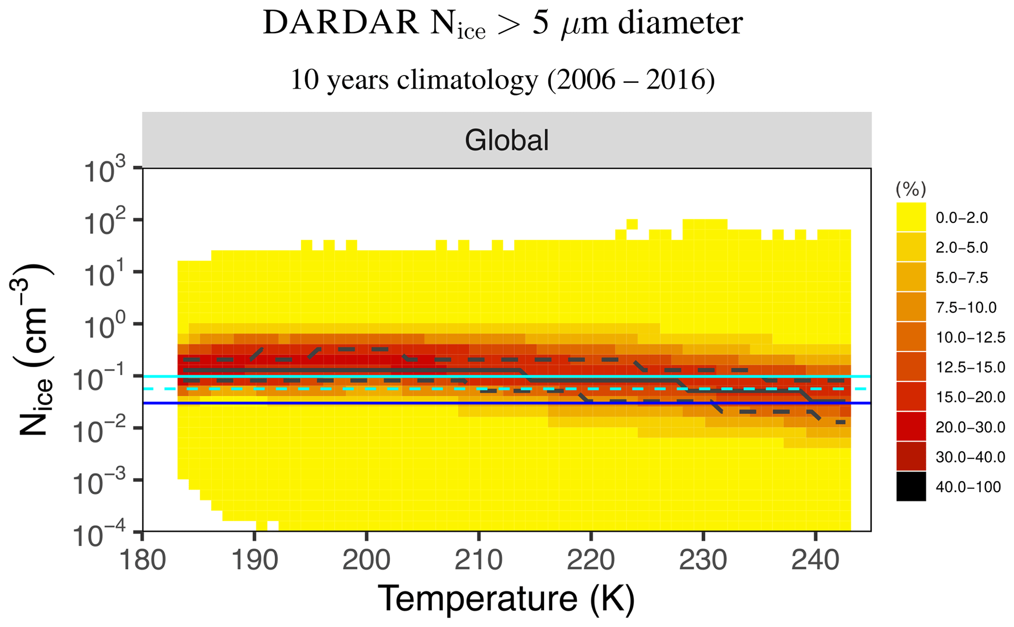
Figure 14 N_ice–temperature climatology from 10 years of satellite remote sensing observations using DARDAR-Nice. The data were collected twice a day, at midday and at midnight. Thick black lines: 25th, 50th, and 75th percentiles; thin plain cyan line: DARDAR-Nice median N_ice; thin dotted cyan line: DARDAR-Nice median N_ice adjusted to the offset factor of 1.73 between DARDAR-Nice and the in situ observations (see Fig. 13); blue line: in situ average median N_ice (from Fig. 7). Temperature intervals containing fewer than 10 retrievals were excluded (results not sensitive to exact threshold).

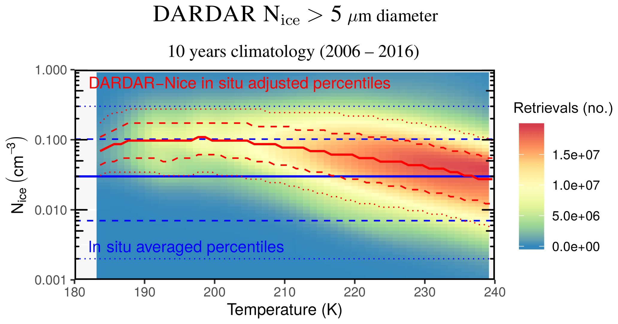
Figure 15 N_ice–temperature climatology across the entire N_ice–T parameter space. Red lines: global DARDAR-Nice percentiles (adjusted to the in situ observations by the offset factor of 1.73; see Fig. 13). The 10th and 90th, 25th and 75th, and 50th percentiles are indicated by dotted, dashed, and plain lines, respectively. Blue lines: in situ average percentiles (from Fig. 7). The percentiles are recommended for intercomparison with other data sets (the corresponding numbers are listed in Table 2); regional median N_ice values are shown in Table 3. The shaded background indicates the occurrence of retrievals, i.e., cirrus clouds. The cirrus appear most often at higher temperatures above about 225 K.

Overall, following the abovementioned arguments, an overestimation within a factor of 2 in DARDAR-Nice by comparison to the in situ data set is expected, although there is still some uncertainty as to how this overestimation will propagate globally and over various ice cloud regimes. The ratio of 1.73 in N_ice between DARDAR-Nice and the in situ data set, found from Fig. 13, should therefore be thought of as a minimum expected bias. Finally, the bias is expected to be stronger at low temperatures than at high temperatures, due to the increased likelihood of empty size bins as well as the higher importance of the representation of the small ice particle mode in the PSDs. A correction that depends on temperature, and possibly IWC, might therefore be optimal but a simpler first-order correction of 1.73 for all T and IWC ranges should here be sufficient for the needs of this study and considering the multitude of processes that can lead to this bias. Future studies will be required to precisely understand such inherent differences between satellite and in situ data set.

6.2 Global cirrus N_ice

The global frequency distribution of N_ice from 10 years of satellite observations is shown in Fig. 14. The data were collected twice a day, approximately at midday and at midnight (satellite Equator-crossing time is 01:30 and 13:30), from June 2006 to December 2016. It should still be noted that satellite retrievals are not continuously available throughout this period due to instrumental limitations, and nighttime retrievals are only available until 2011. This does not impact the conclusions presented here as diurnal cycles in N_ice are not considered in this study. Such variations are also difficult to quantify from lidar–radar products, although a diurnal signature has been investigated in the DARDAR-Nice N_ice data for tropical anvils (Wall et al., 2020). Overall, the global satellite data set consists of nearly 2×10¹⁰ N_ice retrievals. The color code represents frequencies of occurrence, and the black contours represent the 25th, 50th, and 75th percentiles.

From the median (solid black line), a slight increase in N_ice with decreasing temperature is visible, which is somewhat different to the in situ median N_ice (solid blue line, from Fig. 7b), where no temperature dependence is found. The DARDAR-Nice temperature dependence was already noted and discussed by Gryspeerdt et al. (2018). Another difference is that at T ≳ 210 K, the maximum N_ice of DARDAR-Nice reaches up to 100 cm⁻³, while the maximum in situ N_ice is only about 10 cm⁻³ (outside of young contrails).

The slightly increasing median N_ice with decreasing temperature might be attributed to homogeneous ice nucleation events, because homogeneous ice nucleation rates increase with decreasing temperature, but their appearance in space and time is transient, as discussed in Sect. 4.2.2. Such events are difficult to find by research aircraft and could be underrepresented in the aircraft observations.

The thinnest cirrus with low N_ice are represented by DARDAR-Nice for temperatures ≳ 190 K. At ≲ 190 K, however, a decreasing detectability of thin cirrus becomes apparent in the DARDAR-Nice climatology: in contrast to the in situ climatology, lesser or no thin cirrus are measured with decreasing temperature. The reason is that the colder the cirrus clouds, the smaller the ice crystals and the lesser their IWC (Fig. 10a, c). In the in situ N_ice climatology, in the TTL (≲ 205 K), an increased occurrence of very thin cirrus with N_ice around 0.001 cm⁻³ is reported in Sect. 4.3.1 and explained as aged cirrus consisting of only larger ice crystals. Though this type of clouds is partly missing in the DARDAR-Nice climatology, the median N_ice decreases again at these temperatures. This might reflect the frequent presence of aged thin cirrus. Note, however, that the statistics at these temperatures is based on a lower number of observations than at higher temperatures (see Fig. 15).

Table 2 DARDAR-Nice and in situ observation N_ice percentiles (as portrayed in Fig. 15) for intercomparison with global models or other data sets.

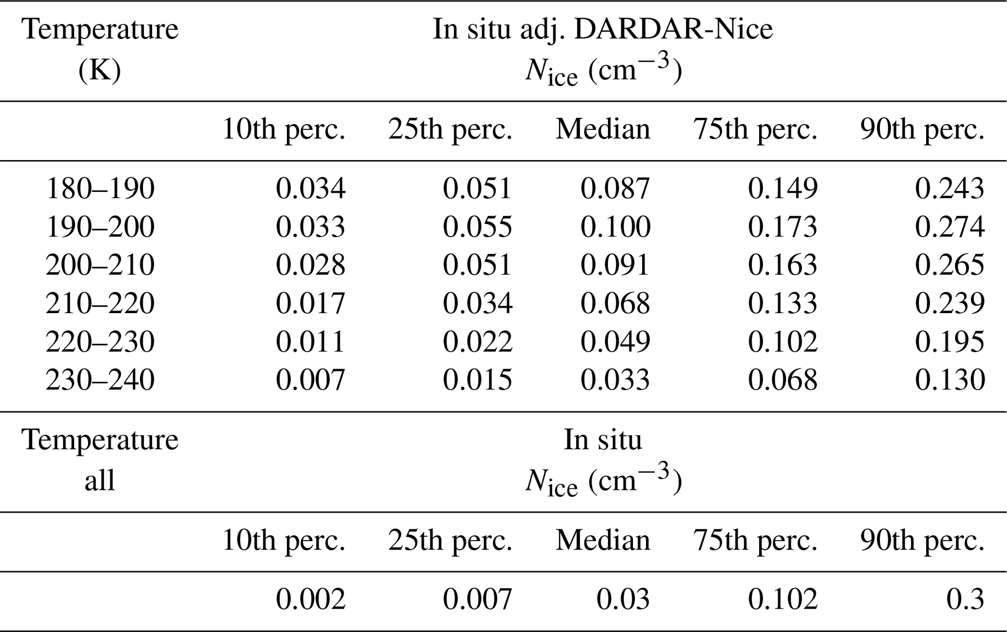
Table 3 DARDAR-Nice median N_ice (as portrayed in Fig. 15) for five regional latitude bands, Arctic: 90–67.7^∘, midlat. north: 67.7–23.3^∘, tropics: 23.3 to −23.3^∘, midlat. south: −23.3 to −67.7^∘, Antarctica: −67.7 to −90^∘, as well as global median N_ice. All temp.: median without temperature binning; T-int weighted: median using the relative occurrence of each temperature interval as a weight; most frequent: median considering those temperature intervals that contain 50 % of the total N_ice occurrence. T range denotes the respective minimum and maximum temperatures.

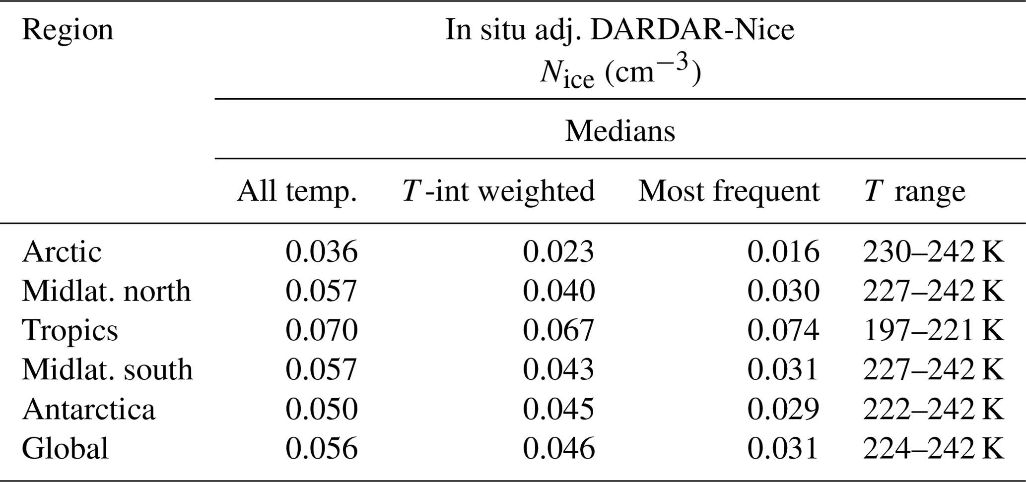
The median N_ice across all temperatures of the 10-year DARDAR-Nice climatology is about 0.100 cm⁻³ (Fig. 14, solid cyan line). Adjusting this number to the offset factor of 1.73 between DARDAR-Nice and the in situ observations reported in the previous section yields an in situ average median of 0.056 cm⁻³ (dashed cyan line; see also Table 3). It is nevertheless important to note that such a median is by construction computed assuming that all temperature bins have equal weight. When considering their actual relative occurrence as a function of temperature (see Fig. 15 and later discussion), the in situ adjusted global DARDAR-Nice median falls down to 0.046 cm⁻³. This is still larger than the average median of 0.03 cm⁻³ reported from the N_ice in situ climatology (blue line; from Fig. 7). Nevertheless, in light of the offset between the data sets, the decreasing detectability of thin cirrus by DARDAR-Nice, and other sources of error in both methods, the agreement between the DARDAR-Nice and the in situ N_ice climatology is good.

Altogether, both data sets have advantages and disadvantages: DARDAR-Nice has the advantage of the long, global time series where all atmospheric situations above the detection limit showing up at the times of observations are sampled. However, the thinnest cirrus at cold temperatures are not detected. Further, an offset is found between DARDAR-Nice and the in situ observations. On the other hand, the in situ N_ice climatology is based on a much smaller data set which is randomly distributed between different atmospheric situations. However, nearly the complete range of possible N_ice values can be detected by the in situ instruments.

For comparisons with other N_ice data sets or results from global models, the percentiles of the adjusted DARDAR-Nice and the average in situ N_ice values are shown in Fig. 14 and listed in Table 2 (note that an in situ data set slightly smaller than the data set presented here, but extended with regard to Krämer et al., 2009, is already used for this purpose by Bacer et al., 2018; Penner et al., 2018; Righi et al., 2020).

The DARDAR-Nice data set not only provides the N_ice distribution with temperature as shown in Fig. 14, but, as it also contains the entire spatial and temporal N_ice information, also the actual appearance of cirrus clouds in the N_ice–T parameter space. This is shown in Fig. 15, where the occurrences of DARDAR-Nice N_ice retrievals are indicated by the colored background. It can be noticed that, in regions of high frequency of occurrence (for T ≳ 210 K), the agreement between DARDAR-Nice and the in situ data set is best.

From this portrayal it can be seen that the cirrus clouds do not spread evenly across all temperatures, but that about 50 % of the cirrus appear at temperatures above about 225 K (see also Table 3, temperature range of global “most frequent” median N_ice). This clustering of cirrus at warmer temperatures, also reported by Yang et al. (2010) from CALIPSO cloud climatologies, is likely because in situ-origin and liquid-origin cirrus clouds are both found in this warmest and lowest cirrus layer, while at colder temperatures and higher altitudes only in situ-origin cirrus are present (see also Sect. 3.1 and Fig. 3). This vertical structure of the cloud types is also reported from observations by Krämer et al. (2016), Luebke et al. (2016), and Wolf et al. (2018); from global modeling by Gasparini and Lohmann (2016); from satellite and global modeling by Gasparini et al. (2018); and also from 12-year ERA-Interim data analysis in the North Atlantic region by Wernli et al. (2016).

Gasparini et al. (2018) provide global relative frequencies of liquid-origin cirrus with respect to temperature: more than 50 % of the cirrus clouds in the range between 235 and 220 K are of liquid origin, decreasing rapidly to about 20 % between 200 and 180 K. These findings from satellite observations and global modeling are reasonably consistent with those from trajectory analysis by Wernli et al. (2016), who reported the relative frequencies of liquid-origin cirrus with respect to pressure to decrease from about 55 % of the cirrus at 500 hPa (roughly 240 K) to 50 %, 30 %, and 5 % at 400, 300, and 200 hPa (roughly 230, 215, 200 K; see Fig. 2).

The analysis presented here provides the information that globally half of the cirrus are in the lowest, warmest cirrus layer between about 220 and 240 K, where, as mentioned above, about half of the cirrus are of liquid origin. This is of importance because of the differing radiative properties of in situ-origin and liquid-origin cirrus shown in Sect. 3.1.1 (see Fig. 5): if the thick liquid-origin cirrus clouds occur with such a high frequency, their strong cooling effect might exceed the much smaller warming effect of the in situ-origin cirrus, which could lead to a general cooling by cirrus.

Note that an analysis of N_ice in the IWC–T space, similarly to Fig. 6, is shown in Fig. 5 of the Supplement. This figure shows a good climatological agreement between the satellite product and the Cirrus Guide II data set, with very similar distribution of N_ice in the IWC–T space. Differences could be attributed to lack of statistics in Fig. 6 (noisy patterns). However, one notable difference is the slope of the IWC–T relation, which appears much flatter in the satellite product than in the in situ data, as indicated by the density isolines.

6.3 Regional cirrus N_ice

Lastly, we provide an impression of the regional variations in N_ice (see Table 3). To this end, subsets of the DARDAR-Nice data for five regional latitude bands between 90, 67.7, 23.3, −23.3, −67.7, and −90^∘ corresponding to the Arctic, midlat. north, the tropics, midlat. south, and Antarctica are considered, and three different N_ice medians are computed for each region and for the global data set. A first median (labeled “All temp.”) corresponds to the median N_ice value across all temperatures and considering all temperature bins to be equally probable, i.e., the same as used in Fig. 14. A second (labeled “T-int weighted”) represents the median using the relative occurrence of each temperature interval as a weight. The last (“Most frequent”) shows the most frequently appearing N_ice, considering those temperature intervals that contain 50 % of the total N_ice occurrence; T range denotes the respective minimum and maximum temperatures (note that in the in situ data set all three methods would yield to an identical median due to the flat temperature dependence).

Comparing the three median N_ice values, it is obvious that in most cases the “T-int weighted” and “most frequent” medians are smaller than those for “all temperatures”. This behavior is found because the cirrus clouds often appear at warmer temperatures (see previous subsection) where N_ice is moderate, which can be seen particularly in the most frequent medians, where the temperature range of the cirrus occurrence is given.

The global most frequent median N_ice is 0.031 cm⁻³ (in comparison to 0.056 and 0.046 cm⁻³ for all temperatures and T-int weighted) in the temperature range between 224 and 242 K (note that, to avoid representing mixed-phase clouds in the DARDAR-Nice analysis, 242 K is chosen as the maximum temperature). The lowest N_ice values are found in the Arctic (most frequent median 0.016 cm⁻³ between 230 and 242 K), which is most probably because the updrafts in the Arctic regions are generally lower than in other regions. In Antarctica, the most frequent median is higher (0.029 cm⁻³ between 224 and 242 K). This could be traced back to stronger orographic uplifts in austral winter. The boreal and austral midlatitude cirrus clouds are similar to the global, with most frequent medians of 0.030 and 0.031 cm⁻³ in the temperature range of 227–242 K. This points to moderate updrafts on average, though regionally orography and convection can cause higher updrafts and high N_ice, which is also shown by Sourdeval et al. (2018a).

Tropical cirrus clouds are different from those in the other regions. The most frequent cirrus have the highest median (0.074 cm⁻³) and appear at much colder temperatures (197–221 K), i.e., higher altitudes. This finding corresponds to the in situ observations presented in Sect. 3.1 (see Fig. 3) and also the DARDAR-Nice analyses of the vertical distribution of N_ice shown by Sourdeval et al. (2018a). The reason is the strong convection prevailing in tropical regions, lifting liquid-origin clouds up to high altitudes and cold temperatures, while also homogeneously nucleating a large number of in situ ice crystals (see also Sect. 5).

For all regions, except the tropics, more than half of the cirrus clouds are found at temperatures warmer than about 225 K and contain a considerable amount of liquid-origin cirrus, as discussed in the previous subsection. The same is true in the tropics, but for colder temperatures.

7 Summary and conclusions

The Cirrus Guide II aims to represent cirrus clouds and their environment from the perspective of in situ and satellite remote sensing observations. To this end, an in situ database is created, which is based on measurements with state-of-the-art instrumentation and extended in comparison to earlier studies (Schiller et al., 2008; Krämer et al., 2009; Luebke et al., 2013; Krämer et al., 2016). The in situ database consists now of about 168 h of ice water content IWC, 90 and 84 h of ice crystal number concentration and mass-mean radius N_ice and R_ice, 96 and 186 h of in-cloud and clear-sky RH_ice, and, correspondingly, 186 h of clear-sky water vapor (H₂O). The measurements span the altitude range between 5 and 20 km and cover the latitude band from 75^∘ north to 20^∘ south. The remote sensing database includes 10 years (2006–2016) of global ice crystal number concentration N_ice measurements. The main results from the evaluation of the two data sets are summarized in the following.

7.1 Characteristics and distribution of in situ-origin and liquid-origin cirrus (Sect. 3)

From the extended Cirrus Guide II in situ data set, we generally confirm the typical characteristics of in situ-origin and liquid-origin cirrus introduced by Krämer et al. (2016) with some additions (see Table 1).

• In situ-origin and liquid-origin cirrus consist of two subclasses determined by the updraft (1: slow updrafts – few large ice crystals form from heterogeneous freezing; 2: fast updrafts – many small ice crystals nucleate homogeneously).

  New in this concept is that liquid-origin cirrus also differ in the two updraft regimes. Often, the two subclasses occur in succession and form a bimodal size distribution.

• Liquid-origin cirrus are thicker (higher IWC) than in situ-origin cirrus and are usually characterized by larger ice crystals.

• The differences between the cirrus types are most pronounced in the formation phase of the clouds and are blurred with increasing lifetime due to ice crystal growth and sedimentation or additional ice formation.

In addition, we present a picture of the distribution of cirrus with respect to altitude and latitude, including an impression of the vertical structure of liquid-origin and in situ-origin cirrus (Fig. 3).

• Across all latitudes, the thicker liquid-origin cirrus predominate at lower altitudes, while at higher altitudes the thinner in situ-origin cirrus prevail. In between, the two cirrus types overlap. This finding is in agreement with Luebke et al. (2016) and Wernli et al. (2016) for midlatitude cirrus and Wolf et al. (2018) for Arctic cirrus.

Finally, a first estimate of the radiative characteristics of typical, specific, and idealized in situ-origin and liquid-origin cirrus scenarios is given (Fig. 5).

• Slow in situ-origin cirrus have a small optical depth (τ: 0.001–0.05), resulting in a slight net warming effect of not larger than about 1.5 W m⁻².

• The optical depth of fast in situ-origin cirrus is larger (τ: 0.05–1), but most of them are also warming (2–10 W m⁻²). The thickest fast in situ-origin cirrus at the lowest altitudes can change the sign of their net forcing; they switch to a slight cooling effect.

• Liquid-origin cirrus have large optical depths (τ: 1–12) and consequently exhibit a quite strong net cooling effect (−15 to −250 W m⁻²).

7.2 Cirrus and humidity in the tropical tropopause layer (TTL) (Sect. 5)

The new in situ data set is extended by observations in the tropical TTL outside, but also, for the first time, inside of the Asian monsoon anticyclone. Therefore, we put special emphasis on the analysis of the TTL environment.

TTL cirrus clouds (Fig. 11).

• Two types of most likely in situ-formed cirrus are identified in slow large-scale updrafts at low temperatures (T ≲ 205 K, Θ ≳ 355 K). The first is interpreted as young cirrus (N_ice around 0.1–1 cm⁻³ ≳ 3 µm diameter) and the second as aged cirrus (N_ice around 0.001 cm⁻³  ≳ 20 µm diameter) where the smaller ice crystals have grown to larger sizes.

• The highest N_ice (up to 30 cm⁻³ around the cold point tropopause, CPT) and IWC (up to 1000 ppmv around the CPT) are found in deep convective systems in the Asian monsoon. Such systems represent massive liquid-origin cirrus (very high IWC) superimposed by a fresh strong homogeneous in situ ice nucleation event (many small ice crystals ≲ 20 µm) in fast updrafts.

TTL humidity (Fig. 12).

• In the Asian monsoon, in-cloud and clear-sky RH_ice is higher (often supersaturated around and above the CPT) than in the surrounding tropics. This is caused by the stronger dynamics and a higher amount of H₂O in the Asian monsoon (most frequently 3 to 5 ppmv) in comparison to the tropics outside (1.5 to 3 ppmv).

• Taking saturation at the stratospheric entry of an air mass as set point for water vapor transport to the stratosphere, the transport is underestimated by ∼10 % in regions of weak convective activity (see also Rollins et al., 2016). In convective regions, the underestimation increased to 20 %–50 % in our observations in the Asian monsoon.

• Convectively injected ice over the Asian monsoon CPT (Θ ≳ 400 K, RH_ice≲100 %) can locally contribute a significant amount of water (up to an IWC of 8 ppmv, in comparison to only 2 ppmv in the surrounding tropics) that might be evaporated and further transported into the stratosphere.

7.3 In situ and satellite climatologies (Sects. 4 and 6)

Cirrus Guide II in situ cirrus and humidity climatologies.

• Median N_ice, R_ice, and RH_ice are presented in the IWC–T parameter space (Fig. 6).

  Distinct patterns are found: N_ice forms bands parallel to IWC, while R_ice is sorted diagonally in the IWC–T space. At tropical cold temperatures, supersaturations occur in thin as well as in thick cirrus.

• The entire extended data set (Fig. 7) is compared to the earlier studies (Fig. S6, Supplement).

  The median IWC and the core IWC band are the same in both data sets, showing that the in situ IWC measurement techniques are robust and that the IWC is a stable parameter describing cirrus clouds.

  The overall picture of the in-cloud and clear-sky RH_ice distributions has also not changed, demonstrating that high-altitude water vapor measurements that were under discussion earlier have improved and stabilized.

  An extended view is presented for N_ice, which is due to the better lower N_ice detection limit and a better mixture of the dynamical situation. The new N_ice–T percentiles are lower and show no distinct temperature dependence (average 10th, median, and 90th N_ice percentiles: 0.002, 0.03, and 0.3 cm⁻³) in comparison to the earlier observations that show a slight decrease in N_ice with temperature and an average median N_ice of about 0.1 cm⁻³.

• The in situ data set is subdivided into midlatitude and tropical climatologies (Figs. 8 and 9), and typical cirrus and humidity characteristics of the respective regions are presented.

DARDAR-Nice satellite global cirrus N_ice climatology

(Figs. 14 and 15).

• A global climatology of N_ice values from 10 years (2006–2016) of satellite observations is provided that can be used for comparison with global models or other data sets.

  The N_ice from satellite observations are validated by and adjusted to in situ measurements from a subset of five campaigns of the Cirrus Guide II.

• The global median N_ice from satellite observations is almost 2 times higher than the in situ median and increases slightly with decreasing temperature.

• N_ice medians sorted by geographical regions are highest in the tropics, followed by austral and boreal midlatitudes, Antarctica, and the Arctic.

• In the satellite climatologies of N_ice, half of the cirrus are located in the lowest, warmest cirrus layer and contain a significant amount of liquid-origin cirrus. Their global median N_ice is 0.031 cm⁻³.

• Regarding the frequent appearance of liquid-origin cirrus together with strong cooling effect is a motivation to investigate their influence on the overall cirrus radiative feedback on climate in future studies.

Appendix A: Methods

A1 Field campaigns and instrumentation

The field campaigns, locations, and deployed instruments are listed in Table A1, which is an extended version of the respective Table in the Cirrus Guide: Part 1. For a brief description of the instruments already introduced there, we refer to Krämer et al. (2016). Other instruments used during START 2008, CONTRAST 2014, ATTREX 2014, POSIDON 2016, and LTU 2012-2018 are briefly introduced here.

Table A1 Overview of campaigns and instruments. IWC: ice water content (uncertainties ∼20 %); RH_ice: relative humidity over ice (uncertainties ∼10 %–15 %); N_ice: ice crystal number concentration (uncertainties ∼10 %–100 %); the sampling rate of all aircraft instruments is 1 Hz.

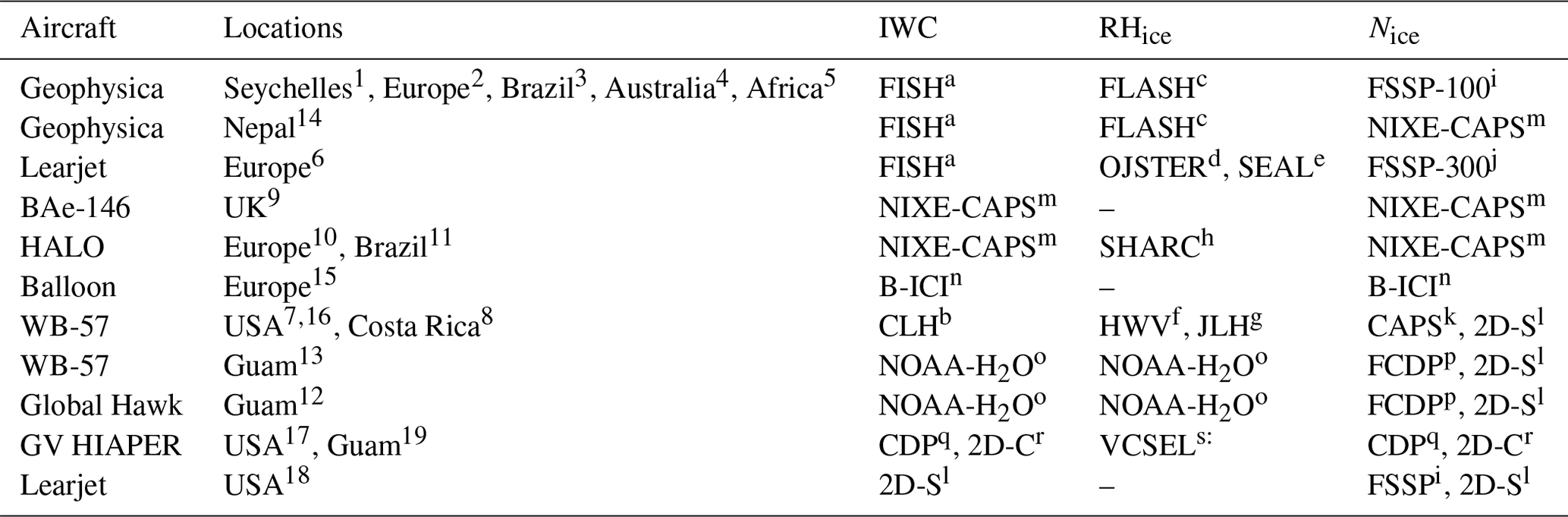
¹ APE-THESEO 1999. ² ENVISAT 2002, EUPLEX 2003, ENVISAT 2003. ³ TROCCINOX 2005. ⁴ SCOUT-O₃ 2005. ⁵ AMMA 2006. ⁶ CIRRUS 2003, CIRRUS 2004, CIRRUS 2006,, AIRTOSS-ICE 2013. ⁷ MidCix 2004, MACPEX 2011. ⁸ TC-4 2007. ⁹ COALESC 2011. ¹⁰ ML-CIRRUS 2014. ¹¹ ACRIDICON-CHUVA 2014. ¹² ATTREX 2014. ¹³ POSIDON 2016. ¹⁴ StratoClim 2017. ¹⁵ LTU 2012-2015. ¹⁶ CRYSTAL-FACE 2002. ¹⁷ START 2008. ¹⁸ SPARTICUS 2010. ¹⁹ CONTRAST 2014. ^a Lyman-α fluorescence hygrometer (Schiller et al., 2008; Krämer et al., 2009; Meyer et al., 2015). ^b Tunable diode laser hygrometer (Luebke et al., 2013). ^c Lyman-α fluorescence hygrometer (Sitnikov et al., 2007). ^d Tunable diode laser hygrometer (Krämer et al., 2009). ^e Tunable diode laser hygrometer (Buchholz et al., 2013). ^f Lyman-α fluorescence hygrometer (Rollins et al., 2014). ^g Tunable diode laser hygrometer (May, 1998). ^h Tunable diode laser hygrometer (Meyer et al., 2015). ⁱ Light-scattering cloud probe (Baumgardner et al., 2017). ^j Light-scattering cloud probe (Baumgardner et al., 2017). ^k Light-scattering and optical imaging cloud probe (Baumgardner et al., 2001). ^l Optical imaging cloud probe (Lawson et al., 2006). ^m Light-scattering and optical imaging cloud probe (Meyer, 2012; Luebke et al., 2016). ⁿ Cloud particle imager (Wolf et al., 2018). ^o Tunable diode laser hygrometer (Thornberry et al., 2017). ^p Light-scattering cloud probe (McFarquhar et al., 2007). ^q Light-scattering cloud probe (Baumgardner et al., 2017). ^r Optical imaging cloud probe (Baumgardner et al., 2017). ^s Tunable diode laser hygrometer (Zondlo et al., 2010). The campaigns under ^1–6 are described by Schiller et al. (2008), Krämer et al. (2009), and Finger et al. (2016), ^7–8 by Luebke et al. (2013) and Jensen et al. (2013b, 2009), ⁹ Jones et al. (2012), ¹⁰ Voigt et al. (2017), ¹¹ Wendisch et al. (2016), ¹² Jensen et al. (2017a), ¹³ https://espo.nasa.gov/posidon (last access: 29 September 2020), ¹⁴ http://www.stratoclim.org (last access: 15 January 2020), ¹⁵ Wolf et al. (2018), ¹⁶ https://espo.nasa.gov/crystalface (last access: 29 September 2020), ¹⁷ Pan et al. (2010), ¹⁸ Muhlbauer et al. (2014), and ¹⁹ Pan et al. (2017).

Table A2 Cirrus Guide II database for the IWC, N_ice, and RH_ice climatologies. y: quality-checked measurements; –: no or questionable measurements; an overview of each campaign is given in the Supplement; y^spe: N_ice is corrected for single-particle events (spe; see Sect. A2.2); y^⋆: N_ice from size-limited detection range (3–30 µm → contains ≳ 90 % of the ice particles), not spe corrected; y>15: N_ice from size-limited detection range (>15 µm → underestimating the full ice particle concentration), not included in the data analysis presented here; the campaigns written in italics are not contained in the occurrence frequencies. ^* S K L k: campaigns contained in the data sets of Schiller et al. (2008), Krämer et al. (2009), Luebke et al. (2013), and Krämer et al. (2016) (for S&K see Fig. S5 of the Supplement).

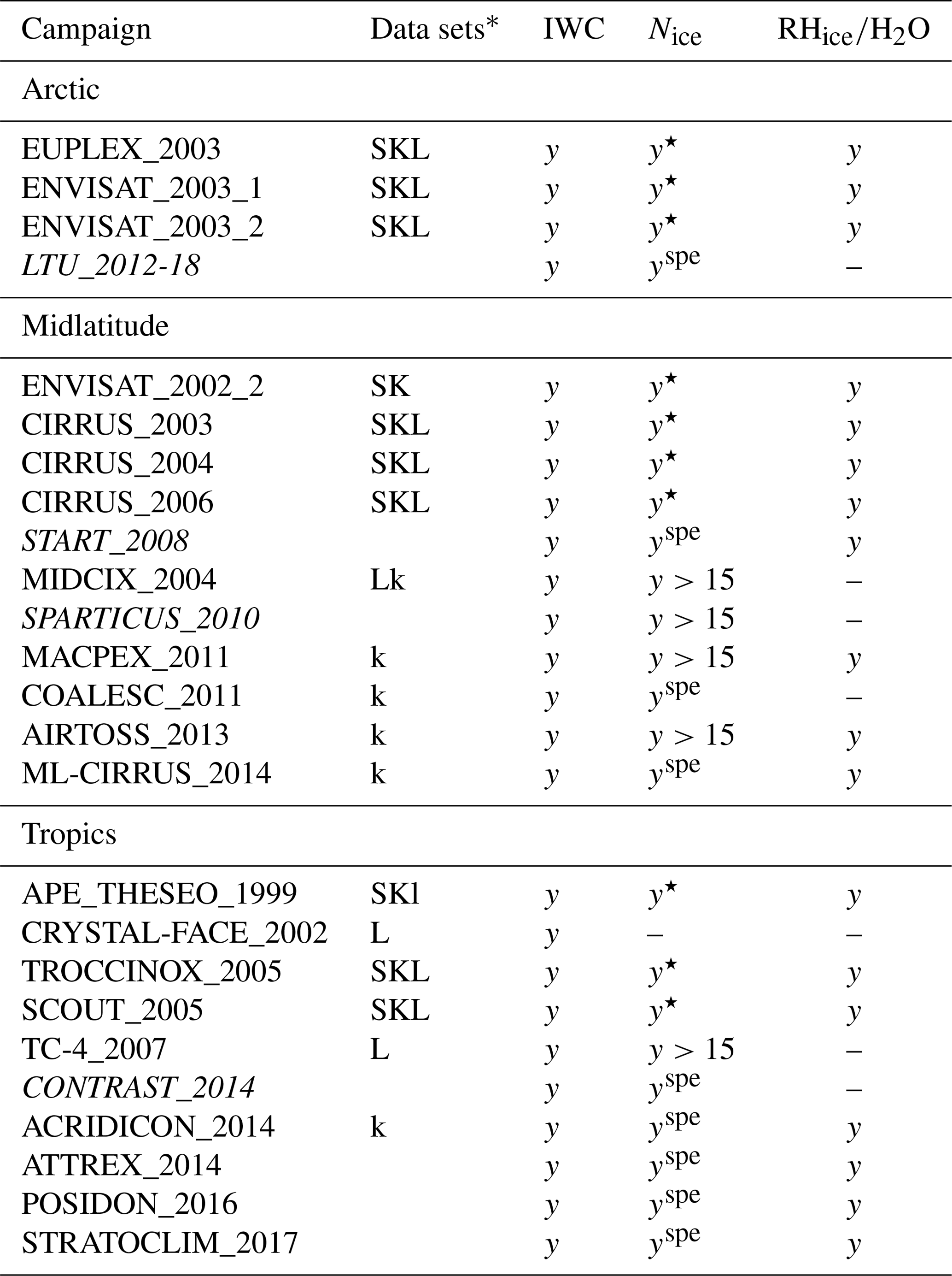
ATTREX 2014 and POSIDON 2016. IWC and RH_ice are measured with the dual-channel NOAA-H₂O instrument, a dual-channel TDL hygrometer which detects both ${{\mathrm{H}}_{\mathrm{2}}\mathrm{O}}_{\mathrm{tot}}$ ($={{\mathrm{H}}_{\mathrm{2}}\mathrm{O}}_{\mathrm{gas}}$ + IWC) and ${{\mathrm{H}}_{\mathrm{2}}\mathrm{O}}_{\mathrm{gas}}$ by using a forward- and a backward-directed inlet. The detection limit of the IWC is 0.03 ppmv (≈0.003 mg m⁻³). Cloud particle size distributions (PSDs) and thus N_ice are recorded by a FCDP and a 2D-S. The size range of the FCDP is 1–50 µm in diameter, and the 2D-S counts cloud particles between 25 and 3005 µm.

Start-08 and CONTRAST. IWC and N_ice are both derived from PSD measurements by a CDP and a 2D-C. The size range of the CDP is 2–50 µm in diameter, and the 2D-C counts cloud particles between 60 and 1100 µm.

LTU 2012–2018. IWC and N_ice are both derived from PSD measurements by the Balloon-borne Ice Cloud particle Imager (B-ICI), detecting ice particle sizes between 10 and 1200 µm in diameter. Note that the measurements are not from aircraft but from balloons launched at Kiruna, Sweden.

A2 Data evaluation methods

The data evaluation methods, detection ranges, and data quality criteria of the measurements of IWC, N_ice, R_ice, RH_ice, and H₂O are described in the following. The instruments measuring the respective parameters are listed in Table A1; the estimated uncertainties are mentioned in the table caption. For the calculation of frequency distributions of the data, only those campaigns where the measured parameters cover the same detection range are used, since mixing of data with differing detection ranges influences the calculation of percentiles. Thus, the list of analyzed campaigns varies for each parameter, since not all parameters are available for the same detection ranges in all campaigns, or the data quality is considered suspicious. In Table A2 the available parameters are listed for each campaign. The resulting data coverage of the parameters over the entire temperature range is shown in Fig. A1.

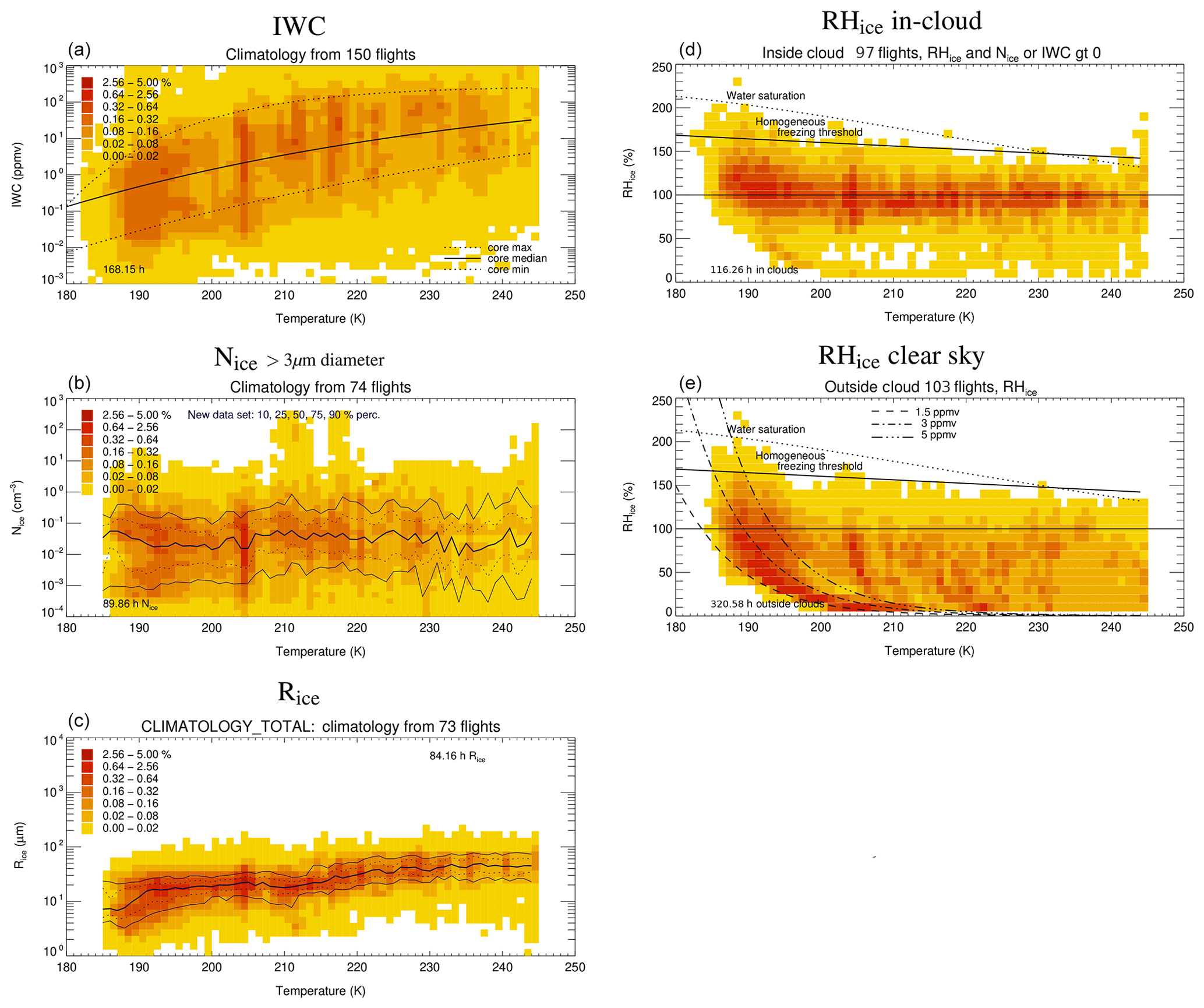
Figure A1 Data coverage of the Cirrus Guide II in situ database: IWC, N_ice, R_ice, and in-cloud and clear-sky RH_ice frequencies of occurrence as a function of temperature.

A2.1 Ice water content (IWC)

In the earlier studies of Schiller et al. (2008) and Luebke et al. (2013), the IWC was detected as the difference between total water (${{\mathrm{H}}_{\mathrm{2}}\mathrm{O}}_{\mathrm{tot}}$: water vapor + evaporated ice crystals) and gas phase water (${{\mathrm{H}}_{\mathrm{2}}\mathrm{O}}_{\mathrm{gas}}$); this product is named here IWC(H₂O). Krämer et al. (2016) also determined the IWC by integrating the ice particle size distributions (PSDs) measured by cloud spectrometers in cases where no total water measurements were available; we call this IWC(PSD). A detailed description of both methods is given in Afchine et al. (2018). Also, Afchine et al. (2018) demonstrated good agreement between the two methods under reliable sampling conditions. Agreement between IWC(H₂O) and IWC(PSD) is also a criterion for the quality of the IWC data (see also  Thornberry et al., 2017), as well as for the measurements of H₂O and the PSDs (for the data quality of H₂O and N_ice see also the following subsections).

Unlike in the earlier studies, we here combine the two methods, IWC(H₂O) and IWC(PSD). In case both measurements are available, IWC(H₂O) is used as the first choice for each flight second. But if IWC(H₂O) is zero or missing, IWC(PSD) is used. This combination of IWCs can fill times of measuring failures or signals beyond detection limits of one instrument and also compensates for some of the inhomogeneities in cirrus. If only one instrument is available, the respective IWC is taken.

As discussed by Schiller et al. (2008) and Afchine et al. (2018), the lower detection limit of IWC(H₂O) depends on the temperature and cannot be clearly defined. Data points below the lower dotted line drawn in the IWC–T parameter space in Fig. A1a represent observations where the difference between both the ${{\mathrm{H}}_{\mathrm{2}}\mathrm{O}}_{\mathrm{tot}}$ and ${{\mathrm{H}}_{\mathrm{2}}\mathrm{O}}_{\mathrm{gas}}$ measurements is not significant to unambiguously identify a cloud. This is where the ratio ${{\mathrm{H}}_{\mathrm{2}}\mathrm{O}}_{\mathrm{enh}}/{{\mathrm{H}}_{\mathrm{2}}\mathrm{O}}_{\mathrm{gas}}<\mathrm{1.07}$; note here that ${{\mathrm{H}}_{\mathrm{2}}\mathrm{O}}_{\mathrm{enh}}$ is the originally measured total water quantity, which is enhanced due to the sampling characteristics of the system (for more detail see Schiller et al., 2008; Afchine et al., 2018). The lower detection limit of IWC(PSD) is 0.05 ppmv (≈0.005 mg m⁻³) for NIXE-CAPS and 0.01 ppmv (≈0.001 mg m⁻³) for the combination of FCDP and 2D-C.

A2.2 Ice crystal number (N_ice)

From the campaigns where cloud particle size distributions (PSDs) are measured, we chose those where cloud particles between 3 and ∼1000 µm in diameter are recorded when calculating N_ice (see Table A2). We calculate N_ice as the sum of ice crystal concentrations over all size bins larger than 3 µm on a 1 Hz time resolution, because this time span represents around 200 m flight distance – which might already not resolve cirrus inhomogeneities. Thus, when averaging N_ice over longer flight times, cloud-free segments might influence the ice crystal concentrations.

Two instruments are needed to be deployed to cover the complete cirrus ice particle size range, one for smaller and the other for larger cloud particles. The PSDs from NIXE-CAPS (CAS-Depol + CIPgs) and FCDP + 2D-S are merged between 20 and 25 µm to avoid overlap of particle sizes, those of CDP + 2D-C at 55 µm. In earlier campaigns where only FSSP measurements (3–30 µm) are available, we calculate N_ice without the larger particles, since they contribute only a negligible part to N_ice (these campaigns are marked as y^⋆ in Table A2). However, for the calculation of occurrence frequencies only the campaigns covering the whole size range are used.

A2.3 Concentrations and frequencies of occurrence of small ice crystals: the effect of limited sampling volumes

N_ice is given by the number of cloud particle events recorded in the cloud volume that is sampled. Thus, the lowest concentration that can be detected is when only one particle is recorded. For the particle imaging probes (CIPgs, 2D-S, 2D-C, used size range ∼20–1000 µm) that results to $\sim {\mathrm{10}}^{-\mathrm{4}}$ cm⁻³, while for the light-scattering probes (CAS-Depol, FCDP, CDP, used size range ∼3–20 µm) it reaches the higher value of ∼0.015 cm⁻³. The difference in the recorded concentration range is caused by the differing sampling volumes of the two instrument types. As a consequence, N_ice concentrations ≲ 0.015 cm⁻³ contain only ice particles ≳ 20 µm. Lower concentrations of smaller particles cannot be detected with current particle measurement techniques (see also Krämer et al., 2016; Baumgardner et al., 2017).

Figure A2a exemplarily shows N_ice as a function of temperature, measured with NIXE-CAPS (NIXE-CAPS combines a CAS-Depol and a CIPgs) during the field campaign ML-Cirrus 2014, color coded by their frequencies of occurrence. CAS-DPOL samples 47.5 cm⁻³ at 190 m s⁻¹ aircraft cruising speed in 1 s while CIPgs probes about 1000–16 000 cm⁻³ as a function of particle size in the same time interval and aircraft speed (Costa et al., 2017). Thus, one particle event in the CAS-DPOL corresponds to a higher concentration than in the CIPgs. The red line in Fig. A2a represents the lowest detectable N_ice of CAS-DPOL and the blue line the same for CIPg. A notable feature in the figure is that directly above the lowest detectable N_ice of CAS-DPOL (red line) the N_ice frequencies jump to a higher level than below. The reason for this peak is an effect caused by the small sampling volumes of these instruments, which is often called “bad statistics”. It concerns instruments whose lowest N_ice detection limit is above the naturally occurring particle concentrations. When clouds with concentrations smaller than the lowest detectable N_ice are probed, these concentrations appear in the sampling volume as “single-particle events” (in the size range ≲ 20 µm) and are assigned to the minimum detectable concentration of the respective instrument, since the occurrence of one particle per time unit cannot be related to the true larger air volume it belongs to. Therefore, the data sets of this study are cleared from the artificial concentration feature at the instrument's detection limit by excluding N_ice caused by one single particle in the respective instruments.

The effect of this correction on the occurrence frequencies can be seen in Fig. A2b, which shows the same data set as panel (a), but with single-particle events removed: the sharp edge at the lowest detectable N_ice of the CAS-DPOL has disappeared; instead more lower concentrations from the CIPg become visible, which were hidden by the artificial concentrations from the CAS-DPOL single-particle events before.

Single-particle events are less common if the measurements are averaged over larger time periods. The considered time interval can be adapted according to the required spatial resolution of the measurements. However, as outlined above, for this study we choose to show the lowest time interval (1 s) to achieve the highest possible spatial resolution.

Figure A2 N_ice frequencies of occurrence for ML-Cirrus 2014: (a)  original data set, (b)  corrected for “single-particle events”. A further example of an uncorrected data set can be seen in Fig. S5 of the Supplement (middle left panel). For more details see text.

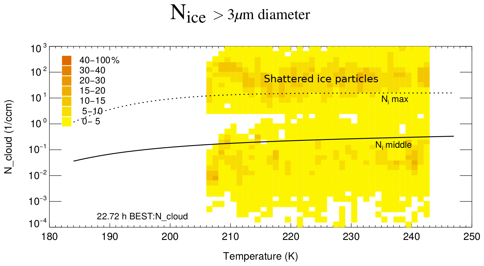
Figure A3 Example of N_ice measurements biased by shattering of large ice particles, visible in the frequencies of occurrence: high frequencies appear at N_ice concentrations between 10 and 100 cm⁻³ for all temperatures, which are not present in undisturbed measurements (see Fig. A2). The black lines denote the middle and maximum N_ice lines from Krämer et al. (2009).

Figure A4 Example of biased H₂O measurements, visible in the in-cloud RH_ice frequencies: inside of cirrus clouds, at temperatures ≳ 200 K, the frequencies should center around saturation (see Fig. 7d).

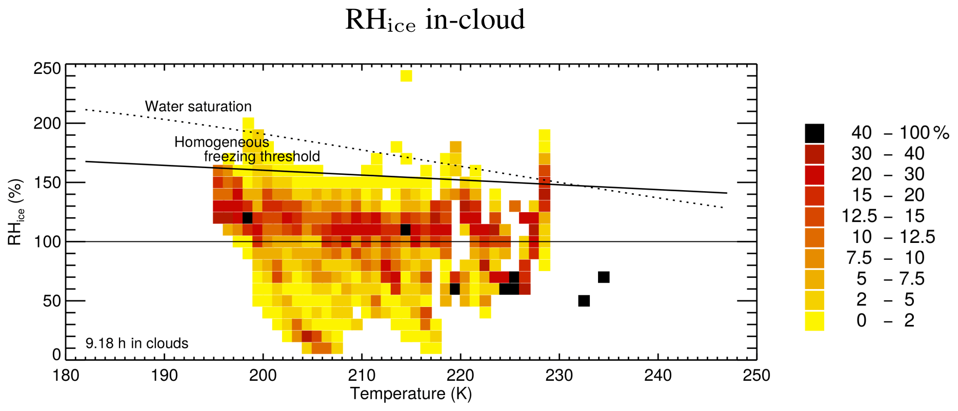
A2.4 Ice crystal shattering

Fragmentation of large ice crystals at the cloud probe housings distorted a correct recording of the ice crystal concentrations in earlier times. Today, new inlets and also postprocessing algorithms based on the interarrival times of the crystals in the sampling volume (Korolev and Field, 2015) have minimized this effect. Nevertheless, older data sets might be contaminated by small artifacts of shattered ice particles and need to be marked in the data set and not used in the data analyses. Shattering can be recognized when looking at the N_ice frequencies of occurrence plotted versus the temperature, as can be seen in Fig. A3, where an example of a data set including shattered ice crystals is shown. Clearly, high frequencies of occurrence appear at N_ice concentrations between 10 and 100 cm⁻³ for all temperatures. This ice particle “mode” is not present in data sets not influenced by shattered ice crystals, as can be seen when comparing Figs. A3 and  A2.

A2.5 Water vapor and relative humidity with respect to ice (H₂O and RH_ice)

Water vapor measurements where, as ice crystal concentrations, have been under discussion in the last decade (Peter et al., 2006). After some efforts to improve the quality of the measurements (e.g., Fahey et al., 2014), the water vapor instruments today provide high-precision data (see Rollins et al., 2014; Meyer et al., 2015; Thornberry et al., 2015; Buchholz et al., 2013; Kaufmann et al., 2018).

Nevertheless, we check the H₂O data quality for each campaign, including the recent ones, best-by comparison of several H₂O instruments as done by Kaufmann et al. (2018), for example. In case this is not possible, the frequencies of occurrence of in-cloud RH_ice are used to evaluate the quality of the measurements: inside of cirrus clouds, at temperatures ≳ 200 K, the frequencies should center around saturation, as can be seen in Fig. 7d. Figure A4 gives an example of a data set with a bias in the in-cloud RH_ice. We should note that such a distortion might also be caused by a shift in the temperature measurements, which we, however, have not yet observed. In any case, such data sets are not used for the data analysis.